| Issue |
A&A
Volume 620, December 2018
|
|
|---|---|---|
| Article Number | A98 | |
| Number of page(s) | 23 | |
| Section | Interstellar and circumstellar matter | |
| DOI | https://doi.org/10.1051/0004-6361/201832683 | |
| Published online | 05 December 2018 | |
Hot bubbles of planetary nebulae with hydrogen-deficient winds
II. Analytical approximations with application to BD + 30°3639
1
Leibniz-Institut für Astrophysik Potsdam,
An der Sternwarte 16,
14482 Potsdam,
Germany
e-mail: This email address is being protected from spambots. You need JavaScript enabled to view it.
; This email address is being protected from spambots. You need JavaScript enabled to view it.
2
Max-Planck-Institut für Sonnensystemforschung,
Justus-von-Liebig-Weg 3,
37077 Göttingen,
Germany
e-mail: This email address is being protected from spambots. You need JavaScript enabled to view it.
Received:
22
January
2018
Accepted:
13
September
2018
Abstract
Context. The first high-resolution X-ray spectroscopy of a planetary nebula, BD +30° 3639, opened the possibility to study plasma conditions and chemical compositions of X-ray emitting “hot” bubbles of planetary nebulae in much greater detail than before.
Aims. We investigate (i) how diagnostic line ratios are influenced by the bubble’s thermal structure and chemical profile, (ii) whether the chemical composition inside the bubble of BD +30° 3639 is consistent with the hydrogen-poor composition of the stellar photosphere and wind, and (iii) whether hydrogen-rich nebular matter has already been added to the bubble of BD +30° 3639 by evaporation.
Methods. We applied an analytical, one-dimensional (1D) model for wind-blown bubbles with temperature and density profiles based on self-similar solutions including thermal conduction. We also constructed heat-conduction bubbles with a chemical stratification. The X-ray emission was computed using the well-documented CHIANTI code. These bubble models are used to re-analyse the high-resolution X-ray spectrum from the hot bubble of BD +30° 3639.
Results. We found that our 1D heat-conducting bubble models reproduce the observed line ratios much better than plasmas with single electron temperatures. In particular, all the temperature- and abundance-sensitive line ratios are consistent with BD +30° 3639 X-ray observations for (i) an intervening column density of neutral hydrogen, NH = 0.20-0.10+0.05 × 1022cm−2, (ii) a characteristic bubble X-ray temperature of TX = 1.8 ± 0.1 MK together with (iii) a very high neon mass fraction of about 0.05, virtually as high as that of oxygen. For lower values of NH, we cannot exclude the possibility that the hot bubble of BD +30° 3639 contains a small amount of “evaporated” (or mixed) hydrogen-rich nebular matter. Given the possible range of NH, the fraction of evaporated hydrogen-rich matter cannot exceed 3% of the bubble mass.
Conclusions. The diffuse X-ray emission from BD +30° 3639 can be well explained by models of wind-blown bubbles with thermal conduction and a chemical composition equal to that of the hydrogen-poor and carbon-, oxygen-, and neon-rich stellar surface.
Key words: conduction / planetary nebulae: general / planetary nebulae: individual: BD + 30°3639 / stars: abundances / X-rays: stars
© ESO 2018
1 Introduction
In the late 1990s, space-based observations of the X-ray spectra from planetary nebulae became possible. Interpretation of nebular X-ray data from the XMM-Newton and Chandra telescopes then allowed essential new insights into the evolution, chemistry, and structure of planetary nebulae (Chu et al. 2001; Guerrero et al. 2001, 2002, 2012; Kastner et al. 2008; Yu et al. 2009; Nordon et al. 2009; Montez et al. 2010; Ruiz et al. 2011, 2013; Montez & Kastner 2013). Ongoing efforts today have culminated in the targeted Chandra Planetary Nebula Survey (ChanPlaNS, Kastner et al. 2012; Freeman et al. 2014; Montez et al. 2015).
ChanPlaNS is a volume-limited survey in which only planetary nebulae within a distance of ≃1.5 kpc were considered. Altogether, 59 objects could be compiled, either newly observed or retrieved (14) from the Chandra archival data. In general, X-rays have been detected as coming either from a point source at the position of the central star or as spatially extended (diffuse) emission emerging from the central “cavity” of the nebula, with detection rates of about 36% for point sources and about 27% for diffuse emissions (Freeman et al. 2014). A small number of objects have both kinds of emission. Typically, the diffuse X-ray emission occurs in nebulae with a nested shell morphology where the X-rays are confined by the inner rim. This diffuse emission is associated with rather compact nebulae with radii ≲0.15 pc only and occurs for about 60% of them (Freeman et al. 2014, Fig. 3 therein). It is still not clear whether this restriction of the diffuse X-ray emission to more compact objects is due to intrinsic wind properties as claimed by these authors, or to observational selection because the X-ray intensity may fall below the Chandra detection limit during the continued expansion of the bubble (see Fig. 6 in Ruiz et al. 2013 or Fig. 12 in Toalá & Arthur 2016a).
The question of possible differences between the detection rates of diffuse X-rays from nebulae with normal O-type or hydrogen-poor Wolf-Rayet ([WR] spectral type) central stars is interesting. According to Freeman et al. (2014), all four [WR]-type objects with rather compact nebulae observed so far with Chandra show diffuse X-ray emission, that is, a detection rate of 100%, which is in strong contrast with the lower detection rate of corresponding nebulae with O-type central stars.
An object of particular interest is BD + 30°3639 (BD + 30 for short, also known as “Campbell’s Star”; Campbell 1893). It was detected in X-rays by ROSAT (Kreysing et al. 1992) and turned out to be the brightest X-ray source of all planetary nebulae. Arnaud et al. (1996) analysed an X-ray spectrum taken with the ASCA satellite and found a prominent emission of Ne IX at 0.9 keV, suggesting a typical temperature of ~ 3 million K (MK) for the X-ray emitting plasma. Observations with the Advanced CCD Imaging Spectrometer (ACIS) aboard the Chandra space telescope (Kastner et al. 2000) showed a well-resolved X-ray emitting region and indicated that its “hot bubble” (HB) is asymmetric. The same observations led Kastner et al. (2000) to confirm the HB’s characteristic X-ray temperature of TX ≈ 3 MK. Using observations with the Suzaku satellite, Murashima et al. (2006) were able to estimate the ratios carbon-to-oyxgen (C/O) and neon-to-oxygen (Ne/O) which exceeded the solar ratios by factors of at least 30 and 5, respectively.In the context of a multi-wavelength study of BD +30, Freeman & Kastner (2016) also re-analysed the existing Chandra spectrum by means of a one-temperature thermal plasma model and came up with TX ≃ 2.6 MK for the X-ray emitting plasma.
Yu et al. (2009) were able to re-observe BD + 30 with Chandra to take the first X-ray gratings spectrum of a planetary nebula, using the Low Energy Transmission Gratings in combination with the Advanced CCD Imaging Spectrometer (LETG/ACIS-S). These high-resolution data allowed a detailed chemical and thermal characterisation of BD + 30’s HB. Based on a one-temperature plasma model, Yu et al. (2009) derived a characteristic X-ray temperature of 2.3 MK. An even better fit to the observation was achieved using a two-component plasma model in which the two components were found to have a temperature of TX = 1.7 and 2.9 MK, respectively. This finding implies that there exists a distinct temperature gradient in the HB of BD +30. For the element ratios C/O and Ne/O, Yu et al. (2009) found similar excesses as Murashima et al. (2006), namely, factors relative to solar of about 15–45 and 3.3–5.0, respectively.
In a similar fashion, Nordon et al. (2009) fitted a two- component plasma model to the Chandra spectrum of BD + 30 and found best-fit values of the X-ray temperatures of 1.9 and 3.0 MK, respectively. Beyond that, Nordon et al. (2009) used observations of BD + 30 with Chandra’s LETG Spectrometer to constrain the temperature jump at the contact discontinuity between the HB and the nebular rim. They concluded that the jump should be ≳ 930 000 K, thereby also constraining the efficiency of heat conduction and/or mixing of matter across the bubble-nebula interface (see below).
The investigations of Yu et al. (2009) and Nordon et al. (2009) support the expectation that the chemical composition of the bubble gas reflects the photospheric composition of BD + 30 which is extremely hydrogen-poor and rich in helium, carbon, and oxygen. The authors found very high C/O and Ne/O abundance ratios, which are not observed in the nebula but which are consistent with the stellar surface abundances found by Leuenhagen et al. (1996) and Marcolino et al. (2007).
The works of Yu et al. (2009) and Nordon et al. (2009) also suggest the presence of a significant radial temperature gradient across the bubble which, if confirmed, makes single-temperature approaches questionable. As shown by Steffen et al. (2008), heat conduction is an important physical process for the determinion of the bubble structure. Conduction naturally leads to a typical temperature distribution inside a HB with a very steep temperature gradient at the conduction front (i.e. the bubble–nebula interface), as energy is transported outwards from the hot, inner stellar wind to the much cooler nebular region.
Observational indications exist that suggest that stellar winds are inhomogeneous or “clumpy” (cf. Marcolino et al. 2007). Instead of (or in addition to) heat conduction, “mass-loading” by either hydrodynamic ablation or conductive evaporation of “clumps” can thus play a role. The analytical studies of Pittard et al. (2001a,b) show that the bubble density (temperature) will be increased (decreased) with respect to the adiabatic case. The detailed bubble structure depends critically, however, on the assumed boundary conditions (wind parameters and density profile of the environment) and the clump distribution. These studies did not include heat conduction, but we expect that it would dominate anyway because heat conduction changes the bubble structure “instantaneously” (Zhekov & Perinotto 1996).
Another possibility to reduce the temperature and to increase the density of X-ray emitting plasma is mixing of the bubble matter with cool nebular gas across the bubble–nebula interface (“contact discontinuity”) by Rayleigh-Taylor instabilities. The first “pilot” two-dimensional (2D) simulations of Stute & Sahai (2006), however, only cover a very limited time span (≲ 300 yr) and simple boundary conditions, and are thus not really suited for drawing conclusions concerning the temporal evolution of the mixing efficiency.
Much more realistic 2D simulations have been presented by Toalá & Arthur (2014, 2016a,b). They are based on post-AGB (post asymptotic giant branch) evolutionary tracks and realistic wind models in a similar manner to the simulations by Villaver et al. (2002) or Perinotto et al. (2004) and show clearly that mixing of bubble and nebularmatter across the bubble-nebula interface generates a region of gas with intermediate temperatures (approximatily mega-Kelvins) and densities, well suited to emit X-rays of the observed properties. The inclusion of heat conduction increases the amount of gas with these properties, and thus also the X-ray emission measure of the bubble, considerably.
A closer inspection of the Toalá & Arthur models shows, however, that they seem to overestimate the mixing process because the formation of a bright, sharply bounded nebular rim is obviously not possible (see Fig. 11 in Toalá & Arthur 2016b). This is clearly in contrast to the observationswhere nebular rims, once formed, persist over the whole nebular lifetime despite the obvious occurrence of instabilities. Moreover, one-dimensional (1D) simulations are quite successful in explaining the rim-shell morphology of planetary nebulae and their evolution with time (cf. Schönberner et al. 2014). We conclude that mixing, although it certainly does exist, cannot possibly generate sufficient amounts of gas to be responsible for the X-ray emission from planetary nebulae. Instead, it is mandatory to invoke heat conduction to explain the observations.
In general, thermal conduction changes the global structure of the bubble. Furthermore, the “evaporation” of nebular gas steadily increases the mass of the bubble during the evolution and soon dominates the bubble’s mass budget. If the bubble gas has a different chemical composition to the enclosing nebula, as is the case considered here, a chemical discontinuity will move from the conduction front inwards. If it is possible to detect, or to constrain, the position of a chemical discontinuity or the amount of evaporated matter, important insights as to the formation and evolution of [WR] central stars could be derived, apart from the proof that heat conduction is effective.
In Sandin et al. (2016, hereafter Paper I), detailed 1D rad- iation-hydrodynamics simulations of planetary-nebula models in which a stellar wind with a typical hydrogen-poor, [WR]-spectral type composition collides with a circumstellar envelope of hydrogen-rich composition were performed. These models describe the formation and evolution of hydrogen-poor bubbles inside normal nebulae, including heat conduction and the associated evaporation of hydrogen-rich gas into the bubble. It turns out that heat conduction (i) delays the formation of a bubble consisting of hydrogen-poor but carbon- and oxygen-rich matter considerably because of the high efficiency of radiation cooling around 0.1 MK (see Fig. 1 in Mellema & Lundqvist 2002), and (ii) does not lead necessarily to immediate evaporation (compare Figs. 5 and 6 with Fig. 7 in Paper I).
With all these still unsettled problems in mind, we considered it worthwhile to re-examine existing studies concerning the brightest X-ray source amongst planetary nebulae, BD +30. As the hydrodynamical model simulations are very time consuming, an extensive grid of model sequences with various choices of the relevant parameters is prohibitive. In the present paper, therefore, we present analytical, self-similar spherical models of hot bubbles with thermal conduction based on the formulations of Zhekov & Perinotto (1996, 1998, hereafter ZP96), but with various chemical compositions (hydrogen-rich, hydrogen-poor, and stratified), and examine their evolution. Questions to be addressed are the following:
-
Are one- (or two-)component temperature models sufficient for analysing the X-ray spectrum from a hot bubble whose structure is dominated by thermal conduction?
-
How is the X-ray spectrum and diagnostic line ratios, such as O VIII/O VII and Ne X/Ne IX, influenced by the bubble’s temperature profile and chemical composition?
-
Is the bubble abundance distribution consistent with the extremely hydrogen-poor and carbon-rich chemistry at the surface of the star?
-
Are there any indications that nebular hydrogen-rich matter evaporated into the hydrogen-poor bubble of BD +30 by heat conduction?
The paper is organised as follows. Section 2 explains the basic ingredients of our ZP96 bubbles controlled by thermal conduction: how they are constructed, how we compute their X-ray spectra, other relevant facts for interpreting the X-ray lines, and also the simplifications of our modelling. In Sect. 3, we discuss the differences of the analytical ZP96 bubbles to those computed by means of radiation-hydrodynamics simulations and show that analytical bubbles are able to reproduce the X-ray observations for BD +30. Section 4 is devoted to the analysis of the high-resolution X-ray line spectrum of BD+30 published in Yu et al. (2009) based on ZP96 bubbles with homogeneous hydrogen-deficient WR chemical composition. In Sect. 5, we introduce bubbles with inhomogeneous chemical composition and address the question whether the hot bubble of BD +30 may already contain a small amount of evaporated hydrogen-rich nebular matter. After the discussion (Sect. 6), the paper closes in Sect. 7 with a summary and conclusions.
Preliminary results of this work have been presented at IAU Symposium No. 323 (Schönberner et al. 2017).
2 Methods
2.1 Temperature and density structure of a bubble
The equations of ZP96 are based on the work of Weaver et al. (1977) on bubbles formed by spherically interacting winds that include heatconduction but also take into account the wind evolution of the central star. They provide us with the temperature and ion density structures as a function of time and bubble radius. Most importantly, this analytical, self-similar model is much faster to implement numerically than a full hydrodynamical code. It is assumed (i) that the HB is hot enough (≳ 106 K) to be isobaric, (ii) that the optical nebula (more precisely the nebular rim) is very thin compared to the extension of the HB (ZP96 call this the “thin-shell approximation” 1), and (iii) that the rim expands much faster than the outer slow wind. We add that the ZP96 models explicitly account for the mass accretion through the outer boundary (conduction front) due to the evaporation of ambient (rim) matter.
The efficiency of heat conduction is characterised by the conduction constant C, which ranges between 3 × 10⁻⁷ erg cm−1 s−1 K−7∕2 for a hydrogen-free WR composition (see next section) and 6 × 10⁻⁷ erg cm−1 s−1 K−7∕2 for a bubble consisting of hydrogen-rich matter. The equations of ZP96 can only be solved for constant C, whereas in realistic bubbles with a chemical gradient, C depends on the radial distance to the central object, r. Hence, we also used an intermediate value of 4.5 × 10⁻⁷ erg cm−1 s−1 K−7∕2 applicable for bubbles with a stratified composition, that is, for those where the outer bubble layers consist of H-rich instead of WR matter. For the dependence of the heat transfer efficiency C on effective ion charge Z, or plasma abundance, further details can be found in Sandin et al. (2012) and Paper I. In this context we want to remark that Christer Sandin (priv. comm.) pointed out that very often a conduction constant C is used in the literature that is a factor oftwo too high2.
A rangeof boundary conditions and input parameters is required to solve for the HB temperature and density structures. These constraints are given by the velocity of the fast wind from the central star, vfw (t), the mass-loss rate mediated by this wind, Ṁfw(t), the constant velocity of the slow outer wind, vsw, and the constant mass-loss rate of the outer wind, Ṁsw (see ZP96 for details). We numerically solve their differential equation (Eq. (9) in ZP96) for the dimensionless temperature ξ, starting from ξ ≈ 1 (at the outer boundary of the HB). Together with Eq. (5) in ZP96 for the position of the reverse wind shock, the full structure of the bubble follows after conversion of the dimensionless similarity solution into real physical units.
Constancy of Ṁsw and vsw means that the ambient density immediately ahead of the rim falls off with distance as r−2 . Hydrodynamical models show that the shell is a rarefaction wave such that the flow velocity at its inner edge (i.e. ahead of the rim) only changes by tens of km s−1 during the whole evolution while the stellar wind luminosity varies by orders of magnitude at the same time. Thus, we feel that the assumption of constant slow-wind parameters is an acceptable compromise.
The range of the mass-loss rate and flow velocity of the slow wind that we used as outer boundary conditions for the bubble evolution is given in Table 1. Together with three choices of the conduction parameter and the chosen ages, a total of 945 parameter combinations follows. The actual number of models, however, is lower because of parameter degeneracy due to the fact that the bubbles’ inner and outer radii (and their temperature and density distributions as well) are functions of Ṁ sw ∕vsw (Eqs. (10)–(12) in ZP96).
Hanami & Sakashita (1987) also found self-similar solutions for wind-blown bubbles with heat conduction. The difference with the ZP96 models used here are the boundary conditions: Hanami & Sakashita employed variable outer boundary conditions but kept the inner, that is the stellar wind paramters, fixed. This approach is applicable to the case of massive O-type stars whose winds remain virtually constant over the expansion time of the bubble and cannot be used here where the stellar parameters, including the stellar wind, change on timescales that are comparable to or even shorter than the expansion time of the wind-blown bubble.
Parameter grid of our bubble simulations.
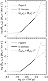 |
Fig. 1 Variations of the quantities |

2.2 Parametrisation of the system
ZP96 used the 0.605 M⊙ central-star model sequence of Blöcker (1995) to parametrise the time dependence of the stellar wind parameters. Here we want to model bubbles with hydrogen-deficient and helium- and carbon-enriched compositions as they are expected for planetaries around nuclei with [WR] spectral-type characteristics. As evolutionary calculations are not yet available, we must resort to empirical relations for central-star and wind evolution. Therefore, we used recent results of spectral analyses of a large sample of [WR] central stars (see e.g. Todt & Hamann 2015), which are compiled in Table 4 and visualised in Fig. 4 of Paper I. This figure shows that (i) the wind luminosity of [WR] central stars increases much faster with effective temperature than is predicted by Pauldrach et al. (1988) for the case of normal, hydrogen-rich central stars while (ii) the wind speed is considerably lower. For instance, at the stellar temperature of BD +30, ≃ 50 000 K, [WR] central stars have mass-loss rates higher by about two orders of magnitude, that is, of about 10−6 M⊙ yr−1 (instead of 10−8 M⊙ yr−1) while the wind speed is only about 800 km s−1 (instead of 1700 km s−1). Altogether, the important wind luminosity is about 10–20 times the typical value expected for hydrogen-rich central stars (cf. Fig. 4 in Paper I).
Instead of the 0.605 M⊙ post-AGB evolutionary track, here we employed the 0.595 M⊙ track introduced by Schönberner et al. (2005, see Fig. 1 therein). Of course, the evolutionary speed of this model across the Hertzsprung–Russell diagram (HRD) is based on hydrogen burning together with the Pauldrach et al. (1988) mass-loss prescription, both of which are surely inadequate for a description of AGB remnants with a hydrogen-poor or -free stellar surface. In order to comply with the expected faster evolution of an AGB remnant that burns helium and emits a comparatively more powerful wind, we accelerated the evolution of our 0.595 M⊙ model by a factor of 5.5. This acceleration ensures that the post-AGB age of the model is 730 yr at Teff = 50 000 K, close enough to the estimated kinematical age3 of BD +30 of 800 yr (Li et al. 2002). This new evolutionary track is then considered to be an approximate representative for the evolution of the central star of BD +30.
We proceeded to link the mass-loss model as presented by the thin lines in Fig. 4 of Paper I to the stellar parameters of our new 0.595 M⊙ post-AGB model sequence. For simplicity, this mass-loss model is an appropriately scaled Pauldrach et al. (1988) model that reproduces the observed mass-loss parameters of BD +30 quite well and is characterised by Ṁfw and vfw. ZP96 introduced the quantities  and Ṁfwvfw whose time evolution is presented in Fig. 1 in terms of the dimensionless parameter τ = t∕103 yr for the case studied in this paper.
Figure 1 demonstrates clearly that during the most important part of the modelled evolution, between about 160 and 800 yr, both quantities can be well approximated by the power laws indicated in the figure. These fits fix the parameters β1 = 6.19, β2 = 4.4 (β = β1∕3 + 1 = 3.06 for βp = −2), which are necessary for solving Eq. (9) of ZP96. The position of the reverse wind shock, the inner boundary of the bubble, is then also fixed by Eq. (5) of ZP96. Moreover, 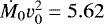 M⊙ yr−1 (km s−1)2 and Ṁ0v0 = 3.07 × 10⁻³ M⊙ yr−1 km s−1. Having the wind evolution fixed, the only free parameters left are then (i) the age of the bubble, (ii) density and velocity of the ambient matter (= nebular shell), given by the constant values of Ṁ sw and vsw , and (iii) the coefficient of thermal conduction, C, necessary for solving the dimensionless temperature equation of ZP96.
Once the radial runs of temperature and density are solved for the selected C, the density is split into ion and electron densities according to the two abundance distributions (either “WR” or “PN”, depending on C) listed in Table 2. Complete ionisation is assumed, which is not quite correct (see e.g. Fig. 3) but is a reasonable approximation for our purpose.
The WR element distribution closely corresponds for the main elements He, C, and O to the photospheric composition of BD +30 after Marcolino et al. (2007), while the PN element mixture is typical for Galactic-disk planetary nebulae. Leuenhagen et al. (1996) arrived at nearly the same abundances for BD +30 as Marcolino et al. (2007). We note, however, that Crowther et al. (2006) report a smaller C/O ratio of about five instead of 12 as used here, and a correspondingly higher helium fraction. The photospheric hydrogen content of BD +30, if there is any, is uncertain, and we assume here a mass fraction of 2%, that is, a reduction by a factor of 34. Except for the assumed small hydrogen content, the WR elemental mixture used here is typical for the intershell region of AGB stars, exposed by some still unknown evolutionary process4 .
Since we had to compute complete X-ray spectra with all existing lines included, all those elements that are not easily accessible to observationswere supplemented, assuming solar mass fractions (see Table 2). Due to the high oxygen content of the WR mixture, all these elements have abundances relative to oxygen of about one tenth solar (by number). Exceptions exist for nitrogen and neon. Complete CNO hydrogen burning converts virtually all C and O nuclei into nitrogen, which is later “burned” into neon (22 Ne) within the pulse-driven, convective helium-burning shell; that is, there is a one-to-one correspondence between the CNO ashes (14 N) and the neon produced during a thermal pulse. Depending on the efficiency of the third dredge-up, very high neon abundances may be produced within the intershell region. The neon of the WR mixture is thus essentially 22 Ne, in contrast to the PN mixture where 20Ne is the dominant isotope.
From the CNO abundances of the PN mixture (cf. Table 2, Col. 6), we derived an intershell neon abundance of 0.022 (by mass) for the stellar photosphere and wind, which we then adopted for our WR composition. The nitrogen abundance was set virtually to zero (mass fraction of 10−5). We note in this context that Marcolino et al. (2007) estimated a neon mass fraction of ~ 2 %, consistent with the value used here (Table 2).
The photospheric nitrogen content of BD +30 is not known. For a number of late-type [WR] central stars, however, nitrogen abundances of up to a few percent (by mass) have been found (cf. review of Todt & Hamann 2015). Such high amounts of nitrogen are a signature of simultaneous non-equilibrium burning and mixing of hydrogen at the interface between the envelope and the stellar core as occurs if a thermal pulse happens when the central star evolves across the HRD towards the white-dwarf stage (“late” or “very-late thermal pulse”). Ourchoice of a virtually zero nitrogen abundance implies complete hydrogen burning without mixing and complete loss of all unburned hydrogen such that the nitrogen-free, but neon-rich, inter-shell layers become exposed.
Figure 2 (left) illustrates the physical structure of a typical, middle-aged HB, computed with the same parameters but different heat conduction constants C according tothe two abundance sets used. We see temperature distributions typical for heat conduction, with a very steep gradient at the conduction front at 1.54 × 1016 cm distance from the star (located at the origin). The bubble with the hydrogen-deficient composition is hotter with a somewhat steeper temperature gradient because of the smaller heat conduction efficiency. The pressure in both bubbles is the same because of the identical boundary conditions, hence the particle densities (ions plus electrons) must be different.
We repeat that the parameters for the slow wind, Ṁsw and vsw, into which the bubble and its swept-up shell (i.e. the nebular rim) with the forward shock expand are assumed to remain constant throughout the whole bubble evolution. In reality, the bubble and its swept-up shell (rim) is expanding into an expanding shell that has earlier been set up by photoionisation driven by the hot central star. Density and velocity immediately ahead of the forward shock are expected to change with time, that is, Ṁ sw and vsw do not remain constant. Also, their present values are not known, unless a full radiation-hydrodynamics model fitted to BD +30 becomes available. We therefore adopted quite large ranges for Ṁ sw and vsw (cf. Cols. 3 and 4 in Table 1) in order to cover all possible values of these parameters.
From the physical point of view, the bubble’s mass increases by stellar wind matter passing through the reverse shock and by “evaporation” of nebular matter through the heat conduction front, where the latter contribution to the bubble’s mass budget even dominates in the later stages of evolution (Steffen et al. 2008, Figs. 6 and 8 therein). However, the chemical composition within the bubble is implicitly assumed to remain the same over time. This is of no concern for models containing normal matter since wind and evaporated gas from the nebula have the same composition. Our bubble models with WR composition are therefore physically inconsistent. The evaporated matter is normal, hydrogen-rich PN matter, and since the latter is more important for the bubble’s mass budget, a composition “discontinuity” will develop inside the bubble and will move slowly inwards with time. The actual position of this chemical discontinuity depends on the relative sizes of the wind’s mass input and the evaporated mass driven by thermal conduction and how both develop with time.
In the context of these considerations, the construction and time evolution of ZP96 bubbles with a homogeneous hydrogen-poor chemical composition implicitly means that the evaporated matter has the same hydrogen-poor composition as well, which, of course, is unrealistic. Nevertheless, we study the properties of such models with homogeneous WR composition for two reasons: (i) the qualitative dependence of the bubble properties on the boundary conditions is independent of the assumed chemical composition; (ii) they are the basis for bubbles with inhomogeneous composition, that is, bubble models with additional amounts of hydrogen-rich matter. The construction and use of chemically inhomogeneous bubbles is, however, postponed to Sect. 5.
Despite the limitations necessary to derive analytical similarity solutions for heat-conducting wind-blown bubbles, they turned out to be a very useful tool for investigating the physical properties of these bubbles and analysing their X-ray emission in terms of temperature and chemical composition, as we demonstrate in Sect. 4.
Chemical compositions of the stellar photosphere and wind (WR) and the nebular gas (PN) used in this work, arranged by order of atomic number Z as mass fractions (Cols. 3 and 5) and (logarithmic) number fractions (ϵ) relative to hydrogen (Cols. 4 and 6).
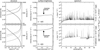 |
Fig. 2 Examples of bubble structures (left panels) and X-ray emissions (middle and right panels) for hydrogen-rich (PN, top panels) and hydrogen-poor (WR, bottom panels) composition. The inner boundaries are at the position of the reverse wind shock (0.67 × 1016 cm), the outer boundaries at the (heat) conduction front at 1.54 × 1016 cm. The planetary nebula proper is on the right side of this front. Both HBs have a similar parameterisation: age = 500 yr, Ṁ sw = 10−5 M⊙ yr−1, vsw = 25 km s−1 , but C = 6 × 10⁻⁷(top panels) and C = 3 × 10⁻⁷ erg cm−1 s−1 K−7∕2 (bottom panels). The bubble structures are characterised by the radial runs of electron temperature (solid), total particle number density (long dashed), ion number density (dashed), and electron density (dotted). We note the linear scale for the temperature, but the logarithmic scale for the densities. The characteristic X-ray temperatures of the bubbles are 2.9 MK (PN) and 2.4 MK (WR), respectively. The intrinsic X-ray surface brightnesses of these two bubble models are displayed in the middle panels and correspond to the emission (spectral luminosity density) in wavelength bands of 5–40 Å (0.3– 2.5 keV) shown in the right panels. The positions of the respective wind reverse shocks (= inner bubble boundaries) are indicated by the arrows. The X-ray luminosities in the given wavelength band are 3.7 × 1032 erg s−1 (PN) and 1.5 × 1034 erg s−1 (WR). |
2.3 Computation of X-ray spectra with CHIANTI
We used CHIANTI software package (v6.0.1, Dere et al. 1997, 2009) to compute the X-ray emission spectra of our ZP96 bubbles. One of the key distinctions between our analysis and earlier assumptions of isothermal plasma components lies in the capability of the ZP96 theory to model the temperature variation over the HB radius. Different gas temperatures translate into different HB regions, where a given chemical element will show different stages of ionisation (see Fig. ??). These ionisation fractions are independent of the electron density5 .
We first computed the maximum temperature at the inner boundary of a HB (the position of the reverse shock) and located then the outer radius at which the temperature has decreased to 105 K. In young, relatively cool HBs, our procedure typically results in about 30 radial steps and an equal amount of sub-spectra. For evolved HBs with maximum temperatures of several mega-Kelvin, the steep temperature decrease towards the outer regions yields up to several hundred sub-spectra. These sub-spectra were then merged into an integrated, pseudo-observed spectrum but neglecting all the observational complications such as extinction and instrumental properties. We restricted ourselves to the spectral window between 5 and 40 Å, according to the Chandra observations of BD + 30 taken by Yu et al. (2009), and used a spectral resolution of 0.01 Å (ten times better than Chandra can provide) if not stated otherwise.
The results of our post-processing by means of the CHIANTI software are illustrated in Figs. 2 and 3. The latter figure illustrates how the ions are distributed within the two bubbles displayed in Fig. 2 according to their respective temperatureprofiles. In the bubble with WR composition, the overall degree of ionisation is higher because of the generally higher bubble temperature (cf. Fig. 2), although the characteristic temperature TX 6 is lower: 2.4 versus 2.9 MK.
In Fig. 2, the middle and right panels display the intrinsic surface brightnesses and flux distributions of the respective bubbles shown in the left panels. One notices immediately the large difference in the strength of the X-ray emission: the continuum emission of the hydrogen-deficient WR bubble is between one to two orders of magnitudes higher than that of the hydrogen-rich PN bubble because the mean ion charge of the WR mixture is much higher, 4.5 as compared to 1.4 for PN matter (see Paper I).
The surface brightness is strongly limb-brightened in the WR case because of the much steeper density decrease towards the conduction front, which in turn reflects the run of the electron temperature for lower conduction efficiency. Furthermore, the line “forest” appears weaker for the WR composition because the abundance ratios of all elements to those of carbon, oxygen, and neon are considerably reduced, even if the former have solar abundances (see the discussion of Table 2 in Sect. 2.2).
Figure 2 provides a simple explanation for the high X-ray detection rate of planetary nebulae with [WR]-type nuclei. Provided the respective wind-blown bubbles consist of hydrogen-poor but helium-, carbon-, and oxygen-rich gas, their intrinsic X-ray intensities are much higher than those of their hydrogen-rich counterparts.
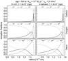 |
Fig. 3 Radial distribution of ionic fractions of carbon (top panels), oxygen (middle panels), and neon (bottom panels) inside the two bubbles shown in Fig. 2. Left column: PN composition, right column: WR composition. |
2.4 The characteristic X-ray temperature and line measurements
The characteristic temperature of the X-ray emitting plasma of a HB can be defined as
 (1)
(1)
Here, Te(r) is the electron temperature between inner bubble radius r1 (position of the reverse windshock) and outer bubble radius r2 (conduction front),
 (2)
(2)
is the X-ray luminosity, and
 (3)
(3)
is the volume emissivity in the energy band E1 − E2 (Eqs. (17)–(19) in Steffen et al. 2008). The temperature TX as defined here is the typical plasma temperature where most of the X-ray emission is generated. For our ZP96 bubbles, the radial temperature profile, Te(r), is determined by heat conduction.
The definition of TX in Eq. (1) implies that its value depends, via the emissivity, on the chemistry, even if the temperature profile is the same. However, another chemistry also implies a different conduction efficiency and hence a different temperature profile inside the bubble. This has been demonstrated in Fig. 2 above: the bubble with hydrogen-poor WR composition has a steeper temperature gradient because of its lower conduction efficiency, hence more matter (and emissivity) is concentrated towards the conduction front where the electron temperature is lower. Thus, according to Eq. (1), the bubble with WR composition has a lower TX value than the bubble with PN composition (cf. Fig. 2).
A similar effect occurs for bubbles with an inhomogeneous chemical composition: the value of TX depends on the position of the chemical discontinuity in bubbles where the inner region consists of original WR matter but the outer part consists of evaporated hydrogen-rich PN matter. The reason here is mainly the very different emissivities of the WR and PN elemental mixtures. Bubbles with inhomogeneous composition will be discussed in detail in Sect. 5.
We use appropriate line ratios to analyse our synthesised HB model spectra in terms of their TX values. As we start with a fully parametrised model, we know the HB temperature distribution and the chemical composition, either homogeneously hydrogen-poor or -rich or inhomogeneously with a chemical discontinuity.
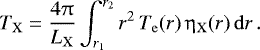
We alsoknow possible sources of line blending from the line list. As we wanted to test our model on BD + 30, we focused our line ratio measurements on features that have been observed or constrained by Yu et al. (2009, Table 2 therein). These lines are Mg XII, Mg XI, Ne X, Ne IX, O VIII, O VII, N VII, C VI, and C V (Table 3). In Fig. 4, we show the spectral windows of these lines. The spectral resolution was set to 0.001 Å for clarity, but in our analyses we applied aresolution of 0.01 Å, which is still about an order of magnitude finer than currently accessible by observations (Yu et al. 2009).
The line luminosity was determined by integrating over a 0.1 Å window around these lines to produce results similar to Chandra observations (Yu et al. 2009). The 0.01 Å resolution ensures that the line in question is properly resolved, while the choice of the0.1 Å integration window represents the lower spectral resolution provided by the Chandra LETG observations. Hence, the two Mg XII lines, the two Ne Xlines, the two O VIII lines, the two N VII lines, and the two C VI lines were not resolved. Throughout this paper, Fe XVII measurements refer to the centre Fe XVII line at 17.05 Å, because thisis the strongest emission line of this ionisation state. For Ne IX, we decided to work with the average of the two available lines, as they are of similar strength. Line centres are taken from the CHIANTI database.
Figure 4 illustrates that contamination by overlapping blend lines is an issue for the 0.1 Å Chandra spectral resolution. As an example, consider the left panel in the second row, where we target at the Ne X lines at 12.1321 and 12.1375 Å. In this high-resolution representation, we identify Ne IX d (12.1113 Å), Fe XVII (12.1230 Å), and a blend of Fe XXI* (12.1551 Å), Ni XX (12.1570 Å), Mn XXIII (12.1586 Å), Fe XXI* (12.1589 Å), and Fe XXIII (12.1612 Å), all of which contribute to our line measurement of the two Ne X lines7. Line blending will unavoidably lead to imprecise line ratio measurements, because this melange of ions is distributed over a range of HB radii, leading to different ionisation equilibria (see Fig. ??). When applied to observations with lower resolution (as in Yu et al. 2009), such values must be treated with caution if contamination is not discussed. In this particular case, we have verified that contamination under the Ne X multiplet around 12.13 Å is weak in the cases we consider. However, we note the logarithmic ordinate scale in Fig. 4.
 |
Fig. 4 Zoom-in on spectral windows of the CHIANTI output that were considered for our analyses. We note the logarithmic scale on the ordinate and the numerous contributing lines. Without loss of generality, the bubble used is that shown in the top panels of Fig. 2. The hydrogen-rich PN case has been chosen in order to highlight the N VII line, which is virtually absent for the WR composition. We show the spectra at different resolutions (see legend), the spectral range and resolution chosen for the line integration (red), the continuum (short-dashed), and the domains where the continuum is defined for the integrations (blue, on the abscissae). |
2.5 Properties of the ZP96 bubble models
In this sub-section, we will illustrate how the spectral appearance, and hence the line ratios, depend on the bubble parameters. All the models are assumed to have the WR chemical composition from Table 2. We selected the oxygen line ratio O VIII/O VII and plotted it in Fig. 5 over the characteristic X-ray temperature TX computed according to Eq. (1). Using all models listed in Table 1 (top left panel), we see that they degenerate into virtually one single sequence over TX, which allows us to determine a well-defined characteristic bubble temperature, independently of the choice of the parameter set.
Starting from a model with mean properties (as used in Fig. 2), the influence of changing age and slow-wind properties, both for three thermal conduction coefficients C, is illustrated in the other panels of this figure:
-
evolution with age, the slow-wind parameters fixed (top right);
-
evolution with Ṁsw, vsw and age fixed (bottom left);
-
evolution with vsw, Ṁsw and age fixed (bottom right).
First of all, we notice that a higher conduction efficiency leads to higher characteristic X-ray temperatures TX . For the temperature and conduction efficiency ranges considered here, the corresponding TX variation is limited to 0.4–0.5 MK.
The dependences on the other parameters are quite different, and their ranges for the respective parameter spaces are indicated by the areas labelled “I”, “II”, and “III” in the top left panel of Fig. 5. The most important parameter is, of course, the age (top right panel): between 200 and 1000 yr, and for the annotated slow-wind parameters, TX increases from about 1.3 to up to 3.25 MK. Next comes the slow-wind mass-loss rate (bottom left panel). For a variation from 10−7 to 10−4 M⊙ yr−1 at a given age, TX increases only by a factor of two, from about 1.3 MK to 2.7 MK. The influence on slow-wind speed is depicted in the bottom right panel of Fig. 5. For a reasonable velocity increase from 10 to 40 km s−1, TX decreases from 2.4 to 2.1 MK, only. All these results refer to the models with fixed parameters as indicated above each individual panel.
This general dependence of TX is evident from the solution given in Zhekov & Perinotto (1996, Eq. (12) therein) where one sees that TX is a monotonously increasing function of the density at the outer bubble boundary via “slow-wind” mass-loss rate and/or speed.
For application to real objects, the parameters discussed above have to be specified, at least in principle. The heat conduction parameter isfixed by the chemical composition, but the slow-wind parameters must be estimated from observations. We note that they are notto be confused with the values of the former slow AGB wind. Instead, we need the corresponding values ahead of the rim shock, those at the rim/shell interface. For the case of BD+30, Bryce & Mellema (1999) measured 28 km s−1 from [N II] and 36 km s−1 from [O III], respectively, which, however, are “mean bulk” velocities based on the line-peak separation. We assume that vsw is not far from either of these values. To get the value of Ṁsw, a detailed density and velocity model of the nebula of BD+30 is necessary but not yet available. We will see in the next section that the range of values used in Fig. 5 is representative.
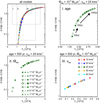 |
Fig. 5 Dependence of the bubble properties in terms of the line ratio O VIII/O VII (18.97 Å/21.60 Å) versus TX on age (panel I), and slow-wind properties (panels II and III). The fixed model parameters are indicated at the top of the respective panels. In each of these three panels, we distinguish between three values of the conduction parameter C: 3.0 × 10⁻⁷ (grey), 4.5 × 10⁻⁷ (open), and 6.0 × 10⁻⁷ erg cm−1 s−1 K7∕2 (filled), as indicated in the legends. Top left panel: all computed bubble models, and the annotated areas (I, II, and III) indicate the plot ranges shown in the respective panels I, II, and III. Without any loss of generality, we selected the WR model shown in Fig. 2, which is close to the middle of the parameter space listed in Table 1, as the reference model. The bubbles’ chemical composition corresponds to the WR case of Table 2. |
2.6 Single-temperature plasma models
For a comparison between our ZP96 models and the isothermal approach, we constructed bubbles with a constant electron temperaturein the following way. Given a ZP96 bubble with the typical heat-conduction temperature profile characterised by TX and a (constant) pressure p, a new bubble (“iso-HB”) with constant temperatureat the value of TX and a corresponding constant value of p was then constructed and its X-ray spectrum computed in the same fashion as before. These single-temperature bubbles also have a spatially constant density.
The run of the O VIII/O VII line ratio with TX predicted byour iso-HBs is also displayed in Fig. 6 and compared with the predictions of the ZP96 bubbles with both the WR (same as in Fig. 5) and PN composition. We note that the iso-HB predict line ratios independently of the plasma’s chemical composition. The iso-HB O VIII/O VII line ratio depends differently on TX , and this behaviour reflects the different radial temperature profiles: constant temperature (with accordingly constant ionisation fractions) versus heat-conduction temperature profile with stratified ionisation. Below TX ≈ 2.6 MK (WR) or TX ≈ 2.3 MK (PN), the bubble’s characteristic temperature is slightly overestimated; above, it is severely underestimated if a single-temperature plasma model is used for the interpretation of the O VIII/O VII ratio.
A qualitatively similar behaviour is found for the Ne X/ Ne IX line ratio, although the difference between the iso- and ZP96 HBs is higher, to the extent that the use of iso-temperature models always leads to an overestimate of the characteristic plasma temperaturebelow about 4.5 MK.
The difference between bubbles with WR and PN compositions has already been explained (Sect. 2.2) in conjunction with the definition of TX according to Eq. (1). In general, at a given O VIII/O VII line ratio, the PN bubbles have a higher TX value, but the degree of this difference depends on the value of the line ratio. At the lowest line ratios, that is, very young bubbles, the difference virtually vanishes, but it increases steadily and becomes eventually more than 2 MK for the 1000-yr old models.
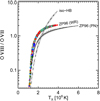 |
Fig. 6 Same as in the top left panel of Fig. 5 but now including also bubble models with hydrogen-rich PN-matter (symbols with black central line, C = 6.0 × 10⁻⁷ erg cm−1 s−1 K7∕2), and single-temperature bubbles (iso-HB, small triangles). |
3 The applicability of the ZP96 bubbles
One of the necessary assumptions to compute the structures of heat-conducting bubbles analytically is the neglect of radiative cooling. The influence of heat conduction is twofold:
- 1.
a possible steepening of the temperature gradient towards the conduction front, and
- 2.
a delay in bubble formation.
The first item affects only the outermost, coolest layers close to the conduction front where the density (and hence cooling) is highest. However, once the bubble is formed, densities are low and the cooling timescale becomes long, whereas heat conduction has an “instantaneous” effect on the bubble structure (ZP96). We therefore do not expect any significant effect on the bubble structure (radial temperature and density profile) by neglecting radiative cooling.
Concerning the second item, radiative cooling is quite important. While our ZP96 bubbles form immediately at age zero (with very small wind speed), the formation of a hydrodynamical bubble is postponed by radiative cooling until the cooling time exceeds the “crossing time” of the free wind (see e.g. discussion in Mellema & Lundqvist 2002). For normal PN matter, this delay is modest and corresponds to a wind speed of about 170 km s−1 according to Kahn & Breitschwerdt (1990), which has been confirmed by the radiation-hydrodynamics models of Perinotto et al. (2004). Heat conduction has only a minor impact on formation and evolution of a wind-blown bubble (cf. Fig. 4 in Steffen et al. 2008).
For hydrogen-deficient and carbon-rich matter, radiative cooling is much more efficient, and a wind-blown bubble does not form before the wind speed reaches about 500 km s−1, heat conduction not included (Mellema & Lundqvist 2002). Our detailed radiation-hydrodynamics simulation with heat conduction reveals an even later development of a bubble formed out of a hydrogen-poor, carbon-rich wind (Paper I). Wind speeds of about 1000 km s−1 (corresponding to Teff ≃ 50 000 K) are required to overcome the very efficient radiative cooling caused by the higher bubble densities (orders of magnitude) in the heat-conducting case.
Despite these differences between analytical and hydrodynamical X-ray bubbles, the application of the ZP96 bubbles to the analysis of the X-ray spectrum of real bubbles is still possible provided the analytical bubbles are comparable in size and X-ray luminosity to the bubble of BD +30. The nebula of BD +30 has a kinematical age of about 800 yr (Li et al. 2002), thus the nebula is rather young and quite small, and so is also an X-ray emitting bubble8 . With a distance to BD+30 of 1300 pc, the bubble radius is 0.013 pc, or 4 × 1016 cm (cf. Kastner et al. 2008)9. Based on this distance, Ruiz et al. (2013) estimated an X-ray luminosity of about 2.7 × 1032 erg s−1. From their high-resolution observations, Yu et al. (2009) determined an X-ray luminosity (7.4–8.6) × 1032 erg s−1 for a distance of 1200 pc. The lower luminosity given in Ruiz et al. (2013) goes back to Kastner et al. (2000) and is based on a much lower column density of intervening matter than found by Yu et al. (2009). From cuts along the minor axis using Hubble Space Telescope images of BD +30, one can estimate a relative rim thickness of Δ θrim∕θrim ≃ 0.15−025 (full width at half maximum), just about the limit for justifying the thin-shell approximation for the expanding bubble/rim system of BD +30.
Figure 7 illustrates the ranges in size and X-ray luminosity of our ZP96 bubbles with WR composition. The ages run from 200 up to 1000 yr with monotonously increasing X-ray luminosities. Furthermore, LX increases with Ṁ sw and decreases with the flow velocity vsw, that is, it increases with upstream density, as indicated by the arrows in the figure. Middle-aged (300–600 yr) bubbles with low Ṁ sw and relatively high vsw cover well the observed bubble parameters for BD +30 with respect to size and X-ray luminosity. At the lowest slow-wind mass-loss rates and highest slow-wind velocities, the assumptions inherent to the analytical solutions (see Sect. 2.1) break down for higher ages, and the models are thus not shown in Fig. 7.
4 Resultsfor BD +30° 3639
In this section, we re-analyse the existing flux-calibrated (in photons cm−2 s−1) high-resolution X-ray line spectrum of BD+30 published in Yu et al. (2009) by means of the bubble models presented in the previous sections. The line photon fluxes listed in their Table 2 have to be converted into units of erg s−1Å−1 by
 (4)
(4)
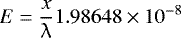
(Allen 1976), where E (in erg s−1) is the line luminosity (that is, the area under the red segment in a line shown in Fig. 4), x is the number of photons per second (e.g. from Table 2 in Yu et al. 2009), and λ is the wavelength in units of Å10.
We assume in a first approximation that all ZP96 bubbles have the homogeneous WR composition listed in Table 2, which means that they are devoid of “evaporated” PN matter. We emphasise that the assumption of a homogeneous chemical composition of the emitting plasma, whether normal or more “exotic”, is the standard assumption used in all analyses of the X-ray emission from wind-blown bubbles conducted so far.
A general uncertainty in all plasma studies in the X-ray regime is the amount of absorption by intervening matter, characterised by the neutral hydrogen column density NH. In the case of BD +30, the situation is even more complicated. The absorption appears to be variable across the bubble’s image (Kastner et al. 2002). Given this situation, it is not astonishing that the value of NH varies considerably from study to study, as listed in Table 4 of Yu et al. (2009, and references therein). The value of NH varies between 0.10 × 10²² and 0.24 × 1022 cm−2, depending on the method used. The low values around 0.10 × 1022 cm−2 are from optical data converted to NH, whereas higher values of NH are determined simultaneously with the other plasma parameters by matching one-temperature plasma models to the observations.
The task that we have to solve by comparing our heat-conducting ZP96 bubble models to the X-ray emission of BD +30’s hot bubble is then the following:
-
determine the amount of intervening absorbing matter, NH;
-
fix the characteristic bubble temperature TX;
-
get abundance ratios for the main constituents of the bubble; and
-
derive the amount of evaporated hydrogen-rich nebular matter, if any.
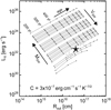 |
Fig. 7 X-ray luminosity (5–40 Å, 0.3–2.5 keV) versus bubble size for the bubble sub-grid with WR composition and C = 3 × 10⁻⁷ erg cm−2 s−1 K−7∕2, and for ages from 200 to 1000 yr. Black dots indicate individual bubble models. The slow wind, Ṁ sw , ranges from 10−7 to 10−4 M⊙ yr−1, the slow-wind velocity, V sw, from 10 to 40 km s−1 (cf. Table 1). The adopted values for BD +30 (see text) are marked by the filled star. The open stars indicate the positions if the assumed distance to BD +30 is increased or decreased by a factor of two. |
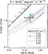 |
Fig. 8 Line ratio of O VIII/O VII over line ratio Ne X/Ne IX for BD +30 (error cross) after Yu et al. (2009, Table 2) and for ZP96 heat-conducting bubbles with homogeneous hydrogen-poor WR composition subject to various absorptions as indicated in the legend. Individual models are only shown for NH = 0 (circles) and NH = 0.20 × 1022 cm−2, the value adopted (grey dots). For other values of NH, only envelopes are given in order to avoid confusion. Evolution proceeds from low to high line ratios, that is, from low to high TX. The oldest (1000 yr) and hottest (4 MK) bubble models always have neon line ratios of about 2, virtually independent of NH. The crosses are the models that lie within BD +30’s error box. The filled square (green) marks our “best-fit” bubble model, presented in Sect. 4.3. The filled triangles are bubbles with constant temperatures (iso-HB, for NH = 0.20 × 1022 cm−2 only, see text for details). The numbers along the iso-HB sequence indicate the bubble temperatures in MK. |
4.1 The column density NH and the characteristic temperature TX
We follow the method of determining the column density of the intervening matter from the X-ray spectrum itself. However, since the extinction is wavelength dependent, it happens that abundance ratios, for example of C/O, derived from lines with considerable wavelength separation do depend on the chosen value of NH . In other words, abundance ratios cannot be determined independently of NH .
Therefore, we used abundance-independent line ratios for the NH determination. In order to be consistent with Yu et al. (2009) for the wavelength-dependent absorption of our model spectra, we applied the standard, solar abundance model of Morrison & McCammon (1983). Our method for deriving NH is illustrated in Fig. 8, where the absorbed temperature-sensitive line ratios O VIII/O VII and Ne X/Ne IX of our bubble models are compared with BD +30’s observed line ratios. These line ratios are independent of the abundances, but unfortunately not very sensitive to the value of NH because of the rather small wavelength separation of the employed lines. Nevertheless, we believe that this is the only acceptable method for high-resolution spectra because chemical abundances are, in principle, not known a priori.
According to Fig. 8, the line ratios are changed by the amount of intervening gas such that all models are shifted upwards with increasing NH , that is, only the O VIII/O VII line ratio is really sensitive to NH. The models with NH = 0.20 × 1022 cm−2 (grey dots) match the observation best, and the cloud of 32 crosses marks the bubbles whose oxygen and neon line ratios are within BD +30’s error box. Lower and higher values of NH appear to be acceptable as well, and we adopt  , a result which is, within the errors, consistent with the determinations of Yu et al. (2009) and Nordon et al. (2009) of NH= (0.24 ± 0.04) × 1022 cm−2. The extinction in the visible is reported to be AV ≃ 1 mag, which then corresponds to NH ≃ 0.22 × 1022 cm−2 if the conversion of Gorenstein (1975) is employed.
The 32 bubble models marked by crosses in Fig. 8 have quite different ages, sizes, and X-ray luminosities and may not always fit the observed parameters of BD +30’s bubble. We thus selected models that comply with the following criteria for luminosity and size: LX ≃ 1032−1033 erg s−1 and Rout ≃ 2 × 10¹⁶…8 × 1016 cm, which embrace approximately the observed values for the bubble of BD +30 (cf. Fig. 7). With these constraints, we are left with ten bubble models in the range of 1.68–1.89 MK, and we adopt TX = 1.8 ± 0.1 MK for the bubble of BD +30, a value nearly independent of NH. This TX value corresponds well with that of Yu et al. (2009) who found 1.7 ± 0.4 MK for the low-temperature plasma component.
The iso-HBs are also plotted in Fig. 8 (filled triangles), but only for the NH= 0.20 × 1022 cm−2 case because the dependence on NH is similar. The positions of these bubbles with respect to the observations confirm the conclusion of Yu et al. (2009) that plasma models with a single temperature are unable to describe the X-ray emission of BD +30’s bubble adequately. However, we need iso-HBs with rather high temperatures of 2.3 ± 0.2 and 2.9 ± 0.3 MK to match the observed O VIII/O VII and Ne X/Ne IX line ratio, respectively (Fig. 8). We consider it a real success of our analytical ZP96 bubbles with heat conduction that they match both the oxygen and neon line ratios with a single value of TX.
For completeness, we considered also other temperature-sensitive line ratios, C VI/C V and Mg XII/Mg XI, although Yu et al. (2009)’s measurements are very uncertain (Mg) or constrained by an upper limit (C V). The magnesium lines trace the hottest ( ≃ 10 MK, see Fig. ?? ), innermost region of a bubble, and the failure of our ZP96 bubbles to match the observation despite their large errors (Fig. 9, left panel) could mean that
-
the innermost part of BD +30’s bubble is hotter than our models predict; or that
-
the measurements are more uncertain than expected, most probably because of blending.
The region immediately behind the wind shock can be hotter in reality than our ZP96 bubbles predict because the (standard) heat-conduction formulation may break down there due to heat-flux saturation (Cowie & McKee 1977). This possibility has been discussed in some detail in Steffen et al. (2008) in conjunction with the numerical treatment of thermal conduction.
For the carbon line ratio, which is sensitive to the region behind the conduction front, there appears no conflict between model predictions and the observation (right panel of Fig. 9).
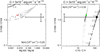 |
Fig. 9 Sameas in Fig. 8 but now for O VIII/O VII over Mg XII/Mg XI (left panel) and over C VI/C V (right panel), and only for NH = 0.20 × 1022 cm−2. The symbols have the same meaning as in Fig. 8. The position of the “best-fit” models is either the filled (green, rightpanel) or crossed square (left panel). |
4.2 On the chemical composition of BD +30’s hot bubble
In general, any abundance analysis of X-ray spectra suffers from the fact that the two usually most abundant elements, hydrogen and helium, are unobservable. Instead, one has to make reasonable assumptions about the abundance of these two elements, otherwise only abundance ratios can be derived. In the case of a wind-blown bubble inside a planetary nebula with a hydrogen-poor or -free [WR] central star, it appears justified to assume that all or at least most of the bubble also contains the hydrogen-poor material from the stellar surface. This is especially important for the bubble of BD +30 because it is already clear from its low-resolution X-ray spectrum that the bubble plasma must be extremely enriched in carbon and neon. With this in mind, one has to accept that the absolute abundance values deduced for BD +30’s bubble by Yu et al. (2009) and Nordon et al. (2009) are not meaningful.
The chemical composition of our ZP96 bubbles is given by the WR mixture listed in Table 2, which in turn is based on the work of Marcolino et al. (2007) in which photospheric or wind lines of the central star have been analysed in detail. As already mentioned in Sect. 2.2, only He, C, and O are provided by the above authors, and the abundances of the other elements, especially those of Ne and Mg, have been assumed by us. Since hydrogen and helium lines are not observable in the X-ray range, only abundances relative to, for example, oxygen, can be derived. We use the O VIII (recombination) line 18.97 Å as representative for oxygen because O8+ is the dominant ion inside the bubble, except close to the conduction front where temperatures are too low (cf. Fig. 3). This line is thus not very sensitive to possibly evaporated matter near the conduction front that has a different oxygen content (for instance hydrogen-rich PN matter).
Neon, magnesium, and silicon
We illustrate in Fig. 10 how the abundances of neon and magnesium relative to oxygen can be derived. We begin with magnesium (left panel) because we see in Fig. 9 above that our ZP96 models fail to reproduce the observed Mg XII/Mg XI line ratio. First of all, only the hottest models with TX ≳3 MK can match the observed Mg/O line ratios. However, these models are far from the observed line ratios in Figs. 8 and 9 (left). Increasing the magnesium abundance does not help either: factors between 2 and 32 provide consistency with the observed Mg XI/O VIII line ratio. A factor of about ten corresponds to the solar Mg/O reported by Yu et al. (2009) and Nordon et al. (2009). The observed Mg XII/O VIII line ratio, however, remains unreachable. A reliable magnesium abundance cannot be determined, and we thus do not consider Mg any further.
The situation is much better for neon, although our bubble models also fail to match the neon/oxygen line ratios. However, an increase of our initial neon abundance by factors between only 1.5 and three give good agreement with the observations. We assume  . Yu et al. (2009) derived
  , in reasonable agreement with the observations11. The neon abundance drawn from the diagram used in Fig. 10 is not very sensitive to the value of NH : even assuming no absorption, the factor increases by about 50% only.
The situation for silicon is similar to that for magnesium. The silicon abundances rest on one very weak line ofSi XIII, and Nordon et al. (2009) found (also corrected for the solar oxygen abundance)  , which is about 1/8th of their neon-to-oxygen ratio. We cannot confirm this finding, as Fig. 11 shows. We see that the silicon abundance used by us must be increased by about a factor of ten, at least. However, taking the observed Si XIII/O VIII line ratio at face value, we arrive at (Si/O)BD ≈ 100 ×
  that is, silicon would be about as abundant as neon, which is difficult to understand.
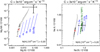 |
Fig. 10 Absorbed line ratios of Mg XII/O VIII over Mg XI/O VIII (left panel) and Ne X/O VIII over Ne IX/O VIII for NH = 0.20 × 1022 cm−2 and the resp- ective observed line ratios for BD +30 (error cross). The symbols have the same meaning as in Fig. 8 (or Fig. 9). The parallel lines indicate the shift of the crossed models (and the “best-fit” model as well) if the original bubble abundances of Mg (left panel) or Ne (right panel) are multiplied by the given factor. The corresponding shifts of the remaining bubble models are not shown in order to avoid confusion. |
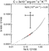 |
Fig. 11 Same as in Fig. 8 but for Si XIII/O VIII over Ne X/O VIII and for NH = 0.20 × 1022 cm−2. The grey dots and crosses mark the sequence of our ZP96 bubbles with the new, enhanced neon abundance; the crossed square indicates the “best-fit” model. |
Carbon
Although the abundance of carbon (or C/O) inside the hot bubble of BD +30 is given by the central star’s photospherical composition, the study of the carbon lines accessible in the X-ray regime (C V and C VI) is interesting in principle. The carbon lines are sensitive to extinction thanks to their rather high wavelengths, and carbon gets fully ionised close behind the conduction front (see Fig. 3). Because of the latter property, the C V line (not useful here) and also the C VI lines are immediately influenced by even small amounts of evaporated matter with a different, normal, carbon content.
Now the question to be answered is whether the oxygen/carbon and neon/carbon line ratios are consistent with the respective photospherical abundance ratios for the derived value of NH . If not, it means that either the amount of absorption has been wrongly chosen or hydrogen-rich matter has evaporated into the bubble.
The case is illustrated in Fig. 12 where the necessary increase of the neon abundance (see Fig. 10, right panel) has already been taken into account. We see that most our ZP96 bubbles selected on the basis of Fig. 8 are consistent with the observations, which can be interpreted such that the bubble of BD +30 still has the hydrogen-deficient WR composition of the stellar photosphere. Evaporated hydrogen-rich nebular gas is either not present or its amount is still too small to be observed. We will come back to the latter point in the next section.
Yu et al. (2009) derived a C/O ratio of  and Nordon et al. (2009) from the same data
 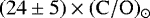 , both values again corrected for the lower solar oxygen abundance of ϵ = 8.73. The carbon/oxygen ratio of the WR mixture used by us is 12 (by number, Table 2). Thus, we have
  , in good agreement with the findings of Yu et al. (2009) and Nordon et al. (2009). We remark that also in this case the iso-HB models are unable to match both the observed O VIII/C VI and Ne X/C VI line ratios with a single temperature (Fig. 12).
We mentioned already in Sect. 2.2 that the analysis of Crowther et al. (2006) provided a somewhat different chemistry at the stellar surface of BD +30 than that given by Marcolino et al. (2007) that we have used here. Helium and oxygen are higher at the expense of carbon, which has now a mass fraction of 0.38 only. Specifically, the oxygen abundance is nearly doubled, from 0.06 (0.05 from Leuenhagen et al. 1996) to 0.10 (mass fractions). These changes of the carbon and oxygen abundances lead in Fig. 12 to the following shift of the bubble positions: about 0.4 dex upwards and about 0.1 dex to the right. Consequently most of the crossed models (including the “best-fit” model selected below) will leave the error box.
Even more disturbing is the fact that, because the Ne/O abundance ratio is fixed by the observation (cf. Fig. 10, right panel), the neon mass fraction nearly doubles as well and becomes 0.09, an unreliably high value. Mainly for the latter reason, we do not consider the Crowther et al. (2006) abundances any further. We must consider, however, that a carbon abundance that is lower, for example, by about 10% than the one used here would give an even better match to the observations. Alternatively, a small increase of NH to 0.22 × 1022 cm−2 would do the same job without violating the constraints set by Fig. 8.
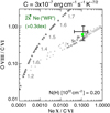 |
Fig. 12 Same as in Fig. 8 but for O VIII/C VI over Ne X/C VI and for NH = 0.20 × 1022 cm−2. The neon abundance from Table 2 (WR) is increased by a factor of two. The horizontal shift of the bubbles from their original positions is indicated by the error in the upper left corner of the plot. The green square marks our “best-fit” bubble (see text). Filled triangles represent our iso-HB models, also shifted accordingly. |
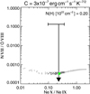 |
Fig. 13 Upper limit of the observed line ratio N VII/O VIII versus Ne X/Ne IX compared to the model prediction. Symbols have the same meaning as in the previous figures. |
Iron
We refrain from deriving the iron abundance because Yu et al. (2009) give only upper flux limits. Nevertheless, a Fe/O abundance ratio of about 0.1 solar was deduced and an iron deficiency claimed. We comment that the low Fe/O abundance ratio is more likely due to the highly increased oxygen abundance and not to an iron deficiency (cf. discussion in Sect. 2.2).
Nitrogen
Knowing the abundance of nitrogen is crucial because it is a tracer of BD +30’s previous evolution. We mentioned in Sect. 2.2 that we assume complete hydrogen and helium burning of nitrogen to neon after which the intershell matter becomes exposed. If such a scenario for the evolution of BD +30 is correct, the strong N VII at 24.8 Å line should be missing because our ZP96 models predict an N VII/O VIII line ratio of well below 10−3 for our WR mixture with an N/O abundance ratio (by number) of 2 × 10⁻⁴ (see Fig. 13).
We note that Yu et al. (2009) and Nordon et al. (2009) derived  and
and  , respectively,which is consistent with our assumption of virtually no nitrogen at all. Looking at the Chandra LETG spectra of BD +30’s hot bubble that are publicly available 12, we estimated a line flux ratio N VII/O VIII of about 0.13, provided the weak feature seen at 24.8 Å is really the N VII line. We use this value in Fig. 13 as an upper limit. Taken at face value, this upper line-ratio limit would roughly correspond to a nitrogen mass fraction in the WR mixture of 0.003, close to the (about solar) nitrogen mass fraction in the PN mixture.
The upper limit for the bubble’s nitrogen content is not helpful in clarifying the evolutionary history of BD +30. A better constraint of the nitrogen abundance is urgently needed so that a distinction between the different possible scenarios discussed in Sect. 2.2 can be made.
Parameters of the “best-fit” bubble model and observed values of BD +30° 3639’s hot bubble.
4.3 Our “best-fit” model
We have seen in Figs. 8 and 12 that quite a number of model bubbles satisfy the temperature-sensitive line ratios of oxygen and neon in conjunction with the abundance sensitive carbon/oxygen and carbon/neon line ratios. Without loss of generality, we selected a ZP96 bubble that is a compromise between Figs. 8 and 12 and is close to the error-cross centres of these figures: our “best-fit” bubble model (filled green square). The parameters of this model are listed in Table 4.
We see from Table 4 that size and X-ray luminosity of the “best-fit” model lie well within the limits given by observations (cf. Fig. 7). However, we emphasise again that some of the parameters in Table 4, like those that describe the outer boundary conditions (Ṁ sw, vsw ), have no relation to the actual situation of the nebular system of BD +30. Other combinations of Ṁ sw and vsw are equally possible, but not listed here. The only fitted parameters are TX and the abundance ratio of Ne/O, which is then used to derive the neon abundance mass fraction by employing the input abundances from the WR mixture used in the computations.
We notethat we cannot make any statement on the hydrogen content of BD +30’s bubble. The finite hydrogen content of the “best-fit” bubble listed in Table 4 is only meant as an upper limit based on analyses of BD +30’s stellar spectrum in the optical wavelength region (e.g. Leuenhagen et al. 1996). Most likely, the bubble of BD +30 is completely hydrogen-free.
5 Bubbles with inhomogeneous chemical composition
The mass budget of a HB with heat conduction is controlled by two contributions: stellar wind matter from within passing through the reverse shock and gas from the environment “evaporating” through the conduction front (cf. Borkowski et al. 1990). In the framework of ZP96 it is implicitly assumed that the chemical composition is homogeneous throughout the HB; that is, that it is either hydrogen-rich (the normal case) or hydrogen-deficient (as assumed here so far).
However, we know from observations that planetary nebulae with [WR]-type central stars do not share the stellar abundance peculiarity of being hydrogen-poor and carbon-rich (see e.g. Girard et al. 2007). Instead, the nebula chemistry is hydrogen-rich and indistinguishable from nebulae around normal, hydrogen-rich central stars. Therefore, ifwe want to model realistic bubbles, we have to consider that the evaporated gas is hydrogen-rich, that is, with PN chemistry. Depending on the age of the HB, a certain fraction of the bubble’s outer mass shells behind the conduction front should consist of hydrogen-rich nebular gas heated and evaporated across the conduction front.
In the following, we introduce and discuss heat-conducting bubbles that have an inhomogeneous (or stratified) chemical composition, in which the outer bubble region consist of hydrogen-rich PN matter while the remaining inner parts still have the original hydrogen-poor WR composition.
5.1 Construction and properties of wind-blown bubbles with inhomogeneous chemical composition
We constructed chemically inhomogeneous bubbles in the following way. Beginning at the conduction front and keeping temperaturedistribution and pressure within the ZP96 bubble constant, we replaced shells of hydrogen-deficient WR composition with shells of hydrogen-rich PN composition. In order to speed up the analysis and since (i) changes are expected to be most pronounced for shells with steep temperature gradients, and (ii) BD+30 as a young object is expected to have still a limited amount of evaporated H-rich matter, we set the positions of the chemical discontinuity such as to form a geometric sequence (illustrated by dots along the abscissa in Fig. 14).
Keepingthe temperature distribution unchanged implies also no change of the conduction efficiency across the chemical discontinuity. Since the fraction of evaporated hydrogen-rich matter for the hot bubble of BD +30 is expected to be very small, if any at all, we generally kept the value of the heat efficiency constant as is valid for the hydrogen-poor WR mixture: C = 3.0 × 10⁻⁷ erg cm−1 s−1 K7∕2. Additionally, we also considered bubbles with an intermediate value, C = 4.5 × 10⁻⁷ erg cm−1 s−1 K7∕2. In any case,as we have seen above (Fig. 5, upper right panel), the value of C has only a rather modest influence on the bubble temperature TX and the corresponding temperature-sensitive line ratios.
How realistic is the assumption of a sharp discontinuity (or density jump) at the transition between both sets of compositions? Our 1D hydro models suggest a rather sharp transition region that is quite small compared to the bubble size (middle panel of Fig. 7 in Paper I). Whether dynamical instabilities will break completely any chemical discontinuity set up by evaporation cannot be answered at present.
Our bubble modelling also ignores the time evolution during which the bubble mass increases by the evaporated gas. Instead, here we are only replacing the WR with PN matter. Nevertheless, as we will see below, chemically stratified bubbles constructed in this way can well be used as a diagnostic tool to investigate the line emission of chemically stratified wind-blown bubbles and to address the question of whether heat conduction with concomitant PN-matter evaporation is at work and how large the mass fraction of the evaporated PN matter really is.
As an example of our modelling, we show in Fig. 14 the physical structure of a chemically stratified bubble of intermediate age with a 3% mass fraction of PN matter: ω ≡ MPN∕(MWR + MPN) = 0.03. One sees clearly that the condition of constant pressure in conjunction with the different element mixture leads to a jump of electron and ion densities at the position of the chemical discontinuity.
Because we have seen that hydrogen-rich and hydrogen-poor compositions have very different X-ray emission properties (Fig. 2), a stratified chemical composition has a profound influence on the bubble’s X-ray emission, which is illustrated in the following two figures. Figure 15 shows how the X-ray surfaces brightness (or intensity) changes with the position of the chemical transition, while the other bubble parameters remain unchanged. Since the emissivity of the hydrogen-rich matter is much lower, the composition transition is marked by a huge intensity drop of up to two orders of magnitude, depending on the radial position of the WR–PN matter transition. Correspondingly, the total X-ray luminosity decreases rapidly if the WR–PN discontinuity moves inwards. The case of a purely hydrogen-rich bubble cannot be achieved in nature because the stellar wind continuously feeds new WR matter into the bubble.
Figure 16 illustrates how the X-ray spectrum depends on the position of the chemical discontinuity but with otherwise unchanged structural parameters. The top-left panel displays the chemically homogeneous WR case (ω = 0.0), while the middle-left panel shows the spectral luminosity distribution for the ω = 0.03 case rendered in Figs. 14 and 15. The spectrum where the chemical dicontinuity is placed even further inside (ω = 0.15) is displayed in the bottom-left panel. Important emission lines are indicated above the panels, and the corresponding high-resolution profiles are shown in the 3 × 3 matrix of panels on the right.
The contamination by evaporated hydrogen-rich matter lowers the continuum emission of the bubble, preferably at longer wavelength where the emission of the cooler hydrogen-rich PN-matter immediately behind the conduction front dominates. For ω = 0.15, this effect is alsoapparent at shorter wavelenghts.
The influence of the position of the chemical discontinuity on the total line emission is seen in the 3 × 3 panel matrix on the right part of Fig. 16. The ionisation stratification imposed by the temperature gradient inside the bubble leads to line changes depending on the charge of the ion in question. The C V line nearly disappears for ω = 0.15, while neon and magnesium lines remain virtually unchanged. The oxygen lines behave intermediately in the sense that the O VIII line is much less dependent on the amount of hydrogen-rich PN matter.
The N VII line emission at 24.78 Å which is, of course, absent in the ω = 0.0 case, is very interesting. However, even a small contribution of PN matter (here 3%) makes this line visible (top-right panel in Fig. 16). Obviously, N VII is a sensitive tracer of the contamination of originally hydrogen-deficient and nitrogen-free bubbles with hydrogen-rich matter by, for example, heat-conduction-driven evaporation.
From the intensity distributions shown in Fig. 15, it is evident that although the bubble’s temperature distribution remains unchanged, the characteristic X-ray temperature TX , as computed according to Eq. (1), does depend on the position of the chemical transition. The reasons are the differentemissivities of the WR and PN matter. If the WR matter is replaced by hydrogen-rich PN matter with its lower emissivity, the weighting in Eq. (1) is more towards the inner, hotter regions, hence TX increases. While the position of the chemical transition moves inwards, TX will go through a maximum since at some point the emission of the inner hydrogen-deficient bubble regions begins to decrease because of the low densities and falls below that of the hydrogen-rich outer regions. Finally, TX drops to the value for a chemically homogeneous hydrogen-rich bubble.
This behaviour is illustrated in Fig. 17, where the run of the X-ray temperature versus the mass fraction of hydrogen-rich matter, ω = MPN∕(MPN + MWR), is shown fora suite of originally pure WR bubble models that satisfy the observed oxygen and neon line ratios (crosses in Fig. 8). One sees that very small fractions of PN matter (ω ≲ 0.005) do not change the X-ray spectrum, that is also TX, at all. These mass shells are obviously still too cool to emit significantly in the soft X-ray range. However, then TX increases from below 2.0 MK to well above 3 MK (up to 3.5 MK) for ω ≃ 0.2–0.3. For larger fractions of PN matter, TX decreases again somewhat, but even for the pure PN case, TX is higher than for the pure WR case (cf. Fig. 6 and discussion concerning the behaviour of TX in Sect. 2.4). In contrast, the X-ray luminosity decreases steadily with ω, as seen in the bottom panel of Fig. 17 (cf. also Fig. 15).
The strict correlations between temperature-sensitive line ratios and TX as shown in Figs. 5 and 6 no longer exist for chemically stratified bubbles. Instead, these line ratios depend on the position of the chemical transition and the abundance differences on both sides of this transition, as we will see in the next section.
We emphasise that the curves in both panels of Fig. 17 are not evolutionary sequences because the bubble masses increase steadily by evaporation and wind input. In reality, the dependance of TX and LX on ω is different and can only be determined by hydrodynamical simulations. Cases with ω ≃ 1 can certainly not occur in nature.
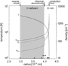 |
Fig. 14 Physical structure of a ZP96 bubble of age = 500 yr with a stratified composition such that ω ≡ MPN∕(MWR + MPN) = 0.03, with MWR = 5.59 × 1028 g and MPN = 1.67 × 1027 g, and with C = 3 × 10⁻⁷ erg cm−1 s−1 K7∕2, Ṁ sw = 5.0 × 10⁻⁷ M⊙ yr−1, and vsw = 25 km s−1. Shown are radial runs of electron, ion, total particle densities, and temperature. The central star is at the origin (radius = 0 cm), the wind reverse shock (= inner bubble boundary) is at 2.97 × 1016 cm, and the planetary nebula proper adjacent to the heat conduction front at 4.18 × 1016 cm. The compositions are those listed in Table 2: WR for hydrogen-deficient (grey) and PN for hydrogen-rich. The chemical discontinuity is at 3.98 × 1016 cm, or 2.0 × 10⁶ K. We note the logarithmic ordinate scales and the linear abscissa. For the meaning of the dots along the abscissa, see Fig. 15. See also Sect. 5.1 for details. |
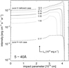 |
Fig. 15 Intrinsic intensity distributions of X-ray emission between 5 and 40 Å for the bubble used in Fig. 14 but with the chemical discontinuity located at different bubble radii, hence with different ω. The individual intensity distributions correspond either to the specific bubble model of Fig. 14 (solid) or to the positions of the chemical discontinuities being at radii indicated by the filled circles in Fig. 14 (dotted), whereas the two chemically homogeneous cases PN and WR are rendered as dashed lines. The model belonging to the open circle in Fig. 14 is not shown because of its similarity to the ω = 0.03 model. The numbers at the curves indicate the X-ray luminosities (in 1032 erg s−1 ) computed for the given wavelength range. |
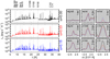 |
Fig. 16 X-ray spectral luminosity (left panels) and selected lines zoomed-in (right panels) of ZP96 bubbles with homogeneous WR composition (ω = 0.00, solid/black) and inhomogeneous WR + PN composition (ω = 0.03, dashed/red, and 0.15, dotted/blue). All three bubble models have the same dimension and temperature profile, and the one used in the middle-left panel is the model used in Figs. 14 and 15. The line-profile panels (grey) cover the wavelength range of 0.10 Å each (i.e. the Chandra resolution), but the (logarithmic) ordinate range may be diffferent so as to give a better match to the various line strengths. Also, all lines are normalised to a single continuum level to ease comparison. |
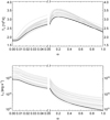 |
Fig. 17 Characteristic X-ray temperature TX (top panel) and X-ray luminosity LX (bottom panel) for a suite of chemically stratified heat-conduction bubbles constructed from pure WR ZP96 models that comply with both the observed oxygen and neon line ratios of BD +30 (crosses in Fig. 8) versus ω = MPN∕(MPN + MWR). The thick line corresponds to the model sequence originating from the 500-yr old “best-fit” WR-model. We note the break of the abscissa scale at ω = 0.05. The wavelength range considered is 5–40 Å (0.3–2.5 keV.) |
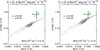 |
Fig. 18 Same as in Fig. 12 but for bubble models with lower absorptions as indicated in the respective panels. Filled circles give the positions of the bubbles with homogeneous WR composition (ω = 0 ) that comply with the constraints from Fig. 8 with the appropriate NH value. The green lines enclose the corresponding positions if in the outer bubble parts the WR mixture is replaced by PN mixture (ω = 0.03, left panel, and ω = 0.02, right panel). |
5.2 Constraints on the hydrogen-rich matter content of the hot bubble of BD +30
In this sub-section, we apply our grid of chemically stratified HBs to estimate the degree of chemical stratification within the young X-ray-emitting hot bubble of BD +30. From our findings discussed above, three methods are, at least in principle, suited for this purpose:
- 1.
Measuring a possible sharp radial drop in the X-ray intensity distribution as seen in Fig. 15. However, the rather low numbers of X-ray photons typical for existing observations of the objects in question do not allow such kind of measurements.
- 2.
The N VII line at 24.78 Å is obviously a very sensitive indicator. It is virtually absent in the spectrum of a pure WR composition as used here, but strong in the spectrum of a bubble with hydrogen-rich composition (cf. Fig. 16). If BD +30 belongs to the class of [WR]-type central stars that show photospheric nitrogen, the N VIIline at 24.78 Å should not be used at all as an indicator of element stratifications within wind-blown bubbles.
- 3.
Because of the ionic stratification caused by the heat conduction temperature profile (see Fig. 3), the reaction of the line strengths while the chemical discontinuity moves inwards depends on the degree of ionisation of the respective ions. Lines coming from ions with low degree of ionisation change early (e.g. C V and C VI lines), those originating from ions with high degree of ionisation later (e.g. O VIII and Ne X lines).
Since the methods under items one and two cannot be used for BD +30 because of the limited data quality, we are left with the facts described under item three and employ a diagram as shown in Fig. 12which has been used above to estimate the carbon abundance of BD +30’s bubble. Because of the relatively large wavelength separation of the used lines, such a diagram is sensitive to the selected hydrogen column density NH , and Fig. 18 gives two examples for smaller NH than used in Fig. 12.
This figure shows how sensitive the positions of the bubble models are to the chosen value of NH . For the low value of only 0.10 × 1022 cm−2, our ZP96 bubbles with homogeneous WR composition fail completely to explain the observations. For the higher value of 0.15 × 1022 cm−2, they just touch the error box. In both cases, chemically stratified models, constructed from the ω = 0 models in the manner described in the previous section, perform better. The C VI line emission gets weaker because of the lower line contribution from the PN matter (cf. Fig. 16, right grey panels), and the inhomogeneous models are shifted to the right and upwards in diagrams as shown in Fig. 18, at least as long the relative amount of PN matter is small and the oxygen and neon lines remain virtually unchanged for small ω.
Figure 18 shows that agreement with the observation is achieved for ω = 0.03 in the case of small column density and ω = 0.02 in the case of a higher column density. We note that for these relatively small amounts of evaporated matter the constraint posed in Fig. 8 is still satisfied within the errors, but TX and LX are higher and lower, respectively, compared to the corresponding values of the “best-fit” bubble model (see Table 4). From the thick line in Fig. 17, we have TX = 2.2 MK and LX = 5.0 × 1032 erg s−1 for ω = 0.02, and TX = 2.45 MK and LX = 3.5 × 1032 erg s−1 for ω = 0.03.
6 Discussion
We have computed a grid of wind-blown ZP96 bubble models and used it as a tool to investigate the X-ray emission-line spectrum of bubbles inside planetary nebulae. These bubble models provide a substantial improvement over the isothermal approach used to date for line diagnostics13. Because the temperature profile of our bubble models is imposed by thermal conduction, the temperature decreases in a typical way from the inner bubble boundary (the reverse wind shock) towards the conduction front at the bubble–nebula interface. Hence, a corresponding density profile and ionisation stratification are established that are absent in single-temperature plasma models.
Although the physics of our model is somewhat simplified because radiative cooling and dynamical effects are neglected, we demonstrated here that our ZP96 models can still be used to analyse the X-ray line spectra with respect to abundance ratios and possible chemical stratifications as long as no conclusions on the evolutionary stage of the object in question are made. In particular, the temperature profile imposed by heat conduction makes it possible to describe the observed values of temperature-sensitive line ratios from ions which reside in different parts of the bubble by a single bubble model.
As usual for studies of soft X-rays, the results presented here are also dependent on the absorption by intervening matter, characterised by the column density NH of neutral hydrogen. A certain range of NH exist in the literature for BD +30 that are based on one-temperature plasma models that have been fitted to the observations by varying abundances and NH simultaneously. We used a novel approach by keeping the abundances fixed and using line ratios for determining NH that are only temperature sensitive. The advantage of our method is that NH does not depend on abundances or vice versa, the disadvantage is that the line ratios used are weakly dependent on absorption.
In this context one should also mention that Kastner et al. (2002) found evidence for non-uniform intranebular extinction in several planetary nebulae with diffuse X-ray emission, also in the case of BD +30. Accordingly, the X-ray emission from the bubble is not evenly distributed across the bubble’s X-ray image. Nevertheless, all existing analyses, including the present one, assume a constant, mean interstellar and intranebular extinction across BD +30’s image.
Anothernew approach used in the present work is that we assumed the chemical abundances inside BD +30’s bubble by using the results of existing photoshere and wind analyses. These abundances predicted the correct observed line ratio of C/O, while the observed Ne/O line ratio demanded a considerably higher neon content than originally assumed by us. Nevertheless, our approach cannot test the hydrogen and helium abundances, and other chemistries of BD +30’s bubble cannot be excluded as long as C/O and Ne/O are maintained. Because one cannot determine the reference abundances of hydrogen and/or helium in a wind-blown bubble from its X-ray spectrum, it is impossible to derive absolute abundances as Table 3 of Yu et al. (2009) suggests.
We would like to emphasise as well that, because the wind from the stellar surface feeds the bubble, any bubble chemistry other than that of the star would be unrealistic. Only the outermost bubble shells behind the conduction front may consist of hydrogen-rich matter with typical nebular (i.e. about solar) composition. In the case of BD +30, the evidence for evaporation is meager and depends on the assumed value of NH . In any case, the amount of evaporated and/or mixed nebular matter, if there is any at all, must be very small.
We comment here that Schönberner et al. (2017) claimed the existence of evaporated nebular matter in the bubble of BD +30, namely, ω = 0.03, using the same sort of diagrams as shown in Figs. 12 and 18. This value, however, is based on no absorption and demonstrates clearly the importance of a correctly chosen value of NH .
Our finding that the bubble of BD +30 contains virtually no hydrogen-rich nebular matter also implies that there has been no significant mixing across the bubble–nebula interface. This is somewhat surprising since the bubble’s environment clearly shows signatures of dynamical instabilities. It may indicate instead that mixing across the bubble–nebula interface is less efficient than existing computations suggest. The low characteristic X-ray temperature (1.8 versus 17 MK as predicted from observed wind speed and assuming an adiabatic wind shock) can thus only be the result of thermal conduction from the wind shock across the bubble range. We note in this context that heat conduction changes the bubble structure “instantaneously” (see Eq. (6) in ZP96) whereas mixing and evaporation occur on much longer timescales14 .
The non-existence of nebular matter in the bubble is not necessarily an argument against the occurrence of thermal conduction for two reasons: (i) it takes some time to accumulate an observable amount of nebular matter by evaporation, and (ii) the high efficiency of radiation cooling inherent to hydrogen-poor and carbon-/oxygen-rich matter may lead to a delay of evaporation as long as the stellar wind power is still moderate (Schönberner et al., in prep.).
Concerning the very high neon content of XNe ≃ 0.05 found in the bubble of BD +30, we note that high neon abundances at the surface of [WR]-central stars are not unusual, although often not at this extreme level. Leuenhagen & Hamann (1998) determined the neon content at the surfaces of four cool hydrogen-deficient central stars and found mass fractions of 0.02–0.04 (in one case even > 0.04). The recent study of fivevery hot hydrogen-deficient central stars by Keller et al. (2014) indicates similar neon mass fractions: 0.01–0.04. The burning of 14 N, the “ashes” of CNO burning, into 22Ne during a thermal pulse is responsible for generating high neon abundances between the two burning shells of an AGB star.
Stellar models predict a near one-to-one correspondence between the 22 Ne produced during a thermal pulse and the 14 N hydrogen-burning “ashes”. The original abundances of the CNO matter in stellar envelopes are, however, only able to generate a 22 Ne mass fraction on the 1–2% level (cf. WR mixture in Table 2). A higher neon production is only possible if 12 C from the intershell region is efficiently dredged-up into the envelope (third dredge-up) in the aftermath of a thermal pulse and is later burned into 14N during the next pulse.
Indeed, the models of Karakas (2003) predict a maximum intershell mass fraction for 22Ne of 0.035 for initial masses of around 3 M⊙, rather independent of metallicity. However, any prediction of the intershell neon abundance depends on the numerical treatment of convection. Models which include convective overshoot at all convective-radiative boundaries have more efficient third dredge-up and hence predict neon mass fractions of up to 0.05 (Herwig, priv. comm.).
Our analysis of BD +30’s X-ray spectrum shows also that the neon content of the bubble (and thus also of the stellar surface) is much higher than follows from the nebular abundance alone: 0.05 versus 0.02 (mass fractions, cf. Table 2). The one-to-one correspondence predicted by AGB nucleosynthesis is obviously broken by a process (which may well be the last thermal pulse) that leads to a heavy third dredge-up (more carbon that can be burned to nitrogen and later to neon) and eventually to the complete loss of the hydrogen-rich envelope and the exposure of the hydrogen-depleted intershell region. The youth of the nebula together with a possible, very small amount of evaporated hydrogen-rich nebular matter suggests that the “separation” between the hydrogen-rich stellar envelope and the virtually hydrogen-free intershell regions must have occurred very recently when the object was still at or close to the tip of the AGB.
7 Summary and conclusions
We have presented and discussed in this paper a novel approach to analyse the X-ray line emission of wind-blown bubbles that is based on the analytical models developed by Zhekov & Perinotto (1996). These models include thermal conduction and allow a time-dependent stellar wind with respect to mass loss and velocity as inner boundary condition. The property of the ambient medium, given by AGB mass-loss rate and AGB outflow speed, is assumed to remain unchanged with time. Once the boundary conditions have been specified, temperature and density structures of a ZP96 bubble can easily be determined and, for a given elemental composition, X-ray spectra be computed by means of the CHIANTI software package. Time-consuming hydrodynamical simulations can thus be avoided. Another advantage is that any possible element stratification that is expected for hydrogen-deficient bubbles around Wolf-Rayet central stars can be studied in a simplified approach.
We employed a grid of bubble models with two compositions, one hydrogen-poor and carbon/oxygen-rich (WR) and the other hydrogen-rich (PN), for a set of outer boundary conditions in order to be able to cover the X-ray spectrum emitted from the hot bubble of BD +30. The dependence of the thermal conduction efficiency on the chemical composition (hydrogen-rich or hydrogen-poor), although small, is properly taken into account. We also constructed a number of bubble models with a stratified chemical structure, where for given bubble size and radial temperature profile a certain outer mass fraction consists of hydrogen-rich PN matter instead of WR matter. The neglect of radiation cooling is unimportant for all aspects of the line diagnostics.
Using a set of chemically homogeneous ZP96 bubble models with our hydrogen-deficient WR mixture and properties suited for applications to the high-resolution X-ray spectrum of the bubble of BD +30, the following conclusions can be made:
-
We determined the absorbing column density NH towards the bubble of BD +30 by using only abundance-independent line ratios and found
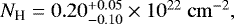 in good agreement with other values found in the literature, for example by Nordon et al. (2009) and Yu et al. (2009).
 -
Heat conduction imposes a temperature profile inside wind-blown bubbles that is able to provide consistence between temperature-sensitive line ratios of elements that reside preferentially in different parts of the bubble. Thus, a single bubble model is able to reproduce simultaneously the line ratios O VIII/O VII and Ne X/Ne IX. The characteristic X-ray temperature TX = 1.8 MK is lower than the 2.3 MK based on a one-temperature plasma model of Yu et al. (2009), but within the errors equal to the low-temperature value of their two-component model, 1.7 MK.
-
The use of our WR abundance set that is based on the analysis of the stellar spectrum of BD +30 by Marcolino et al. (2007; nearly identical with the work of Leuenhagen et al. 1996) yields line ratios for C/O and Ne/O consistent with the observations provided the neon abundance, not available from the stellar spectrum, is increased by a factor of about two. It is thus reasonable to conclude that the bubble of BD +30 has the same chemical composition as the star, with fractions of He, C, and O, as found by Marcolino et al. (2007) and of Ne from this work, and most likely no hydrogen at all (see Table 4).
-
Unfortunately, the abundance (relative to oxygen) of the important element nitrogen remains uncertain because of theweakness of the feature at 24.8 Å. We estimated an upper limit for nitrogen mass fraction that is considerably higher then assumed in our WR composition. The estimates of Nordon et al. (2009) and Yu et al. (2009) provide a similar value for N/O. However, their error margins are consistent with theassumption of no nitrogen at all.
-
Also, the abundances (relative to oxygen) for Mg, Si, and Fe could not be determined because of the weakness and uncertainty of the corresponding lines. In the case of Mg, we showed explicitly that the measurements must be systematically wrong, most likely due to severe blending.
-
Finding a subsolar number ratio of an element with respect to oxygen does not necessarily mean that the abundance of this particular element is subsolar. Rather, the low element-to-oxygen ratio can be the consequence of an increase of the oxygen abundance by helium burning while the element in question remains unchanged by nuclear processing.
-
Although our analysis of BD +30’s X-ray spectrum is fully consistent with the assumption of a purely hydrogen-free bubble with WR composition (with increased Ne content), a small contamination by hydrogen-rich matter cannot fully be excluded. At possibly lower hydrogen column densities as preferred here, the models predict C VI lines stronger than observed. However, only a very small amount of hydrogen-rich PN matter, not exceeding a 3% fraction of the bubble’s mass for the (unrealistic) NH = 0.10 case, suffices to reach agreement with the observed C VI/O VIII line ratio.
-
Even with such a maximally possible amount of hydrogen-rich matter contained in the bubble of BD+30, its X-ray emission is still dominated by the hydrogen-poor and carbon- and oxygen-rich matter provided by the shocked stellar wind. No substantial mixing between bubble and nebular matter and/or evaporation of nebular matter has obviously occurred so far. Despite this, the observed characteristic temperature of the emitting plasma is a factor of ten lower than predicted for an adiabatic shock – 1.8 versus 17 MK – and the only mechanism left for reducing the plasma temperature is thermal conduction across the bubble. This, of course, would then exclude the existence of a magnetic field.
-
The youth of the object (≲1000 yr) together with the practical absence of evaporated and/or mixed nebular matter contamination of the bubble suggests a scenario in which the separation between the hydrogen-rich nebula and the nuclearly processed hydrogen-poor interior regions must have occurred quite recently, namely, when the object was still at or close to the tip of the AGB.
Our models of hot bubbles would be very useful for (re)analyses of existing X-ray spectra of low spectral resolution, especially for the chemically homogeneous bubbles around normal central stars. It is straightforward to degrade the spectral resolution numerically and to apply extinction appropriate to the relevant hydrogen column density. This kind of model would provide a more physically consistent diagnostic tool than the single-temperature plasma models used to date.
Acknowledgements
The counsel of S. A. Zhekov helped us to reconstruct the mathematical framework of this study. R.H. received funding from the Deutsche Forschungsgemeinschaft (SCHO 394/29-1) and from the German Space Agency (Deutsches Zentrum für Luft- und Raumfahrt) under PLATO Data Center grant 50OO1501. This work has made use of NASA’s Astrophysics Data System Bibliographic Services. CHIANTI is a collaborative project involving George Mason University, the University of Michigan (USA), and the University of Cambridge (UK). We appreciate the anonymous referee’s very careful reading of the manuscript and her or his comments which helped considerably to improve the presentation of this work.
Appendix A Ionisation fractions
Figure A.1 displays the ionisation fractions of selected elements as a function of temperature as predicted by the Chianti software used by us. At temperatures above roughly 106 K which typically occur in hot bubbles, C V, C VI, N VI, N VII, O VII, O VIII, Ne IX, Ne X, Mg XI, and Mg XII emission lines are important for the diagnostics.
 |
Fig. A.1 Ionisation fractions of carbon (upper left panel), nitrogen (upper middle panel), oxygen (upper right panel), neon (lower left panel), magnesium (lower middle panel), and silicon (lower right panel) as a function of temperature (from CHIANTI’s default collisional ionisation equilibria tables “chianti.ioneq”). For each element, the sum of all ionisation fractions at a given temperature equals one. |
References
- Allen, C. W. 1976, Astrophysical Quantities (New York: Springer) [Google Scholar]
- Anders, E., & Grevesse, N. 1989, Geochim. Cosmochim. Acta, 53, 197 [Google Scholar]
- Arnaud, K., Borkowski, K. J., & Harrington, P. 1996, ApJ, 462, L75 [NASA ADS] [CrossRef] [Google Scholar]
- Blöcker, T. 1995, A&A, 299, 755 [NASA ADS] [Google Scholar]
- Borkowski, K. J., Balbus, S. A., & Fristrom, C. C. 1990, ApJ, 355, 501 [NASA ADS] [CrossRef] [Google Scholar]
- Bryce, M., & Mellema, G. 1999, MNRAS, 309, 731 [NASA ADS] [CrossRef] [Google Scholar]
- Campbell, W. W. 1893, PASP, 5, 204 [NASA ADS] [CrossRef] [Google Scholar]
- Castor, J., Mc Cray, R., & Weaver, R. 1975, ApJ, 200, L107 [NASA ADS] [CrossRef] [Google Scholar]
- Chu, Y.-H., Guerrero, M. A., Gruendl, R. A., Williams, R. M., & Kaler, J. B. 2001, ApJ, 553, L69 [NASA ADS] [CrossRef] [Google Scholar]
- Cowie, L. L., & McKee, C. F. 1977, ApJ, 211, 135 [NASA ADS] [CrossRef] [Google Scholar]
- Crowther, P. A., Morris, P. W., & Smith, J. D. 2006, ApJ, 636, 1033 [NASA ADS] [CrossRef] [Google Scholar]
- Dere, K. P., Landi, E., Mason, H. E., Monsignori Fossi, B. C., & Young, P. R. 1997, A&AS, 125, 149 [NASA ADS] [CrossRef] [EDP Sciences] [Google Scholar]
- Dere, K. P., Landi, E., Young, P. R., et al. 2009, A&A, 498, 915 [NASA ADS] [CrossRef] [EDP Sciences] [Google Scholar]
- Freeman, M. J., & Kastner, J. H. 2016, ApJS, 226, 15 [NASA ADS] [CrossRef] [Google Scholar]
- Freeman, M. J., Montez, Jr. R., Kastner, J. H., et al. 2014, ApJ, 794, 99 [NASA ADS] [CrossRef] [Google Scholar]
- Girard, P., Köppen, J., & Acker, A. 2007, A&A, 463, 265 [NASA ADS] [CrossRef] [EDP Sciences] [Google Scholar]
- Gorenstein, P. 1975, ApJ, 198, 95 [NASA ADS] [CrossRef] [Google Scholar]
- Guerrero, M. A., Chu, Y.-H., Gruendl, R. A., Williams, R. M., & Kaler, J. B. 2001, ApJ, 553, L55 [NASA ADS] [CrossRef] [Google Scholar]
- Guerrero, M. A., Gruendl, R. A., & Chu, Y.-H. 2002, A&A, 387, L1 [NASA ADS] [CrossRef] [EDP Sciences] [Google Scholar]
- Guerrero, M. A., Ruiz, N., Hamann, W.-R., et al. 2012, ApJ, 755, 129 [NASA ADS] [CrossRef] [Google Scholar]
- Hanami, H., & Sakashita, S. 1987, A&A, 181, 343 [NASA ADS] [Google Scholar]
- Kahn, F. D., & Breitschwerdt, D. 1990, MNRAS, 242, 505 [NASA ADS] [CrossRef] [Google Scholar]
- Karakas, A. I. 2003, Ph.D. Thesis, Monash University, Australia [Google Scholar]
- Kastner, J. H., Soker, N., Vrtilek, S. D., & Dgani, R. 2000, ApJ, 545, L57 [NASA ADS] [CrossRef] [Google Scholar]
- Kastner, J. H., Li, J., Vrtilek, S. D., et al. 2002, ApJ, 581, 1225 [NASA ADS] [CrossRef] [Google Scholar]
- Kastner, J. H., Montez, Jr. R., Balick, B., & De Marco O. 2008, ApJ, 672, 957 [NASA ADS] [CrossRef] [Google Scholar]
- Kastner, J. H., Montez, Jr. R., Balick, B., et al. 2012, AJ, 144, 58 [NASA ADS] [CrossRef] [EDP Sciences] [Google Scholar]
- Keller, G. R., Bianchi, L., & Maciel, W. J. 2014, MNRAS, 442, 1379 [NASA ADS] [CrossRef] [Google Scholar]
- Kingsburgh, R. L., & Barlow, M. J. 1994, MNRAS, 271, 257 [NASA ADS] [CrossRef] [Google Scholar]
- Kreysing, H. C., Diesch, C., Zweigle, J., et al. 1992, A&A, 264, 623 [NASA ADS] [Google Scholar]
- Leuenhagen, U., & Hamann, W.-R. 1998, A&A, 330, 265 [NASA ADS] [Google Scholar]
- Leuenhagen, U., Hamann, W.-R., & Jefferey, C. S. 1996, A&A, 312, 167 [NASA ADS] [Google Scholar]
- Li, J., Harrington, J. P., & Borkowski, K. J. 2002, AJ, 123, 2676 [NASA ADS] [CrossRef] [Google Scholar]
- Lodders, K. 2010, in Principles and Perspectives in Cosmochemistry, Astrophys. Space Sci. Proc. (Berlin: Springer), 16, 379 [NASA ADS] [CrossRef] [Google Scholar]
- Marcolino, W. L. F., Hillier, D. J., de Araujo, F. X., & Pereira, C. B. 2007, ApJ, 654, 1068 [NASA ADS] [CrossRef] [Google Scholar]
- Mellema, G., & Lundqvist, P. 2002, A&A, 394, 901 [NASA ADS] [CrossRef] [EDP Sciences] [Google Scholar]
- Montez, Jr. R., & Kastner, J. H. 2013, ApJ, 766, 26 [NASA ADS] [CrossRef] [Google Scholar]
- Montez, Jr. R., De Marco, O., Kastner, J. H., & Chu, Y.-H. 2010, ApJ, 721, 1820 [NASA ADS] [CrossRef] [Google Scholar]
- Montez, Jr. R., Kastner, J. H., Balick, B., et al. 2015, ApJ, 800, 8 [NASA ADS] [CrossRef] [Google Scholar]
- Morrison, R., & McCammon, D. 1983, ApJ, 270, 119 [NASA ADS] [CrossRef] [Google Scholar]
- Murashima, M., Kokubun, K., Makishima, K, et al. 2006, ApJ, 647, L131 [NASA ADS] [CrossRef] [Google Scholar]
- Nordon, R., Behar, E., Soker, N., Kastner, J. H., & Yu, Y. S. 2009, ApJ, 695, 834 [NASA ADS] [CrossRef] [Google Scholar]
- Pauldrach, A., Puls, J., Kudritzki, R.-P., Méndez, R. H., & Heap, S. R. 1988, A&A, 207, 123 [NASA ADS] [Google Scholar]
- Perinotto, M., Schönberner, D., Steffen, M., & Calonaci, C. 2004, A&A, 414, 993 [NASA ADS] [CrossRef] [EDP Sciences] [Google Scholar]
- Pittard, J. M., Dyson, J. E., & Hartquist, T. W. 2001a, A&A, 367, 1000 [NASA ADS] [CrossRef] [EDP Sciences] [Google Scholar]
- Pittard, J. M., Hartquist, T. W., & Dyson, J. E. 2001b, A&A, 373, 1043 [NASA ADS] [CrossRef] [EDP Sciences] [Google Scholar]
- Pottasch, S. R., & Bernard-Salas, J. 2006, A&A, 457, 189 [NASA ADS] [CrossRef] [EDP Sciences] [Google Scholar]
- Ruiz, N., Guerrero, M. A., Chu, Y.-H., & Gruendl, R. A. 2011, AJ, 142, 91 [NASA ADS] [CrossRef] [Google Scholar]
- Ruiz, N., Chu,Y.-H., Gruendl, R. A., et al.. 2013, ApJ, 767, 35 [NASA ADS] [CrossRef] [Google Scholar]
- Sandin, C., Steffen, M., Jacob, R., et al. 2012, in Planetary Nebulae: An Eye to the Future, eds. A. Manchado, L. Stanghellini, & D. Schönberner, IAU Symp. 283, 494 [NASA ADS] [Google Scholar]
- Sandin, C., Steffen, M., Schönberner, D., & Rühling, U. 2016, A&A, 586, A57 (Paper I) [NASA ADS] [CrossRef] [EDP Sciences] [Google Scholar]
- Schönberner, D., Jacob, R., Steffen, M., et al.. 2005, A&A, 431, 963 [NASA ADS] [CrossRef] [EDP Sciences] [Google Scholar]
- Schönberner, D., Jacob, R., Lehmann, H., et al.. 2014, Astron. Nachr., 335, 378 [NASA ADS] [CrossRef] [Google Scholar]
- Schönberner, D., Jacob, R., Heller, R., & Steffen, M. 2017, in Planetary Nebulae: Multi-wavelength Probes of Stellar and Galactic Evolution, eds. X. Liu, L. Stanghellini, & A. Karakas, IAU Symp. 323, 109 [NASA ADS] [Google Scholar]
- Spitzer, L. 1962, Physics of Fully Ionized Gases, 2nd edn. (New York: John Wiley & Sons, Inc.) [Google Scholar]
- Steffen, M., Schönberner, D., & Warmuth, A. 2008, A&A, 489, 173 [NASA ADS] [CrossRef] [EDP Sciences] [Google Scholar]
- Steffen, M., Sandin, C., Jacob, R., & Schönberner, D. 2012, in Planetary Nebulae: An Eye to the Future, eds. A. Manchado, L. Stanghellini, & D. Schönberner, IAU Symp. 283, 215 [NASA ADS] [Google Scholar]
- Stute, M., & Sahai, R. 2006, ApJ, 651, 882 [NASA ADS] [CrossRef] [Google Scholar]
- Toalá, J. A., & Arthur, S. J. 2014, MNRAS, 443, 3486 [NASA ADS] [CrossRef] [Google Scholar]
- Toalá, J. A., & Arthur, S. J. 2016a, MNRAS, 463, 4438 [NASA ADS] [CrossRef] [Google Scholar]
- Toalá, J. A., & Arthur, S. J. 2016b, MNRAS, 464, 178 [NASA ADS] [CrossRef] [Google Scholar]
- Todt, H., & Hamann, W.-R. 2015, in Wolf-Rayet Stars, Proceedings of an International Workshop, eds. W.-R. Hamann, A. Sander & H. Todt (Potsdam: Universitätsverlag), 253 [Google Scholar]
- Villaver, E., Manchado, A., & García-Segura, G. 2020, ApJ, 581, 1204 [Google Scholar]
- Weaver, R., McCray, R., Castor, J., Shapiro, P., & Moore, R. 1977, ApJ, 218, 377 [NASA ADS] [CrossRef] [Google Scholar]
- Yu, Y. S., Nordon, R., Kastner, J. H., et al. 2009, ApJ, 690, 440 [NASA ADS] [CrossRef] [Google Scholar]
- Zhekov, S. A., & Perinotto, M. 1996, A&A, 309, 648 (ZP96) [NASA ADS] [Google Scholar]
- Zhekov, S. A., & Perinotto, M. 1998, A&A, 334, 239 [NASA ADS] [Google Scholar]
This condition means that the radius of the conduction front we are interested in is about equal to the swept-up shell (i.e. of the rim). The slow wind characterises the flow of matter ahead of the rim, which is here the ionised shell of the planetary nebula where usually most of the nebular matter resides and which is driven by thermal pressure caused by ionisation heating.
The conduction constant C is defined via the coefficient D of the heat equation q = D ∇Te,
 , where q is the heat flux and Te the electron temperature. Following Paper I, Figs. 2 and 8 therein, it turns out that, for a (pure) hydrogen plasma, C = 6.0 × 10⁻⁷ erg cm−1 s−1 K−7∕2, for ln Λ = 30. This is in contrast to the value 1.2 × 10⁻⁶ erg cm−1 s−1 K−7∕2 given by Castor et al. (1975) and which is predominantly but erroneously used in the literature (but see also Borkowski et al. 1990 who used the value given here). The difference is obviously due to the neglect of the factor ϵ (=0.42) which has been recommended by Spitzer (1962); see also Cowie & McKee (1977). The effective charge Z of the WR composition used here (cf. Table 2) is about 4 for the case of full ionisation, hence the conduction efficiency is reduced by a factor of about two (see Table 1 in Paper I), and C = 3 × 10⁻⁷ erg cm−1 s−1 K−7∕2 follows for the WR plasma.
We note that the “kinematical age” as used in the literature is actually the present timescale of evolution and may not represent the “true” post-AGB age. A thorough discussion of various definitions of kinematical timescales is given in Schönberner et al. (2014).
We kept a finite hydrogen content because the evolutionary history of BD +30 is not known a priori. Anyway, the small amount used by us is also compatible with the assumption of no hydrogen at all.
Since the beginning of our work, new versions of the CHIANTI software package have appeared, the latest beeing v8. We compared the relevant ionisation fractions generated by the actual CHIANTI version with the corresponding fractions used throughout the paper and could not find significant differences in the temperature range of interest.
The CHIANTI manual says: “Lines marked with an * do not have correspondent observed energy levels and have approximate wavelengths.”
The X-ray bubble is younger than the nebula because of the aforementioned time delay of bubble formation due to line cooling.
The value of RB = 0.023 pc = 7 × 1016 cm (distance = 1200 pc) given in Table 1 of Kastner et al. (2008) is actually the diameter.
As an example, 40 × 10−6 cm−2 s−1 photons detected at 18.966 Å from O VIII and 38.2 × 10⁻⁶ cm−2 s−1 photons observed at 21.607 Å for the O VII line (Yu et al. 2009) translate into a line ratio of  in terms of energy units, instead of 1.047.
Since Yu et al. (2009) used the Anders & Grevesse (1989) solar oxygen abundance ϵ = 8.93, their Ne/O value relative to the solar one has been corrected for the new solar oxygen abundance of ϵ = 8.73 (Lodders 2010).
The only exceptions are the works of Yu et al. (2009) and Nordon et al. (2009) in which a two-temperature plasma model was applied to get an overall better spectral fit compared to a single-temperature plasma.
The Toalá & Arthur (2016a) bubbles cannot be used for comparison with BD +30 because they are hydrogen-rich. As we show in our Figs. 2 and 15, bubbles with WR composition are much more luminous than their hydrogen rich counterparts (see also Steffen et al. 2012).
All Tables
Chemical compositions of the stellar photosphere and wind (WR) and the nebular gas (PN) used in this work, arranged by order of atomic number Z as mass fractions (Cols. 3 and 5) and (logarithmic) number fractions (ϵ) relative to hydrogen (Cols. 4 and 6).
Parameters of the “best-fit” bubble model and observed values of BD +30° 3639’s hot bubble.
All Figures
|
Fig. 1 Variations of the quantities |
| In the text | |
|
Fig. 2 Examples of bubble structures (left panels) and X-ray emissions (middle and right panels) for hydrogen-rich (PN, top panels) and hydrogen-poor (WR, bottom panels) composition. The inner boundaries are at the position of the reverse wind shock (0.67 × 1016 cm), the outer boundaries at the (heat) conduction front at 1.54 × 1016 cm. The planetary nebula proper is on the right side of this front. Both HBs have a similar parameterisation: age = 500 yr, Ṁ sw = 10−5 M⊙ yr−1, vsw = 25 km s−1 , but C = 6 × 10⁻⁷(top panels) and C = 3 × 10⁻⁷ erg cm−1 s−1 K−7∕2 (bottom panels). The bubble structures are characterised by the radial runs of electron temperature (solid), total particle number density (long dashed), ion number density (dashed), and electron density (dotted). We note the linear scale for the temperature, but the logarithmic scale for the densities. The characteristic X-ray temperatures of the bubbles are 2.9 MK (PN) and 2.4 MK (WR), respectively. The intrinsic X-ray surface brightnesses of these two bubble models are displayed in the middle panels and correspond to the emission (spectral luminosity density) in wavelength bands of 5–40 Å (0.3– 2.5 keV) shown in the right panels. The positions of the respective wind reverse shocks (= inner bubble boundaries) are indicated by the arrows. The X-ray luminosities in the given wavelength band are 3.7 × 1032 erg s−1 (PN) and 1.5 × 1034 erg s−1 (WR). |
| In the text | |
|
Fig. 3 Radial distribution of ionic fractions of carbon (top panels), oxygen (middle panels), and neon (bottom panels) inside the two bubbles shown in Fig. 2. Left column: PN composition, right column: WR composition. |
| In the text | |
|
Fig. 4 Zoom-in on spectral windows of the CHIANTI output that were considered for our analyses. We note the logarithmic scale on the ordinate and the numerous contributing lines. Without loss of generality, the bubble used is that shown in the top panels of Fig. 2. The hydrogen-rich PN case has been chosen in order to highlight the N VII line, which is virtually absent for the WR composition. We show the spectra at different resolutions (see legend), the spectral range and resolution chosen for the line integration (red), the continuum (short-dashed), and the domains where the continuum is defined for the integrations (blue, on the abscissae). |
| In the text | |
|
Fig. 5 Dependence of the bubble properties in terms of the line ratio O VIII/O VII (18.97 Å/21.60 Å) versus TX on age (panel I), and slow-wind properties (panels II and III). The fixed model parameters are indicated at the top of the respective panels. In each of these three panels, we distinguish between three values of the conduction parameter C: 3.0 × 10⁻⁷ (grey), 4.5 × 10⁻⁷ (open), and 6.0 × 10⁻⁷ erg cm−1 s−1 K7∕2 (filled), as indicated in the legends. Top left panel: all computed bubble models, and the annotated areas (I, II, and III) indicate the plot ranges shown in the respective panels I, II, and III. Without any loss of generality, we selected the WR model shown in Fig. 2, which is close to the middle of the parameter space listed in Table 1, as the reference model. The bubbles’ chemical composition corresponds to the WR case of Table 2. |
| In the text | |
|
Fig. 6 Same as in the top left panel of Fig. 5 but now including also bubble models with hydrogen-rich PN-matter (symbols with black central line, C = 6.0 × 10⁻⁷ erg cm−1 s−1 K7∕2), and single-temperature bubbles (iso-HB, small triangles). |
| In the text | |
|
Fig. 7 X-ray luminosity (5–40 Å, 0.3–2.5 keV) versus bubble size for the bubble sub-grid with WR composition and C = 3 × 10⁻⁷ erg cm−2 s−1 K−7∕2, and for ages from 200 to 1000 yr. Black dots indicate individual bubble models. The slow wind, Ṁ sw , ranges from 10−7 to 10−4 M⊙ yr−1, the slow-wind velocity, V sw, from 10 to 40 km s−1 (cf. Table 1). The adopted values for BD +30 (see text) are marked by the filled star. The open stars indicate the positions if the assumed distance to BD +30 is increased or decreased by a factor of two. |
| In the text | |
|
Fig. 8 Line ratio of O VIII/O VII over line ratio Ne X/Ne IX for BD +30 (error cross) after Yu et al. (2009, Table 2) and for ZP96 heat-conducting bubbles with homogeneous hydrogen-poor WR composition subject to various absorptions as indicated in the legend. Individual models are only shown for NH = 0 (circles) and NH = 0.20 × 1022 cm−2, the value adopted (grey dots). For other values of NH, only envelopes are given in order to avoid confusion. Evolution proceeds from low to high line ratios, that is, from low to high TX. The oldest (1000 yr) and hottest (4 MK) bubble models always have neon line ratios of about 2, virtually independent of NH. The crosses are the models that lie within BD +30’s error box. The filled square (green) marks our “best-fit” bubble model, presented in Sect. 4.3. The filled triangles are bubbles with constant temperatures (iso-HB, for NH = 0.20 × 1022 cm−2 only, see text for details). The numbers along the iso-HB sequence indicate the bubble temperatures in MK. |
| In the text | |
|
Fig. 9 Sameas in Fig. 8 but now for O VIII/O VII over Mg XII/Mg XI (left panel) and over C VI/C V (right panel), and only for NH = 0.20 × 1022 cm−2. The symbols have the same meaning as in Fig. 8. The position of the “best-fit” models is either the filled (green, rightpanel) or crossed square (left panel). |
| In the text | |
|
Fig. 10 Absorbed line ratios of Mg XII/O VIII over Mg XI/O VIII (left panel) and Ne X/O VIII over Ne IX/O VIII for NH = 0.20 × 1022 cm−2 and the resp- ective observed line ratios for BD +30 (error cross). The symbols have the same meaning as in Fig. 8 (or Fig. 9). The parallel lines indicate the shift of the crossed models (and the “best-fit” model as well) if the original bubble abundances of Mg (left panel) or Ne (right panel) are multiplied by the given factor. The corresponding shifts of the remaining bubble models are not shown in order to avoid confusion. |
| In the text | |
|
Fig. 11 Same as in Fig. 8 but for Si XIII/O VIII over Ne X/O VIII and for NH = 0.20 × 1022 cm−2. The grey dots and crosses mark the sequence of our ZP96 bubbles with the new, enhanced neon abundance; the crossed square indicates the “best-fit” model. |
| In the text | |
|
Fig. 12 Same as in Fig. 8 but for O VIII/C VI over Ne X/C VI and for NH = 0.20 × 1022 cm−2. The neon abundance from Table 2 (WR) is increased by a factor of two. The horizontal shift of the bubbles from their original positions is indicated by the error in the upper left corner of the plot. The green square marks our “best-fit” bubble (see text). Filled triangles represent our iso-HB models, also shifted accordingly. |
| In the text | |
|
Fig. 13 Upper limit of the observed line ratio N VII/O VIII versus Ne X/Ne IX compared to the model prediction. Symbols have the same meaning as in the previous figures. |
| In the text | |
|
Fig. 14 Physical structure of a ZP96 bubble of age = 500 yr with a stratified composition such that ω ≡ MPN∕(MWR + MPN) = 0.03, with MWR = 5.59 × 1028 g and MPN = 1.67 × 1027 g, and with C = 3 × 10⁻⁷ erg cm−1 s−1 K7∕2, Ṁ sw = 5.0 × 10⁻⁷ M⊙ yr−1, and vsw = 25 km s−1. Shown are radial runs of electron, ion, total particle densities, and temperature. The central star is at the origin (radius = 0 cm), the wind reverse shock (= inner bubble boundary) is at 2.97 × 1016 cm, and the planetary nebula proper adjacent to the heat conduction front at 4.18 × 1016 cm. The compositions are those listed in Table 2: WR for hydrogen-deficient (grey) and PN for hydrogen-rich. The chemical discontinuity is at 3.98 × 1016 cm, or 2.0 × 10⁶ K. We note the logarithmic ordinate scales and the linear abscissa. For the meaning of the dots along the abscissa, see Fig. 15. See also Sect. 5.1 for details. |
| In the text | |
|
Fig. 15 Intrinsic intensity distributions of X-ray emission between 5 and 40 Å for the bubble used in Fig. 14 but with the chemical discontinuity located at different bubble radii, hence with different ω. The individual intensity distributions correspond either to the specific bubble model of Fig. 14 (solid) or to the positions of the chemical discontinuities being at radii indicated by the filled circles in Fig. 14 (dotted), whereas the two chemically homogeneous cases PN and WR are rendered as dashed lines. The model belonging to the open circle in Fig. 14 is not shown because of its similarity to the ω = 0.03 model. The numbers at the curves indicate the X-ray luminosities (in 1032 erg s−1 ) computed for the given wavelength range. |
| In the text | |
|
Fig. 16 X-ray spectral luminosity (left panels) and selected lines zoomed-in (right panels) of ZP96 bubbles with homogeneous WR composition (ω = 0.00, solid/black) and inhomogeneous WR + PN composition (ω = 0.03, dashed/red, and 0.15, dotted/blue). All three bubble models have the same dimension and temperature profile, and the one used in the middle-left panel is the model used in Figs. 14 and 15. The line-profile panels (grey) cover the wavelength range of 0.10 Å each (i.e. the Chandra resolution), but the (logarithmic) ordinate range may be diffferent so as to give a better match to the various line strengths. Also, all lines are normalised to a single continuum level to ease comparison. |
| In the text | |
|
Fig. 17 Characteristic X-ray temperature TX (top panel) and X-ray luminosity LX (bottom panel) for a suite of chemically stratified heat-conduction bubbles constructed from pure WR ZP96 models that comply with both the observed oxygen and neon line ratios of BD +30 (crosses in Fig. 8) versus ω = MPN∕(MPN + MWR). The thick line corresponds to the model sequence originating from the 500-yr old “best-fit” WR-model. We note the break of the abscissa scale at ω = 0.05. The wavelength range considered is 5–40 Å (0.3–2.5 keV.) |
| In the text | |
|
Fig. 18 Same as in Fig. 12 but for bubble models with lower absorptions as indicated in the respective panels. Filled circles give the positions of the bubbles with homogeneous WR composition (ω = 0 ) that comply with the constraints from Fig. 8 with the appropriate NH value. The green lines enclose the corresponding positions if in the outer bubble parts the WR mixture is replaced by PN mixture (ω = 0.03, left panel, and ω = 0.02, right panel). |
| In the text | |
|
Fig. A.1 Ionisation fractions of carbon (upper left panel), nitrogen (upper middle panel), oxygen (upper right panel), neon (lower left panel), magnesium (lower middle panel), and silicon (lower right panel) as a function of temperature (from CHIANTI’s default collisional ionisation equilibria tables “chianti.ioneq”). For each element, the sum of all ionisation fractions at a given temperature equals one. |
| In the text | |
Current usage metrics show cumulative count of Article Views (full-text article views including HTML views, PDF and ePub downloads, according to the available data) and Abstracts Views on Vision4Press platform.
Data correspond to usage on the plateform after 2015. The current usage metrics is available 48-96 hours after online publication and is updated daily on week days.
Initial download of the metrics may take a while.