| Issue |
A&A
Volume 684, April 2024
|
|
|---|---|---|
| Article Number | A105 | |
| Number of page(s) | 25 | |
| Section | Interstellar and circumstellar matter | |
| DOI | https://doi.org/10.1051/0004-6361/202346170 | |
| Published online | 09 April 2024 | |
Hot bubbles of planetary nebulae with hydrogen-deficient winds
III. Formation and evolution in comparison with hydrogen-rich bubbles★
Leibniz-Institut für Astrophysik Potsdam,
An der Sternwarte 16,
14482
Potsdam,
Germany
e-mail: This email address is being protected from spambots. You need JavaScript enabled to view it.
; This email address is being protected from spambots. You need JavaScript enabled to view it.
Received:
17
February
2023
Accepted:
20
December
2023
Abstract
Aims. We seek to understand the evolution of Wolf–Rayet central stars by comparing the diffuse X-ray emission from their windblown bubbles with that from their hydrogen-rich counterparts with predictions from hydrodynamical models.
Methods. We simulate the dynamical evolution of heat-conducting wind-blown bubbles using our 1D radiation-hydrodynamics code NEBEL/CORONA. We use a post-AGB-model of 0.595 M⊙ but allow for variations of its evolutionary timescale and wind power. We follow the evolution of the circumstellar structures for different post-AGB wind prescriptions: for O-type central stars and for Wolf–Rayet central stars where the wind is hydrogen-poor, more dense, and slower. We use the CHIANTI software to compute the X-ray properties of bubble models along the evolutionary paths. We explicitly allow for non-equilibrium ionisation of key chemical elements. A sample of 12 planetary nebulae with diffuse X-ray emission – seven harbouring an O-type and five a Wolf–Rayet nucleus – is used to test the bubble models.
Results. The properties of most hydrogen-rich bubbles (X-ray temperature, X-ray luminosity, size) and their central stars (photon and wind luminosity) are fairly well represented by bubble models of our 0.595 M⊙ AGB remnant. The bubble evolution of Wolf–Rayet objects is different, thanks to the high radiation cooling of their carbon- and oxygen-rich winds. The bubble formation is delayed, and the early evolution is dominated by condensation instead of evaporation. Eventually, evaporation begins and leads to chemically stratified bubbles. The bubbles of the youngest Wolf–Rayet objects appear chemically uniform, and their X-ray properties can be explained by faster-evolving nuclei. The bubbles of the evolved Wolf–Rayet objects have excessively low characteristic temperatures that cannot be explained by our modelling.
Conclusions. The formation of nebulae with O-type nuclei follows mainly a single path, but the formation pathways leading to the Wolf–Rayet-type objects appear diverse. Bubbles with a pure Wolf–Rayet composition can exist for some time after their formation despite the presence of heat conduction.
Key words: conduction / hydrodynamics / stars: AGB and post-AGB / planetary nebulae: general / X-rays: stars
This work has made use of data from the European Space Agency (ESA) mission Gaίa (https://www.cosmos.esa.int/gaia), processed by the Gaίa Data Processing and Analysis Consortium (DPAC, https://www.cosmos.esa.int/web/gaia/dpac/consortium). Funding for the DPAC has been provided by national institutions, in particular the institutions participating in the Gaίa Multilateral Agreement.
© The Authors 2024
 Open Access article, published by EDP Sciences, under the terms of the Creative Commons Attribution License (https://creativecommons.org/licenses/by/4.0), which permits unrestricted use, distribution, and reproduction in any medium, provided the original work is properly cited.
This article is published in open access under the Subscribe to Open model. This email address is being protected from spambots. You need JavaScript enabled to view it. to support open access publication.
1 Introduction
By means of space-based observations, it became evident that the inner ‘cavities’ of many round or elliptical planetary nebulae are filled up with a tenuous but very hot gas that emits preferentially in the soft X-ray domain. The existence of such gas is to be expected: the fast central-star wind collides with the slower, denser inner parts of the nebula (the former wind envelope produced during the star’s previous evolution along the asymptotic giant branch (AGB)) and becomes shock-heated, producing a ‘bubble’ of very hot gas. Given the typical values of density and velocity of the stellar wind, the wind shock is adia-batic, and the shocked gas is expected to reach temperatures of 107 K (= 10 MK) or more.
However, all spectral analyses of the X-ray emissions reveal an unexpectedly low mean or characteristic X-ray temperature of between about 1 MK and a few MK. Also, the emission measure is much higher than expected. The present status and preliminary results of the extensive Chandra Planetary Nebula Survey (ChanPlaNS) can be found in Kastner et al. (2012) and Freeman et al. (2014).
Steffen et al. (2008, hereafter SSW) took up a suggestion by Soker (1994) that heat conduction across the hot bubble from the wind shock towards the bubble-nebula interface may be responsible for the unexpected bubble properties. Indeed, SSW were able to show that, although the dynamics of a model nebula remains virtually unchanged, the bubble structure and its characteristic properties, such as X-ray characteristic temperature and luminosity, can well be explained by nebula models that include thermal conduction. Further detailed comparisons between the SSW models and observations are given in Ruiz et al. (2013).
Another important physical process to reduce the temperature and to increase the density of the X-ray-emitting plasma of wind-blown bubbles of planetary nebulae is mixing between the hot bubble and cooler nebular gas across the bubble-nebula interface by Rayleigh-Taylor instabilities. The first ‘pilot’ 2D simulations of Stute & Sahai (2006) cover, however, only a very limited time span (≲300 yr) and have only simple param-eterised boundary conditions. They are thus not really suitable for drawing conclusions concerning the extent of mixing and the temporal evolution of the mixing efficiency.
More realistic 2D simulations have been presented by Toalá & Arthur (2014, 2016, 2017)1. These are based on the post-AGB evolutionary tracks of Vassiliadis & Wood (1994) and appropriate wind models in a similar manner to the simulations by Villaver et al. (2002) and Perinotto et al. (2004), and clearly show that mixing of bubble and nebular matter across the bubble-nebula interface generates a region with intermediate temperatures (≳ 1 MK) and sufficiently high densities for emitting X-rays of the observed properties. However, inclusion of heat conduction increases the amount of cooler matter by evaporation of nebular gas at the conduction front to such an extent that the effect of evaporation soon dominates over mixing.
It is well known that a small fraction of planetary nebulae harbour nuclei with hydrogen-poor but helium- and carbon-enriched surfaces (Wolf–Rayet central stars), which means they also have winds of the same composition that are feeding their hot bubbles. However, the formation and evolution of hydrogen-poor central stars is still not fully understood, and the existing post-AGB evolutionary models are not applicable, in principle.
Several important questions have to be addressed in this context. (1) It is presently unknown at which moment of the post-AGB evolution the originally hydrogen-rich stellar wind turns into a hydrogen-poor wind with the typical Wolf–Rayet composition. (2) One would like to understand how the formation and evolution of hydrogen-poor but carbon- and oxygen-rich bubbles is influenced by their high radiation cooling, and (3) how important chemical mixing by dynamical instabilities is in comparison to evaporation by heat conduction. (4) Finally, it is not clear to what degree evaporation and mixing of hydrogen-rich matter into the hydrogen-poor bubble, as predicted by the numerical models, actually occur in nature. At present, observational evidence for the existence of chemically stratified bubbles is still lacking.
Answering these open questions is certainly a very ambitious task. A detailed modelling of chemically inhomogeneous stellar-nebular systems in combination with appropriate observations will be essential to gain a better understanding of the formation and evolution of hydrogen-poor central stars.
In the first paper of this series (Sandin et al. 2016, henceforth Paper I), an algorithm for computing heat conduction coefficients for arbitrary chemical compositions was developed and tested. It was found that due to the high radiation cooling of hydrogen-poor but carbon- and oxygen-rich matter, the formation of a wind-blown bubble with heat conduction is considerably delayed.
In a second paper, Heller et al. (2018, henceforth Paper II) constructed analytical solutions for self-similar hot bubbles, which include thermal conduction according to the prescription of Zhekov & Perinotto (1996) but are modified to our needs. These simple models provide a convenient tool for analysing, for example, the high-resolution X-ray spectrum of the hot bubble around BD +30º3639. It could be shown that this particularly young and small bubble is fed by the hydrogen-poor and carbon/oxygen-rich stellar wind and most likely does not yet contain evaporated (and/or mixed) hydrogen-rich matter.
In the present paper, we report a parameter study addressing some of the questions outlined above. To this end, we constructed a set of hydrodynamical sequences consisting of chemically inhomogeneous stellar-nebular systems appropriate for comparison with existing X-ray observations of planetary nebulae with Wolf–Rayet central stars. This set is discussed in comparison with hydrodynamical sequences of chemically homogeneous, hydrogen-rich models already presented and discussed in SSW and Ruiz et al. (2013).
The structure of this paper is as follows: We start in Sect. 2 by providing the details of the new 1D radiation-hydrodynamics calculations with hydrogen-poor post-AGB winds, including a description of the assumptions made. Section 3 continues with a parameter study of hydrogen-poor wind-blown heat-conducting bubble models and a discussion of the related findings. Section 4 presents a compilation of the observed properties of seven O- and five Wolf–Rayet-type central stars and their windblown bubbles for which diffuse X-ray emissions have been observed. These observed properties are compared with the predictions of existing (hydrogen-rich) evolutionary simulations in Sect. 5, while Sect. 6 deals with a careful comparison of the properties of our newly computed chemically inhomogeneous models with the observed properties of the bubbles around Wolf–Rayet central stars. The results are discussed in Sect. 7, and we end the paper by providing a summary and our conclusions (Sect. 8).
The paper is supplemented by two Appendices, one describing how bubble temperature and luminosity depend on the chosen X-ray band width (Appendix A), and the other establishing the relations between the post-AGB evolutionary tracks used in this paper and the more recent ones of Miller Bertolami & Althaus (2006) (Appendix B).
2 Details of the model calculations
In this section we present a brief overview of our new hydro-dynamical simulations of hydrogen-poor, wind-blown heat-conducting bubbles inside planetary nebulae and the computations of the bubbles’ X-ray emission in terms of X-ray luminosity and characteristic (or mean) X-ray temperature.
2.1 General aspects
We used, as in previous works, the Potsdam NEBEL/CORONA software package to model the combined evolution of central star and circumstellar envelope by radiation-hydrodynamical simulations in spherical geometry. The details of the NEBEL code can be found in Perinotto et al. (1998, 2004). Here we outline only the physical system: A typical model has a radial extent from 6 × 10¹⁴ to 3 × 1018 cm (0.0002 to 1.0 pc). Treated in a consistent way, the model contains the freely expanding central-star wind, the inner reverse shock, the hot bubble of shocked stellar wind gas, and the nebula proper which is separated from the bubble by a contact discontinuity (or heat conduction front) and from the surrounding asymptotic giant-branch (AGB) wind (halo) by an outer, leading shock. The simulations start at the tip of the AGB and are advanced well into the white-dwarf regime, thus covering the formation and complete evolution of a planetary nebula.
The CORONA code treats ionisation/recombination and heating/cooling time-dependently for the nine elements H, He, C, N, O, Ne, S, Cl, and Ar (cf. Table 1, elements in italics) with up to 12 ionisation stages. Altogether, non-equilibrium number densities of 76 ions are evaluated at each time step and at all grid points. The full computational details and atomic data implemented can be found in Marten & Szczerba (1997). Heat conduction is included as in SSW, but now the heat conduction formalism holds for arbitrary chemical composition (see Paper I). Of course, heat conduction is only effective within the hot bubble where the electron density is low and the electron temperature sufficiently high.
Given the radial temperature and density structure of the hot bubble, we applied the well documented CHIANTI code (v6.0.1, Dere et al. 1997, 2009) to compute, for selected positions along the evolutionary sequence, the emergent X-ray spectrum, the X-ray luminosity, LX, the ‘characteristic’ (or ‘mean’) X-ray temperature, TX, and the surface brightness (intensity) profile of the hot bubble model. For more details about these calculations, see SSW.
We note that this method is inconsistent because the CHIANTI code always assumes collisional ionisation equilibrium (CIE) while our hydrodynamical models treat ionisation time-dependently (non-equilibrium ionisation (NEI)) for the nine elements listed above. Given the low electron densities of the hot bubbles together with the temperature profile imposed by heat conduction, significant departures from the ionisation equilibrium can be expected (e.g. Liedahl 1999; Mewe 1999).
We touched this problem already in SSW (cf. Fig. 1 therein) but concluded that the departures from the CIE case are not very important, especially in the context of the low quality of the existing X-ray observations, the uncertainty of the distances, and the approximations used in the implementation of thermal conduction. The present study, however, mainly deals with bubbles of hydrogen-poor chemical compositions where the significance of NEI effects is unknown. Additionally, the distances are now well known thanks to Gala. We therefore decided to reconsider the NEI case in order to clarify its general importance for interpreting the X-ray emission of wind-blown bubbles.
To this end, we developed an interface which allows the CHIANTI code to use the individual NEI ionisation fractions provided by our NEBEL/CORONA code for the nine considered elements. The (standard) CIE was adopted for the remaining elements. Since the ions of C, N, O, and Ne are the most prominent emitters in the X-ray regime of interest here, we believe that this ‘hybrid’ method suffices to provide realistic results for comparisons with the observations.
As in Paper I, we allow for a chemical stratification of the model: The initial circumstellar envelope has always a normal hydrogen-rich composition (dubbed ‘PN’), while the central-star wind may be hydrogen-poor with an element mixture (dubbed ‘WR’) which is typical for the Wolf–Rayet central stars. The two sets of chemical abundances are listed in Table 1 in both the mass fractions normalised to unity and the number fractions normalised to the hydrogen abundance ϵH = 12.
The PN mixture is representative of the composition of many planetaries of the Galactic disk and has already been chosen for the hydrodynamical simulations of Perinotto et al. (2004). The WR composition is based on the Marcolino et al. (2007) analysis of BD +30º3639. All elements not accessible to observations were supplemented assuming solar mass fractions (see Table 1). Exceptions exist for nitrogen and neon. Since the WR composition represents the chemistry of the (somehow) exposed intershell region between the hydrogen- and helium-burning shell of the progenitor star, we assume that complete hydrogen burning first converts virtually all C and O nuclei into nitrogen, which is later converted into neon (22Ne) within the helium-burning shell. This scenario implies a very low nitrogen abundance (we adopt a mass fraction of 10−5) and justifies a very high neon abundance for the WR composition (1.4 × 10⁻² by mass) which exceeds considerably the original surface value that is mainly due to 20Ne. We note in this context that Marcolino et al. (2007) estimated a photospheric neon mass fraction of ≃2 % for BD +30º3639, consistent with the 1.4 % used here.
We emphasise that our WR element mixture is genuinely hydrogen-poor, with helium and carbon being the most abundant elements. This obviously is not the case in the study of Toalá & Arthur (2018) in which the authors used a chemical composition with hydrogen still being the most abundant element for the case of BD+30º3639.
Chemical composition of the stellar wind (WR) and the nebular gas (PN) used for computing the hydrodynamical models and synthetic X-ray spectra in terms of mass fractions (Cols. 3 and 5) and (logarithmic) number fractions ϵ (Cols. 4 and 6), arranged by atomic number Z.
2.2 The characteristic bubble temperature
Once the temperature and density profiles of a hot bubble are known, one can compute a characteristic (or mean) X-ray temperature
 (1)
(1)
of the bubble plasma. Here, Te(r) is the electron temperature between inner, R1, and outer radius, R2, of the bubble, and
 (2)
(2)
is the X-ray luminosity, with
 (3)
(3)
being the volume emissivity in the energy band E1 − E2 (cf. Steffen et al. 2008). While TX is an emission weighted mean temperature, the true temperature inside a hot bubble is a function of distance from the central star and is here ruled by heat conduction. It is therefore clear that identical temperature structures can result in different values of TX because the latter depend also on the emissivity distribution (cf. Eq. (1)), and therefore on the bubble’s chemical composition. A thorough investigation of how the X-ray emission of a bubble plasma depends on chemical composition, heat conduction efficiency, and boundary conditions can be found in Paper II on the basis of analytical bubble models.
Both the X-ray luminosity and characteristic temperature TX depend on the chosen energy window. The high-energy limit, 2 keV (6.2 Å), is of no problem since above this energy there is no or only very little emission for the observed bubble temperatures. This is different at the low-energy end, but there the detector sensitivity becomes low and the extinction high. We used throughout the paper the energy band 0.3–2.0 keV (6.2–41.3 Å) because it also has been used in Ruiz et al. (2013) to whose compilation of X-ray data we mostly refer (see Appendix A for an investigation of the influence of the chosen X-ray band width on luminosity and mean temperature).
SSW derived the following important relation for the mean temperature 〈T〉 of a heat-conducting bubble:
 (4)
(4)
where  is the wind power and R2 the bubble radius (for the details, see Eqs. (9) through (14) in SSW). In deriving Eq. (4) it has been assumed that (i) the bubble mass is dominated by evaporated matter, (ii) the bubble is chemically homogeneous, and (iii) the radiation losses are negligible. Of course, a similar kind of relation also must hold for the characteristic temperature TX as defined by Eq. (1).
Equation (4) shows that the mean temperature of a heat conducting bubble is not directly dependent on the wind velocity. Rather, the temperature depends exclusively on the actual ratio of stellar wind power to bubble size, independently of the bubble mass. Therefore, Eq. (4) predicts an evolution of TX while the central star crosses the Hertzsprung-Russell diagram (HRD), and which can easily be tested; see discussion in Sect. 5.3 in the context of Fig. 13).
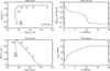 |
Fig. 1 Evolution of stellar parameters and wind properties of our standard model of a 0.595 M⊙ AGB remnant. Left column: Run of stellar bolometric, Lstar/L⊙ (top), and wind luminosity, |

2.3 Setup of the physical system consisting of a central star and an AGB wind envelope
A realistic modelling of the nebular structures (as done, e.g. in Perinotto et al. 2004), is not in the focus of the present work and not really necessary. In order to keep the number of model sequences as small as possible, we employ only a single post-AGB evolutionary model, viz. the 0.595 M⊙ model and combine it with always the same AGB envelope as initial outer boundary, both of which have already been used in SSW. However, here we vary the strength of the stellar wind, its chemical composition, and in some cases also the evolutionary speed across the HRD, in order to mimic various possible evolutionary scenarios. In this sense we treat wind power and evolutionary timescale as free and independent parameters. We emphasise that only the radiation field, the wind power, and the speed of the stellar evolution enter in the hydrodynamical simulations, but not the stellar mass.
Figure 1 renders the properties of the star-wind model used in this work in terms of stellar effective temperature and post-AGB time (our ‘reference simulation’). The relevant quantity for powering any X-ray emission is the mechanical luminosity of the stellar wind. According to the theory of radiation-driven winds for standard hydrogen-rich chemical composition in the formulation of Pauldrach et al. (1988), the mass-loss rate and the wind speed are coupled to the stellar parameters mass, luminosity, and effective temperature. Based on this wind prescription, the mechanical energy transported by the wind increases during the evolution across the HRD, simply because the slowly decreasing mass-loss rate is over-compensated by the increasing wind speed (Fig. 1, bottom right). However, when the hydrogen-burning shell becomes exhausted, the mass loss rate drops sharply in line with the stellar luminosity, causing also the mechanical wind power to drop considerably since the wind speed remains now virtually constant with a maximum value of about 10 000 km s−1.
Overall, the mechanical power remains rather small and does not exceed 1% of the stellar photon luminosity in this particular case (Fig. 1, left column). According to this wind model, the maximum of the mechanical power occurs close to maximum stellar temperature. Only very little of the stellar mass is carried away by the wind during the whole transition to the white-dwarf domain, viz. ≈3 × 10⁻⁴ M⊙, which is to be compared with the typical planetary nebula mass of a tenth of a solar mass.
We emphasise that most of this mass is already lost with low speed during the first 1000 yr of the transition to the planetary nebula stage. Only during this phase we have wind speeds as low as a few 100 km s−1, i.e. low enough to provide post-shock temperatures of the order of 106 K. These mass-loss parameters are typical for the ‘early’ wind and are here based on the Reimers (1975) prescriptions. The total stellar mass lost during the following nebula stage is only about 8 × 10⁻⁵ M⊙, but this material has a very high kinetic energy because of its large speed exceeding 1000 km s−1, leading to (adiabatic) post-shock temperatures well in excess of 107 K.
The evolutionary timescale of the 0.595 M⊙ model depicted in the upper left panel of Fig. 1 is fully consistent with the assumed wind (mass-loss) model; that is, the evolution is driven by envelope consumption due to both hydrogen-burning at the bottom of the envelope and mass loss from its surface (Schönberner & Blöcker 1993; Blöcker 1995) in a consistent way. Mass loss dominates in the vicinity of the AGB in driving the stellar evolution while later, when ionisation sets in, mass loss becomes unimportant and nuclear burning takes over.
To simulate the evolution of nebulae with a WR-type central star, we explicitly allow for different chemistries between the AGB envelope and the post-AGB wind. While the chemical composition of the envelope is kept hydrogen-rich (PN), the post-AGB wind is switched at t = 0 yr (cf. Fig. 1) to a hydrogen-poor composition (WR). With such an initial setup, we implicitly assume that the conversion from a hydrogen-rich to a hydrogen-poor AGB remnant occurs right at the end of the AGB evolution when the remnant begins to leave the tip of the AGB. The contact discontinuity (or the surface of the bubble) is initially also a chemical discontinuity which will move into the bubble when evaporation of the hydrogen-rich nebular matter occurs.
The assumption of keeping a hydrogen-rich nebular composition is justified by the absence of any evidence that the nebulae around [WR] central stars, or parts of them, have hydrogen-poor compositions (see, e.g. Górny & Stasińska 1995; Girard et al. 2007).
It is also possible that the switch of the stellar surface from hydrogen-rich to hydrogen-poor occurs at a later point during the crossing of the HRD. Observationally, [WR]-type nuclei show already up as rather cool objects (Teff ≈ 20 000 K, Hamann 1997) around very young planetary nebulae. The formation of these central stars must have occurred at or at least close to the tip of the AGB. Nevertheless, we set up a test simulation for which the switch from a hydrogen-rich to a hydrogen-poor wind occurred 1000 yr after departure from the AGB (corresponding Teff ≃ 10 000 K in Fig. 1). It turns out that the resulting bubble structures differ only slightly from the case where this switch occurs immediately at the tip of the AGB. Our choice of t = 0 yr as the starting point for the hydrogen-deficient wind therefore appears to be a reasonable assumption.
3 Parameter study of the formation and evolution of hydrogen-deficient hot bubbles
In this section, we present and discuss our bubble simulations where a hydrogen-poor wind starts at post-AGB age t = 0 yr and blows into the hydrogen-rich remnant of the AGB wind. In a preliminary study by Steffen et al. (2012), four simulations have been presented:
- 1.
The self-consistent reference simulation with the 0.595 M⊙ post-AGB model and the standard Pauldrach et al. (1988) mass-loss rates and wind velocities (cf. Fig. 1). Both the wind and nebula have the hydrogen-rich PN mixture of Table 1.
- 2.
The same as in 1. but with the mass-loss rate increased by a factor of 100 (wind velocity unchanged).
- 3.
The same as in 1. but with a hydrogen-poor wind with the WR composition (Table 1) starting at t = 0.
- 4.
The same as in 3. but with the mass-loss rate increased by a factor of 100 (wind velocity unchanged).
We dubbed these four simulations ‘PN1’ (1.), ‘PN100’ (2.), ‘WR1’ (3.), and ‘WR100’ (4.), where PN and WR stands for the chemical composition of the stellar wind, and the numbers indicate the factor by which the Pauldrach et al. (1988) mass-loss rate is multiplied.
Increasing the Pauldrach et al. (1988) mass-loss rate by multiplying the wind density by an appropriate factor while keeping the wind velocity unchanged is, however, not sufficient to model the wind power of [WR] central stars. We showed in Paper I that their wind speeds are only about half as high as for their hydrogen-rich counterparts (see also Fig. 8 and the discussion in Sect. 4.) In order to account for this, we also computed bubble sequences where the WR-wind speed is reduced by a factor of two with respect to the Pauldrach et al. formalism. We dubbed these simulations ‘WR#V05’, where # indicates the mass loss rate enhancement factor.
Since the timescale for the evolution of [WR] central stars across the HRD is unknown, we also computed hydrodynamical simulations with modified evolutionary timescales. For instance, ‘WR100V05x5.5’ means that the evolution of the 0.595 M⊙ central-star with a WR100V05 wind model is ‘accelerated’; that is, all time labels in Fig. 1 are divided by a factor 5.5. The wind parameters remain bound to either the stellar luminosity (mass-loss rate) or effective temperature (wind speed) and evolve therefore faster as well. This particular acceleration has been applied to our 0.595 M⊙ model in Paper II in order to mimic the evolution of BD +30°3639’s bubble.
In the following, we consider the evolutionary speed and the wind properties as free parameters, adjustable if demanded by the observations. All simulations used or computed for the present study are listed in Table 2.
3.1 Bubble formation
Although the formation and evolution of wind-blown bubbles is a well-known physical phenomenon (see e.g. Mellema 1998, for an overview), we repeat here the essentials for the following reasons:
Quantitative numbers have rarely been given because existing hydrodynamical simulations were not focused on the details of bubble formation and evolution.
The case of WR compositions has so far only been addressed by Mellema & Lundqvist (2002), but only for massive stars.
In contrast to the cited literature, our CORONA code treats line cooling in a fully time-dependent way.
Our grid of hydrodynamical bubble sequences with heat conduction, time-dependent wind and stellar properties, and consistent chemistry-dependent radiative cooling, provides new quantitative insight into the physics of bubble formation and evolution.
Whether and when a hot bubble forms and persists depends, according to Koo & McKee (1992a,b), on three timescales: the crossing time of the free wind2, the age of the bubble, and the radiation-cooling time of the bubble matter. With R1 being the position of the wind shock (the inner bubble boundary) and R2 the position of the contact discontinuity (the bubble surface), the following three cases are possible:
- 1.
If the cooling time is much shorter than the crossing time of the wind, no real hot bubble exists because the thermal energy of the shocked wind matter is effectively radiated away. The bubble is (geometrically) thin (R1 ≃ R2) and is said to be ‘radiative’ or ‘pressure-dominated’.
- 2.
If the cooling time is larger than the crossing time but still shorter than the bubble age, a hot bubble with R1 < R2 may form, but radiation cooling plays still some role. The bubble is said to be ‘partially radiative’.
- 3.
If the cooling time gets larger than the age of the bubble, cooling is unimportant, and the bubble is said to be ‘adiabatic’ or ‘energy-dominated’ (R1 ≪ R2).
The conditions concerning the hot-bubble formation change while the whole system evolves. At the beginning, the wind density is high and the velocity low, and therefore the crossing time is long and the cooling time very short. A hot bubble cannot exist (case 1). As the system expands and gets older, the crossing time decreases because of the rapidly increasing wind speed. At the same time, radiation cooling gets less effective because of the generally decreasing densities, and the cooling time exceeds the wind’s crossing time at some stage. A hot bubble can form: the wind shock at R1 detaches from R2 and moves against the ram pressure of the stellar wind (case 2). Further expansion of the system leads eventually to case 3 where radiation cooling becomes almost negligible, and the hot bubble can persist independently of the crossing time.
The moment of hot-bubble formation depends, for given chemistry, not only on the values of mass-loss rate and wind velocity (i.e. the wind density) and how both evolve with time, but also on the variation of the radiation cooling with plasma temperature. The main line coolants, next to hydrogen and helium, are highly ionised species of carbon and oxygen (cf. Cox & Tucker 1969). For a solar-like composition (here PN of Table 1), the cooling function increases rapidly to a bump at about 0.01 MK due to (collisional) ionisation of hydrogen and then increases more gradually towards maxima at about 0.1 MK due to He+1 and C+2, C+3, and at about 0.2 MK due to O+3, O+4. Then the cooling function decreases with plasma temperature until it becomes dominated by free-free emission for T ≳ 10 MK.
The extreme hydrogen-poor, carbon- and oxygen-rich WR composition leads to a completely different shape of the cooling function. The first peak is at 0.1 MK due to He+1 and C+2, followed by a minor bump at about 1 MK caused by C+4 and C+5. Both kinds of cooling functions are illustrated in Fig. 1 of Mellema & Lundqvist (2002), demonstrating that the cooling efficiency of the WR composition is orders of magnitudes higher than for solar-like composition. Therefore, we expect a much higher influence of the radiation-cooling on bubble formation and evolution than for hydrogen-rich bubbles (SSW, Fig. 4 therein).
Figure 2 shows the moment of the formation of a hot bubble in the Teff–R2 diagram for three different ‘families’ of the hydro-dynamical simulations listed in Table 2. The formation of a hot bubble occurs when R1 detaches from R2. This figure demonstrates how severely the formation of a hot bubble depends on the wind properties like mass-loss rate, wind speed, and chemistry. If the evolutionary timescale is changed, the moment of hot-bubble formation will change accordingly. For instance, a faster evolving central star results in a smaller and denser bubble with shorter radiative timescales, and hence the bubble formation is delayed (not shown).
Comparing the two sets of simulations, PN1/PN100 and WR1/WR100, which have the same wind velocity but two different mass-loss rates, we find that higher wind densities always lead to later bubble formation. Secondly, the bubbles of the WR1/WR100 sequences form at higher wind speeds (or stellar temperatures) because of the higher efficiency of the radiation cooling of the shocked hydrogen-poor WR wind matter. The difference between the bubble simulations with the standard velocity law (WR#) and the ones where the wind velocity is halved (WR#V05) is remarkable, too. For given mass-loss rate, a lower wind velocity increases the wind density, thereby lowering the cooling time and increasing the crossing time. Both effects together lead to a considerable delay of hot-bubble formation.
As demonstrated in Fig. 2, the formation of a hot bubble with X-ray emission around WR-type central stars of very high wind power may be delayed to well after the formation of the planetary nebula proper, corresponding to stellar temperatures up to 50 000 K or more where the wind speeds are already quite high (≲1000 km s−1). In contrast, hot bubbles around hydrogen-rich central stars form already early at low effective temperatures and wind speeds (≃100 km s−1), prior to the creation of the typical planetary nebula structures.
We note in passing that the wind speed at hot-bubble formation found for our PN1 sequence, 125 km s−1, is nearly identical to the value estimated by Kahn & Breitschwerdt (1990) for a 0.6 M⊙ remnant with the Pauldrach et al. (1988) mass-loss formalism. Our simulations are also consistent with the work of Mellema & Lundqvist (2002) who noted that hydrogen-poor but carbon-rich bubbles form further away from the star at higher wind velocities and lower wind densities than bubbles with normal chemical composition.
Parameters of the (new) hydrodynamical simulations used in this work.
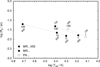 |
Fig. 2 Positions of hot-bubble formation in a Teff-R2 diagram for three different ‘families’ of the simulations from Table 2 (see legend). The numbers along the symbols are the usual mass-loss rate factors of the simulations, while the tilted numbers indicate the wind velocity (in km s−1) at the moment of hot-bubble formation. The dotted lines connect members of the same family. |
3.2 Bubble evolution
Once a hot bubble has formed, the further evolution depends on whether heat conduction occurs within the bubble or not. Figure 4 in SSW illustrates how heat conduction changes the structure of the bubble. Without heat conduction, the bubble is very hot (≳10 MK) and very diluted, and radiation cooling is negligible. The typical temperature and density profile set up by thermal conduction across the bubble results in a relatively cool and dense region at the bubble’s surface where radiation cooling may not be negligible anymore. It depends on the balance between the energy input by the stellar wind and the loss by radiation whether the bubble is stable and can expand further towards the evaporating stage. If radiative losses exceed the energy input, evaporation stops and may even turn into ‘condensation’ out of the bubble (Borkowski et al. 1990) with a possible reduction of the bubble mass if condensation exceeds the mass input by the stellar wind. SSW showed that (i) radiation-cooling of hydrogen-rich heat-conducting bubbles is unimportant and (ii) the evaporated mass soon dominates the whole bubble mass. Only because of evaporation are the models able to explain the observed X-ray luminosities of the bubbles around O-type central stars.
In contrast, the mass evolution of bubbles with a hydrogen-poor WR chemical composition is strongly dependent on radiative line cooling, for two reasons:
- 1.
The much higher line-cooling efficiency of the WR matter, already discussed above. Most relevant are the carbon ions C+4 and C+5 at about 1 MK and the oxygen ions O+6 and O+7 at about 2 MK because of their high abundances in a hydrogen-poor WR plasma (cf. Table 1).
- 2.
Because of the reduced thermal conduction efficiency, the temperature increases more steeply inwards than in hydrogen-rich bubbles. Hence, the matter is more concentrated towards the bubbles’ low-temperature and denser surface layers where cooling is generally most efficient.
In the following, we describe the evolution of two representative simulations, WR100V05 and WR100V05x5.5, as depicted in Fig. 3. These models were found to be most relevant for interpreting the observations (cf. Sect. 6).
The hot bubble of the WR100V05 simulation forms out of the radiatively controlled stage (case 1) at Teff≃50 000 K. At first, the hot bubble is only fed by the (hydrogen-poor) stellar wind. Evaporation starts later, approximately between 60 000 and 70 000 K, but at a very low pace because the plasma temperature close to the bubble’s surface is around 2 MK where cooling by O+6 and O+7 is very efficient. Beyond Teff = 70 000 K, the WR100V05 bubbles get so hot that radiation cooling decreases and the cooling time soon exceeds the bubble age (case 3). Evaporation of hydrogen-rich nebular matter dominates over the mass fed by the stellar wind to such an extent that the hydrogen-rich matter makes already up for 62% of the total bubble mass at maximum stellar temperature.
The temperature profiles of three selected bubbles from the WR100V05 simulation are shown in Fig. 4. The top panel contains a still radiative bubble (R1 ≃ R2) with a peak temperature well below 2 Mk where we have strong cooling by O+6 and O+7. The middle panel shows a moment after bubble formation where the bubble’s dense layers close the surface have T ≲ 2 MK, and evaporation is still suppressed by strong radiation cooling (case 2). Finally, the bubble temperature becomes very hot also at the surface, so that evaporation is now in progress (bottom panel). The WR-PN transition started to move from the bubble-nebula interface into the bubble’s interior (dashed vertical line).
The WR-PN abundance transition is defined as the radius where the helium to hydrogen ratio n(He)/(n(H) = 0.255, corresponding to a chemical composition obtained by mixing equal amounts (by mass) of PN and WR matter. Of course, the transition from hydrogen-poor to hydrogen-rich matter is not sharp due to numerical diffusion. Nevertheless, we assume a discontinuous chemical profile when computing synthetic X-ray properties with CHIANTI.
Figure 3 also shows the mass evolution of the hydrogen-rich PN1 bubbles (asterisks) for comparison. Although bubble formation and evaporation begin much earlier, the total bubble masses remain nearly a factor of ten lower than those of the WR100V05 bubbles. The high mass-loss rate inherent to the WR100V05 models more than compensates for the late bubble formation and the even later start of evaporation.
The bubble evolution of the ‘accelerated’ WR100V05x5.5 simulation is different. As expected, the higher wind densities for given Teff lead to a somewhat delayed bubble formation (Teff ≃ 65 000) K and beginning of evaporation (Teff ≃ 80 000 K). Because of the fast evolution, the bubble mass remains correspondingly smaller, especially also the evaporated hydrogen-rich mass (see Fig. 3). At the end of our simulation, the hydrogen-rich bubble part makes up for about 40% of the total mass.
Based on these hydrodynamical simulations of hydrogen-poor bubbles we come to the following conclusions:
After a bubble with WR chemical composition has formed, it can remain hydrogen-free for some time thanks to efficient radiation cooling that does not allow appreciable evaporation. For the particular case of our WR100V05 simulation, the chemically homogeneous stage persists for about 1500 yr. The existence of chemically homogeneous hydrogen-poor bubbles is therefore not necessarily an indication that heat conduction is suppressed (by whatever means).
However, once evaporation has started the WR bubble becomes quickly chemically stratified by evaporated nebular matter, and rather soon the hydrogen-rich mass fraction may even exceed the WR matter fraction provided by the stellar wind. The hot bubbles of old PNe with a WR-type central star are therefore expected to show signatures of a chemical stratification.
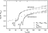 |
Fig. 3 Evolution of different parts of the bubble mass with stellar temperature Teff for the simulations WR100V05 and WR100V05x5.5. The total X-ray-emitting bubble mass is MX = MWR + MPN, where MWR is the mass contributed by the stellar wind and MPN that of the evaporated nebular matter. The symbols mark the models for which the data were evaluated. The evolution of MX(PN1) of the hydrogen-rich PN1 reference simulation is shown for comparison (asterisks). The three bubble models of the WR100V05 simulation whose temperature profiles are displayed in Fig. 4 are marked along the top abscissa. |
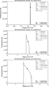 |
Fig. 4 Radial temperature profiles of three typical bubbles of the WR100V05 simulation. From top to bottom, the models represent case 1 (Teff = 44 000 K), case 2 (Teff = 56 000 K), and case 3 (Teff = 80 000 K, with beginning evaporation). The central star is at r = 0 cm. The vertical dashed lines mark the transition from the hydrogen-poor WR (left) to the hydrogen-rich PN chemistry (right). The bubble parameters like characteristic X-ray-temperatures, X-ray luminosities, and masses (for the entire bubble and for the respective subregions with the WR or PN composition) are given in the legends. The symbols on the bubble’s temperature profile mark different characteristic temperatures: of the entire bubble (diamond), the hydrogen-poor part only (star), and the hydrogen-rich evaporated part only (plus). |
3.3 The ionisation inside a wind-blown bubble
The implicit assumption commonly used for the interpretation of nebular X-ray emission is that the hot plasma within a windblown bubble is in CIE; that is, ionisation due to electron collisions is in equilibrium with radiative recombinations. In this case, the ionisation structure depends only on the temperature structure and adjusts instantaneously to any spatial and temporal variations. It can easily be seen, however, that the physical conditions within a tenuous hot bubble are far from favourable for the establishment of CIE (see, e.g. Liedahl 1999). First of all, we are dealing with a very rarefied entity with correspondingly long ionisation/recombination timescales. Furthermore, the electron temperature jumps by orders of magnitude when the wind matter crosses the inner wind shock, which makes it difficult for the ionisation to adjust quickly to the local temperature. Also, the flow of matter inside the bubble encounters a radially decreasing (or increasing) plasma temperature (cf. Fig. 6) that can drive ionisation away from CIE. Phases of very strong departures from equilibrium ionisation are expected (i) during the early bubble evolution where the mean bubble temperature increases quite rapidly, and (ii) when the stellar luminosity and the wind power drop while the star settles onto the white-dwarf sequence.
Indeed, our hydrodynamics simulations clearly show that NEI is the prevailing situation within a wind-blown bubble. This concerns especially the early radiative stage but more or less all following evolutionary phases as well. As an example, we show in Fig. 5 the ionisation fractions of the important elements carbon, oxygen, and neon for the NEI case (top) and the corresponding NEI to CIE number density ratio (bottom). We selected the same model of the WR100V05 bubble sequence that is also depicted in Fig. 6 below. It belongs to a late evolutionary phase where (i) the mean bubble temperature does not change rapidly, and (ii) the evaporation of PN matter is already quite efficient. Therefore this model allows us to disentangle the influence of chemistry and flow of matter on the ionisation in the hot bubble. Inspection of the figure reveals two regions that are especially prone to non-equilibrium ionisation:
downstream of the wind shock (post-shock region) where the rather cool and only photo-ionised wind matter must adjust to the now very high electron temperature, and
behind the conduction front where the relatively cool evaporated matter flows inwards, facing a steadily increasing electron temperature.
The only possibility to achieve or come close to the CIE conditions is given when the matter has left these two more extreme regions. But we see also that there are differences from element to element. Carbon has the lowest number of ionisation stages of the elements considered here and reaches full ionisation under CIE conditions in most parts of the bubble. Departures only occur in the post-shock region and behind the conduction front where C+5 dominates (cf. left panel of Fig. 5), but large regions in the bubble interior are close to CIE.
In the case of oxygen with its two additional ionisation stages (middle panel of Fig. 5), the region where CIE is a good approximation shrinks considerably with respect to carbon. The whole bubble part containing evaporated matter (r > 4.5 × 1017 cm) is in non-equilibrium, and only the inner region containing hydrogen-poor wind matter is practically in ionisation equilibrium. Presumably, the relatively high electron density, in conjunction with the high oxygen abundance, favours CIE.
The deviations from CIE are even more extreme for neon: only in a very small region centered at (r ≈ 4 × 1017 cm) are all ionisation stages reasonably close to the equilibrium values predicted by CHIANTI (Fig. 5, lower left panel).
We conclude that the ionisation of wind-blown PN bubbles is, in general, far from CIE. The differences between the CIE and NEI cases depend on the element and are generally smaller in the central regions of high electron density and/or low flow velocity. The general trend is that the NEI ionisation always lags behind the CIE predictions. As will be shown below, the X-ray emission depends critically on the details of the ionisation structure inside the bubble. Since all previous interpretations of the diffuse X-rays from wind-blown bubbles assumed ionisation equilibrium, we provide both CIE and NEI results in the present work.
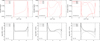 |
Fig. 5 Ionisation structure of the WR100V05 model displayed in Fig. 6. The upper panels show the radial profiles of the NEI ionisation fractions for the last four ionisation stages of carbon (left), oxygen (middle), and neon (right) as computed with NEBEL/CORONA. The NEI to CIE logarithmic number density ratios are plotted in the respective bottom panels. The wind shock is at R1 = 2.5 × 1017 cm, the bubble’s surface (conduction front) at R2 = 6.5 × 1017 cm. |
3.4 The structure and X-ray emission of chemically stratified heat-conducting bubbles
Here we present an overview of the typical structure of a heat-conducting, wind-blown bubble with stratified chemical composition. As an example, we render in Fig. 6 the full radial structure of a complete hydrodynamical model (top) and its X-ray surface brightness as function of the impact parameter (middle and bottom), taken from the WR100V05 sequence close to the maximum of the stellar temperature at Teff ≃ 146 000 K.
The top panel encompasses the freely expanding wind, the hot bubble proper consisting of shocked wind and evaporated nebular matter, and the nebular structure. Because the bubble is isobaric, the different element mixtures produce jumps of the ion and electron densities at the composition transition.
Contrary to the particle densities, the run of the electron temperature is smooth across the composition change (red dashed line in the top panel of Fig. 6). However, there is a very small change of the gradient at the position of the composition change.
The temperature profile is a bit steeper in the hydrogen-poor part of the bubble because of the lower heat-conduction efficiency of the hydrogen-poor WR composition. A detailed discussion how the heat-conduction efficiency and the bubble’s temperature structure depends on the chosen element composition is given in Papers I and II.
The synthetic X-ray brightness distributions shown in the middle and bottom panels of Fig. 6 clearly reflect the two different chemistries: The outer, hydrogen-rich part is significantly fainter than the inner part containing the WR matter. The reason is the much higher X-ray emissivity of the WR plasma with its high mean electronic charge of Z ≃ 4. The shape of the brightness profile and its absolute magnitude depend sensitively on the treatment of ionisation. Assuming non-equilibrium ionisation (on the basis of our hybrid approach outlined in Sect. 2.1) we see a geometrically extremely thin ‘spike’ of very high X-ray intensity immediately behind the wind shock at R1 = 2.5 × 1017 cm (bottom). This is the signature of the post-shock transition region where the shock-heated gas is still far from being in ionisa-tion equilibrium. Closer inspection reveals that line emission of C V at 34.97 and 40.27 Å, originating from a C+5 ‘pocket’ just behind the reverse wind shock, is primarily responsible for this emission spike, with minor contributions of O VII lines. Unsurprisingly, the intensity spike disappears when CIE is assumed (middle panel).
Observationally, the (intrinsic) intensity distribution is distorted by extinction because the low-energy X-rays from the cool outer bubble regions are more affected by absorption than the high-energy X-rays from the hot inner parts. The same holds for the post-shock intensity spike whose amplitude is significantly reduced after extinction (dashed line in bottom panel of Fig. 6) because the lower-ionised species emit preferentially at lower energies.
The dominant X-ray emission from the hotter WR bubble region has a profound influence on the mean bubble temperature. The definition of Eq. (1) leads to a formally much higher value of TX than for a chemically homogeneous bubble. The calibration of the mean bubble temperature against line ratios breaks down because both depend differently on the radial position of the chemical discontinuity within the bubble: TX is an emissivity weighted mean over the entire bubble whereas the spectrum is always dominated by the hotter, inner hydrogen-poor bubble part. We therefore determined separately the mean temperatures of both bubble parts and found, assuming NEI (CIE) for the bubble shown in Fig. 6, TX(WR) = 6.70 (5.86) MK and TX(PN) = 2.68 (2.87) MK, respectively. The characteristic temperature of the whole bubble is TX = 5.68 (5.18) MK, i.e. close to the mean temperature of the hydrogen-poor WR matter.
Observationally, only the mean temperature of the entire bubble can, in principle, be determined from the bubble spectrum, provided the chemical stratification is known a priori, which is usually not the case. A thorough discussion of how the spectral appearance of a bubble depends on the position of the WR-PN chemical transition can be found in Paper II (Figs. 16 and 17).
According to our models, the image of an evolved WR bubble with ongoing evaporation should consist of an X-ray-bright central region confined by a ring of very low emission (cf. Fig. 6, lower panels). The intrinsically bright but thin post-shock region will be difficult to detect given the limited spatial resolution and comparatively poor photon statistics of existing observations. This is especially true for the hydrogen-rich bubbles with their much lower carbon abundance.
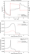 |
Fig. 6 Hot-bubble structure of the WR100V05 simulation at t = 9107 yr, Teff = 139 968 K, L⋆ = 2841 L⊙· Top: radial profile of electron temperature (dashed, right ordinate), electron density (dotted), and ion density (solid). The star is at r = 0, the wind’s reverse shock at R1 = 2.5 × 1017 cm. The transition from the wind-shocked hydrogen-poor WR matter to the evaporated nebular PN matter is at r = 4.6 ×1017 cm (T ≃ 5.0 MK), the heat conduction front (bubble-nebula interface) at R2 = 6.5 ×1017 cm, and the high-density region between 6.5 × 10¹⁷ and 8.3 × 1017 cm is the fully ionised planetary nebula proper with its double-shell structure and an electron temperature of about 1.2×10⁴ K. Middle: X-ray surface brightness distribution (6–11 Å) for the same model, assuming CIE, before (solid) and after (dashed) absorption by a hydrogen column density of NH = 0.25 × 1022 cm−2. The masses contained in the two bubble parts are 3.05 ×10⁻³ M⊙ of WR matter, supplied by the stellar wind, and 4.24 ×10⁻³ M⊙ of evaporated PN matter. Bottom: same as middle panel, but assuming NEI of nine key elements. |
Compilation of stellar and X-ray properties of the objects discussed in this paper.
4 Planetary nebulae with diffuse X-ray emission
In this section, we compile data of planetary nebulae with diffuse X-ray emission. With the advent of reliable distances provided by the Gaia satellite, we found it worthwhile to reevaluate the object parameters to put the following investigation and the conclusions of earlier publications (SSW, Ruiz et al. 2013) onto a firm basis.
Table 3 presents a compilation of the relevant parameters of the 12 planetary nebulae from which diffuse X-ray emission has been observed and analysed in the past. Seven have normal, hydrogen-rich O-type central stars (including NGC 6543 with spectral type ‘wels’), and five have hydrogen-poor central stars of various spectral types, all of which we refer to as of [WR]-spectral type for simplicity. Since our aim also is to relate stellar wind parameters with X-ray emissions of windblown bubbles, only objects for which both X-ray spectra and stellar wind data are available are included in the sample of Table 3. All of the listed objects are contained in the Gala Data Release 3 (DR3) and have parallax errors well below 10% in most cases3.
There are two objects for which the Gaia parallaxes appear to be questionable, at least: NGC 5315 and NGC 7026, both with a nucleus of [WR] spectral type. The Gaia distance to NGC 5315 of only 0.96 kpc leads to a (bolometric) stellar luminosity of about 670 L⊙, much too low for a post-AGB object with Teff = 75 000 K. We therefore decided to keep the distance recommendation of Marcolino et al. (2007) of 2.5 kpc that corresponds to a reasonable luminosity of 4900 L⊙ (Table 3). Our distrust is supported by the high renormalised unit weight error (RUWE) of the Gaia measurement, RUWE = 2.63, indicating a problematic result.
For the [WR] object NGC 7026, a Gala DR3 distance of 3.23 kpc (RUWE = 1.05) is reported, which in turn leads to a stellar luminosity of 62 000 L⊙, an unreasonably high value for a post-AGB object, well above the Chandrasekhar-limit of about 50 000 L⊙ for an electron-degenerate carbon-oxygen stellar core. However, the mass-loss rate, wind luminosity, and X-ray luminosity are high but still reasonable (cf. Cols. 7, 10, and 11 in Table 3). Since we are unable to resolve this discrepancy with our limited information, we adopted here the rather accurate Gaia distance. We note that the (bolometric) luminosity of NGC 7026’s nucleus is not needed for the present study.
Because of the generally rather small distance uncertainties provided by the Gaia measurements, we would have liked to get likewise accurate values for the stellar bolometric and wind luminosities. To this end, we investigated and compared more recent work based on sophisticated stellar atmosphere or pho-toionisation modelling methods. The relevant papers are also listed in Table 3, and appropriate averages of the parameters were derived for cases for which more than one paper was avaliable. We used only data from publications where next to the luminosities and mass-loss rates also the assumed distances were provided, which is not always the case. The distance-dependent quantities were rescaled to our adopted distances accordingly, i.e. the luminosities with d2 and the mass-loss rates with d1.5 (cf. Leuenhagen et al. 1996).
To our surprise, the determination of a reliable stellar luminosity appeared to be more difficult than believed: for given distance, the bolometric stellar luminosity, Lstar, may still differ by a factor of two between different authors! We believe that, next to systematic errors introduced by the quality of the modelling, an underestimated source of error is the extinction towards the object in question.
Altogether, the ‘intrinsic’ uncertainty of the bolometric luminosities listed in Table 3 may amount to about 30% (0.11 dex). If we consider this as a typical intrinsic luminosity uncertainty for all sample objects, the contribution of the distance uncertainty (≲10%) is comparatively small for objects with good Gaia distances.
The mass-loss rates (and therefore also the wind luminosities) are the most uncertain parameters: we found that the lowest and highest mass-loss rate of a particular object can differ by a factor of up to three. The typical error of the mean mass-loss rate in Table 3 is estimated to be about 60% (0.20 dex). As above, the low distance uncertainties do not significantly contribute to the mass-loss error.
However, we believe that the real mass-loss uncertainties are much larger by systematic effects. The rates listed in Table 3 are based on the assumption of a homogeneous wind flow. However, detailed line analyses showed that the winds may have inhomo-geneous structures. This kind of ‘clumping’ can be approximated by the so-called ‘volume-filling factor approach’. Although it is difficult to determine the filling factor f for individual cases, Hillier & Miller (1999) estimated that a value of 0.1 would be reasonable. Because the true mass-loss rate scales as Ṁ(f) = f1/2 Ṁ(f=1), clumping always reduces the mass-loss rate. For instance, a value of f=0.1 reduces the mass-loss rate by a factor of three (−0.5 dex).
These uncertainties of the mass-loss rates translate directly into the respective errors of the wind powers, Lwind = 0.5 Ṁwind  . The wind velocities can be measured from the absorption troughs of optically thick wind lines or the widths of emission lines and are much less uncertain. Although the velocity errors enter in quadrature, their contribution to the total error budget of the wind power is virtually negligible.
An important quantity in the context of this work is the bubble radius, R2, which is, by definition, identical with the inner nebula boundary. We measured the bubble sizes from the existing X-ray images, and in cases of elongated bubbles we took the geometrical average of their minor and major semi-axes. The derived bubble sizes are listed in Table 3, too. They agree, after distance adjustments, reasonably well with those presented in Ruiz et al. (2013)4.
Table 3 also contains the relevant X-ray data, i.e. observed X-ray luminosities LX and the characteristic X-ray temperatures TX. Both are taken from the compilation of Ruiz et al. (2013, Table 2 therein), rescaled to our distances, and refer to the energy range 0.3–2.0 keV (6.2–41.3 Å). The influence of the chosen X-ray band width on the values of LX and TX is discussed in Appendix A.
In general, the accuracy of the derived X-ray properties is limited by (i) the unknown column density of absorbing intervening matter, and (ii) the quality of the X-ray observations themselves (low-number photon statistics with total photon counts as low as about 30 in the quoted energy range). Though a reasonable determination of the X-ray luminosity is still possible (on the 20% level, extinction not considered), the determination of a meaningful X-ray temperature appears questionable. We therefore treat mean bubble temperatures based on spectra with photon counts of less than 100 with caution and give them in italics in Table 3 (Col. 13). This applies to IC 418, IC 4593, NGC 40, and NGC 6826.
5 Confronting our standard hydrogen-rich post-AGB simulations with the observations
In this section we compare the stellar and bubble parameters of the sample objects listed in Table 3 with the predictions of our existing post-AGB models which have already been used in SSW and Ruiz et al. (2013). However, we investigate here for the first time the effects of non-equilibrium ionisation on the characteristic properties of the X-ray emitting plasma, in comparison to the usual assumption of collisional ionisation equilibrium.
We follow the paradigm of single star evolution where extensive (spherical) mass loss along the AGB leads to the depletion of the stellar envelope, forcing eventually the star to leave the AGB. We note that the evolutionary calculations are valid for hydrogen-rich objects only.
Nevertheless, we include the [WR] objects in the comparison with the predictions of our hydrogen-rich post-AGB models. This will allows us to interpret any differences in the parameters of both type of objects (PN/WR) in physical terms, and will provide us with preliminary constraints on the evolution of the [WR] central stars by selecting the parameters of the new hydrodynamics simulations with WR-type winds that can reproduce the observed hydrogen-poor hot bubbles reasonably well (see Sect. 6).
5.1 Stellar luminosities and wind powers
The classical Hertzsprung-Russell diagram in the top panel of Fig. 7 shows that all the displayed sample objects are still on or very close to the horizontal part of their post-AGB evolution and are embraced by our 0.565 and 0.625 M⊙ post-AGB tracks.
The mean luminosity of the seven hydrogen-rich O-type objects is about 4900 L⊙, close to the luminosity of our 0.595 M⊙ model. This mean luminosity corresponds rather well with the mean luminosity of about 5000 L⊙ found for a sample of 15 nebulae with hydrogen-rich nuclei whose distances have been derived by the expansion-parallax method by Schönberner et al. (2018). The mean luminosity of the nine hydrogen-rich central stars in the Magellanic Cloud sample of Herald & Bianchi (2004, 2007) is 4200 L⊙. Considering the rather small sample sizes and the uncertainties inherent to the luminosity determination, the agreement between the mean stellar luminosities of these three samples is rather satisfying.
The mean luminosity of the four displayed hydrogen-poor [WR] central stars is about 6000 L⊙. This rather high mean luminosity is in contrast to the work of Herald & Bianchi (2004, 2007) on planetary nebulae in the Magellanic Clouds. Their MC sample contains three objects with hydrogen-deficient nuclei (the ‘odd’ object SMP LMC 83 neglected) whose luminosities range from about 2400 to 4200 L⊙, with a mean of about 3600 L⊙. However, both samples are really too small for a meaningful comparison between the Milky Way and MC [WR]-type central stars. A significant difference between the mean stellar luminosities of the O-type and [WR]-type sample objects is not evident.
However, a significant difference between O- and [WR]-type central stars i obvious if one considers their wind luminosities,  , (Fig. 7, bottom panel). A clear segregation between both samples is now visible. The observed wind luminosities of the hydrogen-rich O-type objects cluster around our four post-AGB tracks, but with a spread that is much wider than the spread of the model tracks (see also below). Nevertheless, the trend with stellar effective temperature is compatible with the predictions by Pauldrach et al. (1988).
In contrast to the O-type central stars, the [WR]-type objects have systematically much higher wind luminosities, varying between about 102… 103 L⊙ over the whole temperature range. If NGC 5189 (no. 7) is ignored, there appears to be a similar trend with Teff, too. A fair match to the observed values of the five [WR]-type sample objects can be achieved if the wind power of our 0.595 M⊙ post-AGB reference model is increased by a factor of 50 (dashed line in the bottom panel).
Figure 8 disentangles how the wind power of our sample objects is composed of wind velocity (top) and mass-loss rate (bottom). The wind velocities of the hydrogen-rich sample objects follow, on the average, closely the predictions of our models based on Pauldrach et al. (1988). Only the wind velocity of NGC 2392 (no. 5) is far too low. In contrast, the wind velocities of our [WR]-type objects are systematically lower (NGC 5315, no. 8, excepted) by a factor of about two (cf. dash-dotted line in the top panel).
This result is in agreement with the findings in Paper I. Based on a sample of 13 [WR]-type central stars which contains only BD +30°3639 and NGC 40 from our sample, the authors found that the Pauldrach et al. (1988) wind velocities derived for hydrogen-rich central stars must be reduced by a factor of 0.583, on the average. This result is at variance with the computations of Pauldrach et al. who found, for given Teff, higher wind velocities for hydrogen-poor central stars. However, these authors used simple hydrogen-poor model atmospheres without enhanced carbon and oxygen abundances. Based on these findings, we will consider only the simulations WR#VO5 as relevant for interpreting the properties of the observed bubbles around hydrogen-poor central stars.
Concerning the mass-loss rates (bottom panel of Fig. 8), the model predictions are consistent with the observations of our sample O-type stars. The scatter is very high, probably indicating (i) that either the observed mass-loss rates are more uncertain than generally believed or (ii) that our understanding of radiation-driven mass loss needs revision. This mass-loss scatter is obviously responsible for the scatter of the wind power seen in Fig. 7 (bottom panel).
The bottom panel of Fig. 8 indicates that the mass-loss rates of our [WR]-type central stars are significantly higher than for their O-type counterparts. The hydrogen-poor wind models of Pauldrach et al. (1988) are unable to explain the high mass-loss rates of [WR]-type central stars. Nevertheless, they are astonishingly well matched by scaling up the standard mass-loss rates of the Pauldrach et al. (1988) wind of our 0.595 M⊙ post-AGB model by a factor of 200. The combination of this mass-loss enhancement with the Pauldrach et al. wind velocities halved leads then to wind powers of our [WR]-sample objects which are about 50 times higher than for our 0.595 M⊙ reference model (cf. bottom panel of Fig. 7).
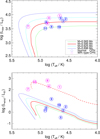 |
Fig. 7 Evolution of stellar energy output of four AGB models with remnant masses of 0.565, 0.595, 0.625, and 0.696 M⊙ (already used in SSW and Ruiz et al. 2013) versus their effective temperatures. The ‘reference’ track of Fig. 1, 0.595 M⊙, is highlighted by a thick red line. The positions of the objects from Table 3 are labelled with the object’s number within either a circle (O-type central star) or a hexagon ([WR]-type central star). Top: stellar bolometric photon luminosity; NGC 7026 (no. 12) falls outside the plotted luminosity range. Bottom: wind luminosity of the same AGB-remnants; NGC 7026 is now included. Solid tracks refer to the ‘standard’ mass-loss model ṀPPKMH (Pauldrach et al. 1988, see Sect. 2). The dashed track corresponds to a 0.595 M⊙ model with the wind power increased by a factor of 50 (see text). |
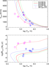 |
Fig. 8 Stellar-wind velocities (top) and mass-loss rates (bottom) versus stellar Teff for the same post-AGB tracks and sample objects as in Fig. 7. The dash-dotted line in the top panel represents the wind velocity of the 0.595 M⊙ model halved, the dashed line in the bottom panel the mass-loss rate of the 0.595 M⊙ model increased by a factor of 200. The positions of the objects no. 6 (NGC 3242) and no. 8 (NGC 5315) nearly coincide in the top panel, and those of no. 5 (NGC 2392) and no. 10 (NGC 6826) in the bottom panel. |
5.2 Bubble sizes
Another important aspect of post-AGB evolution is the speed of the central star across the HRD which is heavily mass dependent and cannot be disentangled in the Figs. 7 and 8. The post-AGB age of a particular planetary nebula is difficult to determine from its size and the nebular ‘expansion’ velocity. An in-depth discussion of the various methods used in the literature to estimate post-AGB ages and their systematic uncertainties can be found in Schönberner et al. (2014).
Here we avoid ages at all and use instead the bubble size, R2, defined by the radial position of the bubble-nebula interface, together with the stellar temperature as a marker of the bubble’s evolution across the HRD. The use of Teff instead of the post-AGB age has two advantages: (i) the Teff range does not vary much with remnant mass, and (ii) Teff is an observable quantity.
The expansion of bubbles formed by stellar winds colliding with the interstellar medium has been studied extensively by Weaver et al. (1977). They showed (their Eq. (21)) for the only interesting case of constant wind power and constant ambient (interstellar) medium that the bubble’s expansion with time depends weakly on wind power or ambient matter density. The expansion velocity decreases with time and comes eventually to a halt when the bubble’s thermal pressure equals that of the ambient, snow-ploughed matter. However, the results of Weaver et al. (1977) cannot be applied to bubbles inside expanding planetary nebulae. Here we have an accelerating wind power combined with a radially decreasing ambient matter density which is also strongly modified by ionisation.
This deficiency was eliminated by the work of Zhekov & Perinotto (1996). These authors approximated the post-AGB evolution of Blöcker’s (1995) 0.605 M⊙ model including the mass-loss rates by analytical expressions. The outer boundary condition was described by a slow (AGB) wind with constant mass-loss rate and velocity. Solving the relevant equations, Zhekov & Perinotto found for the expansion of an adiabatic bubble (their Eq. (2))
 (5)
(5)
where  is the central star’s wind power at t = t0 = 1000 yr, Ṁagb and Vagb the (constant)5 AGB-wind mass-loss rate and (terminal) velocity, and t is the bubble’s age. In contrast to the interstellar case, the bubble now expands into a surrounding medium whose density decreases with distance from the star: ρ(r) = Ṁagb/(4πVagb r2). Of course, Eq. (5) is only valid for the horizontal part of evolution across the HRD.
The time dependence of R2 in Eq. (5) ensures that the bubble’s expansion is always accelerated during the evolution across the HRD, in contrast to the Weaver et al. (1977) case where R2 ∝ t0.6. It is noted that the acceleration of the expansion slowly decreases with time,  . According to Eq. (5), the size evolution of the bubble depends rather weakly on the wind power and the AGB wind parameters, but such that the bubble expands faster for higher central-star wind power and lower AGB wind densities, or vice versa.
The sensitivity of the R2(Teff) relation on the central-star evolution is demonstrated in Fig. 9 for the four post-AGB simulations used in the Figs. 7 and 8. The curves of the 0.565, 0.595, 0.625, and 0.696 M⊙ models run nearly parallel and are well separated by about 1.7 dex in total. The main reason for this separation in the R2-Teff plane is the strong dependence of the evolutionary speed across the HRD on stellar mass. For instance, our post-AGB tracks have crossing times6 of about 800 yr (0.696 M⊙), 10 000 (0.595 M⊙, Fig. 1) and 20 000 yr (0.565 M⊙), i.e. a factor of about 25 between 0.696 and 0.565 M⊙, or 1.4 dex. The corresponding increase of the wind power from the 0.565 to the 0.696 M⊙ model is with a factor of about 2.5 only rather modest (cf. Fig. 7, bottom panel) and influences only little (−0.13 dex) the separation of the bubble sizes. Similarly, the influence of the density term in Eq. (5) is quite small. For hydrogen-rich central stars, the bubble size R2 at given Teff is therefore an indicator of the evolutionary timescale.
However, if the wind power is increased to higher values typical for the [WR]-type central stars, the wind-power term in Eq. (5) becomes important and must be considered. For instance, an increase of the wind power of the reference simulation (0.595 M⊙) by a factor of 50 would increase the bubble size by a factor 3.7, provided the evolutionary time scale remains the same (dashed line in Fig. 9).
In principle, the HRD crossing time also depends on the mass-loss rate (Schönberner & Blöcker 1993; Blöcker 1995). The four simulations of the evolution of the bubbles around hydrogen-rich central stars displayed in Fig. 9 are fully consistent with their respective mass-loss rates. [WR]-type central stars have much higher mass-loss rates (cf. Table 3) which in turn would reduce their HRD crossing times. However, since the formation and evolution of the hydrogen-poor central stars are unknown, we also do not know a priori (i) their HRD crossing times and (ii) how these depend on stellar mass. We consider therefore the HRD crossing times of [WR]-type central stars as a free parameter, scaled to the crossing time of our 0.595 M⊙ reference model.
The distribution of our sample objects in Fig. 9 reveals evolutionary differences between the two central-star subsamples. With the exception of NGC 2392 (no. 5) and possibly IC418 (no. 2), the bubble sizes of the O-type central stars are remarkably close to the predictions of our 0.595 M⊙ reference sequence. The spread is much less than one would expect from the luminosity spread in the top panel of Fig. 7. This confirms our finding that, thanks to Gaia, we are in a situation where the uncertainties of the luminosity determinations are now the limiting factor, and not the distances.
We conclude, in conjunction with Figs. 7, 8, and 9, that the hydrodynamics simulations of wind envelopes around post-AGB models as described in Perinotto et al. (2004) provide a fairly good description of the evolution of hydrogen-rich AGB remnants in terms of evolutionary timescale, mass-loss rate, wind velocity, and hot-bubble formation and expansion.
Only NGC 2392 (no. 5) does not fit into this scheme. It has (i) a high-luminosity central star with (ii) a very low wind power due to the unusually low wind speed (Figs. 7 and 8, top panels), and (iii) a comparatively big bubble for the low central-star temperature (Fig. 9). The stellar luminosity is not consistent with the size of the bubble which corresponds better to our low-luminosity model of 0.565 M⊙. Needless to say that the low wind power cannot be responsible for the extraordinary bubble size. We can only speculate that the wind power of NGC 2392’s central star has been much higher in the past. We note that individual luminosities which led to our mean value of NGC 2392 listed in Table 3 show an unusually high spread, viz. a factor of 2.7 from the lowest to the highest value, where the lowest luminosity (Herald & Bianchi 2011) is consistent with our 0.565 M⊙ remnant. More work is certainly needed for clarifying the case of NGC 2392.
In contrast to our O-type sample, the distribution of the bubble sizes of the five hydrogen-poor [WR]-type objects seems to indicate more diverse evolutionary histories. Since all five objects have very similar wind powers (cf. bottom panel of Fig. 7) and because the influence of the outer boundary conditions are small, their evolutionary timescales must vary considerably. A detailed discussion of the properties of the [WR]-type objects in Fig. 9 is postponed to Sect. 6 where more appropriate hydrodynamical simulations are used.
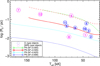 |
Fig. 9 Bubble radius, log(R2) versus central-star effective temperature, Teff, as predicted by our hydrodynamical simulations of the 0.565, 0.595 (PN), 0.625, and 0.696 M⊙ sequences together with the sample objects. The dashed line refers to that in Fig. 7 (bottom panel) and is an estimate based on Eq. (5) if the wind power of the 0.595 M⊙ model is increased by a factor of 50. The simulations are plotted from the beginning of bubble formation till maximum stellar temperature. |
5.3 X-ray properties
The hydrodynamical modelling of SSW showed that the bubble’s X-ray luminosity increases with time (or stellar temperature) because heat conduction leads to evaporation of nebular mass, resulting in a steady increase of the bubble mass with a corresponding increase of the X-ray luminosity. The increase of the X-ray luminosity with central-star mass is caused by the corresponding increase of the wind power which drives the evaporation, and the shorter evolutionary timescales resulting in a smaller bubble radius. Altogether, the volume emission measure, and hence the X-ray luminosity, of a hot bubble increases with stellar mass. When the stellar luminosity drops at the end of evolution, the wind power (and the evaporation) ceases, but the bubble continues to expand. Consequently, the bubble’s X-ray luminosity must fade, too. More details on the X-ray emission of heat-conducting wind-blown bubbles can be found in SSW.
In Fig. 10, the so-called X-ray HRD, the bubble luminosities of all sample objects are plotted as a function of stellar effective temperature and compared with the predictions of hydrodynamical simulations based on the post-AGB evolutionary sequences displayed in Fig. 7 (top panel). As expected from the above discussion, we see a considerable luminosity spread between the 0.565 and 0.696 M⊙ sequences of about 1 dex. We also see that the differences between NEI (top panel) and CIE (bottom panel) are comparatively small: the X-ray luminosities are in general higher in the NEI case by only about 0.1… 0.2 dex. These differences are too small to have any impact on the interpretation of the observations.
The mean X-ray temperatures behave differently and remain (0.696 M⊙ excepted) nearly constant for most of the post-AGB evolution (see Fig. 11). This temperature behaviour can be explained by Eq. (4) introduced in Sect. 2.2 and the wind model used in our hydrodynamics simulations: The increasing wind power, (Fig. 7, bottom) drives the expansion of the bubble such that the ratio of wind power over bubble size remains fairly constant or increases moderately (0.696 M⊙) during the horizontal evolution across the HRD. Both Tx and Lx drop at the end of our simulations as the wind power declines sharply while bubble expansion continues (cf. Eq. (4)). The general trend of increasing Tx-values with stellar mass is also explained by this equation: faster stellar evolution leads to smaller bubbles and, combined with a stronger wind, to higher bubble temperatures. Figure 11 also demonstrates that mean bubble temperatures do not differ significantly between the NEI and CIE cases. In all sequences (the 0.696 M⊙ sequence excepted), the NEI temperatures are a bit higher than the CIE temperatures, but by no more than about 0.2 MK.
From Figs. 10 and 11, we draw the following conclusions:
The observed X-ray luminosities and mean X-ray temperatures of the bubbles around O-type central stars and their run with effective temperature are well covered by the SSW hydrodynamical bubble models around AGB remnants between about ≲ 0.57 and 0.70 M⊙.
The bubbles around the [WR]-type central stars are systematically more luminous and would technically correspond to models with central stars of at least 0.63 M⊙, while their mean Tx values are comparable to the bubbles around O-type stars, albeit with a larger scatter.
The close correspondence between the X-ray and the classical HRD of the O-type objects is very gratifying since in Fig. 10 two different entities of the stellar-nebula systems are linked together: the star and its wind-blown bubble. For the [WR]-type sample objects, the stellar luminosities are very similar to those of the O-type objects, but the X-ray luminosities of their bubbles are definitively higher, obviously due to their much higher wind powers.
As the HRD does not contain any information on individual evolutionary timescales, it is instructive to use again the bubble radius instead of the stellar temperature as an independent indicator of the evolution of the X-ray properties, counting the time since bubble formation, which may vary from object to object because of different stellar masses, different wind densities, and radiation-cooling properties. As we have seen in Fig. 9, the size of the bubble, R2, is very sensitive to the stellar evolutionary timescale, and hence to the stellar mass.
Figures 12 and 13 show the X-ray luminosity and characteristic (mean) X-ray temperature Tx, respectively, versus bubble radius for our sample objects and the (hydrogen-rich) SSW bubble simulations. As already seen in Fig. 9, the dependence of the crossing timescale on remnant mass leads to a substantial horizontal spread of the individual simulations by more than an order of magnitude.
Thanks to the mass spread of the different bubble sequences seen in Figs. 12 and 13 we come to an even more detailed conclusion concerning the hydrogen-rich objects:
The X-ray luminosities of all seven bubbles around the O-type nuclei are constrained by our 0.565 and 0.625 M⊙ simulations, where six objects are closely reproduced by the 0.595 M⊙ model bubbles.
Virtually the same holds for the characteristic bubble temperatures if the very uncertain Tx value of IC 418’s bubble (no. 2) is ignored.
Altogether, the observed evolution of Lx and Tx of the bubbles around the O-type sample objects is fully in line with the existence of heat conduction with evaporation as introduced by SSW. Moreover, the observed increase of Lx with bubble radius by about two orders of magnitude and the observed moderate evolution of Tx seems to validate our models of hot bubbles around hydrogen-rich AGB remnants of around 0.6 M⊙, in particular their evolutionary timescales and the chosen mass-loss prescription. Nevertheless, any firm assignment of a particular object to one of the post-AGB sequences shown in Figs. 7 through 9 is problematic because of the uncertainties of the stellar luminosities (Lstar and Lx), and especially of the mass-loss rates.
In contrast, a consistent evolutionary picture is not evident for our [WR]-type sample objects.
There is no clear indication of an evolution of Lx with bubble size. The smallest two bubbles, nos. 1 (BD +30°3639) and 8 (NGC 5315), have X-ray luminosities that correspond well to the mean value of the three big bubbles, nos. 4 (NGC 40), 7 (NGC 5189), and 12 (NGC 7026), viz. log(Lx/L⊙) ≃ −1.0.
Concerning the mean bubble temperatures we can only state that the two young and small bubbles are relatively hot whereas the temperatures of the big bubbles are quite low, more comparable to those of the 0.565 M⊙ bubbles close to the end of our simulation.
Although the two samples are rather small, the obviously different X-ray properties of the bubbles around O-type and [WR]-type central stars suggest a diverse evolutionary history of these two central-star spectral types in general, and between the young and old [WR]-type objects in particular. Their different chemical compositions may certainly play a decisive role, too. For instance, the comparably low X-ray luminosity of the hydrogen-poor bubbles is in contrast to the prediction of Paper II, according to which bubbles with WR composition should have a 70–100 times higher X-ray luminosity than their hydrogen-rich counterparts. In order to tackle the problem of the comparatively low observed X-ray luminosities of hydrogen-poor bubbles, hydrodynamical models which allow for evaporation are mandatory. In the following section we therefore discuss our new simulations with hydrogen-poor winds in terms of their X-ray luminosities and temperatures.
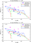 |
Fig. 10 X-ray HRD for our sample objects of Table 3 (symbols as in previous figures) together with the predictions of heat-conducting hydrodynamical bubble models around the 0.565, 0.595, 0.625, and 0.696 M⊙ sequences. The symbols (squares) along the sequences denote the individual models for which the X-ray emission has been computed by means of the CHIANTI software package. The top panel shows the NEI, the bottom panel the CIE case. |
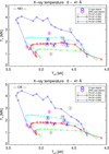 |
Fig. 11 Same as in Fig. 10, but for the characteristic bubble temperature Tx. The objects with very uncertain Tx values are shown in grey (Tx entries of Table 3 in italics). |
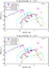 |
Fig. 12 X-ray luminosity versus bubble size of the sample objects listed in Table 3 (numbered symbols) together with the predictions of the four hydrogen-rich bubble sequences of the previous figures. Again, the NEI and CIE case is shown at top and bottom, respectively. |
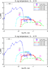 |
Fig. 13 Same as in Fig. 12, but for the characteristic bubble temperature Tx. The objects with very uncertain Tx values are shown in grey (Tx entries of Table 3 in italics). |
6 Our hydrogen-poor bubble models and the observations
Evaluating the global X-ray properties of the simulations with [WR]-type winds introduced in Sect. 3, it turns out that most of our simulations are of no relevance for interpreting the so far existing observations of the hydrogen-poor bubbles. Given the observed values of mass-loss rate and wind speed of the [WR]-type objects displayed in the Figs. 7, 8, and 9, we found that only the two simulations, WR100V05 and WR100V05x5.5, should suffice for a comparison with the observations. Our choice of a 100 times higher mass-loss rate only instead of 200 times as suggested by the observations if no wind clumping is assumed (Fig. 8, bottom) may be justified by assuming a moderately clumpy wind7 characterised by a volume filling factor of ƒ = 0.25.
6.1 Evolutionary stages
Figure 14 is the same as Fig. 9 but contains only the two selected WR simulations and the bubble positions of our [WR]-type sample objects. The conclusions concerning the evolution of [WR]-type central stars can be refined as follows:
The central stars of BD +30°3639 (no. 1) and NGC 5315 (no. 8) evolve fast and are fairly well represented by our accelerated WR100V05x5.5 simulation.
NGC 40 (no. 4) appears as having a central star which evolves more slowly than our WR100V05 sequence, viz. by a factor of about two (−0.30 dex).
The evolution of the bubbles of NGC 5189 (no. 7) and NGC 7026 (no. 12) is well matched by our WR100V05 simulation.
These conclusions remain valid even if one allows for the considerable uncertainty of the stellar mass-loss rates, mainly caused by the filling factor ƒ. For instance, an uncertainty of the mass-loss rate by a factor of three translates into an R2 change of +0.16 dex only, provided the other two terms in Eq. (5) remain virtually unchanged.
An important question still remains: are our models with WR-type winds and their delayed hot-bubble formation able to explain the existence of bubbles around the youngest objects of our [WR] sample, viz. of BD +30°3639 (no. 1) and NGC 5315 (no. 8)? Figure 14 contains the answer: we have marked the positions where the hot bubble forms (X) and where evaporation begins (x) for both simulations. Considering the uncertainties of individual stellar mass-loss rates (wind powers) and the corresponding changes of the times of hot-bubble formation and onset of evaporation, we can state the following:
The bubble of BD +30°3639 (no. 1) is close to the stage where our WR100V05x5.5 simulation predicts hot-bubble formation, while the bubble of NGC 5315 (no. 8) appears a bit more evolved, right before the beginning of evaporation. Both bubbles can therefore be considered to be chemically homogeneous with a hydrogen-poor WR composition.
The bubble of NGC 40 (no. 4) is still close to the evaporation stage and may already contain a small amount of evaporated hydrogen-rich matter.
The two most evolved objects, NGC 5189 (no. 7) and NGC 7026 (no. 12), should obviously have bubbles that are far into their evaporating stage. However, these objects with very extended bubbles show rather smooth X-ray intensity distributions which are not consistent with the model prediction of a sudden radial intensity drop towards an outer region of fainter X-ray emission next to the nebular rim as seen in Fig. 6.
Altogether, the observed parameter combination bubble size and stellar effective temperature found for our [WR]-type subsample can be matched by our simulations of hydrogen-poor bubbles if the wind power is selected appropriately and the evolutionary speed adjusted if necessary.
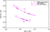 |
Fig. 14 Same as in Fig. 9 but now only for the new hydrogen-poor bubble sequences WR100V05 (upper) and WR100V05x5.5 (lower) together with the bubbles of the [WR] objects in Table 3. The black crosses indicate the moments of hot-bubble formation (big crosses) and the start of evaporation (small crosses). |
6.2 X-ray luminosities
Figure 15 shows the evolution of the X-ray luminosity with bubble size for the WR100V05 and WR100V05x5.5 simulations, again for both the NEI and CIE case. The NEI bubbles are more luminous than their CΓE counterparts, and the differences are a bit higher than seen above for the hydrogen-rich bubbles. The general trend is that the‘Overluminosity’ of the NEI bubbles is (i) higher during the earlier phases of evolution, and (ii) less pronounced for the ‘accelerated’ WR100V05x5.5 sequence. The higher bubble densities of the latter sequence obviously favour a bubble ionisation closer to equilibrium.
In general, the bubble evolution can be described as follows: When the hot bubble starts to form, its X-ray luminosity is already rather high, thanks to the high emissivity of the WR matter with 〈Z〉 ≈ 4. After this initial increase, the Lx evolution differs from the hydrogen-rich case. Instead of a continuous increase while the central star crosses the HRD, Lx remains fairly constant or even decreases with evolution. The reason lies in the fact that the bubble’s main mass input is due to evaporation of hydrogen-rich nebular matter which, however, contributes little to the total X-ray luminosity. For illustration, the individual luminosity contributions of the WR wind matter and the evaporated PN matter are separately shown for the WR100V05 sequence in Fig. 15. The input of hydrogen-poor wind matter is comparatively small and can hardly compensate for the decrease of the emission measure by expansion. We interpret Fig. 15 as follows:
The young and small bubbles around the nuclei of BD+30°3639 (no. 1) and NGC 5315 (no. 8) are again reasonably well represented by the young and still chemically homogeneous hydrogen-poor bubbles of our accelerated WR100V05x5.5 simulation (cf. Fig. 14).
The same holds for the bubble of NGC 40 (no. 4) if we shift the WR100V05 simulation by a factor of about 2.5 (0.4 dex) to the right, thereby approximating a slowed-down stellar evolution by a factor of 2.5 (arrow in Fig. 15). NGC 40 can then be explained as an object on the ascending part of the WR100V05 bubble sequence where bubbles are still (nearly) chemically homogeneous.
The X-ray luminosities of NGC 5189 (no. 7) and NGC 7026 (no. 12) are, within the uncertainties, fairly well represented by our WR100V05 bubbles during their evaporating stage.
It is very gratifying that both the Figs. 14 and 15 allow consistent interpretations concerning the present evolutionary stage of our [WR]-type sample objects with respect to bubble size and X-ray luminosity. It appears that our hydrogen-poor bubble sequences WR100V05 and WR100V05x5.5 somewhat overestimate the X-ray luminosities of our sample objects, suggesting that their real wind powers (mass-loss rates) are a bit lower than those assumed for the models. Nonetheless, our simulations do not indicate any evolutionary connection between the young and old [WR]-type sample objects, contrary to what one might have assumed from Fig. 10 alone.
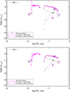 |
Fig. 15 Bubble X-ray luminosities Lx versus bubble radius R2 of the sequences WR100V05 (right, solid) and WR100V05x5.5 (left, dashed) and the bubbles of the [WR]-type sample objects of Table 3. Evolution occurs from left to right, and maximum stellar temperatures are indicated by a vertical mark. Evaporating bubble models are connected by a thick solid or dashed line. The WR100V05 bubbles also contain the information on the luminosity contributions of the hydrogen-poor WR part (crosses) and the evaporated hydrogen-rich PN part (triangles). The arrow indicates the (estimated) shift of the WR100V05 bubbles if the evolutionary timescale is increased by a factor of 2.5. The top panel displays the NEI, the bottom panel the CIE case. |
6.3 The characteristic bubble temperatures TX
In Fig. 16, the comparison between the X-ray temperature predictions of our WR100V05 and WR100V05x5.5 bubble sequences and the observation is presented, again separately for the NEI and CIE case. The mean bubble temperatures are systematically higher in the NEI case by about 0.5 MK at most.
The temperature evolution predicted by the models follows an inverted ‘U’ shape. First, the bubble temperature increases rapidly with bubble size, in pace with their X-ray luminosities (Fig. 15), goes through a maximum, and finally declines towards the end of our simulations. A longer lasting phase of roughly constant bubble temperature as found for the hydrogen-rich case is missing, obviously because the bubbles form much later at higher stellar temperatures and hence with bigger bubble radii. Furthermore, the achieved bubble temperatures are significantly higher than those of the hydrogen-rich bubble models (cf. Fig. 13). The reason is the very high stellar wind power at comparable bubble sizes (cf. Eq. (4)) which cannot be compensated fully by the higher bubble size R2 and its faster evolution.
Although the wind model is the same in both displayed simulations, the achieved bubble temperatures are quite different, i.e. 6.0 vs. ≃ 9.0 MK at maximum (NEI case). The reason is the faster stellar evolution of the WR100V05x5.5 simulation where the bubbles are smaller by about a factor of 5.5 and correspondingly hotter. An estimate using Eq. (4) yields a factor of 5.52/7 = 1.6, and therefore the maximum mean bubble temperature reached by the accelerated simulation should be 6.0 × 1.6 = 9.6 MK, in fair agreement with the simulation.
For completeness, we also show in Fig. 16 the mean temperatures of the hydrogen-poor and hydrogen-rich bubble parts of the WR100V05 sequence separately. The differences are considerable, simply because the evaporated hydrogen-rich matter resides in the outer, cooler parts of the bubble while the wind matter occupies the inner, very hot part of the bubble (cf. Figs. 4 and 6). However, the hydrogen-poor WR matter always dominates the X-ray emission and the overall mean bubble temperature TX is always below but close to TX(WR). We conclude from Fig. 16:
The mean bubble temperatures of the young objects BD+30º3639 (no. 1) and NGC 5315 (no. 8) are consistent with the prediction of the WR100V05x5.5 models with purely hydrogen-deficient composition and an accelerated stellar evolution.
The mean temperatures of the two old bubbles of NGC 5189 (no. 7) and NGC 7026 (no. 12) completely disagree with the predictions of the WR100V05 bubbles. They range between about 1.1 and 1.6 MK while the models predict temperatures of up to 5.6 MK in the relevant Teff regime. Even the evaporated, hydrogen-rich bubble regions have mean temperatures as high as about 2.6 MK. Concerning NGC 40 (no. 4), we repeat that any temperature estimate of bubble plasmas from spectral X-ray distributions requires observations of sufficiently high quality. In our opinion, this is not the case for NGC 40 where the total number of useful X-ray photons is around 60 only.
However, taking the observed low mean bubble temperature as granted, the following interpretation can be made. Assuming a slower central-star evolution as discussed above for interpreting the X-ray luminosity and size of NGC 40’s bubble, its low mean temperature would be a natural consequence (cf. arrow in Fig. 16). The hot bubble of NGC 40 would therefore be rather young and still chemically homogeneous but already quite big because of the slow central-star evolution.
The obvious mismatch between theory and observation found for the bubble temperatures of NGC 5189 and NGC 7026 is surprising in view of the rather good agreement concerning their bubble sizes and X-ray luminosities. It is certainly real because the spectral appearance of a 5 MK hot plasma with WR composition can by no means be mistaken with that of a plasma as cold as about 1.6 MK or less. Apparently, our 1D hydrodynamical NEBEL simulations are missing some physical ingredients that are necessary to provide an adequate description of evaporating hydrogen-poor wind-blown hot bubbles.
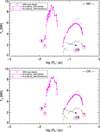 |
Fig. 16 Characteristic X-ray temperature TX versus bubble radius R2 for the sequences WR100V05 (right, solid) and WR100V05x5.5 (left, dashed) and the bubbles of our sample (Table 3). Again, bubble evolution occurs from left to right, and maximum stellar temperatures are indicated by a vertical mark. Evaporating bubbles with inhomogeneous composition are connected by thick solid or dashed lines. The mean temperatures of the hydrogen-poor part, TX(WR), and of the hydrogen-rich part, TX(PN), are shown as crosses and triangles, respectively, for the WR100V05 bubbles. As in the previous figure, the arrow indicates the (estimated) shift of the WR100V05 bubbles if the evolutionary timescale is increased by a factor of 2.5. The symbol of NGC 40 (no. 4) is shown in grey because of the large uncertainty of the derived TX value. The top and bottom panel displays the NEI and the CIE case, respectively. |
7 Discussion
The present study, a follow-up of the SSW and Ruiz et al. (2013) works, shows again the usefulness of our 1D hydrodynamical code NEBEL/CORONA in conjunction with the heat conduction paradigm for interpreting the soft X-ray emission from the windblown bubbles of planetary nebulae. For computing synthetic X-ray spectra, we have for the first time allowed for deviations from collisional ionisation equilibrium for nine key chemical elements that dominate the emission in the considered energy range. The comparison of the NEI results with those based on the usual assumption of CEI revealed considerable differences of the local ionisation fractions inside the bubbles. Concerning the global bubble parameters like X-ray luminosity and characteristic X-ray temperature, the differences between the NEI and CIE cases are less dramatic, and therefore the previous conclusions based on the CIE alone remain valid. In contrast, the determination of abundance ratios from spectral features will depend critically on the details of the ionisation balance.
While the diffuse X-ray emission of wind-blown bubbles around hydrogen-rich central stars could be very well explained in all aspects by our simulations, open questions still remain for bubbles around [WR] central stars where the models predict the extended bubbles to become chemically inhomogeneous due to evaporation of hydrogen-rich nebular matter. We will discuss some important issues in the following.
7.1 The importance of mixing by dynamical instabilities
For the hot bubbles around hydrogen-rich central stars, we can compare the observed X-ray temperatures with the predictions of the pure mixing models of Toalá & Arthur (2016). For central-star masses around 0.6 M⊙ relevant here, the pure mixing models reach rather high mean bubble temperatures from about 2.6 up to about 4 MK in the stellar temperature range from about 40 000 to 100 000 K (cf. Fig. 8 in Toalá & Arthur 2016). Although this stellar temperature range is almost covered by our sample objects (cf. Table 3), such high bubble temperatures are not observed: With the exception of IC 418 whose TX value is uncertain and which also has most probably a more massive central star, the TX values of the six remaining bubbles do not indicate any evolution with bubble size or stellar temperature (Fig. 13). Instead, they cluster around the mean value of 1.96 ± 0.25 MK, very close to the mean bubble temperatures of our 0.595 M⊙ sequence, viz. ≃1.8 MK.
Regarding the question about the role of dynamical mixing, this mismatch suggests that mixing processes as considered by Toalá & Arthur (2016) cannot alone be responsible for the observed low mean bubble temperatures. The reason is that mixing is a slow process; the time needed for producing enough relatively cool bubble matter seems to be comparable to the HRD crossing time. In contrast, thermal conduction works on an extremely short timescale and imposes the typical temperature profile nearly ‘instantaneously’ (Zhekov & Perinotto 1996). Indeed, if Toalá & Arthur (2016) also allow for thermal conduction in their simulations, the mean bubble temperature of their 0.597 M⊙ sequence does not exceed 1.6 MK.
7.2 Low mean temperatures of hydrogen-poor bubbles
Our bubble models with thermal conduction are able to explain the rather moderate mean temperatures of the young bubbles of BD+30º3639 and NGC 5315 but fail in the case of large, old bubbles (e.g. of NGC 5189 and NGC 7026). The reason for this failure is evaporation of hydrogen-rich nebular matter during later stages which leads in our models to a chemical stratification where the evaporated matter encloses the hydrogen-poor wind matter. These chemically stratified bubbles have very high mean plasma temperatures since the X-ray spectrum is always dominated by the emission of the hydrogen-poor but hot inner bubble region.
Such high temperatures have so far not been observed, suggesting that in nature an additional physical process is at work that somehow prevents a clear separation of the two chemistries within a bubble. Dynamical mixing across the chemical discontinuity by hydrodynamical instabilities is certainly conceivable. Complete mixing would result in (i) a lowering of the mean ionic charge, (ii) a surface-brightness distribution without a jump, and therefore (iii) a lower characteristic X-ray temperature. However, a more thorough investigation of this scenario is beyond the scope of the present work.
Another possibility is a sudden considerable decrease of the wind power (cf. Eq. (4)) during the late stages of evolution. However, this is not observed: the present-day wind-powers of NGC 5189 and NGC 7026 correspond closely to those used in our models (Fig. 7, bottom panel, dashed line).
Finally, we would like to emphasise that the mean X-ray temperature derived from the observation and from the models, respectively, are based on different methods. The usual method used to interpret the observations is to fit spectral features assuming a single-temperature plasma, while the X-ray temperature of the models is defined as the emissivity-weighted temperature of the heat-conducting bubble structure. Hence the characteristic mean temperatures derived from the models are not directly compatible with those derived from the observations. However, it was shown in Paper II (Fig. 6 therein, albeit assuming CIE) that the differences are quite moderate and - in CIE - do not exceed 0.4 MK in the relevant temperature range, in the sense that the bubble models predict lower temperatures for given line ratios. Therefore, this inconsistency cannot be held responsible for the temperature discrepancies discussed here.
7.3 The problem of wind clumping
As mentioned previously, especially the dense winds of the [WR]-type objects may not be homogeneous but rather ‘clumpy’. However, we neither can model clumpy winds nor can we estimate the consequences of wind clumping. These uncertainties of the mass loss from [WR]-type central stars are the main reason why we did not perform simulations which provide individual matches to our sample objects. Fortunately, any uncertainties of the mass-loss rate, and hence wind power, by factors of 2….3 only have a rather modest influence on the bubble’s size, X-ray luminosity, and mean temperature, and would not change our interpretations and conclusions.
It is possible that the hot bubble has density inhomogeneities (‘clumps’) as well because a clumpy wind flow becomes simply compressed and decelerated while passing through the shock. High-density regions within a bubble would be sites of very efficient radiation cooling, reducing thereby considerably the part of the wind power capable of heating the bubble. However, it is unclear how such density fluctuations could survive under the conditions of constant pressure and thermal conduction. Based on 2D hydrodynamical models, Dwarkadas (2023) recently put forward the idea of additional bubble cooling by density inhomo-geneities in order to explain the low temperatures of wind-blown bubbles around massive stars. He concluded that the inclusion of thermal conduction is not necessary to reproduce the X-ray temperatures and spectra. On the other hand, Zhekov & Park (2011) and Zhekov (2014) had previously demonstrated that heat conduction is an efficient physical mechanism controlling the temperature structure in 1D numerical models of this type of hot bubbles, and therefore a viable explanation of the low plasma temperatures deduced from the observed X-ray spectra of both massive WR-type stars, as is the case for planetary nebulae.
7.4 The chemical composition of hydrogen-poor bubbles
By using the WR abundances of Table 1 in our simulations with hydrogen-poor stellar winds it is guaranteed that, at least in the beginning, the bubbles are truly hydrogen-poor, too. The hydrogen-poor character of our WR mixture is evident from the numbers in Table 1 where helium and carbon are the most abundant species.
This is obviously not the case in Table A1 of Toalá & Arthur (2018) where the abundance values of BD+30°3639 indicate that hydrogen and helium are still the most abundant elements (ϵH = 12, ϵHe = 10.99, ϵC = 10.59, ϵO = 9.53). The abundance of carbon, oxygen are scaled relative to helium according to the ratios found by Marcolino et al. (2007) and Yu et al. (2009). This procedure ensures that helium, carbon, and oxygen have the correct proportions, but the chemical mixture is still hydrogen-rich, at variance with existing spectral analyses which proved that BD +30°3639’s surface is definitively hydrogen-poor (e.g. Leuenhagen et al. 1996; Marcolino et al. 2007). Such an element distribution ignores the fact that the surface layers of [WR]-type central stars consist of matter that has gone through hydrogen and helium burning in the past.
Since hydrogen and helium have no X-ray line signatures, such a ‘pseudo’ hydrogen-poor composition is able to provide correct X-ray spectra once the proportions of the main X-ray emitters, carbon, oxygen, and neon have been adjusted accordingly. However, the ‘pseudo’ hydrogen-poor composition has a lower mean electronic charge than a true WR mixture (4.4) and is therefore not suited to compute realistic X-ray luminosities and cooling rates of hydrogen-poor hot bubbles.
7.5 Formation scenarios of hydrogen-poor central stars
We have assumed here, based on single-star simulations, that the change to a hydrogen-free (-poor) stellar surface occurs immediately when the star leaves the AGB, possibly by a thermal pulse right at the tip of the AGB. A thermal pulse occurring later while the AGB remnant evolves across the HRD, is no real option for the following reasons:
Such a thermal pulse (late or very late) forces the star to expand back to the tip of the AGB for some time until it shrinks again towards hotter regions of the HRD. During this second giant phase, a deep envelope mixing is responsible for the hydrogen depletion of the surface layers. Possible examples of such a scenario are, e.g. A 30 (Guerrero et al. 2012) and A 78 (Toalá et al. 2020). However, none of the three evolved objects in our [WR]-type sample show indications of nested nebular shells with different chemistries. Also, the existence of [WR]-type central stars as cold as ≃20 000 K (Fig. 2 in Hamann 1997), seem to support our assumptions.
There remains the possibility of binary-star interactions which may lead to the loss of the remnant’s hydrogen-rich envelope. However, this should occur only while the object in question is big, i.e. still on or close to the tip of the AGB. We therefore believe that the hydrogen-poor stellar wind starts right at the beginning of the post-AGB evolution. We admit that such simple scenario cannot provide any explanation why our sample of [WR]-type objects seems to contain two distinct subgroups with obviously rather different evolutionary histories. Our models can only suggest a combination of wind power and evolutionary timescale which is able to reproduce the observations.
7.6 The Miller Bertolami & Althaus post-AGB models
Before closing the discussion, we would like to comment on the modern evolutionary calculations of Miller Bertolami & Althaus (2006) which include updated radiative opacities and a better treatment of the boundaries between radiative and convective stellar layers by considering convective overshoot. The differences concerning the relevant values of post-AGB luminosities and crossing times between these and our calculations are discussed in more detail in Appendix B. The important result is that there exist a scaling relation between the Miller Bertolami & Althaus (2006) masses and the older ones of Schönberner (1979, 1983) and Blöcker (1995) that is valid for both the luminosity and crossing time.
Since stellar mass is not entering the hydrodynamical simulations, and since the stellar (bolometric) luminosity is not important for the bubble evolution, the use of the older post-AGB evolutionary tracks is of no concern for the present work because our remnant masses can easily be converted to the Miller Bertolami mass scale (Fig. B.3, top). A very similar relation exists for the conversion of the Vassiliadis & Wood (1994) post-AGB masses to the Miller Bertolami mass scale (Fig. B.3, bottom).
We note that post-AGB evolutionary tracks of WR-type central stars with a fully consistent treatment of the enhanced mass loss rate and evolutionary timescale are not available to date.
8 Summary and conclusion
We conducted a parameter study by means of 1D radiation-hydrodynamic simulations with our NEBEL/CORONA code and followed the evolution of all circumstellar structures (wind, hot bubble, nebula proper) from the tip of the AGB across the HRD into the white-dwarf domain. The hydrodynamical evolution of these structures, especially of the wind-blown bubbles, is primarily determined by the Pauldrach et al. (1988) wind model. Using the same post-AGB remnant of 0.595 M⊙ and the same initial circumstellar envelope, we varied (i) the stellar wind power via the mass-loss rate and wind velocity, (ii) the chemical composition of the stellar wind – that is, hydrogen-rich vs. hydrogen-poor – and (iii) the post-AGB evolutionary timescale, guided by observational evidence.
We employed, for the first time, a hybrid method for the computation of the X-ray fluxes emerging from the hot bubbles; that is, we forced the CHIANTI code to use the non-equilibrium ionisation (NEI) fractions of nine important elements provided by our NEBEL/CORONA code while collisional equilibrium ion-isation (CIE) was kept for the remaining (trace) elements. We find that the NEI fractions inside the bubbles differ considerably from the equilibrium values, but the effects on the global bubble parameters, such as X-ray luminosity (LX) and X-ray temperature (TX), are comparably moderate. We conclude that the results of previous studies that exclusively rely on the assumption of CIE remain valid, at least when modeling the global parameters LX and TX.
Our main focus is on the scenario where a hydrogen-poor wind interacts with the hydrogen-rich nebular matter. In particular, we studied the formation and evolution of bubbles fed by a hydrogen-poor wind typical for [WR]-type central stars and computed the X-ray emission of these bubbles at selected evolutionary phases. We find that chemically inhomoge-neous wind-blown bubbles can develop at advanced evolutionary stages by evaporation of nebular matter across the bubble-nebula interface.
Our model computations were used to interpret the diffuse X-ray emission of hot bubbles inside planetary nebulae observed by the XMM-Newton or Chandra satellite. Altogether, a set of seven nebulae with hydrogen-rich O-type central stars and five nebulae with hydrogen-poor [WR]-type central stars have been collected. By means of the Gaia DR3 parallaxes, we determined all the relevant (optical and X-ray) parameters available from the literature as accurately as possible. Our detailed comparisons of the observations with the corresponding predictions of our hydrodynamical bubble models lead us to the following conclusions, in part addressing the four open questions posed in Sect. 1:
Hydrogen-rich objects. Our seven sample objects form a relatively homogeneous group (with the possible exceptions of IC 418 and NGC 2392), whose properties with respect to bubble radius, X-ray temperature, and X-ray luminosity can be well described by a hydrodynamical simulation of the circumstellar structures around a 0.595 M⊙ AGB remnant, and by imposing the post-AGB wind model of Pauldrach et al. (1988). Thermal conduction is mandatory while dynamical mixing does not seem to play a significant role.
Hydrogen-poor objects.
Our sample of five objects seems to be split into two subgroups: one consisting of two very young objects (BD+30°3639, NGC 5315) with central stars that evolve considerably faster than our original 0.595 M⊙ model, and the other consisting of three comparatively old objects (NGC 40, NGC 5189, NGC 7026) with central stars that evolve on a timescale similar to or slightly longer (NGC 40) than our 0.595 M⊙ model.
-
Due to the very high radiation-cooling efficiency of hydrogen-poor but carbon- and oxygen-rich matter, the hot-bubble formation is delayed to higher stellar wind powers (or effective temperatures). Furthermore, we find that heat conduction does not necessarily lead to efficient evaporation of hydrogen-rich nebular matter at all times. Under certain conditions, even condensation of matter out of the bubble may occur for some time, such that evaporation may be postponed to later evolutionary stages. Therefore, the existence of hot bubbles with homogeneous WR composition is no argument against the presence of heat conduction.
Guided by our simulations, we identified the bubbles of the two young objects BD +30°3639 and NGC 5315 together with the older object NGC 40 as being in a stage where evaporation is still absent or very weak. The bubbles of NGC 5189 and NGC 7026 are more evolved and should be in the evaporating stage, but verification would require much better X-ray observations.
The evaporating models appear very hot because the hydrogen-poor wind matter of high emissivity resides in the inner, very hot bubble region and dominates the X-ray emission. However, the predicted high characteristic bubble temperatures are not observed. Apparently, our models with WR-type central star winds are lacking some physical ingredients.
The present study shows - albeit based on a small sample -that at least two formation scenarios for hydrogen-poor central stars must exist. One scenario leads to very fast evolving AGB remnants, and the other to more slowly evolving remnants. These two different timescales of post-AGB evolution most likely reflect primarily different remnant masses, but an individual mass assignment is not possible as long as dedicated post-AGB evolutionary tracks for WR-type central stars are unavailable.
The present study confirms that heat conduction is necessary to explain the low temperatures found in wind-blown bubbles inside planetary nebulae. This implies that magnetic fields are unlikely to be responsible for shaping the nebulae proper, at least for the objects showing diffuse X-ray emission.
Acknowledgements
We are grateful to the (unknown) referee who pointed out that the ionisation within a wind-blown bubble cannot be expected to be in equilibrium. D.S. thanks the Leibniz-Institut für Astrophysik Potsdam for hospitality and support.
Appendix A Influence of the X-ray band width
The definition of Tx in Sect. 2.2 implies that the temperature values depend on the chosen X-ray band width. This bandwidth effect is illustrated in Fig. A.1 where the bubbles of the (hydrogen-rich) 0.696 M⊙ simulation have been used as an example because they cover a wide range of Tx values.
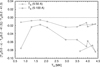 |
Fig. A.1 The differences of the Tx values as computed by Eq. (1) for the two selected band widths (legend) relative to the one used in this work (6.2–41.3 Å), assuming CIE. Symbols belong to the PN bubbles of the 0.696 M⊙ simulation. The evolution of Tx occurs from low to high values and back when the star fades (cf. Fig. 13). |
Figure A.1 shows that the differences to the band width used in the present work 6.2–11.3 Å (0.3-2 keV) depend primarily on the low-energy limit. This is so since below 5 Å (2.5 keV) there is hardly any X-ray emission, even for the hotter bubbles. The closest agreements between the various Tx values of the three band widths appear around Tx ≈ 1.7 MK. At these temperatures most of the bubble’s emission occurs just within 10–50 Å (0.25–1.26 keV). In general, the band-width dependence of Tx is quite modest and is not exceeding 10% in the worst case. The X-ray band used in the literature (which is dictated by the existing X-ray space observatories) is obviously sufficient to provide a useful temperature estimate of the X-ray emitting bubbles of planetary nebulae.
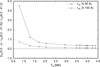 |
Fig. A.2 The difference of the Lx values based on the two selected band widths (legend) relative to the one used in this work (6.2–41.3Å), assuming CIE. Symbols belong to the same PN bubbles as Fig. A.1. |
Contrary to the bubble temperature, the corresponding X-ray luminosity is severely dependent on the chosen band width. This is demonstrated in Fig. A.2 where the Lx differences of the same bubbles as in Fig. A.1 are displayed. As expected, the luminosity differences increase with decreasing low-energy limit to very high values for cool bubbles. Any observed Lx value without indication of the used energy band is therefore useless.
Appendix B Comparison of the properties of different post-AGB evolutionary sequences
The existing hydrodynamical simulations of planetary-nebula evolution employ the evolutionary models available at the time, i.e. either those of Schönberner (1979, 1983) and Blöcker (1995) (used in the present work) or those of Vassiliadis & Wood (1993, 1994) (used by, e.g. Toalá & Arthur 2014, 2016). Both sets of models are based on the same or very similar physical assumptions with respect to radiative opacities and treatment of convection without overshoot.
The question now arises whether these hydrodynamical simulations are still of relevance in view of more recent post-AGB evolutionary calculations like those of Miller Bertolami & Althaus (2006) with the latest radiative opacities and inclusion of convective overshoot across radiative-convective boundary layers. Similar calculations have been performed by Weiss & Ferguson (2009), but they are not useful for our purposes because of the limited mass coverage. Miller Bertolami (2019) presented an extensive overview of the differences between the old and new evolutionary calculation with respect to the post-AGB phase. We concentrate here on the parameters that are of relevance for the hydrodynamical simulations, i.e. the luminosities of the AGB remnants and their timescales for crossing the HRD.
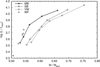 |
Fig. B.1 Luminosity of AGB remnants at Teff ≈ 30 000 K over remnant mass for the evolutionary calculations considered here: Miller Bertolami & Althaus (MB), Schönberner/Blöcker (SB), Vassiliadis & Wood (VW), and Weiss & Ferguson (WF). |
Figure B.1 shows a comparison of the luminosities of the AGB remnants when they enter the planetary nebulae region, i.e. at Teff ≈ 30 000 K (core-mass luminosity relation) from four different sets of evolutionary calculations. We see a large discrepancy between the older and newer calculations, in the sense that the new models have higher luminosities for given remnant masses.8
The rather high dependence of the post-AGB luminosity on the physics employed is of paramount importance because the bolometric luminosity is the only possibility for estimating an AGB remnant’s mass via evolutionary calculations. For given luminosity, we find from Fig. B.1 a mass difference of 0.03 …0.05 M⊙ between the Schönberner/Blöcker and Miller Bertolami mass scale. Therefore, it is absolutely mandatory to indicate the source of the post-AGB tracks used for any mass estimation.
The differences of the post-AGB luminosities translate directly into the differences of the crossing times from Teff = 10 000 K to maximum stellar temperature, as one can clearly see in Fig. B.2. This difference is considerable: the Miller Bertolami models evolve faster than the Schönberner/Blöcker models by factors between four and six.
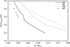 |
Fig. B.2 Crossing time, tcross, of AGB remnants from Teff = 10 000 K to maximum stellar temperature for the same models as in Fig. B.1, adapted from Fig. 1 of Miller Bertolami (2019). Differences caused by the metallicity are small and not relevant here. |
The smooth decrease of tCross with mass is distorted around 0.58 M⊙ (Miller Bertolami & Althaus 2006) or 0.62 M⊙ (Blöcker 1995). This distortion is the signature of the transition from initially ‘low mass’ to ‘intermediate-mass’ stars, i.e. from stars which ignite helium via a core flash to stars which ignite helium quiescently. Hence, the stars of these two groups start their AGB evolution with a different internal structure which in turn leads to an adjustment of the respective crossing times. A thorough discussion of the impact of the internal structure of an AGB star on the HRD crossing time can be found in Blöcker (1995).
Figure B.3 is a combination of the Figs. B.1 and B.2 and shows the relations between post-AGB masses of Schönberner/Blöcker (top) and Vassiliadis & Wood (bottom) to the Miller Bertolami ones, such that the two curves trace a sequence of common luminosity and crossing time, respectively. First of all, it is very gratifying that both the crossing time and the bolometric luminosity lead to virtually the same relation as long as MMB ≲ 0.58 M⊙ (or MSB ≲ 0.62 M⊙). Up to these mass limits, virtually constant offsets between the three post-AGB evolutionary calculations can be used.
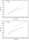 |
Fig. B.3 Relations between the masses of the Schönberner/Blöcker (top) and the Vassiliadis & Wood (bottom) post-AGB models against the Miller Bertolami post-AGB models along a common sequence of luminosity (Lbol) and crossing time (tcross), respectively. The dotted line is the 1:1 relation. |
This bevaviour is a consequence of (i) the fact that low-mass stars start their helium burning (by a core flash) at virtually the same core mass, independently of the total mass, and (ii) that a homologous core-envelope structures develop during the AGB phase of evolution.
This is not the case for intermediate-mass stars which begin helium burning quiescently in cores whose mass increases with total mass. Hence homologous structures cannot develop, and consequently a common scaling of masses based on luminosity and crossing time is not possible: above about 0.58 M⊙ (MB) both the luminosity and the crossing time give different relations between the Miller Bertolami and the Blöcker/Schönberner or Vassiliadis & Wood post-AGB masses (Fig. B.3). However, AGB remnants with such relatively high masses are not really important in the context of the present study because of their high luminosities (≳ 104 L⊙) and short crossing times (≲ 103 yr).
Numerically, the unique part of the relation between MMB ↔ MSB shown in Fig. B.3 (top) gives 0.535 ↔ 0.565 M⊙, 0.555 ↔ 0.595 M⊙, and 0.575 ↔ 0.625 M⊙. For higher remnant masses, the evolution of the two sets of models is truly different. While a MB model with 0.665 M⊙has the same post-AGB luminosity as a SB model with 0.696 M⊙, its HRD crossing time a about a factor of 2.5 shorter.
References
- Blöcker, T. 1995, A&A, 299, 755 [Google Scholar]
- Borkowski, K. J., Balbus, S. A., & Fristrom, C. C. 1990, ApJ, 355, 501 [NASA ADS] [CrossRef] [Google Scholar]
- Cahn, J. B., Kaler, J. B., & Stanghellini, L. 1992, A&AS, 94, 399 [Google Scholar]
- Cox, D. P., & Tucker, W. H. 1969, ApJ, 157, 1157 [Google Scholar]
- Crowther, P. A., Morris, P. W., & Smith, J. D. 2006, ApJ, 636, 1033 [NASA ADS] [CrossRef] [Google Scholar]
- de Freitas Pacheco, J. A., Costa, R. D. D., de Araújo, F. X., & Petrini, D. 1993, MNRAS, 260, 401 [NASA ADS] [CrossRef] [Google Scholar]
- Dere, K. P., Landi, E., Mason, H. E., Monsignori Fossi, B. C., & Young, P. R. 1997, A&AS, 125, 149 [NASA ADS] [CrossRef] [EDP Sciences] [Google Scholar]
- Dere, K. P., Landi, E., Young, P. R., et al. 2009, A&A, 498, 915 [NASA ADS] [CrossRef] [EDP Sciences] [Google Scholar]
- Dwarkadas, V. V. 2023, Galaxy, 11, 78 [NASA ADS] [CrossRef] [Google Scholar]
- Freeman, M. J., & Kastner, J. H. 2016, ApJS, 226, 15 [NASA ADS] [CrossRef] [Google Scholar]
- Freeman, M., Montez, R., Jr., Kastner, J. H., et al. 2014, ApJ, 794, 99 [NASA ADS] [CrossRef] [Google Scholar]
- Frew, D.J., Parker, Q. A., & BojiciC, I. S. 2016, MNRAS, 455, 1459 [Google Scholar]
- Georgiev, L. N., Peimbert, M., Hillier, D. J., et al. 2008, ApJ, 681, 333 [NASA ADS] [CrossRef] [Google Scholar]
- Girard, P., Köppen, J., & Acker, A. 2007, A&A, 463, 265 [NASA ADS] [CrossRef] [EDP Sciences] [Google Scholar]
- Gonzáles-Santamaría, I., Manteiga, M., Manchado, A., Ulla, A., & Dafonte, C. 2019, A&A, 630, A150 [NASA ADS] [CrossRef] [EDP Sciences] [Google Scholar]
- Górny, S. K., & Stasinska, G. 1995, A&A, 303, 893 [NASA ADS] [Google Scholar]
- Gruendl, R. A., Guerrero, M. A., Chu, Y.-H., & Williams, R. M. 2006, ApJ, 653, 339 [NASA ADS] [CrossRef] [Google Scholar]
- Guerrero, M. A., Chu, Y.-H., Gruendl, R. A., & Meixner, M. 2005, A&A, 430, L69 [NASA ADS] [CrossRef] [EDP Sciences] [Google Scholar]
- Guerrero, M. A., Ruiz, N., Hamann, W.-R., et al. 2012, ApJ, 755, 129 [NASA ADS] [CrossRef] [Google Scholar]
- Hamann, W.-R. 1997, IAU Symp. 180, 91 [NASA ADS] [Google Scholar]
- Heller, R., Jacob, R., Steffen, M., Schönberner, D., & Sandin, C. 2018, A&A, 620, A98 (Paper II) [NASA ADS] [CrossRef] [EDP Sciences] [Google Scholar]
- Herald, J. E., & Bianchi, L. 2004, ApJ, 611, 294 [NASA ADS] [CrossRef] [Google Scholar]
- Herald, J. E., & Bianchi, L. 2007, ApJ, 661, 845 [NASA ADS] [CrossRef] [Google Scholar]
- Herald, J. E., & Bianchi, L. 2011, MNRAS, 417, 2440 [NASA ADS] [CrossRef] [Google Scholar]
- Hillier, D. J., & Miller, D. L. 1999, ApJ, 519, 354 [Google Scholar]
- Kahn, F. D., & Breitschwerdt, D. 1990, MNRAS, 242, 505 [NASA ADS] [CrossRef] [Google Scholar]
- Kastner, J. H., Montez, R., Jr., Balick, B., De Marco, O. 2008, ApJ, 672, 957 [NASA ADS] [CrossRef] [Google Scholar]
- Kastner, J. H., Montez, R., Jr., Balick, B., et al. 2012, AJ, 144, 58 [NASA ADS] [CrossRef] [Google Scholar]
- Keller, G. R., Bianchi, L., & Maciel, W. J. 2014, MNRAS, 442, 1379 [NASA ADS] [CrossRef] [Google Scholar]
- Koo, B.-C., & McKee, C. F. 1992a, ApJ, 338, 93 [NASA ADS] [CrossRef] [Google Scholar]
- Koo, B.-C., & McKee, C. F. 1992b, ApJ, 338, 103 [NASA ADS] [CrossRef] [Google Scholar]
- Kudritzki, R.P., Urbaneja, M.A., & Puls, J. 2006, IAU Symp., 234, 119 [CrossRef] [Google Scholar]
- Leuenhagen, U., Hamann, W.-R., & Jefferey, C. S. 1996, A&A, 312, 167 [NASA ADS] [Google Scholar]
- Liedahl, D. A. 1999, Lect. Notes Phys., 520, 189 [NASA ADS] [CrossRef] [Google Scholar]
- Lindegren, L., Hernández, Bornbrun, A, et al. 2018, A&A, 616, A2 [NASA ADS] [CrossRef] [EDP Sciences] [Google Scholar]
- Marcolino, W. L. F., Hillier, D. J., de Araujo, F. X., & Pereira, C. B. 2007, ApJ, 654, 1068 [NASA ADS] [CrossRef] [Google Scholar]
- Marten, H., & Szczerba, R. 1997, A&A, 325, 1132 [NASA ADS] [Google Scholar]
- Mellema, G. 1998, Ap&SS, 260, 203 [Google Scholar]
- Mellema, G., & Lundqvist, P. 2002, A&A, 394, 901 [NASA ADS] [CrossRef] [EDP Sciences] [Google Scholar]
- Méndez, R. H., Kudritzki, R. P., & Herrero, A. 1992, A&A, 260, 329 [NASA ADS] [Google Scholar]
- Mewe, R. 1999, Lect. Notes Phys., 520, 109 [NASA ADS] [CrossRef] [Google Scholar]
- Miller Bertolami, M. M. 2019, Proc. IAU Symp., 343, 36 [Google Scholar]
- Miller Bertolami, M. M., & Althaus, L. G. 2006, A&A, 454, 845 [NASA ADS] [CrossRef] [EDP Sciences] [Google Scholar]
- Morisset, C., & Georgiev, L. 2009, A&A, 507, 1517 [NASA ADS] [CrossRef] [EDP Sciences] [Google Scholar]
- Pauldrach, A., Puls, J., Kudritzki, R.-P., Méndez, R. H., & Heap, S. R. 1988, A&A, 207, 123 [NASA ADS] [Google Scholar]
- Pauldrach, A. W. A., Hoffmann, T. L., & Méndez, R. H. 2004, A&A, 419, 1111 [NASA ADS] [CrossRef] [EDP Sciences] [Google Scholar]
- Perinotto, M., Kifonidis, K., Schönberner, D., & Marten, H. 1998, A&A, 332, 1044 [NASA ADS] [Google Scholar]
- Perinotto, M., Schönberner, D., Steffen, M., & Calonaci, C. 2004, A&A, 414, 993 [NASA ADS] [CrossRef] [EDP Sciences] [Google Scholar]
- Reimers, D. 1975, in Problems in Stellar Atmospheres and Envelopes, eds. B. Baschek, W. H. Kegel, & G. Traving (Berlin: Springer), 229 [CrossRef] [Google Scholar]
- Ruiz, N., Chu, Y.-H., Gruendl, R. A., et al. 2013, ApJ, 767, 35 [NASA ADS] [CrossRef] [Google Scholar]
- Sandin, C., Steffen, M., Schönberner, D., Rühling, U., & Hamann, W. R. 2011, Asymmetric Planetary Nebulae 5 Conf., eds. A. A. Zijlstra, F. Lykou, I. McDonald, & E. Lagadec, Jodrell Bank Centre for Astrophysics, A53 [Google Scholar]
- Sandin, C., Steffen, M., Schönberner, D., & Rühling, U. 2016, A&A, 586, A57 (Paper I) [NASA ADS] [CrossRef] [EDP Sciences] [Google Scholar]
- Schönberner, D. 1979, A&A, 79, 108 [Google Scholar]
- Schönberner, D. 1983, ApJ, 272, 708 [NASA ADS] [CrossRef] [Google Scholar]
- Schönberner, D., & Blöcker, T. 1993, ASP Conf. Ser., 45, 337 [Google Scholar]
- Schönberner, D., Jacob, R., Lehmann, H., et al. 2014, Astron. Nachr., 335, 378 [CrossRef] [Google Scholar]
- Schönberner, D., Balick, B. & Jacob, R. 2018, A&A, 609, A126 [NASA ADS] [CrossRef] [EDP Sciences] [Google Scholar]
- Soker, N. 1994, AJ, 107, 276 [CrossRef] [Google Scholar]
- Solf, J., & Weinberger, R. 1984, A&A, 130, 269 [NASA ADS] [Google Scholar]
- Steffen, M., Schönberner, D., & Warmuth, A. 2008, A&A, 489, 173 [NASA ADS] [CrossRef] [EDP Sciences] [Google Scholar]
- Steffen, M., Sandin, C., Jacob, R., & Schönberner, D. 2012, IAU Symp., 283, 215 [NASA ADS] [Google Scholar]
- Steffen, M., Hubrig, S., Todt, H., et al. 2014, A&A, 570, A88 [NASA ADS] [CrossRef] [EDP Sciences] [Google Scholar]
- Stute, M., & Sahai, R. 2006, ApJ, 651, 882 [NASA ADS] [CrossRef] [Google Scholar]
- Toalá, J. A., & Arthur, S. J. 2014, MNRAS, 443, 3486 [CrossRef] [Google Scholar]
- Toalá, J. A., & Arthur, S. J. 2016, MNRAS, 463, 4438 [CrossRef] [Google Scholar]
- Toalá, J. A., & Arthur, S. J. 2017, MNRAS, 464, 178 [CrossRef] [Google Scholar]
- Toalá, J. A., & Arthur, S. J. 2018, MNRAS, 478, 1218 [CrossRef] [Google Scholar]
- Toalá, J. A., Guerrero, M. A., Todt, H., et al. 2015, ApJ, 799, 67 [Google Scholar]
- Toalá, J. A., Montez Jr. R., & Karovska, M. 2019a, ApJ, 886, 30 [CrossRef] [Google Scholar]
- Toalá, J. A., Ramos-Larios, G., Guerrero, M. A., & Todt, H. 2019b, MNRAS, 485, 3360 [Google Scholar]
- Toalá, J. A., Guerrero, M. A., Bianchi, L., Chu, Y.-H., & De Marco, O. 2020, MNRAS, 494, 3784 [CrossRef] [Google Scholar]
- Todt, H., Kniazev, A. Y., Gvaramadze, V. V., et al. 2015, ASP Conf. Ser., 493, 539 [NASA ADS] [Google Scholar]
- Vassiliadis, E., & Wood, P. R. 1993, ApJ, 413, 641 [Google Scholar]
- Vassiliadis, E., & Wood, P. R. 1994, ApJS, 92, 125 [NASA ADS] [CrossRef] [Google Scholar]
- Villaver, E., Manchado, A., & García-Segura, G. 2020, ApJ, 581, 1204 [Google Scholar]
- Weaver, R., McCray, R., Castor, J., Shapiro, P., & Moore, R. 1977, ApJ, 218, 377 [Google Scholar]
- Weiss, A, & Ferguson, J. W. 2009, A&A, 508, 1343 [NASA ADS] [CrossRef] [EDP Sciences] [Google Scholar]
- Yu, Y. S., Nordon, R., Kastner, J. H., et al. 2009, ApJ, 690, 440 [NASA ADS] [CrossRef] [Google Scholar]
- Zhekov, S. A. 2014, MNRAS, 443, 12 [CrossRef] [Google Scholar]
- Zhekov, S. A., & Park, S. 2011, ApJ, 728, 135 [NASA ADS] [CrossRef] [Google Scholar]
- Zhekov, S. A., & Perinotto, M. 1996, A&A, 309, 648 [NASA ADS] [Google Scholar]
We note that both the simulations of Stute & Sahai (2006) and Toalá & Arthur (2014) only allow the development of 2D structures in spherical coordinates.
The time needed for a wind parcel to reach the wind shock.
We use the measured parallaxes, π, without the (very small) zero point corrections to compute distances as d = 1 /π.
Kastner et al. (2008) used higher bubble radii taken from the catalogue of Cahn et al. (1992). However, this catalogue only lists the outer nebular radii!
Valid only initially; once ionisation sets in, the density ahead of R2 will no longer follow a simple ρ ∝ r−2 law.
The crossing time is the time needed by an AGB remnant to evolve from the tip of the AGB to maximum effective temperature (see, e.g. Blöcker 1995).
The true (clumpy) mass loss rate is relevant for heating the bubble, even though our models assume a homogeneous wind (but see also Sect. 7.3).
We note that the remnant luminosity depends not only on the remnant mass but also somewhat on the thermal-pulse cycle phase when the star leaves the tip of the AGB, which can differ from sequence to sequence.
All Tables
Chemical composition of the stellar wind (WR) and the nebular gas (PN) used for computing the hydrodynamical models and synthetic X-ray spectra in terms of mass fractions (Cols. 3 and 5) and (logarithmic) number fractions ϵ (Cols. 4 and 6), arranged by atomic number Z.
Compilation of stellar and X-ray properties of the objects discussed in this paper.
All Figures
|
Fig. 1 Evolution of stellar parameters and wind properties of our standard model of a 0.595 M⊙ AGB remnant. Left column: Run of stellar bolometric, Lstar/L⊙ (top), and wind luminosity, |
| In the text | |
|
Fig. 2 Positions of hot-bubble formation in a Teff-R2 diagram for three different ‘families’ of the simulations from Table 2 (see legend). The numbers along the symbols are the usual mass-loss rate factors of the simulations, while the tilted numbers indicate the wind velocity (in km s−1) at the moment of hot-bubble formation. The dotted lines connect members of the same family. |
| In the text | |
|
Fig. 3 Evolution of different parts of the bubble mass with stellar temperature Teff for the simulations WR100V05 and WR100V05x5.5. The total X-ray-emitting bubble mass is MX = MWR + MPN, where MWR is the mass contributed by the stellar wind and MPN that of the evaporated nebular matter. The symbols mark the models for which the data were evaluated. The evolution of MX(PN1) of the hydrogen-rich PN1 reference simulation is shown for comparison (asterisks). The three bubble models of the WR100V05 simulation whose temperature profiles are displayed in Fig. 4 are marked along the top abscissa. |
| In the text | |
|
Fig. 4 Radial temperature profiles of three typical bubbles of the WR100V05 simulation. From top to bottom, the models represent case 1 (Teff = 44 000 K), case 2 (Teff = 56 000 K), and case 3 (Teff = 80 000 K, with beginning evaporation). The central star is at r = 0 cm. The vertical dashed lines mark the transition from the hydrogen-poor WR (left) to the hydrogen-rich PN chemistry (right). The bubble parameters like characteristic X-ray-temperatures, X-ray luminosities, and masses (for the entire bubble and for the respective subregions with the WR or PN composition) are given in the legends. The symbols on the bubble’s temperature profile mark different characteristic temperatures: of the entire bubble (diamond), the hydrogen-poor part only (star), and the hydrogen-rich evaporated part only (plus). |
| In the text | |
|
Fig. 5 Ionisation structure of the WR100V05 model displayed in Fig. 6. The upper panels show the radial profiles of the NEI ionisation fractions for the last four ionisation stages of carbon (left), oxygen (middle), and neon (right) as computed with NEBEL/CORONA. The NEI to CIE logarithmic number density ratios are plotted in the respective bottom panels. The wind shock is at R1 = 2.5 × 1017 cm, the bubble’s surface (conduction front) at R2 = 6.5 × 1017 cm. |
| In the text | |
|
Fig. 6 Hot-bubble structure of the WR100V05 simulation at t = 9107 yr, Teff = 139 968 K, L⋆ = 2841 L⊙· Top: radial profile of electron temperature (dashed, right ordinate), electron density (dotted), and ion density (solid). The star is at r = 0, the wind’s reverse shock at R1 = 2.5 × 1017 cm. The transition from the wind-shocked hydrogen-poor WR matter to the evaporated nebular PN matter is at r = 4.6 ×1017 cm (T ≃ 5.0 MK), the heat conduction front (bubble-nebula interface) at R2 = 6.5 ×1017 cm, and the high-density region between 6.5 × 10¹⁷ and 8.3 × 1017 cm is the fully ionised planetary nebula proper with its double-shell structure and an electron temperature of about 1.2×10⁴ K. Middle: X-ray surface brightness distribution (6–11 Å) for the same model, assuming CIE, before (solid) and after (dashed) absorption by a hydrogen column density of NH = 0.25 × 1022 cm−2. The masses contained in the two bubble parts are 3.05 ×10⁻³ M⊙ of WR matter, supplied by the stellar wind, and 4.24 ×10⁻³ M⊙ of evaporated PN matter. Bottom: same as middle panel, but assuming NEI of nine key elements. |
| In the text | |
|
Fig. 7 Evolution of stellar energy output of four AGB models with remnant masses of 0.565, 0.595, 0.625, and 0.696 M⊙ (already used in SSW and Ruiz et al. 2013) versus their effective temperatures. The ‘reference’ track of Fig. 1, 0.595 M⊙, is highlighted by a thick red line. The positions of the objects from Table 3 are labelled with the object’s number within either a circle (O-type central star) or a hexagon ([WR]-type central star). Top: stellar bolometric photon luminosity; NGC 7026 (no. 12) falls outside the plotted luminosity range. Bottom: wind luminosity of the same AGB-remnants; NGC 7026 is now included. Solid tracks refer to the ‘standard’ mass-loss model ṀPPKMH (Pauldrach et al. 1988, see Sect. 2). The dashed track corresponds to a 0.595 M⊙ model with the wind power increased by a factor of 50 (see text). |
| In the text | |
|
Fig. 8 Stellar-wind velocities (top) and mass-loss rates (bottom) versus stellar Teff for the same post-AGB tracks and sample objects as in Fig. 7. The dash-dotted line in the top panel represents the wind velocity of the 0.595 M⊙ model halved, the dashed line in the bottom panel the mass-loss rate of the 0.595 M⊙ model increased by a factor of 200. The positions of the objects no. 6 (NGC 3242) and no. 8 (NGC 5315) nearly coincide in the top panel, and those of no. 5 (NGC 2392) and no. 10 (NGC 6826) in the bottom panel. |
| In the text | |
|
Fig. 9 Bubble radius, log(R2) versus central-star effective temperature, Teff, as predicted by our hydrodynamical simulations of the 0.565, 0.595 (PN), 0.625, and 0.696 M⊙ sequences together with the sample objects. The dashed line refers to that in Fig. 7 (bottom panel) and is an estimate based on Eq. (5) if the wind power of the 0.595 M⊙ model is increased by a factor of 50. The simulations are plotted from the beginning of bubble formation till maximum stellar temperature. |
| In the text | |
|
Fig. 10 X-ray HRD for our sample objects of Table 3 (symbols as in previous figures) together with the predictions of heat-conducting hydrodynamical bubble models around the 0.565, 0.595, 0.625, and 0.696 M⊙ sequences. The symbols (squares) along the sequences denote the individual models for which the X-ray emission has been computed by means of the CHIANTI software package. The top panel shows the NEI, the bottom panel the CIE case. |
| In the text | |
|
Fig. 11 Same as in Fig. 10, but for the characteristic bubble temperature Tx. The objects with very uncertain Tx values are shown in grey (Tx entries of Table 3 in italics). |
| In the text | |
|
Fig. 12 X-ray luminosity versus bubble size of the sample objects listed in Table 3 (numbered symbols) together with the predictions of the four hydrogen-rich bubble sequences of the previous figures. Again, the NEI and CIE case is shown at top and bottom, respectively. |
| In the text | |
|
Fig. 13 Same as in Fig. 12, but for the characteristic bubble temperature Tx. The objects with very uncertain Tx values are shown in grey (Tx entries of Table 3 in italics). |
| In the text | |
|
Fig. 14 Same as in Fig. 9 but now only for the new hydrogen-poor bubble sequences WR100V05 (upper) and WR100V05x5.5 (lower) together with the bubbles of the [WR] objects in Table 3. The black crosses indicate the moments of hot-bubble formation (big crosses) and the start of evaporation (small crosses). |
| In the text | |
|
Fig. 15 Bubble X-ray luminosities Lx versus bubble radius R2 of the sequences WR100V05 (right, solid) and WR100V05x5.5 (left, dashed) and the bubbles of the [WR]-type sample objects of Table 3. Evolution occurs from left to right, and maximum stellar temperatures are indicated by a vertical mark. Evaporating bubble models are connected by a thick solid or dashed line. The WR100V05 bubbles also contain the information on the luminosity contributions of the hydrogen-poor WR part (crosses) and the evaporated hydrogen-rich PN part (triangles). The arrow indicates the (estimated) shift of the WR100V05 bubbles if the evolutionary timescale is increased by a factor of 2.5. The top panel displays the NEI, the bottom panel the CIE case. |
| In the text | |
|
Fig. 16 Characteristic X-ray temperature TX versus bubble radius R2 for the sequences WR100V05 (right, solid) and WR100V05x5.5 (left, dashed) and the bubbles of our sample (Table 3). Again, bubble evolution occurs from left to right, and maximum stellar temperatures are indicated by a vertical mark. Evaporating bubbles with inhomogeneous composition are connected by thick solid or dashed lines. The mean temperatures of the hydrogen-poor part, TX(WR), and of the hydrogen-rich part, TX(PN), are shown as crosses and triangles, respectively, for the WR100V05 bubbles. As in the previous figure, the arrow indicates the (estimated) shift of the WR100V05 bubbles if the evolutionary timescale is increased by a factor of 2.5. The symbol of NGC 40 (no. 4) is shown in grey because of the large uncertainty of the derived TX value. The top and bottom panel displays the NEI and the CIE case, respectively. |
| In the text | |
|
Fig. A.1 The differences of the Tx values as computed by Eq. (1) for the two selected band widths (legend) relative to the one used in this work (6.2–41.3 Å), assuming CIE. Symbols belong to the PN bubbles of the 0.696 M⊙ simulation. The evolution of Tx occurs from low to high values and back when the star fades (cf. Fig. 13). |
| In the text | |
|
Fig. A.2 The difference of the Lx values based on the two selected band widths (legend) relative to the one used in this work (6.2–41.3Å), assuming CIE. Symbols belong to the same PN bubbles as Fig. A.1. |
| In the text | |
|
Fig. B.1 Luminosity of AGB remnants at Teff ≈ 30 000 K over remnant mass for the evolutionary calculations considered here: Miller Bertolami & Althaus (MB), Schönberner/Blöcker (SB), Vassiliadis & Wood (VW), and Weiss & Ferguson (WF). |
| In the text | |
|
Fig. B.2 Crossing time, tcross, of AGB remnants from Teff = 10 000 K to maximum stellar temperature for the same models as in Fig. B.1, adapted from Fig. 1 of Miller Bertolami (2019). Differences caused by the metallicity are small and not relevant here. |
| In the text | |
|
Fig. B.3 Relations between the masses of the Schönberner/Blöcker (top) and the Vassiliadis & Wood (bottom) post-AGB models against the Miller Bertolami post-AGB models along a common sequence of luminosity (Lbol) and crossing time (tcross), respectively. The dotted line is the 1:1 relation. |
| In the text | |
Current usage metrics show cumulative count of Article Views (full-text article views including HTML views, PDF and ePub downloads, according to the available data) and Abstracts Views on Vision4Press platform.
Data correspond to usage on the plateform after 2015. The current usage metrics is available 48-96 hours after online publication and is updated daily on week days.
Initial download of the metrics may take a while.