| Issue |
A&A
Volume 618, October 2018
|
|
|---|---|---|
| Article Number | A17 | |
| Number of page(s) | 46 | |
| Section | Stellar structure and evolution | |
| DOI | https://doi.org/10.1051/0004-6361/201833484 | |
| Published online | 05 October 2018 | |
How common is LBV S Doradus variability at low metallicity?⋆,⋆⋆
1 Departamento de Astronomía, Universidad de Chile, Casilla 36-D, Santiago, Chile
e-mail: This email address is being protected from spambots. You need JavaScript enabled to view it.
2 Armagh Observatory, College Hill, BT61 9DG Armagh, UK
3 Astrophysics Research Centre, School of Mathematics and Physics, Queen’s University Belfast, BT7 1NN, Belfast, UK
4 School of Physics, O’Brien Centre for Science North, University College Dublin, Belfield, Dublin 4, Ireland
Received:
23
May
2018
Accepted:
21
June
2018
Abstract
It remains unclear whether massive star evolution is facilitated by mass loss through stellar winds only or whether episodic mass loss during an eruptive luminous blue variable (LBV) phase is also significant. LBVs exhibit unique photometric and spectroscopic variability (termed S Doradus variables). This may have tremendous implications for our understanding of the first stars, gravitational wave events, and supernovae. A key question here is whether all evolved massive stars passing through the blue supergiant phase are dormant S Doradus variables transforming during a brief period or whether LBVs are truly unique objects. By investigating the OGLE light curves of 64 B supergiants (Bsgs) in the Small Magellanic Cloud (SMC) on a timescale of three years with a cadence of one night, the incidence of S Doradus variables amongst the Bsgs population is investigated. From our sample, we find just one Bsg, AzV 261, that displays the photometric behaviour characteristic of S Doradus variables. We obtain and study a new VLT X-shooter spectrum of AzV 261 in order to investigate whether the object has changed its effective temperature over the last decade. We do not find any effective temperature variations indicating that the object is unlikely to be a LBV S Doradus variable. As there is only one previous bona fide S Doradus variable known to be present in the SMC (R 40), we find the maximum duration of the LBV phase in the SMC to be at most a few 103 yr or more likely that canonical Bsgs, and S Doradus LBVs are intrinsically different objects. We discuss the implications for massive star evolution in low-metallicity environments, characteristic of the early Universe.
Key words: stars: variables: S Doradus / stars: evolution / Magellanic Clouds
Based on observations collected at the European Organisation for Astronomical Research in the Southern Hemisphere under ESO programme 299.D-5054(A).
The full Table 1 is only available at the CDS via anonymous ftp to cdsarc.u-strasbg.fr (130.79.128.5) or via http://cdsarc.u-strasbg.fr/viz-bin/qcat?J/A+A/618/A17
© ESO 2018
1. Introduction
Massive stars are important producers of radiative and kinetic energy in the Milky Way, whilst massive stars in low-metallicity environments may provide us with key insights into their ionizing input in the early Universe. However, the evolution and fate of the most massive stars in the Universe, especially at low metal content, is highly uncertain (Langer 2012). A key question is whether the bulk of the mass is lost either in stellar winds (Chiosi & Maeder 1986), in luminous blue variable (LBV) type eruptions, or binary interactions (Smith & Tombleson 2015), and how mass loss varies with metal content (Vink et al. 2001; Puls et al. 2008).
If low-metallicity massive stars indeed lose substantial amounts of mass in the LBV phase, this could be pivotal for our understanding of pristine Pop III stars (Vink & de Koter 2005; Smith & Owocki 2006), as it is usually assumed that these objects keep their initial masses intact (Woosley & Heger 2015). The mass-loss process at low metallicity is key for understanding seed black hole masses in the early Universe, the “heavy” black holes recently identified from the gravitational wave event GW 150914 (Abbott et al. 2016), and supernovae and supernovae impostors at low metallicity (Trundle et al. 2008).
Physically, LBVs can be understood as variables within the evolved massive blue supergiant zoo. B supergiants (Bsgs) are evolved massive stars (>15 M⊙) which are thought to be in a transitional stage from the main sequence towards the evolved Wolf–Rayet stage (although as noted in Vink et al. 2010 it is unclear whether Bsgs are hydrogen-burning main sequence stars with a large overshooting parameter, or helium-core burning stars). Most Bsgs display intrinsic photometric variability that are characterized by their amplitude and timescales as one of three types:
α-Cyg variables, which display (likely periodic) micro-variations of ≲0.1m on timescales from days to months, now commonly thought to be due to non-radial gravity mode pulsations (Lefever et al. 2007);
S Doradus variables (or luminous blue variables; LBVs), which display aperiodic variations of ≳0.1m (van Genderen 2001) on timescales from years to decades encompassing a wide variety of light curves in amplitude and time, with a clear distinction made in colour-brightness changes. Although no commonly accepted paradigm exists for the cause of the variability it must consist of radius inflation to explain the observed changes in optical brightness and spectral type, rather than dust obscuration events. Almost all S Doradus variables also display α-Cyg variations, whilst the opposite is not the case;
η Car variables (or eruptive LBVs; or supernova impostors), which show changes of >1–2m within days indicative of an eruptive event. These events are extremely rare (around one per century in our Galaxy), with the most famous example being η Car (de Vaucouleurs & Eggen 1952).
Classically, most S Doradus variables have been found serendipitously either through identification of their peculiar variability (Humphreys et al. 2016), or more recently, from their compact shells by infrared imaging (Gvaramadze et al. 2012). LBVs are rare; ∼20 bona fide LBVs are currently known in the Milky Way and the 1/2 Z⊙ Large Magellanic Cloud (LMC), and only one bona fide member, R 40, is known in the 1/5 Z⊙ Small Magellanic Cloud (SMC). It is not clear, however, whether the SMC star HD 5980 is an LBV or a Wolf–Rayet star (Humphreys et al. 2016; Smith & Tombleson 2015; Vink 2012; Humphreys & Davidson 1994).
Additionally, while it is thought that α-Cyg variables form a large fraction (if not most) of all Bsgs (Lefever et al. 2007), it remains unclear how common S Doradus and eruptive LBV variability are among Bsgs. In other words, do all Bsgs display S Doradus variability, albeit at smaller amplitudes or varying baselines?
For many decades given their extreme rarity (even for massive stars), LBVs were thought to represent a brief evolutionary phase (∼104 yr; Lamers et al. 1998) during a massive star’s life between the hydrogen-burning main sequence, and the core helium burning Wolf–Rayet phase. As LBVs lie close to the Humphreys–Davidson instability limit (Humphreys & Davidson 1994), they are linked to an instability which allows massive stars to lose mass, preventing them from becoming red supergiants (RSGs). Within this period of extreme mass loss the brightness increases in line with an inflation of the envelope, resulting in a temperature decrease (Gräfener et al. 2012; Vink 2015). This picture is corroborated by their light curves, which show S Dor-type decadal variations (0.5–2 mag) interspersed by micro-variations (of the order of 0.1–0.2 mag).
Although, it has traditionally been suggested that S Doradus LBVs are transitional objects (Humphreys & Davidson 1994; Lamers et al. 1998), in the last decade, they have been proposed as direct core-collapse supernovae SNe progenitors (Kotak & Vink 2006; Gal-Yam & Leonard 2009; Groh et al. 2013; Smith 2014). Additionally, searches for LBVs in nearby galaxies (e.g. Massey et al. 2007) have found a vast number of LBV candidates without the distinctive photometric variability, and have suggested that there are large number of Bsgs that are not eruptive LBVs but probably dormant S Doradus LBV variables. This would suggest a much longer lifetime for the LBV phase (∼105 yr), comprising a significant fraction of the He-burning phase. However, a number of the LBV candidates found by Massey et al. (2007) have been shown to be sgB[e] stars (a small subset of Bsgs whose evolutionary status remains unclear; see Miroshnichenko 2006). It has been suggested that sgB[e] and LBVs do not evolve into one another (see Humphreys et al. 2017b).
In order to properly unravel the evolutionary status of the LBVs at low metallicity, we need to increase the number of confirmed LBVs in low-metallicity galaxies. The key question is whether S Doradus LBVs are truly special Bsg objects, or if all Bsgs might actually be dormant LBVs. In the latter case the total number of LBVs might be an order of magnitude larger than the number of bona fide LBVs would suggest (see Massey et al. 2007) and hence their lifetimes would increase to 105 yr or more, with relevant consequences for their evolutionary state.
In this study, we present a systematic search for LBVs using long-baseline (3 yr) medium-cadence (nightly) light curves of known Bsgs in the 1/5 Z⊙ local group dwarf galaxy Small Magellanic Cloud (SMC). The data allow us to accurately quantify the incidence of S Doradus variability among known B Sgs. The main aim of the study is to quantify the incidence of S Doradus variability among the Bsgs population in order to establish whether most Bsgs are in fact dormant S Doradus LBVs or if S Doradus LBVs are intrinsically different to Bsgs.
This paper is organized as follows: Sect. 2 describes the analysis of the light curves of known B Sgs. Section 3 describes the identification of the sole potential S Doradus variable, AzV 261. Section 4 presents a discussion of the results. Our conclusions are given in Sect. 5.
2. Analysis of periodicity of B Sgs in the SMC
2.1. Bsgs sample
We selected Bsgs with multi-epoch photometric data obtained during the second phase of the OGLE II were selected for analysis. The OGLE II survey obtained multi-epoch I-band imaging of the SMC. The photometry covers a period of 3 yr spanning approximately from 1 June 1997 to 31 November 2000. at a cadence of approximately every night. The data cover only the periods (for approximately 8 months each year) across the baseline in which the SMC is visible from the Warsaw telescope situated at the Las Campanas Observatory in Chile. The median seeing of the imaging is around 1″, with a resulting median random photometric uncertainty of ∼0.007 mag. Bad data points are identified and removed according to the difference imaging criterion. The reader is referred to the OGLE II survey publication (Szymanski 2005; Udalski et al. 1997) for further details of the data.
The stellar classifications given by Bonanos et al. (2010) were used to compile a list of 179 known SMC Bsgs. In the case of multiple varying classifications, we chose the most recent classification based on spectroscopy. A cross-match with a tolerance of 1″ (the median seeing of the photometry) was performed with the OGLE II I-band imaging. Over the total field of view of the OGLE II survey, there are 110 known Bsgs, of which 69 Bsgs had multi-epoch I-band photometry (20 Bsgs had OGLE II photometry, but not light curves, while 21 did not have OGLE II photometry even though they fall within the OGLE II field of view). The recovered 69 Bsgs cover the entire B spectral type, and are split based on their luminosity classification into 16 BIa, 24 BIab, and 24 BIb Bsgs, and 5 with no luminosity classification. The five Bsgs without luminosity classification were discarded from the final catalogue. The total number of identified Bsgs, and the total known in the OGLE II survey area are shown as a fraction in Fig. 1 as a function of spectral type. The recovery fraction is ∼70% until spectral type B6. For binomial statistics, the recovered sample size can predict simple binomial properties at the 99% confidence level with a 10% margin of error. Although the selection criteria are unbiased, OGLE II photometry saturates around V ∼ 12. Our final sample is thus not uniformly distributed in either spectral type or brightness, but does contain a sufficiently representative sample of Bsgs for our analysis. A list of the Bsgs and their photometric properties is given in Table 1.
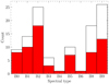 |
Fig. 1. Recovered spectral types of Bsgs in our sample (red) and the total number of Bsgs in the SMC (solid line) within the OGLE II survey area. |
Properties of Bsgs having photometry in the OGLE II survey.
2.2. Analysis of time series data
S Doradus variables present multiple types of photometric variability (van Genderen 2001), presumably due to an inflating radius and decreasing photospheric temperature. The photometric variability is between 0.1 (below which most micro-variations are generally caused by the α-Cyg ℊ-mode pulsations) and 2.5 mag (above which most variations are due to eruptive events, falling into the eruptive phase of LBVs) on timescales of years to decades. Light curves within this broad magnitude and time span show diverse characteristics, yet few distinctive features thus excluding them from most other variables.
Primarily, the light curve varies on timescales greater than a year (not considering α Cyg variations), with a systematic trend in brightness. Additionally, a decrease in brightness is accompanied by a bluer colour and vice versa. While the former rules out short period variability, the latter precludes variability due to dust obscuration events, and is considered a genuine increase in stellar radius. Considering the periodicity of S Doradus variables, there are multiple cycles/periodicities present in the light curve with pronounced beats, although overall the light curve increases/decreases aperiodically.
In this section, we search the light curves of the Bsgs to identify stars with multiple periodicities, and/or irregular photometric variability above 0.1m. To place this into context, we also compare our light curves with those of known S Doradus variables in the Magellanic Clouds. The light curves of the Bsgs are presented in Figs. 2 and A.1. We discuss our results below.
2.2.1. Searching for periodic variability
In Figs. 2 and A.1, we plot the light curves of 64 Bsgs and search for photometric variability at periodic and aperiodic timescales which may have been caused by outbursts. Identification of periodic variability is comparatively straightforward. To do so, we employed the Lomb–Scargle periodogram, which is a statistical tool often used to identify periodic variations in unevenly spaced observations. A power spectrum for each Bsg light curve was constructed. The period range was 0.5–1000 d, with a frequency grid spacing of 0.0037 d−1. The significance of the identified peaks was tested by a Monte Carlo simulation (see e.g. VanderPlas 2018; Frescura et al. 2007). To do so, 1000 simulated light curves were generated using a bootstrapping technique, where random data pairs are replaced from the original light curves. The bootstrapping technique gives us a significance level for the periods detected. Each Bsg showing a peak in the power spectrum greater than the 99% level can be identified as a periodic variable following the methods outlined in VanderPlas (2018), and shown in Figs. 3 and B.1.
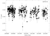 |
Fig. 2. Representative light curve of the Bsg 2dFS0153 from the OGLE survey, where the measured OGLE I-band magnitude is plotted against the Julian Date. Light curves of all 64 Bsgs in our sample are shown in Fig. A.1. |
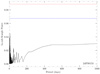 |
Fig. 3. Representative Lomb–Scargle periodogram of Bsg 2dFS0153. The period in days is plotted against the Lomb–Scargle power. The dashed red and blue lines are the 99% and 95% significance levels identified using the bootstrap Monte Carlo simulations. Periodic variables are those whose peak in the power spectrum is greater than the 99% significance level. Lomb–Scargle periodograms of the remaining 63 Bsgs are displayed in Fig. B.1. |
When searching for periodicity, we attempt to differentiate between short and intermediate period variables. Bsgs having short periodic variations (essentially with periods less than 2 days), are generally α Cyg variables (unless the amplitude of their variations exceeds a few tenths of magnitude). Nearly all Bsgs show periods of 1–2 days with varying amplitudes of 0.05–0.1 mag. However, given that our sampling frequency is about the same, we cannot conclusively identify such variations as being strictly periodic due to the star. We note that periodic variations around 0.5 and 1 d are in most cases almost certainly caused by sampling below the sampling frequency, representing the nightly half-cadence and cadence levels. Therefore, although in many cases multiple frequencies in this time regime are found, we cannot isolate them as being strictly stellar (and thereby α Cyg) with our data. Hence, any periodic variables below 1d are discarded from the final sample. In total, we identified five candidate periodic variable Bsgs in our sample. Split into groups based on luminosity class, 1 out 24 is BIabs, 1 out of 16 is BIas, and 3 out of 24 are BIbs. In all instances, the period is greater than the Nyquist frequency at the 3σ level (1% level, due to random variations). We did not attempt to smooth out any long term variability in the light curve. Only in the case of AzV 261 were multiple periods above the 3σ level found.
2.2.2. Searching for aperiodic variability
Searching for aperiodic variability is not straightforward compared to periodic variability as there are no commonly accepted metrics for massive stars (see e.g. Labadie-Bartz et al. 2017; Findeisen et al. 2015). We employed the δm–δt plots which are suggested by Mahabal et al. (2011) and Findeisen et al. (2015) as a better indicator of variability in a series of tests on simulated light curves, although the correlation with any period is low. The δm–δt plots are only used to identify variability, and further checks were done by eye as at times some features cannot be compared directly, as suggested by Labadie-Bartz et al. (2017).
The δm–δt plot presents the incidence of variability at a particular timescale in a light curve. It is defined as the sum of all observations at magnitude m and time t of a light curve, by computing the differences,
 (1)
(1)
and i > j such that each pair is only considered once. By presenting the differences between magnitude and time as a density histogram, we can directly observe how much variability is observed on what timescales (see Figs. 4 and C.1). We note that the δm–δt plot is closely related to the structure function used to characterize variability in galaxies. Overall, different timescales are sampled to varying levels in the plots; however, we are only interested in aperiodic/periodic variations greater than 0.1m on timescales greater than a few days. To aid in identification we compute the δm–δt plots of known S Doradus variables, R 40 and R 110, in the Magellanic Clouds1, and compare them with our Bsgs sample. From the δm–δt plots of the known S Doradus variables shown in Fig. 5, we identify only one BIb star as displaying aperiodic variability above the significance threshold: AzV 261.
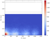 |
Fig. 4. Two-dimensional histogram (δm–δt) of the Bsg 2dFS1053 from the OGLE II data, where the colour gradient marks the density of the points (see the colourbar). The dashed line marks the 10σ level of the random photometric uncertainty, while the solid line differentiates variations above the 0.1m level. The δm–δt two-dimensional histograms of the remaining Bsgs are included in Fig. C.1. |
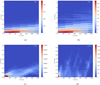 |
Fig. 5. Two-dimensional histogram (δm–δt) of known S Doradus variables R 40, R 110, S Doradus on (panel a), (panel b) and (panel c) respectively. The candidate S Doradus variable in our Bsgs sample, AzV 261 is shown in (panel d). Symbols are same as Fig. 4. |
3. AzV 261: a candidate S Doradus variable
Searching systematically through archival light curves from the OGLE database, we found that AzV 261 in the SMC is an excellent S Doradus candidate. In Fig. 6a, we show the I-band light curve of the star spanning a decade (1998–2009). The (V−I) colour behaviour is also shown (the additional time series data come from OGLE III data of Kourniotis et al. 2014). From Fig. 6, AzV 261 first displays micro-variations of ∼0.2 mag on timescales of days. In addition, the brightness increased by 0.53 mag from 13 November 2000 to 20 October 2008 (the OGLE-III data are until 2009). Using the Period04 software (Lenz & Breger 2005), we attempted to characterize further the periodicity and micro-variations. In the Lomb–Scargle periodogram, AzV 261 shows four significant peaks (see Fig. A.2 and Table 1). However, this light curve has a long-term trend of increasing brightness. We fit a fourth-order polynomial to remove this trend, and attempt using Period04 to fit periods to replicate the light curve of AzV 261. However, even with three periods, the residuals of the light curve are significant (see Fig. 6b) indicating that the observed possibly semi-periodic variations are micro-varitaions (see van Genderen 2001; Lamers et al. 1998). Based on its light curve, AzV 261 is the single likely LBV candidate in our sample.
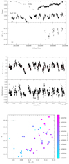 |
Fig. 6. Top: I-band light curve of AzV 261 spanning from 1998 to 2009. Also shown is the scaled historical light curve of the classic LBV star S Doradus for comparison (crosses). Panel b: (V−I) colour plotted against the Julian date for AzV 261. Middle: (panel a) light curve with the overall trend removed by a fourth-degree polynomial, with the best-fit predicted light curve (the three peaks are given in Table 1). Panel b: residuals between the fit period and the observed light curve. Bottom: V vs. (V−I) colour-magnitude diagram of AzV 261 over time, with time given by the colourbar. The behaviour of a brightness increase corresponding to a temperature decrease is seen here. |
In addition, the colour information from Fig. 6c strongly supports the LBV candidacy: the (V−I) colour becomes redder with time, corresponding to an actual temperature decrease. This is consistent with the picture of a brightness increase as the temperature decreases due to radius inflation, while the object’s bolometric luminosity stays roughly constant. Therefore, AzV 261 is a prime S Dor-type LBV candidate, the only one among 64 known Bsgs identified by our systematic search. Its light curve displays micro-variations of the order of 0.2 mag on timescales of a few days to months, with an overall increase over eight years of 0.53 mag in brightness. The increase in brightness corresponds to a redder colour and therefore a cooler temperature. All these features are unique to S Doradus variables (van Genderen 2001; Lamers et al. 1998). Although the amplitude in overall change in brightness is on the lower end of most confirmed LBVs (which are of the order of 0.5–0.1 mag). Overall, the light curve characteristics of AzV 261 point towards a S Doradus classification.
In the literature, spectroscopic classification of the object taken when its magnitude was fainter (in 30 September 1999) from Evans et al. (2004) suggests a B2Ib(e) classification. Evans et al. (2004) used the 2dF multi-fibre spectrograph mounted on the Anglo-Australian 3.9 m telescope to obtain low-resolution spectra over the 3900–4800 Å region with a spectral element resolution R ∼ 1500 (for spectral classification), along with Hα spectra (R ∼ 2500) in 30 September 1999. The blue spectrum is shown in Fig. 7, while the Hα spectrum is plotted in Fig. 12.
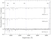 |
Fig. 7. Normalized X-shooter spectra of AzV 261 in the MK classification wavelength range, with key spectral lines marked. Also shown are the archival spectra from Massey et al. (1995) taken in 1992, and from Evans et al. (2004) taken in 1999. A constant is applied for visualisation purposes. |
In addition, in Massey et al. (1995) the authors obtained slit spectra in 13 December 1992 using the Cerro Tololo Interamerican Observatory 4m telescope in the blue-air Schmidt camera. The final data cover the 3900–4800 Å range, at a resolution of 3 Å pixel−1. Based on these spectra the stellar classification is noted by the authors of that paper as O8.5Ie, however a re-classification of the stellar spectrum (show in in Fig. 7) points towards an early B2 supergiant classification (Massey, priv. comm.), agreeing with the classification by Evans et al. (2004). Overall, photometric variability suggests S Doradus candidacy for AzV 261; however, the spectral features themselves do not really agree with this notion. So, we must take and analyse further spectra to find out whether the effective temperature changes between epochs.
3.1. Spectral analysis of AzV 261
3.1.1. Medium-resolution spectroscopy
We obtained medium-resolution spectroscopy with the X-shooter slit spectrograph mounted on the UT2 telescope of the Very Large Telescope (VLT) in Paranal, Chile (see Vernet et al. 2011 for details) on 2017 December 12. The X-shooter spectrograph simultaneously observes the 300–2500 nm wavelength range in medium-resolution (R ∼ 7000) slit spectra using three arms for ultraviolet (UVB; 300–560 nm), visual (VIS; 560–1020 nm) and infrared (1020–2500 nm) wavelength ranges. For the purpose of this study, slit nodding was not used; the infrared observations are thus not usable, due to sky contamination, and were discarded. The spectra were observed in moderate seeing conditions (∼1″) using a slit of of 0.8″ and 0.9″ in the UVB and VIS arm, respectively. The achieved R is 6200 and 7500 in the UVB and VIS arm, respectively. Spectra were reduced using the X-shooter pipeline, with sky subtraction performed using the optimal extraction routine. The final sky-subtracted spectra are given in Fig. 7.
3.1.2. Radial and rotational velocities
Initial stellar radial velocity estimates were obtained from the Doppler shifts of the He I spectrum; the strong Balmer lines were not considered as they had significant emission in their cores. The observed He I lines were fitted using a simple Gaussian plus a low-order polynomial to represent the continuum. As discussed below, there is evidence of some stellar rotational broadening, whilst the diffuse lines (due to 1P−1D and 3P−3D transitions) exhibited significant intrinsic broadening. However, visual inspection showed that the fits appeared to identify the line centre. For transitions between triplet levels, the fine structure multiplet transitions covered a wavelength range corresponding to ∼12–15 km s−1 and in these cases the midpoint wavelength was adopted. Several lines were not considered as they were either very weak (e.g. 4169 Å) or had emission in their wings (e.g. 5876 and 6678 Å). The radial velocity estimates are summarized in Table 2 and have a mean value of 167 ± 11 km s−1.
Radial velocities (vr) and projected rotational velocity (ve sin i) estimates in km s−1 from the He I and metal line spectra.
It was also possible to identify features due to the ions, C II, Mg II, O II, and Si III. However these lines were weak and often blended; additionally, several appeared to be affected by emission near to the line cores (see Figs. 9–11). Radial velocity estimates were found from four metal lines using the same methodology as for the He I spectrum; they are summarized in Table 2. They lead to a radial velocity estimate of 168 ± 5 km s−1, in excellent agreement with that found from the He I spectrum.
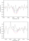 |
Fig. 8. Observed and theoretical profiles for the N II lines at 3995 and 4630 Å. The theoretical profiles have been convolved with a rotational broadening function and are for atmospheric parameters of Teff = 18 000 K and log g = 2.65. The adopted nitrogen abundances are 6.7 (green), 6.9 (blue), and 7.1 (red) dex. Also shown is a theoretical plot for Teff = 16 000 K and log g= 2.45 and a nitrogen abundance of 7.1 dex (dotted red). |
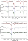 |
Fig. 9. Observed and theoretical profiles for selected wavelength regions. The theoretical profiles have been convolved with a rotational broadening function and are for atmospheric parameters of Teff = 18 000 K and log g = 2.65 (red); Teff = 16 000 K and log g = 2.45 (blue); and Teff = 20 000 K and log g = 2.80 (green). Selected absorption lines are marked, whilst the narrow features at 3933 and 3968 Å are due to interstellar Ca II. |
The intrinsically narrow metal line spectra showed a significant amount of broadening, which could be due to either rotation or to macro-turbulence. Also, the cores of the He I lines were not sharp, again implying additional broadening mechanisms. We have attempted to estimate the contribution of rotational broadening using a Fourier transform (FT) methodology (Simón-Díaz & Herrero 2007), which has been widely used for early-type stars (Dufton et al. 2006, 2013; Lefever et al. 2007; Markova & Puls 2008; Simón-Díaz et al. 2010, 2017; Fraser et al. 2010; Simón-Díaz & Herrero 2014). It relies on the convolution theorem (Gray 2005), namely that the Fourier transform of convolved functions is proportional to the product of their individual Fourier transforms. Then the first minimum in the Fourier transform for an observed spectral line, is assumed to be the first zero in the Fourier transform of the rotational broadening profile. Further details on the implementation of this methodology can be found in for example Simón-Díaz & Herrero (2007) and Dufton et al. (2013), whilst the projected rotational estimates, ve sin i, are listed in Table 2.
Projected rotational velocities were also estimated from the He I spectrum by fitting the profiles of the observed lines, using a Gaussian function (representing the instrumental profile) with a rotational broadening function. Particularly for the diffuse helium lines, the intrinsic broadening may be significant, whilst macro-turbulence and micro-turbulence (Simón-Díaz & Herrero 2014; Simón-Díaz et al. 2010, 2017) may also be significant. These estimates (also listed in Table 2) should thus be considered as upper limits. This is confirmed by the PF estimates for the He I lines being on average 16% larger than their FT equivalents, but they provide a useful check on the FT estimates.
Convincing minima in the FT of the metal lines were only found in two cases with the ve sin i estimates being consistent with those from the He I spectrum. Additionally, no convincing minima could be found for the He I lines at 4437 and 5047 Å, whilst the line at 4921 Å was affected by emission in its red wing. Combining all the available FT estimates yields a mean value of ve sin i = 93 ± 13 km s−1.
3.1.3. Atmospheric modelling
We have employed model-atmosphere grids calculated with the TLUSTY and SYNSPEC codes (Hubeny 1988; Hubeny & Lanz 1995; Hubeny et al. 1998; Lanz & Hubeny 2007). They cover a range of effective temperatures, 10 000 K ≤ Teff ≤ 35 000 K in steps of either 1500 K or 2000 K. Logarithmic gravities (in cm s−2) range from 4.5 dex down to the Eddington limit in steps of 0.25 dex, and micro-turbulences are from 0 to 30 km s−1 in steps of 5 km s−1. As discussed in Ryans et al. (2003) and Dufton et al. (2005), equivalent widths and line profiles interpolated within these grids are in good agreement with those calculated explicitly at the relevant atmospheric parameters.
These non-LTE codes adopt the “classical” stationary model atmosphere assumptions, i.e. plane-parallel geometry, hydrostatic equilibrium, and optical spectrum that is unaffected by winds. The grids assumed a normal helium-to-hydrogen ratio (0.1 by number of atoms) and have been calculated for a range of metallicities; the ratio for an SMC metallicity is used here. However, tests using the Galactic (7.5 dex) or SMC (6.9 dex) grids lead to only small changes in the atmospheric parameters (primarily to compensate for the different amounts of line blanketing). For further information on the TLUSTY grids see Ryans et al. (2003) and Dufton et al. (2005). Obviously, a hydrostatic code like TLUSTY cannot be used to derive wind parameters, and can also not be employed to obtain meaningful fits to wind affected hydrogen lines such as Hα. For these modelling types an alternative code such as CMFGEN or FASTWIND (e.g. Massey et al. 2013) would be needed. However, in the first instance, we are mostly interested in deriving reliable effective temperatures, and comparisons between TLUSTY and FASTWIND have generally shown good agreement between the two codes for effetive temperature estimation (e.g. Trundle et al. 2007).
Initial estimates for the effective temperature and surface gravity could be obtained from fitting the neutral helium and hydrogen spectrum. There is a loci of possible solutions (see e.g. Dufton et al. 1999 for further details), which range from an effective temperature and surface gravity (in cm s−2) of Teff ≃ 16 000 K and log g ≃ 2.40 dex to Teff ≃ 23 000 K and log g ≃ 3.05. For lower effective temperatures the theoretical He I becomes too weak, whilst for higher values the He II spectra would be observable.
This range can be constrained using the observed metal lines and assuming that AzV261 has SMC metal abundances similar to those found in H II regions (see e.g. Kurt & Dufour 1998; Garnett 1999; Carlos Reyes et al. 2015; Toribio San Cipriano et al. 2017) and for other hot stars (see e.g. Venn 1999; Rolleston et al. 2003; Hunter et al. 2007; Trundle et al. 2007), as summarized in Dufton et al. (2005). In Figs. 9–11, observed and theoretical spectra are presented for the wavelength region 3900–4700 Å. The wavelength region 4200–4300 Å is omitted as the only feature observable was the C II 4267 Å doublet, which is subject to complex non-LTE effects (see Sigut 1996; Nieva & Przybilla 2006). The theoretical spectra have been convolved with a Gaussian function to allow for instrumental broadening and with a rotational broadening function with ve sin i = 95 km s−1. A micro-turbulence of 10 km s−1 has been adopted, which is similar to that found in analyses of Magellanic Cloud targets (Hunter et al. 2007; Trundle et al. 2007; McEvoy et al. 2015) with similar effective temperatures and gravities to the locus of estimates found for AzV 261. Spectra for three sets of atmospheric parameters (Teff, log g) are shown: (16 000, 2.45), (18 000, 2.65), and (18 000, 2.80).
Overall the best agreement between observation and theory appears to be for the model with an effective temperature of 18 000 K. Below we discuss the spectra of the different ionic species in more detail.
H I, He I. As discussed above all three models provide a satisfactory fit to the helium spectrum and to the wings of the Balmer lines. The theoretical spectra for the He I line at 3926 Å are too weak, possibly due to the adoption of a semi-classical quasi-static approximation for the line broadening (Dimitrijevic & Sahal-Brechot 1984). Additionally, the theoretical profiles for the He I line at 4713 Å appear to be too strong, although the observed profiles may exhibit emission in its wings. The lack of significant He II absorption in all the theoretical spectra (e.g. at 4541 and 4686 Å) is also consistent with the observations.
C II. For the gravities considered here, the C II spectrum has a maximum strength at Teff ≃ 20 000 K. As such it shows little variation in the theoretical spectrum, with the doublet at 4267 Å being in good agreement with observation. As discussed above, the doublet at 4267 Å is difficult to model, and indeed all our theoretical spectra are stronger than observed, which is consistent with previous investigations using this model grid (Trundle et al. 2007; Hunter et al. 2007).
N II. The theoretical spectra adopt a nitrogen abundance of 7.1 dex, which is higher than that found in H II regions (e.g. 6.55 dex; Carlos Reyes et al. 2015) or the lowest stellar abundances (e.g. 6.66 dex; Rolleston et al. 2003). It was chosen to be representative of the typical nitrogen enrichment observed in SMC B-type stars (Trundle et al. 2007; Hunter et al. 2007) and as such it provides no constraint on the atmospheric parameters. However, the reasonable agreement between theory and observation for the N II line at 3995 Å argues against any large nitrogen enhancement.
O II. There is a rich O II spectrum with some of the stronger features identified in Figs. 1–3; additionally, most of the unidentified absorption features are also due to this ion. The theoretical line strengths are sensitive to the adopted effective temperature and the model with Teff = 18 000 K provides the best overall agreement with observation.
Mg II. The doublet at 4481 Å is too strong in all three theoretical spectrum. However, the observed profile appears to be affected by emission in both wings making any comparison problematic. Si II, Si III. The Si II doublet at 4128–4130 Å appears to be very weak in the observed spectrum. The spectra for the two hotter models appear consistent with the observations. The Si III triplet transitions between 4552 and 4574 Å are best fitted by the theoretical spectrum with Teff = 18 000 K, although the other spectra also provide acceptable fits.
In summary the model with Teff = 18 000 K provides the best overall fit to the spectrum, and we estimate a stochastic error of ±2000 K. This error would translate into an error of ∼0.2 dex in the gravity. Combining this in quadrature with a fitting uncertainty of ∼0.2 dex leads to an error in the gravity of ±0.3 dex. Hence our best estimate of the atmospheric parameters and their errors are Teff = 18 000 ± 2000 K and log g = 2.65 ± 0.3 dex.
As discussed above, the strength of the N II spectrum is close to or below the limit for detection. As nitrogen is important for constraining the evolutionary status of early-type stars, we have attempted to set an upper limit on its abundance. Several N II lines can be seen in B-type spectra, especially for targets showing significant nitrogen enrichments (see e.g. Dufton et al. 2018). In Fig. 8 we show the two intrinsically strongest features at 3995 Å and 4630 Å that are not significantly affected by blending (Dufton et al. 2018), together with theoretical profiles, which are for our adopted atmospheric parameters and have been convolved with a rotational broadening functions and are for nitrogen abundances between 6.7 and 7.1 dex. The observational and theoretical profiles were normalized in an identical fashion by a least-squares fitting of a linear polynomial to continuum regions at ±3–5 Å from the line centre.
There is marginal evidence for an observed N II line at 3995 Å and this would imply a nitrogen abundance of ∼6.7 dex. Alternatively, a conservative upper limit for the nitrogen abundance would appear to be 7.1 dex. The N II at 4630 Å is not seen again, implying a similar upper limit on the nitrogen abundance. Adopting a baseline nitrogen abundance of 6.6 dex (Carlos Reyes et al. 2015; Rolleston et al. 2003; Trundle et al. 2007; Hunter et al. 2007) would then imply a nitrogen enhancement of ≤0.5 dex Uncertainties due to possible errors in the atmospheric parameters are dominated by the uncertainty due to the effective temperature. This is illustrated in Fig. 8 where a theoretical profile is shown for an effective temperature of 16 000 K (and log g = 2.45 dex). Adopting this lower effective temperature would increase the abundance limits by approximately 0.4 dex.
The estimation of the atmospheric parameters depends particularly on the assumption of baseline abundances for helium, oxygen, and silicon. It is unlikely that the silicon abundance has been effected by nucleosynthetic process since the star formed. However, the other two elements could be affected by the mixing of material processed by the CNO bi-cycle to the surface. Adopting a nitrogen enhancement of 0.5 dex, the SMC models of Brott et al. (2011) imply changes in the helium and oxygen abundances of less than <0.01 and <0.04 dex for masses between 15M⊙ and 60M⊙. Increasing the nitrogen enhancement to 0.9 dex (i.e. allowing for possible errors in the effective temperature) would lead to changes of <0.02 and <0.09 dex. This implies that our use of a normal SMC abundance should not be a major source of error.
3.1.4. Hα line profile
The Hα line strength and profile in Bsgs is a key indicator of mass loss via stellar winds. The rate of mass loss is still under debate, with differences in measured mass-loss rates varying by up to factors of 10 from different indicators (e.g. the Hα line vs. ultraviolet P Cygni lines), which occurs because clumping in the winds significantly affects the profile shapes of emission lines, including Hα. In addition, stellar pulsations in Bsgs may be linked to periods of enhanced mass loss.
The Hα emission line strength (Fig. 12) changes from −22.4 ± 1.2 Å in the 1999 Evans et al. spectra to −38.5 ± 0.3 Å in 2017 X-shooter spectra. It is clear that AzV 261 displays a variable stellar wind, although the model fits to observations may not result in accurate mass-loss rates due to the choice of models (e.g. TLUSTY). If the sky subtraction for the multi-fibre spectroscopy of Evans et al. (2004) is poor, the measured equivalent width would be higher from their spectrum. Their equivalent width estimate is in fact lower, implying that uncertainties in the sky subtraction cannot explain the difference. We do not fit more sophisticated model atmospheres as we are merely interested in observing a change in spectral type (rather than wind variability) in order to determine whether AzV 261 is a S Doradus variable. Regarding the absence of P Cyg absorption, this actually suggests that the star is hotter than the bi-stability jump of 21 000 K, as absorption appears at and below the jump (Petrov et al. 2014).
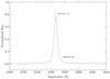 |
Fig. 12. Normalized Hα line profile from the X shooter spectra taken in 2017 December (red) and archival spectra from Evans et al. (2004) taken in 1999 September shown as solid blue lines. The emission line equivalent width increased by −16.1 Å within this period. We note that if the sky subtraction from the Evans et al. (2004) fibre spectra is poor, this difference will only be magnified. |
3.2. Circumstellar dust
Most S Doradus LBV variables show evidence of excess free-free emission (Humphreys et al. 2017a,b; de Wit et al. 2014). In contrast with evolved supergiant B[e] (sgB[e]), and warm hypergiant stars, they do not display evidence of warm dust. Compared to the other Hα emitting objects in the Bsgs zoo, S Doradus variables therefore have excess free-free emission resembling that of classical Be (cBe) stars (which are main sequence fast rotators).
We can therefore use the infrared colour–colour diagrams to distinguish AzV 261 from other objects in the Bsgs zoo. In Fig. 13a, we plot the near-infrared (J−H) vs. (H−K s) colour–colour diagram showing the position of known S Doradus variables, sgB[e], warm hypergiants, cBe stars (taken from Humphreys et al. 2017a), and Bsgs in our sample. Also shown is the main sequence locus at SMC metallicity taken from Kalari et al. (2018). In addition, we also show the data in the mid-infrared (from Humphreys et al. 2017a) for the same stars in the [3.6 μm]–[4.5 μm] vs. [5.8 μm]–[8.0 μm] mid-infrared colour–colour diagram. From these diagrams, AzV 261 exhibits modest free-free emission at levels similar to other known S Doradus LBVs at the higher end of those exhibited by cBe stars. In Fig. 14, we plot the spectral energy distribution of AzV 261 along with the TLUSTY model atmosphere for the best-fit stellar parameters. The best-fit model for the infrared excess is a black body of Tb = 2550 K. The position of AzV 261 in infrared colour–colour diagrams, and its spectral energy distribution point towards free-free emission.
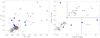 |
Fig. 13. Left: near-infrared (J−H) vs. (H−K s) colour–colour diagram of known sgB[e] (open squares), warm hypergiants (open triangles), cBe stars (open circles), known S Doradus variables (blue dots), BSgs (small dots), and AzV 261 (red asterisk). Data taken from Humphreys et al. (2017a). The dashed red line is the main sequence locus at SMC metallicity. Right: mid-infrared [3.6 μm]–[4.5 μm] vs. [5.8 μm]–[8.0 μm] colour–colour diagram. Symbols are as in the left panel. The position of AzV 261 in both diagrams suggests the presence of free–free emission. The LBVs redward of colours [5.8 μm]–[8.0 μm] > 1.0 are contaminated by polycyclic aromatic hydrocarbon emission from nebulosity, with the regions of nebular contamination and dusty stars indicated following Humphreys et al. (2017a). |
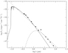 |
Fig. 14. Spectral energy distribution of AzV 261 covering photometry from the literature from U-8.0 μm. Overplotted as a solid line is the TLUSTY model atmosphere for the best-fit stellar parmeters of Teff = 18 000 K, log g = 2.5. The infrared-excess, corresponding to possible free-free emission of cold dust is best fit using a black-body model having Tb = 2550 K (shown as the dashed line). The dotted line is of constant frequency flux density normalized to the 3.6 μm photometry to make the free-free contribution clearer. |
Since the spectroscopic analysis of the surface gravity precludes the possibility that AzV 261 is a cBe star, it is most likely a S Doradus variable based on its photometric variability and infrared colours. However, the absence of spectroscopic variability is puzzling. Based on the absence of spectral non-variability AzV 261 is not a LBV S Doradus variable.
3.3. AzV 261 within the Bsgs zoo
Based on the observed properties of AzV 261, we attempt to classify AzV 261 within the Bsgs zoo (assuming that it may be a S Doradus LBV). Bsgs are diverse, but we attempt to classify AzV 261 between the main types, namely (i) Bsgs, (ii) sgB[e], and (iii) S Doradus LBV variables. In addition, we include the (iv) cBe classification, although we note that cBe stars are main sequence stars. The main classifying properties of AzV 261 are (i) a supergiant luminosity classification, (ii) no effective temperature variations, (iii) aperiodic increase/decrease in brightness interspersed with periodic micro-variations, (iv) single-peaked Hα line emission, and (v) infrared excess resembling free-free emission due to cold circumstellar disc/ejecta.
In Table 3, we list the properties of the different Bsg subtypes, together with those for AzV 261. In general they agree best with an S Doradus classification apart from the lack of characteristic temperature variability seen in most S Doradus LBV variables, which remains puzzling. Finally, we note that AzV 261 displays an extremely low luminosity for a S Doradus LBV variable (of logarithm of luminosity log L = 4.9 ± 0.1 L⊙), which implies a stellar mass of  according to the models of Brott et al. (2011). This places AzV 261 at the low-mass end of known S Doradus LBV variables.
Properties of AzV 261 among the Bsg zoo and cBe stars.
In Fig. 15, we plot the position of AzV 261 and the Bsgs studied here in the Hertzsprung–Russell diagram with respect to stellar tracks from Brott et al. (2011), along with known S Doradus variables in the SMC, LMC, and the Milky Way. The effective temperatures and bolometric corrections (to calculate the luminosities of the Bsgs) were estimated using the spectral type-effective temperature scale of Trundle et al. (2007), and computed following the procedure described in McEvoy et al. (2015). The data for the luminosities and effective temperatures of the literature S Doradus variables here were taken from Smith et al. (2018), who present revised distances and luminosities for known galactic S Doradus variables using recent Gaia DR2 parallaxes. Their results identify a population of low-luminosity confirmed S Doradus variables in the galaxy which do not have extragalactic counterparts (e.g. W 243 and HD 168607). The authors of that paper suggest that a systematic search for new S Doradus variables in external galaxies might well uncover new low-luminosity LBVs, such as those shown here. The existence of these low-luminosity S Doradus LBV variables in the Milky Way and in the SMC suggest the existence of a different instability mechanism, with important implications for SNe (see Smith et al. 2018). However, we consider it unlikely that AzV 261 is a member of this group since it does not show the characteristic temperature variations seen in other LBVs.
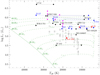 |
Fig. 15. Position of AzV 261 on the Hertzsprung–Russell diagram marked by the red asterisk, along the Bsgs studied here as grey squares. The positions of confirmed LBVs from the literature in the galaxy (black circles), LMC (blue circles), and the SMC (red circle) are also shown. Cyan circles mark the position of known LBVs in M31 and M33 (from Humphreys et al. 2017b). The dashed green lines are the stellar tracks from Brott et al. (2011) with the corresponding initial stellar mass indicated, and the solid line is the zero-age main sequence isochrone. |
4. Discussion: S Doradus variables among the Bsg population
The key question we wish to address is whether Bsgs are fundamentally dormant LBVs or if they represent separate stellar populations, which would make bona fide S Doradus LBVs “special objects”.
Although individual LBVs and LBV candidates have been discovered at metallicities that are potentially even lower than that of the SMC (Drissen et al. 2001; Izotov & Thuan 2008; Pustilnik et al. 2008; Herrero et al. 2010; Bomans & Weis 2011), in this systematic study of the SMC we found just one S Doradus candidate out of a total of 64 Bsgs.
If we assume that all Bsgs pass through the S Doradus phase in their lifetimes, we can set an upper limit to the duration of the S Doradus phase. Assuming that the mean duration between the end of the H-burning lifetime of a massive star and the onset of the Wolf–Rayet phase is ∼105 yr, and that all Bsgs become S Doradus variables, we expect the duration of the S Doradus phase at SMC metallicities to be ∼103 yr. This is much lower than the number suggested if Bsgs were truly dormant S Doradus variables (Massey 2006; Smith 2015) where their predicted evolutionary lifetime is ∼105 yr, but also lower than that determined in the standard picture of massive star evolution ∼104 yr (Humphreys & Davidson 1994; Conti 1976).
The low incidence of LBVs in the SMC seems to suggest that Bsgs and S Doradus LBVs are truly different from one another, and that not all Bsgs become S Doradus variables. This may suggest that the search for Hα P Cygni profiles, as suggested by Massey et al. (2007), might not provide the answer to the total duration of the LBV phase in massive star evolution. However it might still be possible that related searches at high spectral resolution, allowing the presence of multiple-troughed P Cygni absorption components to be revealed, may become an efficient tool for detecting extra-galactic LBVs, as suggested by Groh & Vink (2011).
Additional evidence for an intrinsic difference between Bsgs and S Doradus variables comes from the complete absence of rapidly rotating Bsgs with ve sin i ≳ 200 km s−1 (see Vink et al. 2010), whilst several S Doradus variables have been found to be rotating rather rapidly (Groh et al. 2006, 2009). For this reason Justham et al. (2014) considered stellar merging to be a likely evolutionary path to produce LBV supernovae.
The small number of confirmed LBVs in the SMC represents a puzzle; enhanced LBV mass loss seems to be required if canonical stationary wind mass loss from normal stars is reduced at the lower metal content of the SMC (Mokiem et al. 2007). This raises the question of whether the known population of evolved Wolf–Rayet stars in the SMC have been produced by rotationally induced chemical homogeneous evolution (Brott et al. 2011; but see Vink & Harries 2017) or by binary interactions (Schootemeijer & Langer 2018; but see Shenar et al. 2016).
Finally, Vink (2018) recently performed radiative transfer computations with a dynamic version of the Monte Carlo method to study the bi-stability jump of LBVs as a function of metallicity. He found the bi-stability jump to be smaller at low metallicity. These results may be related to the low number of S Doradus variables in the SMC that we find here. Metal-poor galaxies are generally lower mass and less luminous than their metal-rich counterparts, resulting in a smaller absolute population of massive stars (although recent evidence for a top-heavy stellar initial mass function at low metallicities compared to a Salpeter mass function suggests that the relative fraction of massive stars may be higher; e.g. Kalari et al. 2018; Schneider et al. 2018). Therefore, short-lived phases such as LBVs might become harder to observe serendipitously, thus the systematic approach like the one presented here carries important weight in defining whether the incidence and characteristics of LBV S Doradus variables do indeed vary by metallicity, how this influences our view of stellar evolution in the early Universe, and how LBVs evolve.
5. Conclusions
In this paper, we presented a systematic search for S Doradus variables among the Bsgs population in the 1/5 Z⊙ SMC. We conducted our search using light curves spread across three years (with a cadence of one night) of 64 Bsgs from a total known Bsgs population of 110 in the SMC within our field of view.
Our motivation was to identify whether all Bsgs display dormant LBV behaviour at differing timescales or amplitudes, or whether S Doradus LBV variables are truly unique objects. From examining the light curves of the 64 SMC Bsgs, only one Bsg, AzV 261 demonstrated S Doradus-like photometric variability. AzV 261 did not display variation in the spectral type. Therefore, AzV 261 is not a LBV S Doradus variable. Our findings imply that the duration of the LBV phase is ∼103 yr, or more likely that S Doradus LBVs and Bsgs are likely intrinsically different objects.
Data are from the American Association of Variable Star Observers International Database, at http://www.aavso.org
Acknowledgments
The authors thank the referee, R. Humphreys, for insightful comments. We are grateful to C.J. Evans, and P. Massey for kindly providing their spectra of AzV 261. The authors also thank L. Wyrzykowski and the OGLE consortium for providing their data. V.M.K. also thanks G. Blanc, K. Boutsia, and N. Morrell for collecting a spectrum from Las Campanas. The authors thank ESO for providing Directors Discretionary time to perform the X-shooter observations. V.M.K. acknowledges support from the FONDECYT-CONICYT grant No. 3160117. M.F. is supported by a Royal Society – Science Foundation Ireland University Research Fellowship. We acknowledge with thanks the variable star observations from the AAVSO International Database contributed by observers worldwide and used in this research.
References
- Abbott, B. P., Abbott, R., Abbott, T. D., et al. 2016, ApJ, 833, L1 [NASA ADS] [CrossRef] [Google Scholar]
- Bomans, D. J., & Weis, K. 2011, Bull. Soc. R. Sci. Liège, 80, 341 [NASA ADS] [Google Scholar]
- Bonanos, A. Z., Lennon, D. J., Köhlinger, F., et al. 2010, AJ, 140, 416 [NASA ADS] [CrossRef] [Google Scholar]
- Brott, I., de Mink, S. E., Cantiello, M., et al. 2011, A&A, 530, A115 [NASA ADS] [CrossRef] [EDP Sciences] [Google Scholar]
- Carlos Reyes, R. E., Reyes Navarro, F. A., Meléndez, J., Steiner, J., & Elizalde, F. 2015, Rev. Mex. Astron. Astrofis., 51, 135 [NASA ADS] [Google Scholar]
- Chiosi, C., & Maeder, A. 1986, ARA&A, 24, 329 [NASA ADS] [CrossRef] [Google Scholar]
- Conti, P. S. 1976, Mem. Soc. R. Sci. Liège, 9, 193 [NASA ADS] [Google Scholar]
- de Vaucouleurs, G., & Eggen, O. J. 1952, PASP, 64, 185 [NASA ADS] [CrossRef] [Google Scholar]
- de Wit, W. J., Oudmaijer, R. D., & Vink, J. S. 2014, Adv. Astron., 2014, 270848 [NASA ADS] [CrossRef] [Google Scholar]
- Dimitrijevic, M. S., & Sahal-Brechot, S. 1984, J. Quant. Spectr. Rad. Transf., 31, 301 [NASA ADS] [CrossRef] [Google Scholar]
- Drissen, L., Crowther, P. A., Smith, L. J., et al. 2001, ApJ, 546, 484 [NASA ADS] [CrossRef] [Google Scholar]
- Dufton, P. L., Smartt, S. J., & Hambly, N. C. 1999, A&AS, 139, 231 [NASA ADS] [CrossRef] [EDP Sciences] [Google Scholar]
- Dufton, P. L., Ryans, R. S. I., Trundle, C., et al. 2005, A&A, 434, 1125 [NASA ADS] [CrossRef] [EDP Sciences] [Google Scholar]
- Dufton, P. L., Ryans, R. S. I., Simón-Díaz, S., Trundle, C., & Lennon, D. J. 2006, A&A, 451, 603 [NASA ADS] [CrossRef] [EDP Sciences] [Google Scholar]
- Dufton, P. L., Langer, N., Dunstall, P. R., et al. 2013, A&A, 550, A109 [NASA ADS] [CrossRef] [EDP Sciences] [Google Scholar]
- Dufton, P. L., Thompson, A., & Crowther, P. A. 2018, A&A, 615, A101 [NASA ADS] [CrossRef] [EDP Sciences] [Google Scholar]
- Evans, C. J., Howarth, I. D., Irwin, M. J., Burnley, A. W., & Harries, T. J. 2004, MNRAS, 353, 601 [NASA ADS] [CrossRef] [Google Scholar]
- Findeisen, K., Cody, A. M., & Hillenbrand, L. 2015, ApJ, 798, 89 [NASA ADS] [CrossRef] [Google Scholar]
- Fraser, M., Dufton, P. L., Hunter, I., & Ryans, R. S. I. 2010, MNRAS, 404, 1306 [NASA ADS] [Google Scholar]
- Frescura, F. A. M., Engelbrecht, C. A., & Frank, B. S. 2007, ApJ, submitted, DOI: 10.1016/j.icarus.2012.06.015 [Google Scholar]
- Gal-Yam, A., & Leonard, D. C. 2009, Nature, 458, 865 [NASA ADS] [CrossRef] [PubMed] [Google Scholar]
- Garnett, D. R. 1999, New Views Magellanic Clouds, 190, 266 [Google Scholar]
- Gräfener, G., Owocki, S. P., & Vink, J. S. 2012, A&A, 538, A40 [NASA ADS] [CrossRef] [EDP Sciences] [Google Scholar]
- Gray, D. F. 2005, in The Observation and Analysis of Stellar Photospheres, 3rd edn. (Cambridge, UK: Cambridge University Press) [Google Scholar]
- Groh, J. H., & Vink, J. S. 2011, A&A, 531, L10 [NASA ADS] [CrossRef] [EDP Sciences] [Google Scholar]
- Groh, J. H., Hillier, D. J., & Damineli, A. 2006, ApJ, 638, L33 [NASA ADS] [CrossRef] [Google Scholar]
- Groh, J. H., Damineli, A., Hillier, D. J., et al. 2009, ApJ, 705, L25 [NASA ADS] [CrossRef] [Google Scholar]
- Groh, J. H., Meynet, G., & Ekström, S. 2013, A&A, 550, L7 [NASA ADS] [CrossRef] [EDP Sciences] [Google Scholar]
- Gvaramadze, V. V., Kniazev, A. Y., Miroshnichenko, A. S., et al. 2012, MNRAS, 421, 3325 [NASA ADS] [CrossRef] [Google Scholar]
- Herrero, A., Garcia, M., Uytterhoeven, K., et al. 2010, A&A, 513, A70 [NASA ADS] [CrossRef] [EDP Sciences] [Google Scholar]
- Hubeny, I. 1988, Comput. Phys. Commun., 52, 103 [NASA ADS] [CrossRef] [Google Scholar]
- Hubeny, I., & Lanz, T. 1995, ApJ, 439, 875 [Google Scholar]
- Hubeny, I., Heap, S. R., & Lanz, T. 1998, Prop. Hot Luminous Stars, 131, 108 [Google Scholar]
- Humphreys, R. M., & Davidson, K. 1994, PASP, 106, 1025 [NASA ADS] [CrossRef] [Google Scholar]
- Humphreys, R. M., Weis, K., Davidson, K., & Gordon, M. S. 2016, ApJ, 825, 64 [NASA ADS] [CrossRef] [Google Scholar]
- Humphreys, R. M., Gordon, M. S., Martin, J. C., Weis, K., & Hahn, D. 2017a, ApJ, 836, 64 [NASA ADS] [CrossRef] [Google Scholar]
- Humphreys, R. M., Davidson, K., Hahn, D., Martin, J. C., & Weis, K. 2017b, ApJ, 844, 40 [NASA ADS] [CrossRef] [Google Scholar]
- Hunter, I., Dufton, P. L., Smartt, S. J., et al. 2007, A&A, 466, 277 [NASA ADS] [CrossRef] [EDP Sciences] [Google Scholar]
- Izotov, Y. I., & Thuan, T. X. 2008, ApJ, 687, 133 [NASA ADS] [CrossRef] [Google Scholar]
- Justham, S., Podsiadlowski, P., & Vink, J. S. 2014, ApJ, 796, 121 [NASA ADS] [CrossRef] [Google Scholar]
- Kalari, V. M., Carraro, G., Evans, C. J., & Rubio, M. 2018, ApJ, 857, 132 [NASA ADS] [CrossRef] [Google Scholar]
- Kotak, R., & Vink, J. S. 2006, A&A, 460, L5 [NASA ADS] [CrossRef] [EDP Sciences] [Google Scholar]
- Kourniotis, M., Bonanos, A. Z., Soszyński, I., et al. 2014, A&A, 562, A125 [NASA ADS] [CrossRef] [EDP Sciences] [Google Scholar]
- Kurt, C. M., & Dufour, R. J. 1998, Rev. Mex. Astron. Astrofis. Conf. Ser., 7, 202 [Google Scholar]
- Labadie-Bartz, J., Pepper, J., McSwain, M. V., et al. 2017, AJ, 153, 252 [NASA ADS] [CrossRef] [Google Scholar]
- Lamers, H. J. G. L. M., Bastiaanse, M. V., Aerts, C., & Spoon, H. W. W. 1998, A&A, 335, 605 [NASA ADS] [Google Scholar]
- Langer, N. 2012, ARA&A, 50, 107 [NASA ADS] [CrossRef] [Google Scholar]
- Lanz, T., & Hubeny, I. 2007, ApJS, 169, 83 [CrossRef] [Google Scholar]
- Lefever, K., Puls, J., & Aerts, C. 2007, A&A, 463, 1093 [NASA ADS] [CrossRef] [EDP Sciences] [Google Scholar]
- Lenz, P., & Breger, M. 2005, Commun. Asteroseismol., 146, 53 [NASA ADS] [CrossRef] [Google Scholar]
- Mahabal, A. A., Djorgovski, S. G., Drake, A. J., et al. 2011, Bull. Astron. Soc. India, 39, 387 [NASA ADS] [Google Scholar]
- Markova, N., & Puls, J. 2008, A&A, 478, 823 [NASA ADS] [CrossRef] [EDP Sciences] [Google Scholar]
- Massey, P. 2006, ApJ, 638, L93 [NASA ADS] [CrossRef] [Google Scholar]
- Massey, P., Lang, C. C., Degioia-Eastwood, K., & Garmany, C. D. 1995, ApJ, 438, 188 [NASA ADS] [CrossRef] [Google Scholar]
- Massey, P., McNeill, R. T., Olsen, K. A. G., et al. 2007, AJ, 134, 2474 [NASA ADS] [CrossRef] [Google Scholar]
- Massey, P., Neugent, K. F., Hillier, D. J., & Puls, J. 2013, ApJ, 768, 6 [NASA ADS] [CrossRef] [Google Scholar]
- McEvoy, C. M., Dufton, P. L., Evans, C. J., et al. 2015, A&A, 575, A70 [NASA ADS] [CrossRef] [EDP Sciences] [Google Scholar]
- Miroshnichenko, A. S. 2006, Stars B[e] Phenom., 355, 13 [NASA ADS] [Google Scholar]
- Mokiem, M. R., de Koter, A., Vink, J. S., et al. 2007, A&A, 473, 603 [NASA ADS] [CrossRef] [EDP Sciences] [Google Scholar]
- Nieva, M. F., & Przybilla, N. 2006, ApJ, 639, L39 [NASA ADS] [CrossRef] [Google Scholar]
- Petrov, B., Vink, J. S., & Gräfener, G. 2014, A&A, 565, A62 [NASA ADS] [CrossRef] [EDP Sciences] [Google Scholar]
- Puls, J., Vink, J. S., & Najarro, F. 2008, A&ARv, 16, 209 [NASA ADS] [CrossRef] [EDP Sciences] [Google Scholar]
- Pustilnik, S. A., Tepliakova, A. L., Kniazev, A. Y., & Burenkov, A. N. 2008, MNRAS, 388, L24 [NASA ADS] [CrossRef] [Google Scholar]
- Rolleston, W. R. J., Venn, K., Tolstoy, E., & Dufton, P. L. 2003, A&A, 400, 21 [NASA ADS] [CrossRef] [EDP Sciences] [Google Scholar]
- Ryans, R. S. I., Dufton, P. L., Mooney, C. J., et al. 2003, A&A, 401, 1119 [NASA ADS] [CrossRef] [EDP Sciences] [Google Scholar]
- Schneider, F. R. N., Sana, H., Evans, C. J., et al. 2018, Science, 359, 69 [NASA ADS] [CrossRef] [Google Scholar]
- Schootemeijer, A., & Langer, N. 2018, A&A, 611, A75 [NASA ADS] [CrossRef] [EDP Sciences] [Google Scholar]
- Shenar, T., Hainich, R., Todt, H., et al. 2016, A&A, 591, A22 [NASA ADS] [CrossRef] [EDP Sciences] [Google Scholar]
- Sigut, T. A. A. 1996, ApJ, 473, 452 [NASA ADS] [CrossRef] [Google Scholar]
- Simón-Díaz, S., & Herrero, A. 2007, A&A, 468, 1063 [NASA ADS] [CrossRef] [EDP Sciences] [Google Scholar]
- Simón-Díaz, S., & Herrero, A. 2014, A&A, 562, A135 [NASA ADS] [CrossRef] [EDP Sciences] [Google Scholar]
- Simón-Díaz, S., Herrero, A., Uytterhoeven, K., et al. 2010, ApJ, 720, L174 [NASA ADS] [CrossRef] [Google Scholar]
- Simón-Díaz, S., Godart, M., Castro, N., et al. 2017, A&A, 597, A22 [NASA ADS] [CrossRef] [EDP Sciences] [Google Scholar]
- Smith, N. 2014, ARA&A, 52, 487 [NASA ADS] [CrossRef] [MathSciNet] [Google Scholar]
- Smith, N. 2015, Very Massive Stars Local Univ., 412, 227 [NASA ADS] [Google Scholar]
- Smith, N., & Owocki, S. P. 2006, ApJ, 645, L45 [NASA ADS] [CrossRef] [Google Scholar]
- Smith, N., & Tombleson, R. 2015, MNRAS, 447, 598 [NASA ADS] [CrossRef] [Google Scholar]
- Smith, N., Aghakhanloo, M., & Murphy, J. W. 2018, ArXiv e-prints [arXiv:1805.03298] [Google Scholar]
- Szymanski, M. K. 2005, Acta Astron., 55, 43 [NASA ADS] [Google Scholar]
- Toribio San Cipriano, L., Domínguez-Guzmán, G., Esteban, C., et al. 2017, MNRAS, 467, 3759 [NASA ADS] [CrossRef] [Google Scholar]
- Trundle, C., Dufton, P. L., Hunter, I., et al. 2007, A&A, 471, 625 [NASA ADS] [CrossRef] [EDP Sciences] [Google Scholar]
- Trundle, C., Kotak, R., Vink, J. S., & Meikle, W. P. S. 2008, A&A, 483, L47 [NASA ADS] [CrossRef] [EDP Sciences] [Google Scholar]
- Udalski, A., Kubiak, M., & Szymanski, M. 1997, Acta Astron., 47, 319 [NASA ADS] [Google Scholar]
- VanderPlas, J. T. 2018, ApJS, 236, 16 [NASA ADS] [CrossRef] [Google Scholar]
- van Genderen, A. M. 2001, A&A, 366, 508 [NASA ADS] [CrossRef] [EDP Sciences] [Google Scholar]
- Venn, K. A. 1999, ApJ, 518, 405 [NASA ADS] [CrossRef] [Google Scholar]
- Vernet, J., Dekker, H., D’Odorico, S., et al. 2011, A&A, 536, A105 [NASA ADS] [CrossRef] [EDP Sciences] [Google Scholar]
- Vink, J. S. 2012, Eta Carinae Supernova Impostors, 384, 221 [Google Scholar]
- Vink, J. S. 2015, Very Massive Stars Local Univ., 412 [Google Scholar]
- Vink, J. S. 2018, A&A, submitted [arXiv:1808.06612] [Google Scholar]
- Vink, J. S., & Harries, T. J. 2017, A&A, 603, A120 [NASA ADS] [CrossRef] [EDP Sciences] [Google Scholar]
- Vink, J. S., & de Koter, A. 2005, A&A, 442, 587 [NASA ADS] [CrossRef] [EDP Sciences] [Google Scholar]
- Vink, J. S., de Koter, A., & Lamers, H. J. G. L. M. 2001, A&A, 369, 574 [NASA ADS] [CrossRef] [EDP Sciences] [Google Scholar]
- Vink, J. S., Brott, I., Gräfener, G., et al. 2010, A&A, 512, L7 [NASA ADS] [CrossRef] [EDP Sciences] [Google Scholar]
- Woosley, S. E., & Heger, A. 2015, Very Massive Stars Local Univ., 412, 199 [NASA ADS] [Google Scholar]
Appendix A: Light curves of Bsgs that have data from the OGLE II survey
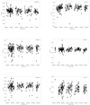 |
Fig. A.1. Light curves of 63 Bsgs that have data from the OGLE II survey. The Julian date is plotted against the measured I-band magnitude. |
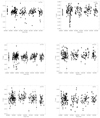 |
Fig. A.1. continued. |
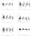 |
Fig. A.1. continued. |
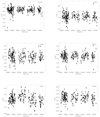 |
Fig. A.1. continued. |
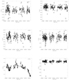 |
Fig. A.1. continued. |
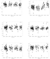 |
Fig. A.1. continued. |
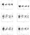 |
Fig. A.1. continued. |
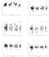 |
Fig. A.1. continued. |
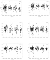 |
Fig. A.1. continued. |
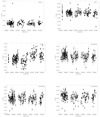 |
Fig. A.1. continued. |
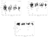 |
Fig. A.1. continued. |
Appendix B: Lomb–Scargle periodogram of Bsgs that have OGLE II data
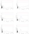 |
Fig. B.1. Lomb–Scargle periodogram of 64 Bsgs. The period in days is plotted against the power. The red and blue lines respectively represent the 99% and 95% significance calculated from the Monte Carlo bootstrap simulations. |
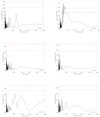 |
Fig. B.1. continued. |
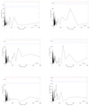 |
Fig. B.1. continued. |
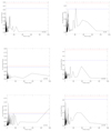 |
Fig. B.1. continued. |
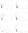 |
Fig. B.1. continued. |
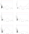 |
Fig. B.1. continued. |
 |
Fig. B.1. continued. |
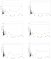 |
Fig. B.1. continued. |
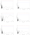 |
Fig. B.1. continued. |
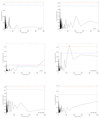 |
Fig. B.1. continued. |
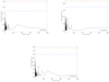 |
Fig. B.1. continued. |
Appendix C: δm–δt two-dimensional histogram of Bsgs with OGLE II data
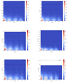 |
Fig. C.1. Two-dimensional histogram of the δm–δt plot of 64 Bsgs. The δm in mag is plotted against the δt in days, and the colour is indicative of the density of the histogram following the colourbar. |
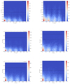 |
Fig. C.1. continued. |
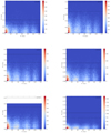 |
Fig. C.1. continued. |
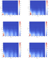 |
Fig. C.1. continued. |
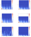 |
Fig. C.1. continued. |
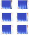 |
Fig. C.1. continued. |
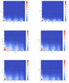 |
Fig. C.1. continued. |
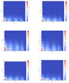 |
Fig. C.1. continued. |
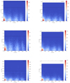 |
Fig. C.1. continued. |
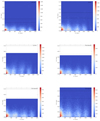 |
Fig. C.1. continued. |
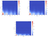 |
Fig. C.1. continued. |
All Tables
Radial velocities (vr) and projected rotational velocity (ve sin i) estimates in km s−1 from the He I and metal line spectra.
All Figures
|
Fig. 1. Recovered spectral types of Bsgs in our sample (red) and the total number of Bsgs in the SMC (solid line) within the OGLE II survey area. |
| In the text | |
|
Fig. 2. Representative light curve of the Bsg 2dFS0153 from the OGLE survey, where the measured OGLE I-band magnitude is plotted against the Julian Date. Light curves of all 64 Bsgs in our sample are shown in Fig. A.1. |
| In the text | |
|
Fig. 3. Representative Lomb–Scargle periodogram of Bsg 2dFS0153. The period in days is plotted against the Lomb–Scargle power. The dashed red and blue lines are the 99% and 95% significance levels identified using the bootstrap Monte Carlo simulations. Periodic variables are those whose peak in the power spectrum is greater than the 99% significance level. Lomb–Scargle periodograms of the remaining 63 Bsgs are displayed in Fig. B.1. |
| In the text | |
|
Fig. 4. Two-dimensional histogram (δm–δt) of the Bsg 2dFS1053 from the OGLE II data, where the colour gradient marks the density of the points (see the colourbar). The dashed line marks the 10σ level of the random photometric uncertainty, while the solid line differentiates variations above the 0.1m level. The δm–δt two-dimensional histograms of the remaining Bsgs are included in Fig. C.1. |
| In the text | |
|
Fig. 5. Two-dimensional histogram (δm–δt) of known S Doradus variables R 40, R 110, S Doradus on (panel a), (panel b) and (panel c) respectively. The candidate S Doradus variable in our Bsgs sample, AzV 261 is shown in (panel d). Symbols are same as Fig. 4. |
| In the text | |
|
Fig. 6. Top: I-band light curve of AzV 261 spanning from 1998 to 2009. Also shown is the scaled historical light curve of the classic LBV star S Doradus for comparison (crosses). Panel b: (V−I) colour plotted against the Julian date for AzV 261. Middle: (panel a) light curve with the overall trend removed by a fourth-degree polynomial, with the best-fit predicted light curve (the three peaks are given in Table 1). Panel b: residuals between the fit period and the observed light curve. Bottom: V vs. (V−I) colour-magnitude diagram of AzV 261 over time, with time given by the colourbar. The behaviour of a brightness increase corresponding to a temperature decrease is seen here. |
| In the text | |
|
Fig. 7. Normalized X-shooter spectra of AzV 261 in the MK classification wavelength range, with key spectral lines marked. Also shown are the archival spectra from Massey et al. (1995) taken in 1992, and from Evans et al. (2004) taken in 1999. A constant is applied for visualisation purposes. |
| In the text | |
|
Fig. 8. Observed and theoretical profiles for the N II lines at 3995 and 4630 Å. The theoretical profiles have been convolved with a rotational broadening function and are for atmospheric parameters of Teff = 18 000 K and log g = 2.65. The adopted nitrogen abundances are 6.7 (green), 6.9 (blue), and 7.1 (red) dex. Also shown is a theoretical plot for Teff = 16 000 K and log g= 2.45 and a nitrogen abundance of 7.1 dex (dotted red). |
| In the text | |
|
Fig. 9. Observed and theoretical profiles for selected wavelength regions. The theoretical profiles have been convolved with a rotational broadening function and are for atmospheric parameters of Teff = 18 000 K and log g = 2.65 (red); Teff = 16 000 K and log g = 2.45 (blue); and Teff = 20 000 K and log g = 2.80 (green). Selected absorption lines are marked, whilst the narrow features at 3933 and 3968 Å are due to interstellar Ca II. |
| In the text | |
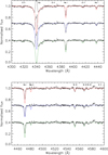 |
Fig. 10. Observed and theoretical profiles for selected wavelength regions (see Fig. 9 for details). |
| In the text | |
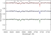 |
Fig. 11. Observed and theoretical profiles for selected wavelength regions (see Fig. 9 for details). |
| In the text | |
|
Fig. 12. Normalized Hα line profile from the X shooter spectra taken in 2017 December (red) and archival spectra from Evans et al. (2004) taken in 1999 September shown as solid blue lines. The emission line equivalent width increased by −16.1 Å within this period. We note that if the sky subtraction from the Evans et al. (2004) fibre spectra is poor, this difference will only be magnified. |
| In the text | |
|
Fig. 13. Left: near-infrared (J−H) vs. (H−K s) colour–colour diagram of known sgB[e] (open squares), warm hypergiants (open triangles), cBe stars (open circles), known S Doradus variables (blue dots), BSgs (small dots), and AzV 261 (red asterisk). Data taken from Humphreys et al. (2017a). The dashed red line is the main sequence locus at SMC metallicity. Right: mid-infrared [3.6 μm]–[4.5 μm] vs. [5.8 μm]–[8.0 μm] colour–colour diagram. Symbols are as in the left panel. The position of AzV 261 in both diagrams suggests the presence of free–free emission. The LBVs redward of colours [5.8 μm]–[8.0 μm] > 1.0 are contaminated by polycyclic aromatic hydrocarbon emission from nebulosity, with the regions of nebular contamination and dusty stars indicated following Humphreys et al. (2017a). |
| In the text | |
|
Fig. 14. Spectral energy distribution of AzV 261 covering photometry from the literature from U-8.0 μm. Overplotted as a solid line is the TLUSTY model atmosphere for the best-fit stellar parmeters of Teff = 18 000 K, log g = 2.5. The infrared-excess, corresponding to possible free-free emission of cold dust is best fit using a black-body model having Tb = 2550 K (shown as the dashed line). The dotted line is of constant frequency flux density normalized to the 3.6 μm photometry to make the free-free contribution clearer. |
| In the text | |
|
Fig. 15. Position of AzV 261 on the Hertzsprung–Russell diagram marked by the red asterisk, along the Bsgs studied here as grey squares. The positions of confirmed LBVs from the literature in the galaxy (black circles), LMC (blue circles), and the SMC (red circle) are also shown. Cyan circles mark the position of known LBVs in M31 and M33 (from Humphreys et al. 2017b). The dashed green lines are the stellar tracks from Brott et al. (2011) with the corresponding initial stellar mass indicated, and the solid line is the zero-age main sequence isochrone. |
| In the text | |
|
Fig. A.1. Light curves of 63 Bsgs that have data from the OGLE II survey. The Julian date is plotted against the measured I-band magnitude. |
| In the text | |
|
Fig. A.1. continued. |
| In the text | |
|
Fig. A.1. continued. |
| In the text | |
|
Fig. A.1. continued. |
| In the text | |
|
Fig. A.1. continued. |
| In the text | |
|
Fig. A.1. continued. |
| In the text | |
|
Fig. A.1. continued. |
| In the text | |
|
Fig. A.1. continued. |
| In the text | |
|
Fig. A.1. continued. |
| In the text | |
|
Fig. A.1. continued. |
| In the text | |
|
Fig. A.1. continued. |
| In the text | |
|
Fig. B.1. Lomb–Scargle periodogram of 64 Bsgs. The period in days is plotted against the power. The red and blue lines respectively represent the 99% and 95% significance calculated from the Monte Carlo bootstrap simulations. |
| In the text | |
|
Fig. B.1. continued. |
| In the text | |
|
Fig. B.1. continued. |
| In the text | |
|
Fig. B.1. continued. |
| In the text | |
|
Fig. B.1. continued. |
| In the text | |
|
Fig. B.1. continued. |
| In the text | |
|
Fig. B.1. continued. |
| In the text | |
|
Fig. B.1. continued. |
| In the text | |
|
Fig. B.1. continued. |
| In the text | |
|
Fig. B.1. continued. |
| In the text | |
|
Fig. B.1. continued. |
| In the text | |
|
Fig. C.1. Two-dimensional histogram of the δm–δt plot of 64 Bsgs. The δm in mag is plotted against the δt in days, and the colour is indicative of the density of the histogram following the colourbar. |
| In the text | |
|
Fig. C.1. continued. |
| In the text | |
|
Fig. C.1. continued. |
| In the text | |
|
Fig. C.1. continued. |
| In the text | |
|
Fig. C.1. continued. |
| In the text | |
|
Fig. C.1. continued. |
| In the text | |
|
Fig. C.1. continued. |
| In the text | |
|
Fig. C.1. continued. |
| In the text | |
|
Fig. C.1. continued. |
| In the text | |
|
Fig. C.1. continued. |
| In the text | |
|
Fig. C.1. continued. |
| In the text | |
Current usage metrics show cumulative count of Article Views (full-text article views including HTML views, PDF and ePub downloads, according to the available data) and Abstracts Views on Vision4Press platform.
Data correspond to usage on the plateform after 2015. The current usage metrics is available 48-96 hours after online publication and is updated daily on week days.
Initial download of the metrics may take a while.