| Issue |
A&A
Volume 618, October 2018
|
|
|---|---|---|
| Article Number | A42 | |
| Number of page(s) | 20 | |
| Section | Planets and planetary systems | |
| DOI | https://doi.org/10.1051/0004-6361/201833312 | |
| Published online | 11 October 2018 | |
The TROY project
II. Multi-technique constraints on exotrojans in nine planetary systems★,★★,★★★
1
European Southern Observatory (ESO), Alonso de Cordova 3107,
Vitacura Casilla 19001,
Santiago
19, Chile
e-mail: This email address is being protected from spambots. You need JavaScript enabled to view it.
2
Physics Institute, Space Research and Planetary Sciences, Center for Space and Habitability – NCCR PlanetS, University of Bern,
Bern, Switzerland
3
Instituto de Astrofísica de Canarias (IAC),
38200
La Laguna,
Tenerife, Spain
4
Departmento Astrofísica, Universidad de La Laguna (ULL),
38206
La Laguna,
Tenerife, Spain
5
Sub-department of Astrophysics, Department of Physics, University of Oxford,
Oxford
OX1 3RH, UK
6
Instituto de Astrofísica e Ciências do Espaço, Universidade do Porto, CAUP,
Rua das Estrelas,
4150-762
Porto, Portugal
7
Leibniz-Institut für Astrophysik Potsdam,
An der Sternwarte 16,
14482
Potsdam, Germany
8
IMCCE, Observatoire de Paris – PSL Research University, UPMC University Paris 06, University Lille 1, CNRS,
77 Avenue Denfert-Rochereau,
75014
Paris, France
9
Department of Physics, University of Coimbra,
3004-516
Coimbra, Portugal
10
CIDMA, Departamento de Física, Universidade de Aveiro, Campus de Santiago,
3810-193
Aveiro, Portugal
11
Departamento de Física e Astronomia, Faculdade de Ciências, Universidade do Porto,
Porto, Portugal
12
Space Research Institute, Austrian Academy of Sciences,
Schmiedlstr. 6,
8042
Graz, Austria
13
ESO,
Karl Schwarzschild Strasse 2,
85748
Garching, Germany
14
Departmento de Astrofísica, Centro de Astrobiología (CSIC-INTA),
ESAC Campus 28692 Villanueva de la Cañada,
Madrid, Spain
Received:
26
April
2018
Accepted:
27
June
2018
Abstract
Context. Co-orbital bodies are the byproduct of planet formation and evolution, as we know from the solar system. Although planet-size co-orbitals do not exists in our planetary system, dynamical studies show that they can remain stable for long periods of time in the gravitational well of massive planets. Should they exist, their detection is feasible with the current instrumentation.
Aims. In this paper, we present new ground-based observations searching for these bodies co-orbiting with nine close-in (P < 5 days) planets, using various observing techniques. The combination of all of these techniques allows us to restrict the parameter space of any possible trojan in the system.
Methods. We used multi-technique observations, comprised of radial velocity, precision photometry, and transit timing variations, both newly acquired in the context of the TROY project and publicly available, to constrain the presence of planet-size trojans in the Lagrangian points of nine known exoplanets.
Results. We find no clear evidence of trojans in these nine systems through any of the techniques used down to the precision of the observations. However, this allows us to constrain the presence of any potential trojan in the system, especially in the trojan mass or radius vs. libration amplitude plane. In particular, we can set upper mass limits in the super-Earth mass regime for six of the studied systems.
Key words: planets and satellites: gaseous planets / planets and satellites: fundamental parameters / minor planets, asteroids: general / techniques: radial velocities / techniques: photometric
Based on observations collected at the Centro Astronómico Hispano Alemán (CAHA) at Calar Alto, operated jointly by the Max-Planck Institut für Astronomie and the Instituto de Astrofísica de Andalucía (CSIC).
Partly based on data obtained with the STELLA robotic telescopes in Tenerife, an AIP facility jointly operated by AIP and IAC.
Based on observations collected at the European Organisation for Astronomical Research in the Southern Hemisphere under ESO programs 297.C-5051, 098.C-0440(A), and 298.C-5009
© ESO 2018
1 Introduction
The development of state-of-the-art instrumentation and space-based facilities in recent decades has boosted the discovery of extrasolar planets up to several thousands of detections1. This plethora of discoveries has shown the wide diversity of intrinsic and orbital properties that planets can have. Exoplanet research is currently focused on deep understanding of planet composition, structure, and atmosphere, in parallel with the search for Earth analogs. From our own system, we know that extrasolar systems should also host other components that also played an important role in moulding the architecture and properties of the planets. In the solar system, moons and more recently trojans (e.g., Lucy mission; Levison et al. 2017) are targets for in situ exploration since they contain clues on the formation and early evolution of our planetary system (e.g., Morbidelli et al. 2005; Borisov et al. 2017).
Trojan bodies corotate with planets in a wide variety of orbital configurations. These orbit configurations are mainly tadpole, i.e., orbiting the gravity wells of the L4 and L5 Lagrangian points, and horseshoe, i.e., librating from L4 to L5 in a horseshoe-like orbit in the corotating frame (see, e.g., Laughlin & Chambers 2002). The formation of these bodies is still under debate and two main mechanisms are proposed. First, in the in situ formation scenario, these bodies would form in the Lagrangian points throughout multiple inelastic collisions between the remnant dust particles of the protoplanetary disk trapped in the gravitationally stable regions. Indeed, swarms of particles trapped in the Lagrangian points are common outcomes of the hydrodynamical simulations used to explain the features observed in transition disks with potentially forming planets (e.g., Laughlin et al. 2002; Fuente et al. 2017). Similar to the core accretion process, this trapped material could have grown to larger bodies from kilometer- to moon- or planet-size by particles and pebble collisions. Interestingly, Beaugé et al. (2007) demonstrated that co-orbital bodies up to six times the mass of Mars can be formed in these regions under certain conditions and remain in stable orbits. Another proposed mechanism is the capture of these bodies in the Lagrangian points of giant planets during their migration along the disk (see, e.g., Namouni & Morais 2017). This would allow larger bodies to be trapped in these regions. Each of these mechanisms, occurring during the first stages of planet formation and evolution processes, have different imprints in the physical and orbital properties of the co-orbitals. Hence, co-orbital bodies contain primordial information about these first stages of the system. Consequently, the study of trojans in the solar system and the search for trojans in extrasolar systems (and minor bodies in general; Lillo-Box et al. 2018b) is key to understanding the whole picture of the properties of planetary systems. In particular these objects can provide significant insight into the nature of formation processes by allowing us to understand if some exoplanetary properties, such as the presence of hot Jupiters, are a product of nature (formation) or nurture (evolution).
Previous works have developed various techniques to search for these bodies but none has been found yet. Several techniques have been explored, namely, radial velocity (Ford & Gaudi 2006; Leleu et al. 2015, 2017), transits (Janson 2013; Hippke & Angerhausen 2015), or transit timing variations of the planet (Ford & Holman 2007; Madhusudhan & Winn 2009; Schwarz et al. 2015). In Lillo-Box et al. (2018a), we presented the TROY project, a multi-technique effort to detect the first bodies co-orbiting to known extrasolar planets. We analyzed a combination of radial velocity and transit data with the methodology described in Leleu et al. (2017), which is a generalization of the Ford & Gaudi (2006) technique, expanding the parameter space to horseshoe and large amplitude tadpole orbits. We used archive radial velocity data together with Kepler and ground-based light curves to constrain exotrojan masses in 46 single-planet systems in short-period orbits (P < 5 days). We did not find significant evidence of trojan bodies in any of the studied systems, but we were able to place upper limits to masses in both Lagrangian points and start populating the parameter space toward a definition of the trojan occurrence rate at various mass regimes. For instance, we discarded Jupiter-mass (or more massive) trojans in 90% of the systems, which might indicate difficulties in forming, capturing, or keeping trojans in stable orbits during the inward migration of the planet (as theoretically predicted in, e.g., Rodríguez et al. 2013).
Some of the systems studied in Lillo-Box et al. (2018a) showed hints of a mass imbalance between the two Lagrangian points at the 2σ level. Even though they were not significant detections, they certainly deserve additional follow up. In this paper, we present an extensive amount of dedicated radial velocity and light curve data of nine of these systems to look for the planet-mass co-orbital candidates found in our previous work. In Sect. 2, we describe the multi-technique observations and data reduction. In Sect. 3, we present the method followed to constrain the different regions of the parameter space to restrict the possible presence of trojan planets in these systems; and Sect. 4 presents the results for each individual system. In Sect. 5, we discuss these results. In Appendices A and B we show large figures and long tables, respectively.
2 Observations
We have used several data sets from previous publications as well as newly acquired data. In this section, we summarize these observations and briefly describe the target sample.
2.1 Target sample
Nine systems were selected for further follow up from our radial velocity analysis in Lillo-Box et al. (2018a) because these systems presented hints of some mass imbalance between the two Lagrangian points. The selected systems are shown in the first column of Table 1. The planets in all nine systems studied in this work have been confirmed and characterized through both transits and radial velocity observations. Among these systems, seven are gas giants with masses above one Jupiter mass, HAT-P-12 b is a Saturn-mass planet, and GJ 3470 b is a 13.7 M⊕ planet. All of these systems transit main-sequence stars of spectral types FGK (and M in the case of GJ 3470) with orbital periods below 3.5 days.
2.2 Radial velocity
We used thearchive radial velocity data presented in Lillo-Box et al. (2018a) and newly acquired high-resolution spectra from HARPS (Mayor et al. 2003), HARPS-N (Cosentino et al. 2012), and CARMENES (Quirrenbach et al. 2014). In Table 1 we present a summary of the new radial velocity observations obtained for each of the nine systems, distinguishing between archive and new observations.
All three instruments are high-resolution fiber-fed échelle spectrographs with resolving powers R = 120 000 (HARPS, 3.6 m telescope at La Silla Observatory, ESO, Chile), R = 120 000 (HARPS-N, Telescopio Nationale di Galileo, La Palma, Spain), and R = 81 200 (CARMENES, 3.5 m telescope at Calar Alto Observatory, Almería, Spain). These instruments are all located in temperatureand pressure controlled vacuum vessels inside isolated chambers to improve their stability. Also, all three instruments are equipped with a second fiber for simultaneous wavelength calibration. In the case of HARPS-N and CARMENES, we fed the second fiber with a Fabry–Pérot, while HARPS was fed by a simultaneous ThAr lamp.
In the case of HARPS and HARPS-N, the data were reduced using the corresponding pipelines available at each observatory. In both cases, the pipeline also determines precise radial velocities using the cross-correlation function method (CCF; Baranne et al. 1996; Pepe et al. 2002) with a binary template of a similar spectral type as the target star. In the case of CARMENES, we used the CARACAL pipeline (Caballero et al. 2016) to perform the basic reduction, wavelength calibration, and extraction of the spectra. Then, we used our own code carmeneX, partly based on the SERVAL pipeline (Zechmeister et al. 2018)2, to compute the radial velocities using the CCF technique with a solar-type binary mask with more than 3000 spectral lines (adapted form the mask developed for CAFE; see Aceituno et al. 2013 and Lillo-Box et al. 2015).
We used HARPS in a five-night campaign3 on 21–25 January 2017 that was unfortunately affected by poor weather conditions, and only allowed us to use 1.5 nights owing to high humidity, and in a monitoring campaign4 in which we gathered 13 data points for WASP-5 over four months. In the case of HARPS-N, we had a three-night run5 on 6–8 February 2017 with successful observations during the whole campaign. Finally, we used CARMENES in a four-night run6 on 28–31 January 2017 with a success rate of 60%, mostly owing to thick clouds and high humidity, and in another four-night run on 12–15 December 20177 with a 48% success rate. In Tables B.1–B.7, we show the derived radial velocities and their uncertainties for the new radial velocity observations.
Summary of the data used in this paper for the nine targets analyzed, including the number of data points for each technique, both new (Nnew) and from archive data (Narch).
2.3 Differential photometry
We used CAFOS (Meisenheimer 1994) at the 2.2 m telescope in Calar Alto Observatory, WiFSIP at the STELLA1 1.2 m robotic telescope (Strassmeier et al. 2010) of the Teide Observatory (Tenerife, Spain), and FORS2 (Appenzeller & Rupprecht 1992) at the Very Large Telescope (VLT; Paranal Observatory, ESO, Chile) to photometrically explore the regions around one of the Lagrangian points of the exoplanets studied in this work. The selection of the particular Lagrangian region (either L4 or L5) was carried out on the basis of previous radial velocity analysis in Lillo-Box et al. (2018a) for most of the targets. In Table B.8, we present the detailed characteristics of these observations for each of the targets. In all cases, the small eccentricities of the planets allow us to compute the transit times of the Lagrangian points as T0,LP = T0 ± 1∕6 × P, where T0 is the planet mid-transit time, P is the orbital period, and the plus (minus) sign represents the L5 (L4) location. Based on this, we used the orbital properties from NASA Exoplanet Archive to compute the transit times using the Transit Ephemeris Service8 at the corresponding location and custom phase. Since the radial velocity analysis is not sensitive to possible librations, the wider range of time we can observe around the Lagrangian point the better we can constrain the parameter space.
We used CAFOS in imaging mode9 to obtain high-cadence relative photometry of eight of the targets. The field of view is reduced down to 7 × 7 arcmin (i.e., around 800 × 800 pixels for a plate scale of 0.53 arcsec/pix) to decrease the readout time and thus increase the observational cadence. The exposure times for each target depend on their magnitudes and atmospheric conditions, ranging between 10 and 30 s in the SDSS i filter. The total time span for the observations is typically four hours centered on the Lagrangian point midpassage. We slightly defocused the telescope to increase the signal-to-noise ratio of the source, reaching an average of 50 000 counts per pixel. In the case of HAT-P-20, we defocused the telescope (both in CAFOS and WiFSIP observations) just up to 2 arcsec to avoid contamination from a close companion at 6.2 arcsec (Bakos et al. 2011). On the contrary, for WASP-77, we strongly defocused the telescope (up to donut-shaped point spread function) to merge the light from a close companion at 3 arcsec (Maxted et al. 2013) and thereby avoiding flux fluctuations inside the aperture due to possible seeing variations along the observation.
The CAFOS photometry was reduced with a custom aperture photometry pipeline10. The pipeline applies first the basic data reduction steps of bias subtraction and flat-field division, after which it calculates the aperture photometry for the target star and a set of potential comparison stars using five aperture sizes. The final relative light curve is generated by finding a combination of comparison stars and aperture sizes that minimizes the relative light curve point-to-point scatter. A slightly modified version of the pipeline is used when the target star is accompanied by a bright nearby star (close enough for the PSFs to blend). In this case the photometry is calculated for a set of circular apertures and a set of elliptical apertures that contain the target and contaminant. We calculate the relative target-contaminant flux based on the frames with best seeing, remove the fractional contaminant flux from the combined flux, and use the circular aperture photometry centered on the target and contaminant to test that the contaminant is stable.
We also used WiFSIP to explore the Lagrangian points of three exoplanets11. The WiFSIP field of view is 22 × 22 arcmin and the plate scale corresponds to 0.322 arcsec/pix. In this case, given the robotic nature of the telescope and in order to increase the execution probability of the program, we asked observations of three times three hours around the Lagrangian point mid-transit time, starting at random phases between two hours and half an hour before the start of the expected transit. The typical exposure times range between 10 and 80 s in the SDSSr band. In the same way as explained before, we also defocused the telescope forsome targets in order to reach the maximum precision possible. The data were reduced with the software tools used previously for high-precision exoplanet transit photometry with STELLA/WiFSIP (e.g., Mallonn et al. 2016). Bias and flat-field correction was carried out with the standard STELLA pipeline. For aperture photometry we employed the publicly available tool SExtractor (Bertin & Arnouts 1996). Our software tools choose the selection of reference stars that minimize the standard deviation in the light curves and, by the same criterion, also choose the best aperture size.
Finally, we also used FORS2 on 2016-10-26 in imaging mode with the z_SPECIAL filter to explore the L5 region of WASP-5b during 3.68 h12. An individual exposure of 12 s was set, providing photon-noise limited images without need to defocus the telescope13. The FORS2 data was reduced and extracted following the same principles described above for the CAFOS data, using a similar (adapted) pipeline.
In all cases, regardless of the instrument used, the extraction procedure gathers a set of covariates (airmass, median sky level, full width at half maximum, and centroid shift of the target) that are used next to detrend the light curve (see Sect. 3.2.1).
2.4 Transit timing variations
We collected the transit times of all targets studied in this paper through the Exoplanet Transit Database (ETD; Poddaný et al. 2010). We only used transit epochs with data quality better or equal than 3, as flagged in the ETD. In the last two columns of Table 1, we show the number of epochs for each target together with the corresponding references.
3 Methodology: constraining the parameter space
We use all the above described data to constrain the parameter space of a potential co-orbital planet. While the combination of the radial velocity and planet transit data (Sect. 3.1) can constrain the mass of the trojan (see Leleu et al. 2017; Lillo-Box et al. 2018a), the dedicated multi-epoch photometric exploration of the Lagrangian points (Sect. 3.2) and the measured transit timing variations of the planet (Sect. 3.3) can constrain other regions of the parameter space characterizing the co-orbital and its orbit. We explain each of these approaches in the following.
3.1 Radial velocity and planet transit
In all cases where new radial velocity (RV) data from our own monitoring campaigns or from public data are available, we apply the same technique as in Lillo-Box et al. (2018a) based on the theoretical approach described inLeleu et al. (2017) to obtain an upper limit to the mass of the trojan and to decide on the Lagrangian point to be explored photometrically. This analysis is based on the determination of the α parameter, which corresponds to mt∕mp sinζ to first order in eccentricity, where mt is the mass of the trojan, mp is the mass of the planet, and ζ is the resonant angle representing the difference between the mean longitudes of the trojan and the planet. If α is significantly different from 0, the system is hence a strong candidate to harbor co-orbitals. Consequently, for a known planetary mass and an assumed resonant angle, an upper limit on α can be directly translated into an upper limit for the mass of trojans at the Lagrangian points. We then obtain  as the maximum mass (95% confidence level) that a potential trojan could have on the average location of the co-orbital along the observation time span.
We followed the same procedure as in our previous work, modeling the radial velocity with the equation described inLeleu et al. (2017) and including a Gaussian process to account for the presence of active regions in the stellar surface that can lead to correlated noise in the data. To this end we used a quasi-periodic kernel (described in Faria et al. 2016). We set Gaussian priors for the orbital period, time of mid-transit of the planet, and c ≈ ecosω when this parameter can be constrained from the detection of the secondary eclipse. These priors are centered on the values from the literature and we set a width equal to three times the estimated uncertainties provided in the literature. Log-uniform priors are set to the GP hyperparameters and uniform priors are used for the rest of the parameters, including the systemic velocity (Vsys), radial velocity semi-amplitude (K), α, and d ≈ esinω. The results of the radial velocity fitting are shown in Fig. A.1 and the median and 68.7% confidence values of the main fitted parameters are shown in Table 2, and are discussed individually in Sect. 4. Also, in Fig. 1, we compare the α values for these nine systems between the current work and our first analysis in Lillo-Box et al. (2018a). The main conclusion is that we can reduce the uncertainty in systems for which a significant amount of new data points were obtained compared to the previous data. This allows us to set lower upper mass limits. For instance, in the case of HAT-P-36 and WASP-77A, the α parameter is now compatible with null within 1σ.
3.2 Photometric exploration of the Lagrangian points
The photometric exploration of the Lagrangian points can constrain, first, the trojan size, if we assume small librations around the Lagrangian point; and second, the orbital parameters of the co-orbital body, especially the libration amplitude assuming coplanarity. In the following section, we describe the different analyses of the precise photometry obtained during our ground-based campaigns. Each subsection focuses on particular aspects, namely, individual transit searches on each epoch assuming coplanarity and hence a similar transit duration as the planet (Sect. 3.2.1), the implications of non-detection on the trojan libration amplitude (Sect. 3.2.2), and transit search on the combined light curve assuming no libration (Sect. 3.2.3).
Derived parameters for the nine planetary systems analyzed.
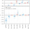 |
Fig. 1 Comparison between the α values obtained with the new data (circles) and the values published in Lillo-Box et al. (2018a). The colored dotted lines represent the 3σ uncertainties. The blue colors indicate α ± σ > 0 (i.e., candidate) and red colors indicate α − σ < 0 < α + σ (i.e., no detection). Top panel: close view of the region around α = 0 |
3.2.1 Individual epochs (coplanar case): search for transits
We used different epochs of a single system independently to look for transits in the observed time spans. The search is performed through transit fitting of the light curve, which also allows us to estimate the maximum object size in case no transit is detected. This fit is carried out using the batman14 python module (Kreidberg 2015), in which we assume a Gaussian prior on the orbital period (P), semimajor axis to stellar radius (a∕R⋆), and inclination (i) parameters. This implies that we are looking for coplanar (or very close to coplanar) trojans, thus having transit durations similar to that of the planet. But we note that not completely fixing these values still allows for some freedom in the trojan transit duration. We then leave the mid-transit time of the trojan (T0,t), the trojan-to-stellar radius (Rt ∕R⋆), zero level (out-of-transit flux level, F0), and a photometric jitter to account for white noise (σjit) as free parameters with uniform priors. The specific priors and ranges are shown in Table 3. We also include a baseline model simultaneously to account for possible correlations with airmass (χ), seeing (s, full width at half maximum of the target point spread function), time (t), position of the target on the detector (xy), and background (b). In a first stage, we use linear dependencies for these parameters,  . Mathematically, the baseline model can be represented as
  , where ai are the coefficients to be determined and pi are each of the parameters described above. The baseline and transit models are fitted simultaneously, assuming that each data point is a realization of
  .
.
We use emcee15 (Foreman-Mackey et al. 2013) with 50 walkers and 50 000 steps per walker to explore the posterior distribution of the transit parameters and baseline coefficients. We use the last half of each chain to compute the final posterior distributions and parameter–parameter dependencies. We test a model with trojan (trojan hypothesis) and without trojan (null hypothesis). In the latter case, the number of free parameters reduces to F0, σjit, and the baseline parameters. The Bayesian evidence (E) of these two models are estimated using the perrakis code16. Based on this Bayesian evidence, we can estimate the Bayes factor (BF) between the two models as the ratio of the evidence of the trojan hypothesis (Et) to the null hypothesis (E0), such that BF = lnEt − lnE0. A positive BF would favor the trojan hypothesis against the null hypothesis, with BF > 6 considered as a strong evidence.
Additionally, the posterior distribution of the trojan-to-star radius ratio (Rt ∕R⋆) is checked. If this parameter is significantly different from zero (i.e., the median value is larger than the 95% confidence interval) and the Bayes factorfavors the trojan hypothesis against the null hypothesis, then we consider that we have a candidate trojan transit. In this case, we proceed by testing models (both with and without trojan) with quadratic dependencies for the baseline parameters, p(t2) + p(χ2) + p(s2) + p(xy2) + p(b2). More specifically, we first run all parameters with quadratic dependencies, then we check the relevant parameters producing significant non-zero coefficients in the fit and we finally run a last model only including those relevant parameters. We then re-estimate the Bayesian evidence and look for the model with the largest evidence. If that model corresponds to a trojan-hypothesis model and keeps the significance of the Rt ∕R⋆ parameter, then we consider the transit as a strong trojan transit candidate.
In the cases in which no significant transit was detected, we can determine a maximum radius of the trojan per each epoch ( ). This is determined as the 95% confidence interval of the posterior distribution of the Rt ∕R⋆ parameter. We also establish a time interval (which can be translated to a phase interval) in which we can assure that there is no transit of a body larger than
  (see Table B.9). This time interval is considered as the entire observing window, which implies that we only consider a transit detection if we have more than half of the transit. We note that this is a conservative assumption for constraining the parameter space. An example of this approach is shown in Fig. 2 for the transit of the L5 Lagrangian point of HAT-P-36 b observed with CAFOS. The figure shows the modeling with the null hypothesis and the detectable limit by these observations in the bottom panel (dashed horizontal line). In Fig. A.2, we show for all nine systems the results of the null-hypothesis models once the fitted baseline contribution has been removed.
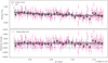 |
Fig. 2 Example of the light curve analysis of the L5 region of HAT-P-36 b (observed with CAFOS on 2018-03-22) including the linear baseline model (see Sect. 3.2.1). Top panel: raw light curve (violet symbols) together with the 15 min binned data (black open circles, for visualization purposes) and the baseline model fitted. In this case, we assume to trojan (null hypothesis). Bottom panel: baseline-corrected light curve with the detectable limit calculated as the 95% interval for the Rt ∕R⋆ parameter in the trojan model. In both panels, the shaded regions correspond to the 68.7% and 99.7% confidence intervals. |
Priors for the light curve analysis and transit fitting.
3.2.2 Individual epochs (coplanar case): parameter space constraint
We can then use the time range of non-detected transit for each epoch to constrain the parameter space of the trojan orbit. We can do this by determining the parameter range where the trojan would not transit during these time ranges (assuming the trojan is larger than the above estimated maximum radius). To this end, we apply a Monte Carlo Markov chain (MCMC) using a modified likelihood function ( ) that increases toward the edges of the observed time ranges and is flat and maximum outside of these ranges, i.e.,
 (1)
(1)
where
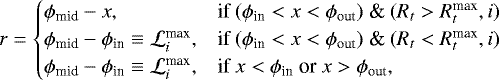 (2)
(2)
where ϕin and ϕout are the orbital phases corresponding to the earliest and latest edge of the time range (i.e., tin and tout). The value ϕmid represents the mid-time of this time range and σ is one-fourth of this time span. Consequently, the likelihood is minimum at the mid-time of the observations and is maximum and constant outside of this range. The total likelihood ( ) is the sum of the likelihoods (
 ) calculated as above for each transit epoch observed.
The model calculates the expected time (or orbital phase) of the mid-transit based on the projected position of the trojan in the sky, which can be simplified from Eqs. (53)–(55) in Murray & Correia (2010) for small eccentricities as
![Mathematical equation: \begin{eqnarray*} &X_t = & a/R_{\star}\Big[\cos{\lambda_t} + e_t/2 \Big(-3\cos{\omega_t} + \cos(2\lambda_t-\omega_t)\Big) \Big]\nonumber \\ &Y_t = & a/R_{\star}\Big[\sin{\lambda_t} + e_t/2 \Big(-3\sin{\omega_t} + \sin(2\lambda_t-\omega_t)\Big) \Big]\cos{i} \nonumber\\ &Z_t = & a/R_{\star}\Big[\sin{\lambda_t} + e_t/2 \Big(-3\sin{\omega_t} + \sin(2\lambda_t-\omega_t)\Big) \Big]\sin{i}, \end{eqnarray*}](/articles/aa/full_html/2018/10/aa33312-18/aa33312-18-eq12.png) (3)
(3)
where et and ωt are the trojan eccentricity and argument of the periastron; λt is the mean longitude of the trojan; i is the orbital inclination; and a∕R⋆ is the semimajor axis to stellar radius ratio. Based on these equations and the reference frame described in Leleu et al. (2017), the trojan transit occurs when Xt = 0 (conjunction), |Yt |< 1 (the object transits the star), and Zt < 0 (primary eclipse). Hence, we can calculate the times at which these conditions are fulfilled (i.e., the mid-times of the trojan transit on each orbit) and, in particular, at the orbits that we observed.
By comparing these values with the time ranges for each epoch we can constrain the parameter space of theparameters involved so that transits do not occur during these time ranges. To that end, we use 20 walkers with 50 000 steps per walker in our MCMC and we only select the steps with  equal to the sum of the maximum likelihoods on each epoch, i.e.,
  . With these selected steps (usually around 80% of the original chain) we can then construct the corner plot diagram with the parameter–parameter dependencies of the orbital models not having trojan transits during the observed time ranges. This diagram provides theconstraints of the parameter values based on the observed photometric data in the absence of trojan transits and can be used, for instance, to provide a minimum libration amplitude for the trojan. In case several epochs were observed, we include the possibility of an eccentric orbit for the trojan. In case only one epoch is available, we assume circular orbit for the trojan (et = 0).
As an example, we show in Fig. 3 the results for the analysis of WASP-77A. The red vertical lines represent the orbital phase interval that we observed, finding no transits. The expected transit is indicated by the horizontal lines; the dotted line is the expected ingress and egress phases. The colored lines represent a sample of accepted models from the whole MCMC chain. For a model to be accepted it has to either not cross the red lines if the trial trojan radius is larger than the light curve detectability limit (blue colored lines), or if the trojan transits during our observations but it is smaller than the detectability limit (green lines). In this particular example, our data allows us to reject trojans larger than 4 R⊕ with librations amplitudes shorter than 25°.
3.2.3 Combined epochs
Finally, we can also combine all epochs for the same object and Lagrangian point by assuming that the would-be transits are achromatic, given that we observed with different filters on different telescopes. This provides a smaller maximum radius of the trojan in case of no libration or in the case that the libration period is much larger than the time span of the observations. To do this we remove the median baseline model for each epoch in the null hypothesis and then combine all epochs in orbital phase (see Fig. 4). We now try to search for a transit in this combined light curve to get a maximum radius for a stationary trojan (i.e., with no libration). To this end we follow the same procedure as in Sect. 3.2.1.
We can translate the maximum trojan radius into a maximum trojan mass using the forecaster module (Chen & Kipping 2017). According to the documentation of this module, it provides accurate estimates of the masses in the case of terrestrial and Neptune-like worlds, which are the typical cases for the radius limits found in this paper.
3.3 Transit timing variations
As presented in Ford & Holman (2007), the amplitude of the variations in the transit times of the hosting planet (Ktt) due to the libration of a trojan with amplitude17 Kζ are well represented by the Eq. (1) in that paper, i.e.,
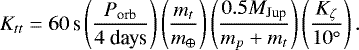 (4)
(4)
If no periodic variations are found, we can estimate an upper limit for this amplitude by simply fitting a sinusoidal function to the measured transit timing variations (TTVs), with amplitude Ktt. This way, we can find a direct relation between the trojan mass and libration amplitude, thus constraining this parameter space. We can compute the maximum TTV amplitude (Ktt,max) as the 95% confidence level from the marginalized posterior probability of Ktt. In tadpole low eccentricity orbits, we expect the libration of the trojan to introduce sinusoid-like variations in the time of transit of the planet. Hence, under this assumption, we can use the simple model Z + Ktt sin(νlibt + ϕtt), where νlib is the libration frequency (Leleu et al. 2015), ϕtt a phase offset, and Z a zero level to account for the uncertainties in the orbital period and mean mid-transit time. We assume a uniform prior for all parameters involved in the model, with 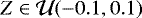 h,
h, 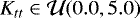 h,
h,  with
with  , and
, and  .
.
In order to sample the posterior distribution we use an MCMC algorithm by means of the emcee code. We use 50 walkers and 100 000 steps per walker. We remove the first half of the steps and compute the marginalized posterior distribution for the Ktt parameter. We check that the posterior distribution is actually truncated at Ktt = 0 (i.e., no detection of periodic TTVs). Then, the 95% percentile is computed to obtain Ktt,max. Given this value, we can get a contour in the mt(Kζ) function to constrain the parameter space.
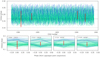 |
Fig. 3 Example of the analysis of the parameter space constrain based on the non-detection of transits in our data for the system WASP-77A. Top panel: orbit number (X-axis) vs. the orbital phase covered by our observations (red vertical lines). The transit of the Lagrangian point (L5 in this case) is expected to happen between the dotted horizontal lines. The colored lines represent a small sample of the accepted models. For a model to be accepted it has to either not cross the red lines if the trial trojan radius is larger than the light curve detectability limit (blue lines) or if the trojan transits during our observations but is smaller than the detectability limit (green lines). The bottom panels are just close views on each of the four epochs, where the X-axis is the phase from the Lagrangian point conjunction. |
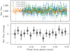 |
Fig. 4 Example of the light curve combination in phase for the case of WASP-77A. The individual epochs are shown in the top panel (after removing the linear baseline model) and the combined light curve is shown in the bottom panel; 10 min bins have 225 ppm rms. The vertical dotted lines indicate the expected transit ingress and egress of the Lagrangian point. |
3.4 Constraints to the trojan mass vs. libration amplitude parameter space
The analysis described above for the the multi-technique data produces a variety of constraints on several planes of the parameter space. One interesting plane is the trojan mass vs. the libration amplitude because it provides both physical and dynamical information relevant for detection purposes. In Fig. 5, we show an example of the constraints provided by our analysis on this plane assuming coplanarity between the trojan and planet orbital planes. The analysis of the radial velocity provided in Sect. 3.1 constraints the mass of the trojan regardless of the libration amplitude, since the data was taken during a long time span (much longer than the libration period). This is shown by the red shaded region in the example Fig. 5. In order to translate the results from the light curve analysis (from the individual analysis in Sect. 3.2.1, the dynamical analysis combining the individual epochs in Sect. 3.2.2, and from the combined light curve in Sect. 3.2.3), we convert the maximum trojan radius to maximum trojan masses using the forecaster module (Chen & Kipping 2017). The libration parameter in this case is constrained by the time range of our observations in the case of individual light curves and from the expected transit duration for the combined light curves. Finally, the TTVs can constrain this parameter space as already described in Sect. 3.3 (shown in green in the example Fig. 5). The diagram corresponding to each of the nine systems can be found in Fig. A.3.
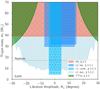 |
Fig. 5 Detailed example of the constraining of the trojan mass vs. libration amplitude parameter space in the case of WASP-77A.Negative (positive) values for the libration amplitude are used to represent constraints on transits before (after) the Lagrangian point passage. Only the white region is not explored by our data. |
4 Results per system
Based on the analysis of the multi-technique data presented in Sect. 3, we can now constrain the presence of co-orbital bodies in the surroundings of the Lagrangian points in these nine systems. We summarize the results for each of the analyzed planetary systems in the following.
4.1 GJ 3470
Only one Lagrangian transit is available for this system. The analysis of the light curve shows no significant detection of any transit up to 3.7 R⊕. The analysis of the radial velocity data provides a value for the α parameter significantly different from zero. However, the eccentricity fitted is too large and thus the radial velocity equations are out of the validity range (i.e., e < 0.1). Consequently, the result is degenerate and we can neither discard the trojan scenario nor confirm it. In order to solve this dichotomy, a measurement of the secondary eclipse of the planet would be needed18 together with the development of new equations with a wider eccentricity validity range. Also, the TTVs do not show a significant periodic variation up to 3.2 min. This allows us to put important constraints on the mass of any potential librating trojan and confirms that should it exist with a moon- or planet-size, the libration amplitude should be smaller than 4° for trojans with masses larger than Earth and smaller than 10° for sub-Earth-mass trojans.
4.2 HAT-P-12
The photometric exploration of L4 in HAT-P-12 did not show any significant dimming down to 4.8 R⊕. However, only half of the Lagrangian point passage could be covered with CAFOS owing to bad weather conditions. The radial velocity analysis provides α = −0.141 ± 0.082, corresponding to a trojan mass of 10.8 ± 6.3 M⊕ at L4. This sets an upper limit of 21 M⊕ in L4 and rejects any trojan more massive than 4 MMoon at L5. The TTVs in this system restrict the libration amplitude importantly, leaving only sub-Earth masses to libration amplitudes larger than ~ 7°. Hence, if larger bodies are present in this Lagrangian point, low libration amplitudes are expected and so sub-mmag precision light curves could explore this regime (an Earth-size body would induce ~170 ppm transit depth in this system). This system illustrates that since TTVs are proportional to the trojan-to-planet mass, small co-orbitals should be more easily found corotating with low mass planets.
4.3 HAT-P-20
The large amount of radial velocity data that we gathered for HAT-P-20 b added to the archive spectra allows us now to estimate α = 0.0017 ± 0.0048. This very small value allows us to set an upper limit on the mass of any potential trojan of 25 M⊕. The TTVs do not show any clear periodic sinusoidal signal. However, the data show peak-to-peak variations up to 2.5 min.
A total of three observations of the L5 transit passage have been observed with CAFOS for this target. The quality of the observations is very variable, going from very bad quality (on 2017-04-03 with flux variations up to 5 mmag) to very good quality data at the ~1.5 mmag level on individual measurements. We tested the null hypothesis and the trojan hypothesis in all three epochs. Theresults show that for two epochs (2017-04-03 and 2017-11-16) the null hypothesis has significantly larger evidence than the trojan hypothesis. Both epochs allow us to set upper limits on the trojan size of 8.3 R⊕ and 2.9 R⊕ (respectively) in the phases covered by these epochs.
However, the results on the night of 2017-12-09 provide larger evidence in favor of the trojan model against the null hypothesis, showing a Bayes factor of 12 toward the trojan model. These two models (with and without trojan) are built on the basis of linear dependencies with the baseline parameters. We also tested various quadratic dependencies for the null hypothesis but all of these show Bayes factors even more in favor of the trojan linear-baseline model. This favored model reveals a dimming in the light curve at phase 0.195, which would correspond to a 5.8 R⊕ object. In Fig. 6, we show the CAFOS light curve with the baseline model removed and the median fitted transit model. Despite the large significance of the trojan model, the large radius of the possible co-orbital is puzzling (although it could also be a compact trojan swarm). Also, the baseline models without trojan are able to reproduce the would-be ingress qualitatively well, removing the transit signal. In Fig. A.2 (in the panel labeled as “HAT-P-20 - 171209”), this non-trojan model is shown.
As easily pointed out in both figures, at phases larger than 0.20 there is a clear modulation that any baseline model fails to reproduce. In order to test if this might be the only reason why the trojan model is favored against the non-trojan model we performed the same analysis by removing all data points after phase ϕ >0.20 (after Juliandate 2458097.2121). The results of this analysis, however, increase the significance of the non-trojan model providing an evidence 12 times larger now in favor of the null hypothesis. We then conclude that the strong modulation at the end of our observationsstrongly affects the result of the analysis and so we cannot reach a conclusion concerning the presence of any large body in thistransit with the current data. Since this deep event (that would correspond to a gas giant) is not seen neither in the other epochs nor in the radial velocity data, we assume for the subsequent discussion that no trojan is present in this system.
Under this assumption, the analysis of the combined light curve produces an upper limit on the trojan mass of 2 R⊕ at the exact Lagrangian point.
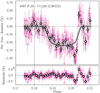 |
Fig. 6 Trojan hypothesis model after removing the linear baseline model for HAT-P-20. This trojan model is only favored against the null hypothesis if we include the whole data set. However by removing the feature at phases ϕ > 0.20, the null hypothesis is favored. The black shaded vertical line represents the expected egress of the Lagrangian point, showing thelarge time lag of the would-be trojan transit. This light curve corresponds to the data from CAFOS at CAHA on 2017-12-09. |
4.4 HAT-P-23
In the case of HAT-P-23, we found α = −0.132 ± 0.082, corresponding to a 95% upper limit of 205 M⊕. We photometrically explored the L4 region during three different passages of this region in front of its star. We can discard coplanar transits in these observations of objects up to 5.1−6.2 R⊕. Furthermore, the combined light curve allows us to discard bodies larger than 1.39 R⊕ that lay exactly at the Lagrangian point (or experiencing very small librations). The analysis of the parameter space of the trojan properties that still remain plausible despite the non-transit detection, just leaves the possibility of large libration amplitudes for circular orbits of the trojan, which are avoided by the lack of TTV modulations. Hence, should it exist, the trojan co-orbiting to HAT-P-23 b must be either a planet smaller than Neptune with a large libration amplitude or a low mass (< 4 M⊕) planet in a low libration amplitude but highly eccentric orbit.
4.5 HAT-P-36
Photometric variability at the 1.5 mmag level appears in the CAFOS and WiFSIP light curves around the L5 region, which might be due to the moderate activity of the host star (log R′ = −4.65 dex; Mancini et al. 2016). No significant dimming is detected down to 6 R⊕ at L5 in the CAFOS light curve; the WiFSIP data are of slightly worse quality in this case. The new radial velocity measurements presented in this paper allow us now to decrease the α parameter to 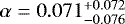 (from the previous
  ), thus they are now fully compatible with no trojan at the 1σ level. This now corresponds to a maximum mass of the trojan of 128 M⊕ at L5 (around four times smaller than our previous upper limit) and 38 M⊕ at L4. However, the combination of all three available transit observations allows us to set small upper radius of 2 R⊕ to any trojan body located at the exact Lagrangian point.
4.6 WASP-2
In this case we find 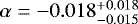 , so that we can set an upper limit to the trojan mass of 15.1 M⊕, similar to our previous measurement. The analysis of the TTVs also do not show any significant periodic variation and the single transit we could observe with CAFOS do not show any significant dimming. The upper limit that we can impose based on this non-detection of the transit is 4.3 R⊕. The TTVs also indicate that trojans more massive than the Earth should have libration amplitudes smaller than 25°.
4.7 WASP-36
The 14 new radial velocity measurements obtained for this target with HARPS-N and CARMENES allows as to decrease the significance in the α parameter with respect to Lillo-Box et al. (2018a). We find now α = 0.031 ± 0.028 (compared to the previous 0.092 ± 0.043). We have now decreased by two the uncertainty in this parameter. However, because of the large mass of the planet, we can only set an upper limit to its trojan mass at L5 of mt < 63 M⊕ (compared to the previous 146 M⊕). Additionally, the TTVs do not show variations larger than 320 s. Finally, the two WiFSIP observations of the Lagrangian transit do not show any dimming down to 8 R⊕ and 5.4 R⊕, respectively.The combined light curve, however, provides a much smaller upper limit to the size of any potential trojan of 2.1 R⊕. This allows us to reject any possible trojan with mt > 10 M⊕ at the exact position of the Lagrangian point.
4.8 WASP-5
The new radial velocity analysis presented in this work (including new HARPS data) now provides α =0.002 ± 0.010, corresponding to an upper limit of 10.4 M⊕ at L5 and 7.6 M⊕ at L4. The periodogram of the TTVs in this case shows a peak around 18 days although this peak is not statistically significant. The modeling of the TTVs consistently provides a possible periodic solution with an amplitude of Ktt = 32 ± 18 s and a periodicity of  days. If we neglect the mass of the trojan, the expected libration period would be 15.7 days in this system. But, this periodicity can be elongated owing to different factors such as mutual inclination or eccentricity.
Using Eq. (1) in Ford & Holman (2007) we can use the estimated Ktt to get a relation between the trojan mass and the libration amplitude. Given the upper limit on the mass provided by the radial velocity analysis, and assuming the TTV modulations, the possible trojan should have a minimum libration amplitude of 4°. The lower the trojan mass the larger libration amplitude is needed to produce the observed TTV modulation.
Such low libration amplitude implies that the trojan could transit the star very close to the Lagrangian point passage on every orbit. The upper mass limit of 10.4 M⊕ provided by the radial velocity would correspond to an object of  R⊕. Our FORS2 observations of the L5 passage do not show any statistically significant dimming, providing an upper limit on the trojan radius of 4.5 R⊕. Hence, we would need at least two more transits to test the regime allowed by the radial velocity.
 |
Fig. 7 Parameter space of trojan’s eccentricity vs. libration amplitude constrained by the non-detection of transits in the four Lagrangian passages observed for WASP-77A b. The results show that only highly eccentric orbits are possible for any libration amplitude and that low eccentric orbits are still allowed for libration amplitudes larger than 35°. |
4.9 WASP-77
The new radial velocity data from CARMENES allows us now to decrease the upper limit in the mass of any potential trojan by a factor of four, which is now α = 0.017 ± 0.027, corresponding to an upper mass limit of 39 M⊕ (compared to the 92 M⊕ obtained in our previous analysis; Lillo-Box et al. 2018a). The photometric data from the four epochs do not show statistically significant dimming. Having four epochs allows us to set important constraints on the orbital properties of any potential trojan detectable with our photometric data but not transiting during our observing time ranges (see Sect. 3.2.2). In this case, we can neglect trojans larger than 5 R⊕ with libration amplitudes smaller than 25° in the case of circular orbit for the trojan (otherwise they would have been detected in our data). If we assume non-zero eccentricity for the trojan, Fig. 7 shows how our observations constrain this eccentricity as a function of the libration amplitude. In a nutshell, only a highly eccentric orbit would allow small libration amplitudes. The combination of the four epochs acquired for this target provides an upper limit for a trojan orbiting at the exact Lagragian point of 1.39 R⊕. The combination of all three techniques discards trojans with masses larger than 4 M⊕ at the exact position of the L4 Lagrangian point. Trojans up to ~30 M⊕ with moderate libration amplitudes (ζ < 25°) are still not rejected by our observations.
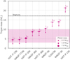 |
Fig. 8 Upper limits on the masses of trojan bodies located at the exact Lagrangian points of the nine systems studied. The symbol size scales as the mass of the planet. The mass of Neptune is denoted for reference and the shaded region represents the super-Earth mass regime. |
5 Discussion and conclusions
We have used information from the radial velocity, transit, and TTVs techniques to constrain the presence of co-orbital bodies in nine planetary systems previously showing hints of their presence (Lillo-Box et al. 2018a). These systems correspond to short-period (P < 5 days) mainly massive planets, where high-precision measurements from the three techniques can be obtained and found in the archive. The three techniques complement each other in the parameter space composed by the trojan mass vs. libration amplitude, allowing us to progressively discard trojans at different regimes.
For instance, in Fig. 8, we show the upper mass limits for co-orbitals exactly at the Lagrangian points of eight of the studied systems combining all three techniques. As we can see, we can discard trojans more massive than 10 M⊕ in six of the systems and we can go down to 5 M⊕ regime in the case of HAT-P-23, WASP-77A, and HAT-P-20. The key observations in these three systems have been the combination of more than three transit observations of the Lagrangian passage with photometric precisions at the ~1 mmag level with CAFOS and WiFSIP. In the case of WASP-5, the key technique was the radial velocity follow up with HARPS combined with the accurate measurements of the planet’s mid-transit time and mid secondary eclipse time (breaking the degeneracy with the eccentricity).
We show that ground-based photometric exploration of the Lagrangian points of known planets can provide constraints on trojan bodies in these regions down to the Earth-size regime when combining > 3 epochs with mmag precision for solar-like stars. It is important to note that intensive ground-based monitoring from small robotic telescopes would strongly increase the sample of explored systems in an efficient way.
The exploration of Kepler/K2 data was partly carried out by Janson (2013) with no positive detections. However, Hippke & Angerhausen (2015) found clear dimming at L4 and L5 of the combined Kepler light curve obtained by stacking all planet candidates, showing that on average all Kepler planets have co-orbitals of few hundreds of kilometers size (or equivalently swarms of small trojans with an equivalent cross-section of this size). Hence, a dedicated exploration of this data (taking into account possible large libration amplitudes) should reveal the presence of the individual co-orbitals (Lillo-Box et al., in prep.). In the future, TESS photometry (Ricker et al. 2014) will also help to find these bodies in many systems with precisions similar to Kepler and a 2 min cadence for many of them, which is critical in case of large libration amplitudes. Additionally, the CHEOPS mission (Broeg et al. 2013) will be a unique opportunity to follow up on the best candidates, reaching lower trojan radii down to the rocky regime.
Acknowledgements
We thank the referee for her/his useful comments during this process. We also thank Mathias Zechmeister for his useful advise and support with the SERVAL pipeline for CARMENES, which is partly used in our new pipeline to obtain the radial velocities with the CCF technique (carmeneX); and Hervé Bouy for setting and handling of the DANCE computer cluster used to analyze the data. J.L.-B. acknowledges financial support from the European Southern Observatory (ESO). Parts of this work have been carried out within the frame of the National Centre for Competence in Research PlanetS supported by the SNSF. D.B. acknowledges financial support from the Spanish grant ESP2015-65712-C5-1-R. N.C.S., P.F., and J.F. were supported by Fundação para a Ciência e a Tecnologia (FCT, Portugal) through the research grant through national funds and by FEDER through COMPETE2020 by grant PTDC/FIS-AST/1526/2014 & POCI-01-0145-FEDER-016886, as well as through Investigador FCT contracts nr. IF/01037/2013CP1191/CT0001 and IF/00169/2012/CP0150/CT0002. J.J.N. also acknowledges support from FCT though the PhD: Space fellowship PD/BD/52700/2014. A.C. acknowledges support from CIDMA strategic project (UID/MAT/04106/2013), ENGAGE SKA (POCI-01-0145-FEDER-022217), and PHOBOS (POCI-01-0145-FEDER-029932), funded by COMPETE 2020 and FCT, Portugal. H.P. has received support from the Leverhulme Research Project grant RPG-2012-661.
Appendix A Figures
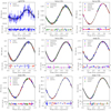 |
Fig. A.1 Radial velocity analysis of the nine studied systems. The colors of the symbols represent the instrument used; HARPSN isHARPS-N data from the archive, and HARPSNX and HARPSX are newly acquired data with HARPS-N and HARPS(respectively) in the context of TROY project. All CARMENES data were also obtained for this project. |
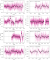 |
Fig. A.2 Light curves of all Lagrangian point transits observed with ground-based facilities. A linear baseline model accounting for time, seeing, airmass, XY positions on the detector, and background has been removed. Purple data points are the individual measurements while big black open symbols represent 10 min bins. The system and observing date (in YYMMDD format) are shown in each panel. The vertical dashed line indicates the mid-transit passage of the Lagrangian point and the dotted vertical lines indicate the total duration of the transit assuming the same as the planet. |
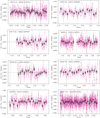 |
Fig. A.2 continued. |
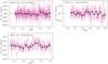 |
Fig. A.2 continued. |
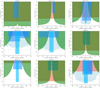 |
Fig. A.3 Constraint of the trojan mass vs. libration amplitude parameter space based on the three techniques used in this paper. The constraint from individual transits is shown as blue shaded regions with open circles, the constraint from the combined light curve is shown in light blue with open star symbols, the constraint from TTVs is shown as green diagonally striped shaded region, and the radial velocity constraint is shown as a red vertically striped shaded region. The two horizontal dotted lines represent the Earth and Neptune and are shown to guide the eye. |
Appendix B Tables
New radial velocities obtained for GJ 3470.
New radial velocities obtained for HAT-P-12.
New radial velocities obtained for HAT-P-20.
New radial velocities obtained for HAT-P-36.
New radial velocities obtained for WASP-5.
New radial velocities obtained for WASP-77 A.
New radial velocities obtained for WASP-36.
Summary of photometric data obtained for the 10 systems analyzed in this paper.
Constraints for the transit time (phase in the case of the combined transits) and depth from the individual fitting to each epoch assuming no transit is found and a linear baseline model.
References
- Aceituno, J., Sánchez, S. F., Grupp, F., et al. 2013, A&A, 552, A31 [NASA ADS] [CrossRef] [EDP Sciences] [Google Scholar]
- Appenzeller, I., & Rupprecht, G. 1992, The Messenger, 67, 18 [NASA ADS] [Google Scholar]
- Astropy Collaboration (Robitaille, T. P., et al.) 2013, A&A, 558, A33 [NASA ADS] [CrossRef] [EDP Sciences] [Google Scholar]
- Awiphan, S., Kerins, E., Pichadee, S., et al. 2016, MNRAS, 463, 2574 [NASA ADS] [CrossRef] [Google Scholar]
- Bakos, G. Á., Hartman, J., Torres, G., et al. 2011, ApJ, 742, 116 [NASA ADS] [CrossRef] [Google Scholar]
- Bakos, G. Á., Hartman, J. D., Torres, G., et al. 2012, AJ, 144, 19 [NASA ADS] [CrossRef] [Google Scholar]
- Baranne, A., Queloz, D., Mayor, M., et al. 1996, A&AS, 119, 373 [NASA ADS] [CrossRef] [EDP Sciences] [Google Scholar]
- Bastürk, O., Hinse, T. C., Özavcainodot, et al. 2015, in Living Together: Planets, Host Stars and Binaries, eds., S. M. Rucinski, G. Torres, & M. Zejda, ASP Conf. Ser., 496, 370 [NASA ADS] [Google Scholar]
- Beaugé, C., Sándor, Z., Érdi, B., & Süli, Á. 2007, A&A, 463, 359 [NASA ADS] [CrossRef] [EDP Sciences] [Google Scholar]
- Bertin, E., & Arnouts, S. 1996, A&AS, 117, 393 [NASA ADS] [CrossRef] [EDP Sciences] [Google Scholar]
- Bonfils, X., Gillon, M., Udry, S., et al. 2012, A&A, 546, A27 [NASA ADS] [CrossRef] [EDP Sciences] [Google Scholar]
- Borisov, G., Christou, A., Bagnulo, S., et al. 2017, MNRAS, 466, 489 [NASA ADS] [CrossRef] [Google Scholar]
- Bradley, L., Sipocz, B., Robitaille, T., et al. 2017, astropy/photutils: v0.4 DOI: 10.5281/zenodo.1039309 [Google Scholar]
- Broeg, C., Fortier, A., Ehrenreich, D., et al. 2013, EPJ Web Conf., 47, 3005 [Google Scholar]
- Caballero, J. A., Guàrdia, J., López del Fresno, M., et al. 2016, in Observatory Operations: Strategies, Processes, and Systems VI, Proc. SPIE, 9910, 99100E [Google Scholar]
- Charbonneau, D., Winn, J. N., Everett, M. E., et al. 2007, ApJ, 658, 1322 [NASA ADS] [CrossRef] [Google Scholar]
- Chen, J., & Kipping, D. 2017, ApJ, 834, 17 [Google Scholar]
- Collier Cameron, A., Bouchy, F., Hébrard, G., et al. 2007, MNRAS, 375, 951 [NASA ADS] [CrossRef] [Google Scholar]
- Cosentino, R., Lovis, C., Pepe, F., et al. 2012, SPIE Conf. Ser., 8446, 1 [Google Scholar]
- Faria, J. P., Haywood, R. D., Brewer, B. J., et al. 2016, A&A, 588, A31 [NASA ADS] [CrossRef] [EDP Sciences] [Google Scholar]
- Ford, E. B., & Gaudi, B. S. 2006, ApJ, 652, L137 [NASA ADS] [CrossRef] [Google Scholar]
- Ford, E. B., & Holman, M. J. 2007, ApJ, 664, L51 [NASA ADS] [CrossRef] [Google Scholar]
- Foreman-Mackey, D., Hogg, D. W., Lang, D., & Goodman, J. 2013, PASP, 125, 306 [CrossRef] [Google Scholar]
- Fuente, A., Baruteau, C., Neri, R., et al. 2017, ApJ, 846, L3 [NASA ADS] [CrossRef] [Google Scholar]
- Granata, V., Nascimbeni, V., Piotto, G., et al. 2014, Astron. Nachr., 335, 797 [NASA ADS] [CrossRef] [Google Scholar]
- Hartman, J. D., Bakos, G. Á., Torres, G., et al. 2009, ApJ, 706, 785 [NASA ADS] [CrossRef] [Google Scholar]
- Hippke, M., & Angerhausen, D. 2015, ApJ, 811, 1 [Google Scholar]
- Hoyer, S., Rojo, P., & López-Morales, M. 2012, ApJ, 748, 22 [NASA ADS] [CrossRef] [Google Scholar]
- Hoyer, S., Hamman, J., Fitzgerald, C., et al. 2017, pydata/xarray: v0.10.0 DOI: 10.5281/zenodo.1063607 [Google Scholar]
- Hrudková, M., Skillen, I., Benn, C., et al. 2009, in Transiting Planets, eds., F. Pont, D. Sasselov, & M. J. Holman, IAU Symp., 253, 446 [NASA ADS] [Google Scholar]
- Janson M. 2013, ApJ, 774, 156 [NASA ADS] [CrossRef] [Google Scholar]
- Kreidberg, L. 2015, PASP, 127, 1161 [NASA ADS] [CrossRef] [Google Scholar]
- Laughlin, G., & Chambers, J. E. 2002, AJ, 124, 592 [NASA ADS] [CrossRef] [Google Scholar]
- Laughlin, G., Chambers, J., & Fischer, D. 2002, ApJ, 579, 455 [NASA ADS] [CrossRef] [Google Scholar]
- Lee, J. W., Youn, J.-H., Kim, S.-L., Lee, C.-U., & Hinse, T. C. 2012, AJ, 143, 95 [NASA ADS] [CrossRef] [Google Scholar]
- Leleu, A., Robutel, P., & Correia, A. C. M. 2015, A&A, 581, A128 [NASA ADS] [CrossRef] [EDP Sciences] [Google Scholar]
- Leleu, A., Robutel, P., Correia, A. C. M., & Lillo-Box, J. 2017, A&A, 599, L7 [Google Scholar]
- Levison, H., Olkin, C., Noll, K., & Marchi, S. 2017, European Planetary Science Congress, 11, EPSC2017 [Google Scholar]
- Lillo-Box, J., Barrado, D., Santos, N. C., et al. 2015, A&A, 577, A105 [NASA ADS] [CrossRef] [EDP Sciences] [Google Scholar]
- Lillo-Box, J., Barrado, D., Figueira, P., et al. 2018a, A&A, 609, A96 [NASA ADS] [CrossRef] [EDP Sciences] [Google Scholar]
- Lillo-Box, J., Kipping, D., Rebollido, I., et al. 2018b, ArXiv e-prints [arXiv:1803.04010] [Google Scholar]
- Madhusudhan, N., & Winn, J. N. 2009, ApJ, 693, 784 [NASA ADS] [CrossRef] [Google Scholar]
- Mallonn, M., Nascimbeni, V., Weingrill, J., et al. 2015, A&A, 583, A138 [NASA ADS] [CrossRef] [EDP Sciences] [Google Scholar]
- Mallonn, M., Bernt, I., Herrero, E., et al. 2016, MNRAS, 463, 604 [NASA ADS] [CrossRef] [Google Scholar]
- Mancini, L., Lillo-Box, J., Southworth, J., et al. 2016, A&A, 590, A112 [NASA ADS] [CrossRef] [EDP Sciences] [Google Scholar]
- Maxted, P. F. L., Anderson, D. R., Collier Cameron, A., et al. 2013, PASP, 125, 48 [NASA ADS] [CrossRef] [Google Scholar]
- Mayor, M., Pepe, F., Queloz, D., et al. 2003, The Messenger, 114, 20 [NASA ADS] [Google Scholar]
- Meisenheimer, K. 1994, Sterne und Weltraum, 33, 516 [Google Scholar]
- Morbidelli, A., Levison, H. F., Tsiganis, K., & Gomes, R. 2005, Nature, 435, 462 [NASA ADS] [CrossRef] [PubMed] [Google Scholar]
- Murray, C. D. & Correia, A. C. M. 2010, Keplerian Orbits and Dynamics of Exoplanets, ed., S. Seager, (Tucson, AZ: University of Arizona Press), 15 [Google Scholar]
- Namouni, F., & Morais, H. 2017, Comp. Appl. Math., DOI: 10.1007/s40314-017-0489-y [Google Scholar]
- Pepe, F., Mayor, M., Galland, F., et al. 2002, A&A, 388, 632 [NASA ADS] [CrossRef] [EDP Sciences] [Google Scholar]
- Perrakis, K., Ntzoufras, I., & Tsionas, E. G. 2014, Comput. Stat. Data. Anal., 77, 54 [Google Scholar]
- Poddaný, S., Brát, L., & Pejcha, O. 2010, New Astron., 15, 297 [NASA ADS] [CrossRef] [Google Scholar]
- Quirrenbach, A., Amado, P. J., Caballero, J. A., et al. 2014, SPIE Conf. Ser., 9147, 1 [Google Scholar]
- Ricker, G. R., Winn, J. N., Vanderspek, R., et al. 2014, SPIE Conf. Ser., 9143, 20 [Google Scholar]
- Rodríguez, A., Giuppone, C. A., & Michtchenko, T. A. 2013, Celest. Mech. Dyn. Astron., 117, 59 [NASA ADS] [CrossRef] [Google Scholar]
- Schwarz, R., Bazsó, Á., Funk, B., & Zechner, R. 2015, MNRAS, 453, 2308 [NASA ADS] [CrossRef] [Google Scholar]
- Seabold, S., & Perktold, J. 2010, in Statsmodels: Econometric and Statistical Modeling with Python, 9th Python, 57 [Google Scholar]
- Smith, A. M. S., Anderson, D. R., Collier Cameron, A., et al. 2012, AJ, 143, 81 [NASA ADS] [CrossRef] [Google Scholar]
- Southworth, J., Mancini, L., Novati, S. C., et al. 2010, MNRAS, 408, 1680 [NASA ADS] [CrossRef] [Google Scholar]
- Strassmeier, K. G., Granzer, T., Weber, M., et al. 2010, Adv. Astron., 2010, 970306 [Google Scholar]
- Sun, L., Gu, S., Wang, X., et al. 2017, AJ, 153, 28 [NASA ADS] [CrossRef] [Google Scholar]
- van der Walt, S., Colbert, S. C., & Varoquaux, G. 2011, Comput. Sci. Eng., 13, 22 [CrossRef] [Google Scholar]
- Zechmeister, M., Reiners, A., Amado, P. J., et al. 2018, A&A, 609, A12 [CrossRef] [Google Scholar]
Publicly available at www.github.com/mzechmeister/serval.
Program ID: ESO 098.C-0440(A), PI: J. Lillo-Box.
Program ID: ESO 297.C-5051, PI: J. Lillo-Box.
Program ID: 18-TNG4/16A, PI: D. Barrado.
Program ID: CAHA F17-3.5-007, PI: Lillo-Box.
Program ID: CAHA H17-3.5-024, PI: Lillo-Box.
Program IDs: H17-2.2-018 and F18-2.2-004, PI: J. Lillo-Box.
The pipeline is written in Python and built on top of Astropy (Astropy Collaboration 2013), Photutils (Bradley et al. 2017), xarray (Hoyer et al. 2017), StatsModels (Seabold & Perktold 2010), NumPy (van der Walt et al. 2011), and SciPy.
Program IDs: 52-Stella9/17B and 49-Stella4-18A, PI: D. Barrado.
Program ID: ESO 298.C-5009, PI: J. Lillo-Box.
We note that at the VLT, this can be carried out via bad-AO. However, this can introduce additional systematics in the relative photometry.
See http://dan.iel.fm/emcee for further documentation.
https://github.com/exord/bayev. This code is a python implementation by R. Díaz of the formalism explained in Perrakis et al. (2014).
We note that ζ = λp − λt is the angular difference between the mean longitude of the planet (λp) and the mean longitude of the trojan (λt).
The estimated eclipse depth for this planet is smaller than 25 ppm. This is at the limit precision that will be achievable by the James Webb Space Telescope.
All Tables
Summary of the data used in this paper for the nine targets analyzed, including the number of data points for each technique, both new (Nnew) and from archive data (Narch).
Summary of photometric data obtained for the 10 systems analyzed in this paper.
Constraints for the transit time (phase in the case of the combined transits) and depth from the individual fitting to each epoch assuming no transit is found and a linear baseline model.
All Figures
|
Fig. 1 Comparison between the α values obtained with the new data (circles) and the values published in Lillo-Box et al. (2018a). The colored dotted lines represent the 3σ uncertainties. The blue colors indicate α ± σ > 0 (i.e., candidate) and red colors indicate α − σ < 0 < α + σ (i.e., no detection). Top panel: close view of the region around α = 0 |
| In the text | |
|
Fig. 2 Example of the light curve analysis of the L5 region of HAT-P-36 b (observed with CAFOS on 2018-03-22) including the linear baseline model (see Sect. 3.2.1). Top panel: raw light curve (violet symbols) together with the 15 min binned data (black open circles, for visualization purposes) and the baseline model fitted. In this case, we assume to trojan (null hypothesis). Bottom panel: baseline-corrected light curve with the detectable limit calculated as the 95% interval for the Rt ∕R⋆ parameter in the trojan model. In both panels, the shaded regions correspond to the 68.7% and 99.7% confidence intervals. |
| In the text | |
|
Fig. 3 Example of the analysis of the parameter space constrain based on the non-detection of transits in our data for the system WASP-77A. Top panel: orbit number (X-axis) vs. the orbital phase covered by our observations (red vertical lines). The transit of the Lagrangian point (L5 in this case) is expected to happen between the dotted horizontal lines. The colored lines represent a small sample of the accepted models. For a model to be accepted it has to either not cross the red lines if the trial trojan radius is larger than the light curve detectability limit (blue lines) or if the trojan transits during our observations but is smaller than the detectability limit (green lines). The bottom panels are just close views on each of the four epochs, where the X-axis is the phase from the Lagrangian point conjunction. |
| In the text | |
|
Fig. 4 Example of the light curve combination in phase for the case of WASP-77A. The individual epochs are shown in the top panel (after removing the linear baseline model) and the combined light curve is shown in the bottom panel; 10 min bins have 225 ppm rms. The vertical dotted lines indicate the expected transit ingress and egress of the Lagrangian point. |
| In the text | |
|
Fig. 5 Detailed example of the constraining of the trojan mass vs. libration amplitude parameter space in the case of WASP-77A.Negative (positive) values for the libration amplitude are used to represent constraints on transits before (after) the Lagrangian point passage. Only the white region is not explored by our data. |
| In the text | |
|
Fig. 6 Trojan hypothesis model after removing the linear baseline model for HAT-P-20. This trojan model is only favored against the null hypothesis if we include the whole data set. However by removing the feature at phases ϕ > 0.20, the null hypothesis is favored. The black shaded vertical line represents the expected egress of the Lagrangian point, showing thelarge time lag of the would-be trojan transit. This light curve corresponds to the data from CAFOS at CAHA on 2017-12-09. |
| In the text | |
|
Fig. 7 Parameter space of trojan’s eccentricity vs. libration amplitude constrained by the non-detection of transits in the four Lagrangian passages observed for WASP-77A b. The results show that only highly eccentric orbits are possible for any libration amplitude and that low eccentric orbits are still allowed for libration amplitudes larger than 35°. |
| In the text | |
|
Fig. 8 Upper limits on the masses of trojan bodies located at the exact Lagrangian points of the nine systems studied. The symbol size scales as the mass of the planet. The mass of Neptune is denoted for reference and the shaded region represents the super-Earth mass regime. |
| In the text | |
|
Fig. A.1 Radial velocity analysis of the nine studied systems. The colors of the symbols represent the instrument used; HARPSN isHARPS-N data from the archive, and HARPSNX and HARPSX are newly acquired data with HARPS-N and HARPS(respectively) in the context of TROY project. All CARMENES data were also obtained for this project. |
| In the text | |
|
Fig. A.2 Light curves of all Lagrangian point transits observed with ground-based facilities. A linear baseline model accounting for time, seeing, airmass, XY positions on the detector, and background has been removed. Purple data points are the individual measurements while big black open symbols represent 10 min bins. The system and observing date (in YYMMDD format) are shown in each panel. The vertical dashed line indicates the mid-transit passage of the Lagrangian point and the dotted vertical lines indicate the total duration of the transit assuming the same as the planet. |
| In the text | |
|
Fig. A.2 continued. |
| In the text | |
|
Fig. A.2 continued. |
| In the text | |
|
Fig. A.3 Constraint of the trojan mass vs. libration amplitude parameter space based on the three techniques used in this paper. The constraint from individual transits is shown as blue shaded regions with open circles, the constraint from the combined light curve is shown in light blue with open star symbols, the constraint from TTVs is shown as green diagonally striped shaded region, and the radial velocity constraint is shown as a red vertically striped shaded region. The two horizontal dotted lines represent the Earth and Neptune and are shown to guide the eye. |
| In the text | |
Current usage metrics show cumulative count of Article Views (full-text article views including HTML views, PDF and ePub downloads, according to the available data) and Abstracts Views on Vision4Press platform.
Data correspond to usage on the plateform after 2015. The current usage metrics is available 48-96 hours after online publication and is updated daily on week days.
Initial download of the metrics may take a while.