| Issue |
A&A
Volume 618, October 2018
|
|
|---|---|---|
| Article Number | A125 | |
| Number of page(s) | 30 | |
| Section | Stellar structure and evolution | |
| DOI | https://doi.org/10.1051/0004-6361/201832977 | |
| Published online | 23 October 2018 | |
GRAVITY chromatic imaging of η Car’s core
Milliarcsecond resolution imaging of the wind-wind collision zone (Brγ, He I)
1 Max Planck Institute for Astronomy, Königstuhl 17, 69117 Heidelberg, Germany
e-mail: This email address is being protected from spambots. You need JavaScript enabled to view it.
2 LESIA, Observatoire de Paris, PSL Research University, CNRS, Sorbonne Universités, UPMC Univ. Paris 06, Univ. Paris Diderot, Sorbonne Paris Cité, France
3 Univ. Grenoble Alpes, CNRS, IPAG, 38000 Grenoble, France
4 I. Physikalisches Institut, Universität zu Köln, Zülpicher Str. 77, 50937 Köln, Germany
5 Universidade do Porto – Faculdade de Engenharia, Rua Dr. Roberto Frias, 4200-465 Porto, Portugal
6 CENTRA, Instituto Superior Tecnico, Av. Rovisco Pais, 1049-001 Lisboa, Portugal
7 European Southern Observatory, Karl-Schwarzschild-Str. 2, 85748 Garching, Germany
8 European Southern Observatory, Casilla, 19001 Santiago 19, Chile
9 Max Planck Institute for Extraterrestrial Physics, Giessenbachstrasse, 85741 Garching bei München, Germany
10 Dublin Institute for Advanced Studies, 31 Fitzwilliam Place, D02 XF86 Dublin, Ireland
11 Max-Planck-Institute for Radio Astronomy, Auf dem Hügel 69, 53121 Bonn, Germany
12 Department of Physics, Le Conte Hall, University of California, Berkeley, CA, 94720 USA
13 Unidad Mixta Internacional Franco-Chilena de Astronomía (CNRS UMI 3386), Departamento de Astronomía, Universidad de Chile, Camino El Observatorio 1515, Las Condes, Santiago, Chile
14 Sterrewacht Leiden, Leiden University, Postbus 9513, 2300 RA Leiden, The Netherlands
15 Department of Physics and Astronomy, University of Sheffield, Hicks Building, Hounsfield Rd., Sheffield, S3 7RH UK
16 Observatoire de Genève, Université de Genève, 51 Ch. des Maillettes, 1290 Sauverny, Switzerland
17 ONERA, The French Aerospace Lab, Châtillon, France
18 European Space Agency, Space Telescope Science Institute, Baltimore, USA
19 Faculdade de Ciências, Universidade de Lisboa, Edifício C8, Campo Grande, 1749-016 Lisbon, Portugal
20 School of Physics, Astrophysics Group, University of Exeter, Stocker Road, Exeter, EX4 4QL UK
Received:
7
March
2018
Accepted:
16
July
2018
Abstract
Context. η Car is one of the most intriguing luminous blue variables in the Galaxy. Observations and models of the X-ray, ultraviolet, optical, and infrared emission suggest a central binary in a highly eccentric orbit with a 5.54 yr period residing in its core. 2D and 3D radiative transfer and hydrodynamic simulations predict a primary with a dense and slow stellar wind that interacts with the faster and lower density wind of the secondary. The wind-wind collision scenario suggests that the secondary’s wind penetrates the primary’s wind creating a low-density cavity in it, with dense walls where the two winds interact. However, the morphology of the cavity and its physical properties are not yet fully constrained.
Aims. We aim to trace the inner ∼5–50 au structure of η Car’s wind-wind interaction, as seen through Brγ and, for the first time, through the He I 2s-2p line.
Methods. We have used spectro-interferometric observations with the K-band beam-combiner GRAVITY at the VLTI. The analyses of the data include (i) parametrical model-fitting to the interferometric observables, (ii) a CMFGEN model of the source’s spectrum, and (iii) interferometric image reconstruction.
Results. Our geometrical modeling of the continuum data allows us to estimate its FWHM angular size close to 2 mas and an elongation ratio ϵ = 1.06 ± 0.05 over a PA = 130° ± 20°. Our CMFGEN modeling of the spectrum helped us to confirm that the role of the secondary should be taken into account to properly reproduce the observed Brγ and He I lines. Chromatic images across the Brγ line reveal a southeast arc-like feature, possibly associated to the hot post-shocked winds flowing along the cavity wall. The images of the He I 2s-2p line served to constrain the 20 mas (∼50 au) structure of the line-emitting region. The observed morphology of He I suggests that the secondary is responsible for the ionized material that produces the line profile. Both the Brγ and the He I 2s-2p maps are consistent with previous hydrodynamical models of the colliding wind scenario. Future dedicated simulations together with an extensive interferometric campaign are necessary to refine our constraints on the wind and stellar parameters of the binary, which finally will help us predict the evolutionary path of η Car.
Key words: instrumentation: interferometers / instrumentation: high angular resolution / stars: mass-loss / stars: massive / stars: imaging / binaries: general
GRAVITY is developed in a collaboration by the Max Planck Institute for Extraterrestrial Physics, LESIA of Paris Observatory and IPAG of Université Grenoble Alpes/CNRS, the Max Planck Institute forAstronomy, the University of Cologne, the Centro Multidisciplinar de Astrofisica Lisbon and Porto, and the European Southern Observatory.
© ESO 2018
1. Introduction
Massive stars are among the most important chemical factories of the interstellar medium (ISM). This is mainly because their evolution and fate are highly affected by strong stellar winds (vw ∼ 103 km s−1),high mass-loss rates (Ṁ ∼ 10−5 –10−3M⊙ yr−1) and deaths as supernovae (SNe; see, e.g., Conti & Niemelä 1976; Langer et al. 1994; Meynet & Maeder 2003; Meynet et al. 2011). One of the evolutionary stages of high-mass stars that exhibit sporadic but violent mass-loss episodes is the luminous blue variable (LBV) phase (Humphreys & Davidson 1994). The importance of LBVs to stellar evolution models relies on the possibility of them to directly explode as SN without being a Wolf-Rayet (WR) star (Smith 2007; Smith et al. 2011; Trundle et al. 2008). Therefore, detailed studies of LBVs are crucial to understand the mass-loss processes in high-mass stars (see e.g., Pastorello et al. 2010; Smith et al. 2011).
The source, η Car, is one of the most intriguing LBVs in the Galaxy. Located at the core of the Homunculus Nebula in the Trumpler 16 cluster at a distance of 2.3 ± 0.1 kpc (Walborn 1973; Allen & Hillier 1993; Smith 2006), it has been identified as a luminous (Ltot ≥ 5 × 10⁶L⊙Davidson & Humphreys 1997; Smith et al. 2003) colliding-wind binary (Damineli et al. 1997, Damineli et al. 2008a,b; Hillier et al. 2001; Corcoran et al. 2010) in a highly eccentric orbit (e ∼ 0.9; Corcoran 2005) with a period of 2022.7 ± 1.3 d (Damineli et al. 2008a).
The primary, ηA, is a very massive star with an estimated M∼ 100 M⊙, a mass-loss rate Ṁ ∼ 8.5 × 10⁻⁴ M⊙ yr−1 and a wind terminal speed v∞ ∼ 420 km s−1 (Hillier et al. 2001, 2006; Groh et al. 2012a,b). Evidence suggests that ηA is near the Eddington limit (Conti 1984; Humphreys & Davidson 1994). Therefore, it loses substantial mass in violent episodes such as the “Great Eruption” where ∼15 M⊙, possibly more than 40 M⊙ (Gomez et al. 2010; Morris et al. 2017), were ejected over a period of ∼10 yr. Mass-loss events dominate the evolutionary tracks of the most massive stars (Langer 1998; Smith 2006). In binary star systems, like η Car, the presence of a companion affects wind-driven mass loss, providing alternative evolutionary pathways compared to single stars. Therefore, understanding in detail their mass-loss processes is particularly important.
The nature of the secondary, ηB, is even less constrained since it has not been directly observed (it is, at least, of the order of 100 times fainter than ηA;Weigelt et al. 2007) because it is embedded in the dense wind of the primary. Models of the X-ray emission (kT ∼ 4 − 5 keV) predict a wind terminal velocity v∞ ∼ 3000 km s−1, a mass-loss rate Ṁ ∼ 10−5 M⊙ yr−1 (Pittard & Corcoran 2002; Okazaki et al. 2008; Parkin et al. 2011), and a Teff ∼ 36 000 − 41 000 K (Teodoro et al. 2008).
Models of the mutual motion of the stars suggest an inclination i∼ 130–145°, an argument of periastron ω∼ 240–285°, and a sky projected PA ∼ 302 − 327° for the best-fit orbital solution (Damineli et al. 1997; Okazaki et al. 2008; Parkin et al. 2009, 2011; Groh et al. 2010b; Gull et al. 2011; Madura & Groh 2012; Madura et al. 2012; Teodoro et al. 2016). This suggests that the orbital plane of the binary is almost perpendicular to the Homunculus axis (i∼ 49° with respect to the sky plane; PA ∼ 132°;Davidson et al. 2001; Smith 2006). These orbital parameters also imply that the secondary remains in front of the primary (in the line-of-sight -LOS- of the observer) most of the time during the orbital motion, except close to the periastron, where ηB goes behind ηA and it is obscured by the dense primary wind.
Figure 1 displays the inclination and PA of the Homunculus Nebula and of the orbit of ηB around ηA, according to the orbital solution reported by Teodoro et al. (2016). The left panel displays the nebula projected in the plane of the sky. The PA (east to the north) of the semi-major axis is labeled in the image. The right panel displays the position of the nebula and of the orbit of the binary in a plane parallel to the observer’s line-of-sight and the sky plane. The inclination angles (relative to the sky plane) of the nebula (iHN) and of the binary’s orbital plane (iBinary) are labeled.
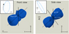 |
Fig. 1. Homunculus Nebula and the binary orbit projected in the plane of the sky (left panel; front view) and in a plane formed by the observer’s LOS and the sky plane (right panel; side view). The 3D Homunculus model was obtained from the online resources of Steffen et al. (2014). |
The secondary, ηB, photoionizes part of the primary wind, changing the strength of lines such as Hα, He I, [Fe II], and [Ne II] (Hillier et al. 2001; Nielsen et al. 2007; Mehner et al. 2010, 2012; Madura et al. 2012; Davidson et al. 2015). Additionally, it ionizes the inner 1″ circumstellar ejecta (Weigelt & Ebersberger 1986; Hofmann & Weigelt 1988; Weigelt et al. 1995). 2D radiative transfer models and 3D hydrodynamical simulations of the wind-wind collision scenario suggest that the high-velocity secondary wind penetrates the slower and denser primary wind creating a low-density cavity in it, with thin and dense walls where the two winds interact (Okazaki et al. 2008; Groh et al. 2012a; Madura et al. 2012; Madura et al. 2013; Clementel et al. 2015a,b). This wind-wind collision scenario produces the shock-heated gas responsible for the X-ray variability, and the ionization effects observed in the optical, infrared, and ultraviolet spectra.
These aforementioned models also show that during the periastron passage (phase ϕ∼ 0.98–1.02) the acceleration zone of the post-shock wind of ηB is affected by ηA. The hot wind of ηB pushes the primary wind outward and it ends up trapped inside the cavity walls. The material in the walls is accelerated to velocities larger than ηA’s wind terminal velocity, creating a layer of dense trapped primary wind. These layers have been observed as concentric fossil wind arcs in [Fe II] and [Ni II] images at the inner 1″ obtained with the HST/STIS camera (Teodoro et al. 2013; Gull et al. 2016).
To explain the wind-wind phenomenology at 2–10 mas (∼5–25 au) scales, several attempts have been made to characterize the core of η Car. Particularly, long-baseline infrared interferometry has been a decisive technique for such studies. Kervella et al. (2002) and van Boekel et al. (2003) resolved an elongated optically thick region using the K-band (2.0–2.4 μm) beam-combiner VINCI (Kervella et al. 2000) at the Very Large Telescope Interferometer (VLTI; Glindemann et al. 2003). Those authors measured a size of 5–7 mas (11–15 au) for η Car’s core, with a major to minor axis ratio ϵ = 1.25 ± 0.05, and a PA = 134 ± 7°. Using a non-local thermal equilibrium (non-LTE) model, a mass-loss rate of 1.6 ± 0.3 × 10⁻³ M⊙ yr−1 was estimated.
Follow-up observations (Weigelt et al. 2007) with the K-band beam combiner VLTI-AMBER (Petrov et al. 2007) using medium (R = 1500) and high (R = 12 000) spectral resolutions of the He I 2s-2p (2.0587 μm) and Brγ (2.1661 μm) lines, resolved η Car’s wind structure at angular scales as small as ∼6 mas (∼13 au). These authors measured a (50% encircled energy) diameter of 3.74–4.23 mas (8.6–9.7 au) for the continuum at 2.04 μm and 2.17 μm; a diameter of 9.6 mas (22.6 au) at the peak of the Brγ line; and 6.5 mas (15.3 au) at the emission peak of the He I 2s-2p line. They also confirmed the presence of an elongated optically thick continuum core with a measured axis ratio ϵ = 1.18 ± 0.10 and a projected PA = 120° ± 15°.
The observed non-zero differential phases and closure phases indicate a complex extended structure across the emission lines. To explain the Brγ-line profile and the signatures observed in the differential and closure phases, Weigelt et al. (2007) developed a “rugby-ball” model for an optically thick, latitude dependent wind, which includes three components: (a) a continuum spherical component; (b) a spherical primary wind; (c) and a surrounding aspherical wind component inclined 41° from the observer’s LOS.
New high-resolution AMBER observations in 2014 allowed Weigelt et al. (2016) to reconstruct the first aperture-synthesis images across the Brγ line. These images revealed an asymmetric and elongated structure, particularly in the blue wing of the line. At velocities between −140 and −380 km s−, the intensity distribution of the reconstructed maps shows a fan-shaped structure with an 8.0 mas (18.8 au) extension to the southeast and 5.8 mas (13.6 au) to the northwest. The symmetry axis of this elongation is at a PA = 126°, which coincides with that of the Homunculus axis. This fan-shaped morphology is consistent with the wind-wind collision cavity scenario described by Okazaki et al. (2008), Madura et al. (2012, 2013), and Teodoro et al. (2013, 2016), with the observed emission originating mainly from the material flowing along the cavity in a LOS preferential toward the southeast wall.
Additionally to the wind-wind collision cavity, several other wind structures were discovered in the images reported by Weigelt et al. (2016). At velocities between −430 and −340 km s−1, a bar-like feature appears to be located southwest of the continuum. This bar has the same PA as the more extended fossil wind structure reported by Falcke et al. (1996) and Gull et al. (2011, 2016), that may correspond to an equatorial disk and/or toroidal material that obscures the primary star in the LOS. At positive velocities, the emission appears not to be as extended as in the blue-shifted part of the line. This may be because we are looking at the back (red-shifted) part of the primary wind that is less extended because it is not as deformed by the wind collision zone. Finally, the wind lacks any strong emission line features at velocities lower than −430 km s−1 or larger than +400 km s−1.
This work presents VLTI-GRAVITY chromatic imaging of η Car’s core across two spectral lines in the infrared K-band: He I 2s-2p and Brγ. The paper is outlined as follows: Sect. 2 presents our GRAVITY observations and data reduction. In Sect. 3 the analyses of the interferometric observables, and the details of the imaging procedure are described. In Sect. 4 our results are discussed and, finally, in Sect. 5 the conclusions are presented.
2. Observations and data reduction
2.1. Observations
The milliarcsecond resolution of GRAVITY (Eisenhauer et al. 2008, 2011; Gravity Collaboration 2017) enables spectrally resolved interferometric imaging of the central wind region of η Car. At an apparent magnitude of mK = 0.94 mag, the target is bright enough for observations with the 1.8-m Auxiliary Telescopes (ATs). η Car was observed during the nights of February 24th and 27th, 2016, as part of the commissioning phase of the instrument, and during the nights of May 30th and July 1st 2017, as part of the GRAVITY Guaranteed Time Observations (GTO). The observations were carried out using the highest spectral resolution (R = 4000) of the GRAVITY beam combiner, together with the split-polarization and single-field modes of the instrument. With this configuration, GRAVITY splits the incoming light of the science target equally between the fringe tracker and science beam combiner to simultaneously produce interference fringes in both. While the science beam combiner disperses the light at the desired spectral resolution, the fringe tracker works with a low-spectral resolution of R ∼ 22 (Gillessen et al. 2010) but at a high temporal sampling (∼1 kHz). This allows to correct for the atmospheric piston, and to stabilize the fringes of the science beam combiner.
For the 2016 observations, ten data sets were recorded with the A0-G1-J2-K0 array plus four more with the A0-G2-J2-J3 configuration. The u−v coverage obtained (Fig. 2) provides a maximum projected baseline of ∼130 m (J2-A0) that corresponds to a maximum angular resolution (θ = λ/2B; where B is the maximum baseline) of θ = 1.75 mas, at a central wavelength of λ0 = 2.2 μm. The 2017 observations comprise three data sets with the D0-B2-J3-K0 array plus seven data sets with the A0-G1-J2-K0 array. For this second epoch the maximum baseline length (J2-A0) was around 122 m (θ = 1.85 mas). However, since most of the longest baselines for both imaging epochs are of 100 m, we adopted a mean maximum angular resolution θ = 2.26 mas for our imaging program. Tables A.1 and A.2 list individual data sets and observing conditions.
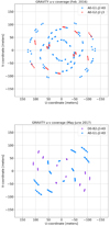 |
Fig. 2. η Car’s u−v coverages obtained during the GRAVITY runs in February 2016 (top panel) and May-June 2017 (bottom panel). Different quadruplets are indicated with different colors. |
2.2. Data reduction
The interferometric observables (squared visibilities, closure phases, and differential phases) as well as the source’s spectrum were obtained using versions 0.9.0 and 1.0.7 of the GRAVITY data reduction software1 (Lapeyrere et al. 2014). More details on the data reduction procedure are provided in Sanchez-Bermudez et al. (2017). To calibrate the interferometric observables, interleaved observations of the science target and a point-like source were performed. We used the K3 II star HD 89682 (K-band Uniform Disk diameter dUD = 2.88 mas) as interferometric calibrator for both epochs. Before analyzing the data, all the squared visibility (V2) points with a signal-to-noise ratio (S/N) ≤ 5 and closure phases with σcp ≥ 40° were excluded from the analysis.
2.3. Calibration of η Car’s integrated spectrum
For each one of the data sets, four samples of η Car’s integrated spectrum were obtained with GRAVITY. The data reduction software delivers the spectrum flattened by the instrumental transfer function obtained from the Pixel to Visibility Matrix (P2VM; Petrov et al. 2007). Additionally, GRAVITY uses the internal calibration unit (Blind et al. 2014) to obtain the fiber wavelength scale, producing a wavelength map with a precision of Δλ = 2 nm. Apart from this preliminary calibrations, we had to correct the η Car spectrum for the atmospheric transfer function together with a more precise wavelength calibration. For this purpose, we used the following method:
-
1.
A weighted average science and calibrator spectra were computed from the different samples obtained with GRAVITY.
-
2.
To refine the wavelength calibration, we used a series of telluric lines across the spectrum of our interferometric calibrator. A Gaussian was fitted to each one of the lines profiles recording their peak positions. The high-resolution (R = 40 000) telluric spectrum at the Kitt Peak observatory was then used as reference to re-calibrate the GRAVITY wavelength map. For this, we first degraded the reference spectrum to the GRAVITY resolution and then, we identified a mean wavelength shift of the calibrator’s tellurics from the Kitt Peak ones. Finally, the GRAVITY wavelength map was corrected. With this method, we reached a 1σ wavelength calibration error relative to the reference spectrum of 1.23 Å (Δv = 16.8 km s−1 at λ0 = 2.2 μm) for the 2016 data, and 0.67 Å (Δv = 9.1 km s−1) for the 2017 data, respectively. A similar calibration method was used by Weigelt et al. (2007, 2016) on the previously reported η Car AMBER data.
-
3.
Once the wavelength calibration was performed, we remove the atmospheric transfer function from the η Car spectrum by obtaining the ratio of the science target and of the interferometric calibrator spectra. Since the interferometric calibrator, HD 89682, is a K3 II star, we have to correct for its intrinsic photospheric lines (e.g., the CO bands seen in absorption from 2.29 μm onward). For this purpose, we used a theoretical BT-Settl2 model (see Allard et al. 2012) of a star with a Teff = 4200 K, a log(g)=1.5, and Z = −0.5. Figure 3 displays the normalized η Car spectrum with all the lines, between 2.0 μm and 2.2 μm, with interferometric signals different from the continuum labeled. Although the 2016 spectrum appears to be slightly noisier than the 2017 one, no significant differences were found between the two GRAVITY epochs. This work focuses on the interferometric imaging of η Car across He I 2s-2p and Brγ. Figure 4 displays the normalized η Car spectrum at these wavelengths, together with the differential visibilities and phases of one of our interferometric data sets. Notice the strong changes of the observables between the continuum and the lines.
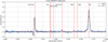
Fig. 3. 2016 (blue straight line) and 2017 (black straight line) η Car normalized spectra in the 2.0–2.2 μm bandpass. The vertical red-dashed lines indicate the spectral features identified in the spectrum.
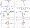
Fig. 4. Normalized GRAVITY spectrum at the position of the He I 2s-2p and Brγ lines. The calibrated differential visibilities (middle) and phases (bottom) of one of the GRAVITY data sets (MJD: 57903.9840) are also shown. In the middle and bottom panels, different colors correspond to each one of the baselines in the data set (see label on the plots). The dashed-red vertical lines indicate the reference wavelength of the emission feature, and the dashed-horizontal lines show the reference value of the continuum baseline.
2.4. Ancillary FEROS spectrum
To complement the analysis of the η Car GRAVITY spectrum, we obtained four optical high-resolution spectra of the source using the Fiber-fed Extended Range Optical Spectrograph (FEROS; Kaufer & Pasquini 1998) at the MPG 2.2 m telescope at La Silla Observatory in Chile. FEROS covers the entire optical spectral range from 3600 Å to 9200 Å and provides a spectral resolution of R = 48 000. All spectra were obtained using the object-sky mode where one of the two fibers is positioned on the target star and the other fiber is simultaneously fed with the sky background. The exposure time was 15 s and 30 s for every two spectra. The reduction and calibration of the raw data were performed using the CERES pipeline (Brahm et al. 2017). Figure F.1 displays a normalized mean spectrum of the four samples.
3. Data Analysis
3.1. Geometric model to the GRAVITY Fringe Tracker data
To obtain an angular measurement of the continuum size, a geometrical model was applied to the V
2 Fringe Tracker data. The model consists of two Gaussian disks with different angular sizes tracing the compact and extended brightness distribution of the source. The expression used to estimate the complex visibilities, V(u, v), is the following one: (1)
(1)
with (2)
(2)
where F2/F1 is the flux ratio between the two Gaussian disks, (u, v) are components of the spatial frequency sampled per each observed visibility point (u = Bx/λ and v = By/λ), and θ is the fitted full-width-at-half-maximum (FWHM) angular size for each one of the components.
Since previous studies suggest an elongation of η Car’s core along the projected PA of the Homunculus semi-major axis, we applied our geometrical model to V 2 at two orientations. To cover PAs perpendicular and parallel to the semi-major axis of the nebula, we used all the V 2 points at PA⊥ = 40° ± 20° and at PA∥ = 130° ± 20°, respectively. The model optimization was done using a dedicated Markov-Chain Monte-Carlo (MCMC) routine based on the python software pymc (Patil et al. 2010). To account for the standard deviations and correlations of the model parameters, we explore the solution space over 10 000 different models, considering the first 5000 iterations as part of the burn-in phase and accepting only one every three draws of the Monte Carlo. Initial linear distributions were assumed for all the parameters. To avoid an underestimation of the error-bars, the waist of the posterior Gaussian likelihood distribution was also marginalized for each one of the fitted parameters. Figure 5 shows the best-fit model and its uncertainties. Table 1 displays the best-fit parameters of our geometrical model and Figure B.1 shows the 2D posterior distributions of the fitted parameters.
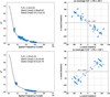 |
Fig. 5. Left panels: best-fit geometrical model to the Fringe Tracker V 2 data. The model is plotted with a black line, the data are shown with blue dots and the model parameters (with their uncertainties) are indicated on each panel. Right panels: visibility points used for each model fitting at two different position angles, PA⊥ = 40°± 20° and PA∥ = 130°± 20°. |
Best-fit parameters of the geometrical model.
3.2. Image reconstruction of the science beam combiner data
3.2.1. Chromatic reconstruction: Brγ and He I
The high accuracy of the interferometric observables allows a chromatic image reconstruction of η Car across the Brγ and He I 2s-2p lines. For this purpose, we used SQUEEZE 3 (Baron & Kloppenborg 2010), an interferometry imaging software that allows simultaneous fitting of the visibility amplitudes, squared visibilities, closure phases, and chromatic differential phases (or combinations of them). At infrared wavelengths, image reconstruction from interferometric data is constrained mainly by the (i) sparse baseline coverage and (ii) the lack of absolute phase information. Therefore, SQUEEZE applies a regularized minimization of the form: ![Mathematical equation: $ \begin{aligned} \boldsymbol{x}_{\mathrm{ML}}=\underset{\boldsymbol{x}}{\mathrm{argmin}}[1/2 \chi ^2(\boldsymbol{x})+\sum _{i}^{n}\mu _i R(\boldsymbol{x})_i]\,,\\ \end{aligned} $](/articles/aa/full_html/2018/10/aa32977-18/aa32977-18-eq3.gif) (3)
(3)
where χ2(x) is the likelihood of our data to a given imaging model, R(x)i are the (prior) regularization functions used and μi the weighting factors that trade-off between the likelihood and priors. For η Car, we used a combination of the following three different SQUEEZE regularizers:
-
1.
To avoid spurious point-like sources in the field-of-view (FOV), we applied a spatial L0-norm.
-
2.
To enhance the extended structure expected in some of the mapped spectral channels, a Laplacian was used.
-
3.
To ensure spectral continuity all over the mapped emission lines, a spectral L2-norm was applied.
For the minimization, SQUEEZE uses a Simulated Annealing Monte-Carlo algorithm as the engine for the reconstruction. We created 15 chains with 250 iterations each to find the most probable image that best-fit our interferometric data. We used a 67 × 67 pixel grid with a scale of 0.6 mas/pixel. As initial point for the reconstruction, we chose a Gaussian with a FWHM of 2 mas centered in the pixel grid, and containing 50% of the total flux. We simultaneously fitted the V2, closure phases, and wavelength-differential phases. The differential phase is defined in SQUEEZE of the following form:  (4)
(4)
where ϕ0(λi) is the measured phase at channel i, and ϕref is the reference phase. The SQUEEZE implementation of ϕ(λi) uses the REFMAP table, of the OI_VIS extension in the OIFITS v2 files (Pauls et al. 2005; Duvert et al. 2017), to determine which channels are used to define the reference phase ϕref. In our case, we defined ϕref as the average of the measured phases over the full spectral bandpass used for the reconstruction, with exception of the working channel itself, in the following way:  (5)
(5)
With this definition, the reference phase varies from channel to channel but avoids quadratic bias terms (a similar definition of ϕ(λi) has been used before to analyze AMBER data; see e.g., Millour et al. 2006, 2007; Petrov et al. 2007). While the V2 data measure the flux contribution at different spatial scales and the closure phases the asymmetry of the source, the wavelength-differential phases give information about the relative flux-centroid displacement between a given wavelength and the reference one.
For Brγ, 35 channels between 2.160 μm and 2.171 μm were imaged, while for He I, 34 channels between 2.054 μm and 2.063 μm were used. The final mean images were created through the following procedure:
-
1.
We ranked the converged chains, assigning the highest score to the one with the global χ2 closest to unity. From the ranked chains, we select the best five of them to create the final images.
-
2.
To align the selected cubes of images to a common reference pixel position, a mean centroid position of the continuum was estimated. For this purpose, the first and last five channels of each cube of images were used. The individual centroid positions were computed using a mask of five pixels around the maxima of the images at every channel used as continuum reference. Then, their mean value was computed. All the images in the cube were shifted, with sub-pixel accuracy (∼0.1 pixels), from this mean centroid position to the center of the image defined at position [34,34] in the pixel grid.
-
3.
From the aligned cubes, we compute a mean image per wavelength. Finally, since most of the spatial frequencies in the u−v coverages correspond to 100 m baselines, each image was smoothed with a 2D Gaussian with a FWHM equivalent to λ0/2Bmax = 2.26 mas.
For both lines, reconstruction tests with the s- and p-polarization data were done independently, however, no significant morphological changes were observed. The images here presented correspond to the p-polarization data. Figures 6 and 7 show the mean-reconstructed 2016 Brγ and He I images, respectively. The 2017 images are shown in Figs. D.1 and D.2. To inspect the quality of the reconstruction, Figs. E.1–E.8 display the V2 and closure phases from the recovered images together with the data.
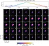 |
Fig. 6. Brγ interferometric aperture synthesis images from the Feb. 2016 data. The Doppler velocity of each frame is labeled in the images. For all the panels, east is to the left and north to the top. The displayed FOV corresponds to 36 × 36 mas. The small white ellipse shown in the lowermost-left panel corresponds to the synthesized primary beam (the detailed PSF is shown in Fig. D.1). Above all the images, the GRAVITY spectrum is shown and the different positions where the images are reconstructed across the line are labeled with a colored square, which is also plotted in the images for an easy identification. |
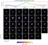 |
Fig. 7. He I interferometric aperture synthesis images from the Feb. 2016 data. The maps are as described in Fig. 6. |
3.2.2. Effects of the u − v coverage on the reconstructed images
Due to the interacting winds of the eccentric binary at the core of η Car, we expect changes in the spatial distribution of the flux at different orbital phases. This condition could explain the differences in the observed morphologies between our two imaging epochs. However, while the u−v coverage of the 2016 data is homogeneous, the 2017 u−v coverage is more sparse. The sparseness of the 2017 u−v coverage was caused, partially, because the target was observable above 35° over the horizon only for a few hours at the beginning of the night.
Therefore, the long baselines of our interferometric array could not properly sample north-south orientations of the u−v space. This sparseness in the u−v coverage produced a clumpy fine structure and a cross-like shape, superimposed on the source’s emission, on the reconstructed images. This cross-like structure is caused by the strong secondary lobes and the elongation of the primary beam (see Fig. C.1). This effect could mimic or mask real changes in the morphology associated with the physics of the wind-wind interactions with the synthesized beam and/or artifacts in the reconstruction process.
To detect the morphological changes between two epochs associated to the physical conditions of the source and not caused by the u−v coverage, we searched for coincidental baselines (in size and position angle) at both epochs, to compare the differential phases and visibilities between them. This test allows us to monitor the flux centroid evolution between the continuum and the lines together with the changes observed in the flux distribution. Three baselines, tracing the small, intermediate and large angular scales were selected. Additionally, we compute the differential observables from the reconstructed images to monitor the goodness of the images recovering the possible morphological changes.
Figure 8 displays, as an example, the results of this comparison for Brγ. For the short (θ= 5.7 mas; 13.4 au) and intermediate (θ= 3.8 mas; 8.4 au) baselines, the overall signatures of the centroid and of the flux distribution are similar at both epochs, with more prominent centroid changes at blue-shifted velocities than at the red-shifted side. The long (θ=1.9 mas; 4.46 au) baseline shows more drastic differences at blue-shifted velocities between the two epochs. For example, while the differential phases of the 2017 data exhibit an upside-down double-peak profile at velocities between −420 km s−1 and −170 km s−1, the 2016 shows a single and less prominent peak.
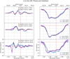 |
Fig. 8. Differential phases (left panels) and differential visibilities (right panels) between the continuum and the line emission for the 2016 (blue line) and 2017 data (purple line). The (reference) continuum phase and visibility were estimated using the first and last five channels in the imaged bandpass. Each one of the rows corresponds to a similar baseline in both epochs, tracing large (top), intermediate (middle) and small (bottom) spatial scales. The baseline lengths and position angles are labeled on the left panels, while the baseline stations are labeled on the right ones. The black-dashed lines correspond to the differential quantities extracted from the unconvolved reconstructed images. The vertical red-dotted line marks the systemic velocity of Brγ. The horizontal red-dotted lines show the continuum baselines. |
These changes in the observables for coincidental baselines provide evidence of modifications in the brightness distribution between the two epochs. However, despite the good fit of the 2017 images to the observables (see Figs. E.3, E.4, E.7, and E.8), it is clear that the sparse u−v coverage of the second epoch strongly detriments the quality of the reconstructed images. Therefore, they cannot be used for a proper (direct) comparison of the global morphology observed in the 2016 data. Thus, the 2017 images were excluded for the following analysis and discussion.
4. Discussion
4.1. Spectroscopic analysis of η Car’s primary wind
To characterize the properties of ηA’s wind, we fitted the integrated spectrum of our GRAVITY observations (Sect. 2.3) with model spectra. The synthetic spectra were computed with the 1D spherical non-LTE stellar atmosphere and radiative transfer code CMFGEN (Hillier & Miller 1998). Our atomic model includes a large number of ionization stages to cover a wide temperature range in our stellar atmosphere grid without changing the atomic model. The following ions were taken into account: H I, He I-II, C I-IV, N I-IV, O I-IV, Ne I-IV, Na I-IV, Mg I-IV, Ca I-IV, Al I-IV, Si I-IV, P II-V, S I-V, Ar I-IV, Fe I-V, and Ni II-V; and the metallicity was set to solar according to Asplund et al. (2005). For comparison, we computed a reference spectrum with the stellar parameters derived by Groh et al. (2012a) for the primary, which in turn is based on previous estimates by Hillier et al. (2001, 2006). The terminal velocity (v∞), beta-type velocity law (β) and volume-filling factor (fv) were taken from Groh et al. (2012a) and were not varied for the grid computation. The luminosity was scaled to match the K-band flux of the reference spectrum. The stellar parameters of our best-fit model and the reference spectrum are listed in Table 2.
Stellar parameters of the CMFGEN models.
While our best-fit model reproduces the spectral lines in the GRAVITY spectrum between 2.0 μm and 2.2 μm, the reference spectrum fails to reproduce the He I lines (Fig. 9). Our best-fit model is about 4000 K hotter than the reference spectrum, but the mass-loss rate is decreased by a factor of two. There is a large debate in the literature whether ηA’s mass-loss rate has decreased by a factor between two to four over the last two decades (see e.g., Corcoran et al. 2010; Mehner et al. 2010, 2012, 2014). This could explain the change in the mass-loss estimate from the 2000 HST data used by Groh et al. (2012a) and our 2016–2017 GRAVITY observations, but not the increased temperature.
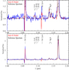 |
Fig. 9. Lower panel: GRAVITY spectrum from 2.0 μm to 2.2 μm (blue-solid line) with a vertical scale that displays the complete line profiles. Upper panel: magnification of the GRAVITY spectrum, where the fine details of our best-fit model (red-dashed line) and of the reference spectrum derived with the stellar parameters from Groh et al. (2012a) (black-dashed line) are appreciated. Notice that the He I 2s-2p and He I 3p-4s are only matched by our hotter red model. |
However, this scenario is not fully consistent with all the observational evidence and theoretical predictions. The hydrodynamic simulations of the wind-wind collision zone, created by Madura et al. (2013), suggest that, instead of an extreme decrease of the ηA mass-loss rate, changes in η Car’s ultra-violet, optical, and X-ray light curves, as well as of the spectral features, are due to slight changes in the wind-wind collision cavity opening angle in combination with a moderate change in the mass-loss rate.
Moreover, when comparing our CMFGEN model with our complementary FEROS optical spectrum (λ4200–7100 Å), we noticed that it is not able to reproduce the metallic [Fe II] and Si II lines, while the cooler Groh model reproduces them (see Fig. F.1). Similar behavior is observed for other previous models that include low primary mass-loss rates close to ∼10−4 M⊙ yr−1 (see e.g., Fig. 12 in Madura et al. 2013). This speaks against the strong decrement in the mass-loss rate obtained by our CMFGEN model, and highlights that ηB plays a major role in the formation of the observed lines in the GRAVITY spectrum. The effects of the secondary and the wind-wind collision zone on the formation of Brγ and He I cannot be reflected by our 1D non-LTE single star model. Nevertheless, they can be investigated with aperture-synthesis images.
For a better understanding of the system’s geometry and how ηB could change the parameters derived by our CMFGEN model, we show in Fig. 10 the line-forming regions of our best-fit model and of the reference one as a function of radius for He I 2s-2p (top panel) and Brγ (lower panel). The vertical black lines indicate the following reference points: (a) the red-dotted line shows the location of photosphere of ηA, which is not equal to the hydrostatic radius (because of its optically thick wind) but to the point where the optical depth τ = 2/3; (b) the black-solid line shows the mean angular resolution limit of the GRAVITY observations (∼2 mas); (c) and the black-dashed line marks the expected projected position of ηB at the time of apastron.
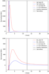 |
Fig. 10. CMFGEN normalized line equivalent width (EW) as a function of radius for our best-fit model and the reference one. Top and bottom panels: line-forming region as a function of radius for He I 2s-2p and Brγ, respectively. The red/blue dotted line corresponds the location of the ηA’s photosphere. The black-solid line indicates the spatial resolution limit of GRAVITY and the black-dashed line shows the projected position of ηB at apastron, according with the mean orbital solution presented by Teodoro et al. (2016). |
With our CMFGEN model, the wind of ηA could form the peak of the Brγ emission only at 3 mas (7 au), which is clearly closer than the extended emission observed in the reconstructed images. Furthermore, it can be seen that, with a single star, the peak of the He I 2s-2p line is formed at an angular scale close the resolution of our observations (in the reference model, the He I line-formation region is at a scale smaller than the resolution of GRAVITY). Therefore, the extended emission in the He I 2s-2p images should be related to the UV ionization of ηB on the wind-wind collision zone. Any modification to He I as a consequence of the wind-wind interaction would require that (i) ηB’s wind penetrates deeply into the denser regions of the primary wind and/or (ii) that ηB ionizes part of the pre- and post-shock primary wind near the apex of the wind-wind collision zone. In this scenario, it is expected that the modification of the ionization structure caused by the secondary largely changes the intensity of Helium and Hydrogen lines depending on the orbital phase, particularly at periastron (see e.g., Groh et al. 2010a; Richardson et al. 2015, 2016).
We do not detect any significant differences in the line profiles between the 2016 and 2017 GRAVITY spectra. However, when comparing the 2016 GRAVITY data and the 2004 AMBER data reported by Weigelt et al. (2007) (both of them obtained at a similar orbital phase), we noticed that the He I 2s-2p shows the P-Cygni profile, but the amplitudes of the valley and peak are different for both data sets. This observation suggests the presence of a dynamical wind-wind collision environment with possible changes in the wind parameters over time (see e.g., Fig. 3 in Richardson et al. 2016, where the P-Cygni profile of He I λ5876 is observed close to several periastron passages but the profile of the line varies with time even for similar phases).Therefore, this highlights the importance of monitoring the lines’ morphological changes through the reconstructed interferometric images.
4.2. The size of η Car’s continuum emission
The observed quiescent continuum emission in η Car is caused by extended free-free and bound-free emission (Hillier et al. 2001), and it traces the dense, optically thick primary wind. From our geometrical model to the Fringe Tracker data, we estimated that ∼50% of the K-band total flux corresponds to θFWHM = 2 mas (∼5 au) core (compact emission), with the rest of the flux arising from a surrounding halo of at least θFWHM = 10 mas (∼24 au; see Table 1). The size derived for the continuum ηA wind is consistent with the size of the extended primary photosphere, according with our CMFGEN model and previous spectroscopic and interferometric estimates (Hillier et al. 2001, 2006; Kervella et al. 2002; van Boekel et al. 2003; Weigelt et al. 2007, 2016).
Previous interferometric studies suggested an elongated continuum primary wind along the PA of the Homunculus. From our data modeling, we derived an elongation ratio of ϵ = 1.06 ± 0.05, a value that is consistent with the most recent interferometric measurements with AMBER, but it is 4−σ smaller than the first VINCI estimate in 2003 (see Table 3). It has been hypothesized that the origin of this elongation could be (i) a latitude-dependent wind caused by a rapid rotation of the primary and/or (ii) a consequence of the wind-wind collision cavity. For example, Mehner et al. (2014) suggest that the angular momentum transfer between ηA and ηB at periastron could be affected by tidal acceleration, resulting in a change of the rotation period of ηA, which in turn may affect the shape of the continuum emission.
Values of η Car’s continuum elongation ratio from different interferometric observations.
Additionally, Groh et al. (2010a) used radiative transfer models applied to the VINCI and AMBER data to explore the changes in the continuum associated with modifications in the rotational velocity and with a “bore-hole” effect due to the presence of the wind-wind collision zone. These authors found that both prolate or oblate rotational models reproduce the interferometric signatures. Nevertheless, those models required large inclination angles in which ηA’s rotational axis is not aligned with that of the Homunculus. Inclinations where the rotational axis is aligned with the Homunculus would require a decrement in the rotational velocity (and of the size) of ηA with time. However, the cavity could also mimic the effects of the observed elongation. Therefore, new radiative transfer models of interferometric data (including GRAVITY and other wavelengths like PIONIER in the H-band) are necessary to test these scenarios. Such models are beyond the scope of the present work and are left for future analysis.
4.3. The Brγ interferometric images in the context of the η Car wind-wind collision cavity
Our 2016 GRAVITY Brγ aperture-synthesis images reveal the morphology of η Car’s wind-wind collision cavity. Here, we discuss the principal wind components and their interpretation with previous theoretical models and simulations. The Brγ maps reveal the following general structure as function of the radial velocity:
(1) Continuum wind region. For radial velocities smaller than −510 km s−1 and larger than +368 km s−1, the maps show a compact emission where the optically thick continuum wind region is dominant. For velocities between −510 km s−1 and +368 km s−1, additional wind components are observed in the images, however, the continuum emission is always present.
(2) Wind-wind collision region. 3D smoothed particle hydrodynamic models (Okazaki et al. 2008; Gull et al. 2009; Madura et al. 2012, 2013; Teodoro et al. 2013, 2016) of η Car’s wind-wind interaction suggest a density distribution that extends far beyond the size of the primary wind. This wind-wind collision zone is identified with a cavity created by the fast wind of ηB that penetrates deep into the dense but slow wind of ηA as the secondary changes its orbital phase. Following the orbital solution of Teodoro et al. (2016) presented in Fig. 1, ηB was close to apastron (in front of ηA) at the time of our GRAVITY observations. Figure 11 displays a schematic view of this wind-wind scenario according to Madura et al. (2013). The diagram represents the position of the system at apastron in a plane defined by the LOS and the sky plane (i.e., called the xz plane in Madura et al. 2013). The cavity opens with a LOS oriented preferably toward the southern wall, along its walls the hot (T ∼ 106 K) post-shock ηB wind is moving, and, in between, the cold (T ∼ 104 K) pre-shock ηB wind is observed.
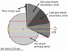 |
Fig. 11. Schematic of η Car’s wind-wind collision scenario reported by Madura et al. (2013). The wind-wind collision cavity carved by the secondary (green star) in the primary wind is depicted, with the different elements of the primary (blue star) and secondary winds labeled. Notice how the LOS lies preferentially toward the lower cavity wall. The angular scales (centered around ηA) traced with the shortest baselines of the GRAVITY (∼40 m) and AMBER (∼10 m) data are shown with a yellow-dashed and red-dotted rectangles, respectively. |
In the Brγ GRAVITY images at radial velocities >−364 km s−1, we observe an extended asymmetric emission increasing in size and brightness as we approach the systemic velocity, and then it decreases toward positive ones. At velocities between −364 km s−1 and −71 km s−1, the wind-wind collision cavity presents an elongated and asymmetric cone-like morphology with a bright arc-like feature in the southeast direction. The extended and bright southeast asymmetric emission was first observed in the AMBER images reported by Weigelt et al. (2016). In particular, for velocities between −140 km s−1 and −380 km s−1, those authors identified a SE fan-shaped morphology. However, there are some changes between the AMBER images and the maps recovered with GRAVITY. We infer that some of those changes are associated with the dynamics of the wind-wind collision zone (i.e., different orbital phases), however, some others are caused by the different spatial frequencies sampled with the two observations.
The majority of the longest baselines of the AMBER data are of 80 m, which limits the angular resolution up to λ/2Bmax = 3 mas, in contrast our GRAVITY data provide a mean maximum angular resolution of 2.26 mas. However, the AMBER data include a better sampling of low spatial frequencies with baselines as small as 10 m. In this respect, our GRAVITY data present a clear limitation since most of our short baselines are above 40 m. Those constraints allowed us to recover images of the small-scale structure of η Car, at the cost of restricting the imaging capabilities to map the most extended emission observed in the AMBER images.
Madura et al. (2013) suggested that the time-dependent changes in the spectral lines are a consequence of changes in the line-of-sight morphology of the wind-wind collision cavity. Their hydrodynamical simulations predict that, at apastron, the cavity maintains an axisymmetric conical shape with the leading and trailing arms clearly visible in the orbital plane4. The half-opening angle of the cavity depends on the ratio of the wind momenta, which can be expressed in terms of mass-loss rate and wind velocity (β = ṀηA vηA/ṀηB vηB), of the two interacting stars. Therefore, any modification to the mass-loss rates and/or wind velocities would change the opening angle of the cavity. For example, ṀηA = 8.5 × 10⁻⁴ M⊙ yr−1 would produce a half-opening angle close to 55°. On the other hand, ṀηA = 1.6 × 10⁻⁴ M⊙ yr−1 would create a half-opening angle close to 80°.
As ηB moves from apastron (lower-left panel in Fig. 12) toward the periastron, the wind-wind cavity is distorted, creating a spiral (lower-middle panel in Fig. 12). Interesting is the phenomenology after the periastron passage, where the leading arm of the cavity collides with the “old” trailing arm, forming a dense, cold, and compressed “shell” of ηA’s wind (lower-right panel in Fig. 12). Since the secondary wind is providing pressure from the direction of the binary, but because of the very high velocity, the shell is expanding outward through the low-density region on the far (apastron) side, the expansion velocity could reach values larger than the terminal velocity of ηA’s wind (v∞ = 420 km s−1). The stability and size of the compressed ηA shells are also dependent on the adopted ṀηA. Bordering the compressed shell of primary wind, there is the hot post-shock ηB wind. Due to the increment of orbital speed of ηB as it approaches the periastron, the post-shock ηB wind is heated to higher temperatures (T ∼ 106 K) than the gas in the trailing arm (T ∼ 104 K), producing an asymmetric hot shock. After the periastron, photo-ablation of the post shock ηA wind could stop the ηB wind from heating the primary wind, enhancing the asymmetric temperature in the inter-cavity between the secondary and (bordering) the compressed shell of primary wind.
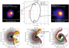 |
Fig. 12. Upper-middle panel: projected orbit of ηB around ηA, with the position of the periastron, apastron, and two imaging epochs labeled on it. Upper-right panel: AMBER map at −277 km s−1, where the fan-shaped SE morphology is observed at ϕ∼ 0.91. Upper-left panel: GRAVITY image at −291 km s−1, the SE arc-like feature is observed at ϕ ∼ 1.28. The FOV of the images is of 36 mas, and they are oriented with the east pointing toward the left and the north toward the top of frames. Lowermost panels: three orbital phases, ϕ = 0.5 (lower-left), ϕ = 1.0 (lower-middle) and ϕ = 1.1 (lower-right), of the wind-wind collision model created by Madura et al. (2013). The panels show the structure of the wind-wind cavity in the orbital plane. The red lines indicate the contour where the density is 10−16 g cm−3 and they highlight the changes in the leading and trailing arms of the wind-wind cavity. The positions of the primary and secondary for each phase are marked on the panels with blue and green dots, respectively. The green, magenta, and yellow areas trace the hot (T ∼ 106 − 108 K) post-shock secondary wind bordering the cavity shells. The vector of the observer’s line-of-sight is labeled on each panel, and it corresponds to ω = 243° and ω = 47°. The principal components‘ of the wind-wind cavity are also indicated in the panels. The lowermost panels were taken from Madura et al. (2013) and adapted to the discussion presented in Sect. 4.3. |
In this framework, the 2016 GRAVITY images reveal the structure of the cavity at an orbital phase ϕ∼ 1.35 (upper-left panel in Fig. 12), where the arc-like feature could be interpreted as the inner-most hot post-shock gas flowing along the cavity walls that border the compressed ηA wind shell in our line-of-sight. The fact that we observe material preferentially along the SE cavity walls, suggests that the half-opening angle is quite similar to the inclination angle of the system.
Madura et al. (2013) shows detailed model snap-shots that illustrate the dependence of the opening angle on the mass-loss rate. However, a straight-forward estimate following the two-wind interaction solution of Canto et al. (1996), keeping constant the secondary mass-loss rate and wind velocities, suggests that a primary mass-loss rate between 5.8 × 10⁻⁴ and 1.2 × 10⁻³M⊙ yr−1 is necessary to produce a half-opening angle in the cavity of 40°–60°. Smaller mass-loss rates would produce bigger angles, which would prevent the wall of the wind-wind collision cavity from intercepting the LOS. The orientation of the extended emission is also consistent with a prograde motion of the secondary (i.e., i > 90°, ω > 180°), with a leading arm projected motion from east to west.
Our analysis of the Brγ arc-like feature’s peak in the 2016 images suggests that not all the material is moving at the same speed, Fig. 13 displays the centroid position (flux centroid of the 90% emission peak) of the arc-like feature versus radial velocity. As it is observed, the centroid distribution varies between 3.0 and 4.0 mas (7–9 au) and between −1.5 and −3.0 mas (3.5–7 au) in RA and Dec, respectively. This indicates that the observed material has a clumpy structure that is not expanding at the same speed. It is also consistent with the hydrodynamic simulations which suggest that the stability of the shells depends on the shock thickness and that fragmentation begins later the higher the value of the primary’s mass-loss rate.
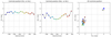 |
Fig. 13. The image displays the centroid position of the 2016 arc-like feature vs. velocity. Left panel: centroid changes in RA vs. velocity. Middle panel: centroid changes in Dec vs. velocity. Right panel: 2D centroid position relative to the ηA’s continuum marked at origin with a blue star. |
Furthermore, it also provides a plausible explanation for the structures observed in the 2014 AMBER images (Weigelt et al. 2016), which correspond to a later orbital phase previous to the periastron passage (upper-right panel in Fig. 12), where the shells are disrupted and the hot ηB wind has already mixed with some portions of the compressed ηA wind. In this scenario the bar, observed in the AMBER data between −414 and −352 km s−1, could be part of the highest velocity component of the hot gas around the distorted shell, while the two antennas of the fan-like structure (from −339 to −227 km s−1) could trace portions of the shell that are not yet fragmented. The SE extended emission at lower negative velocities could be interpreted as part of the material bordering the disrupted shell. The observed extended SW emission at positive velocities could be identified as the material flowing along the leading arm’s wall which is moving away from the observer at the orbital phase of the AMBER images.
This scenario agrees with observations of the fossil shells on larger spatial scales. Teodoro et al. (2013) observed three progressive shells using HST [Fe II] and [Ni II] spectroimages. Since the emission of the forbidden lines is optically thin, the observed shells in the [Fe II] and [Ni II] images support a future radio mapping with ALMA in Hα lines at an angular resolution better than 0.1″ to properly constrain their emmitting regions. The positions of the arcs are consistent with the SE extended emission observed in the interferometric images, but the HST arcs extend up to 0.5″. Those authors derived a time difference between the arcs of the order of the orbital period (∼5.54 years), suggesting that each one was created during a periastron passage. Assuming a constant shell velocity, Teodoro et al. (2013) derived a traveling speed of the fossil shells of +475 km s−1, with the closest arc to ηA located, in projection, at ∼0.1″ (235 au). Notice that the innermost arc presented in Fig. 2 of Teodoro et al. (2013) resembles the fan-like structure observed in the AMBER images.
It is important to highlight that, while the HST images are tracing the compressed ηA wind in the fossil shells, our Brγ images are tracing the hot gas, bordering them, along the cavity walls. A monitoring of the arc-like features with GRAVITY (using short baselines) will be fundamental to characterize the primary’s mass-los rate and the effect of ηB over the primary wind shells over future orbital phases.
4.4. Ionization effect of ηB’s wind observed through the He I 2s-2p line
Helium lines are one of the most intriguing spectral features in η Car’s spectrum. For example, the discovery of the binary was in part based on spectroscopic variations of the H-band He I lines (Damineli 1996; Damineli et al. 1997). Since then, several authors have studied the variations in the helium profiles as a consequence of a binary signature (Groh & Damineli 2004; Nielsen et al. 2007; Humphreys et al. 2008; Damineli et al. 2008b; Mehner et al. 2010, 2012). The different CMFGEN models support that the helium lines could be originated in the densest wind of ηA. Depending on the Ṁ used, the line-emitting region could be extended from a few au to several hundred au (Hillier et al. 2001, 2006; Groh et al. 2012a, see also Sect. 4.1).
However, these models do not fully reproduce the observed evolution of the He I lines without considering the role of ηB (see e.g., Nielsen et al. 2007; Damineli et al. 2008b). It is still not clear where and how the Helium lines are formed in the wind-wind collision scenario. Humphreys et al. (2008), based on HST observations, suggested that the He I lines originate at spatial scales smaller than 100–200 au (∼40–80 mas), but still the structure of the line-formation region was not indicated. The recent 3D hydrodynamic simulations of Clementel et al. (2015a, b) presented maps of the different ionization regions (He0+, He+, He2+) at the innermost 155 au of η Car’s core. These simulations take into account the ionization structure of ηA’s wind and the effect of ηB’s wind on the collision region for the three different mass-loss rates studied in Madura et al. (2013). These models show that there are several regions composed by He+ that might be responsible for the changes observed in the He I profiles.
The GRAVITY observations presented in this study allowed us to obtain the first milliarcsecond resolution images of the inner 20 mas (50 au) He I 2s-2p line-emitting region. In contrast to Brγ, which is observed purely in emission, He I 2s-2p shows a P-Cygni profile with the absorption side blue-shifted. This profile is similar to the helium lines observed at other wavelengths (see e.g., Nielsen et al. 2007). In our images, at velocities between −403 and −326 km s−1, which correspond to the valley of the line, the extended emission is brighter than at other wavelengths. As we move from the valley to the peak of the line, the brightness of the extended emission decreases, slightly increasing again at velocities around the line’s peak (between −95 and −18 km s−1). At the red-shifted velocities, the continuum is dominant and the extended component is marginally observed at low-velocities. At the valley of the line, the 2016 images show an elongated emission that is oriented at a PA ∼ 130° and it extends on both sides of the continuum, with the southeast side slightly more extended.
To compare the morphological changes observed in the images with the model developed by Clementel et al. (2015a, b), we use an adapted version of the helium distribution presented in Fig. 8 by Clementel et al. (2015b). The schematic diagram, in Fig. 14 displays the distribution of helium, in the inner 155 au of η Car. Region 1 corresponds to the zone in the primary wind that is composed mostly by He0+. Region 2 shows the hot post-shock ηB’s wind composed mostly by fully ionized He2+. Regions 3–6 correspond to the zones composed by He+ and region 7 displays the borders of the cavity walls where compressed post-shock ηA’s wind is found.
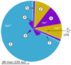 |
Fig. 14. Different He ionized regions: He0+ (blue), He+ (purple), He2+ (yellow). The sketch is oriented in a plane parallel to the line-of-sight and the sky plane. Different regions in the wind-wind collision scenario are labeled. Region 1 represents the He0+ zone in the primary wind. Region 2 shows the hot post-shock secondary wind composed by He2+. Regions 3–6 correspond to the zones composed by He+ in the primary and secondary winds. Region 7 displays the borders of the cavity walls. |
From the distribution of He+, four main regions are observed at different morphological scales. The first of them (region 3) corresponds to the pre-shock primary wind that is partially ionized only by ηA. The second zone (region 4) is created by the He0+-ionizing photons from ηB’s wind that penetrate the pre-shock primary wind. This region varies in size, being more compact along the azimuthal plane than in the orbital one. Clementel et al. (2015b) argued as possible cause for these differences the less turbulent nature of the wind-wind interaction region in the azimuthal plane. Region 5 shows the He+, of the post-shock wind of ηA, trapped in the walls of the cavity. Finally, region 6 displays the section of the pre-shock ηB wind with He+. It is important to highlight that regions 3–5 are expected to be around three orders of magnitude denser than region 6.
The fact that we observe the absorption side of the He I 2s-2p blue-shifted implies that it is formed by material in front of ηA. It means that regions 4–6 are in the LOS. Therefore, the He I 2s-2p structure observed in the GRAVITY images is formed by the different contribution of those regions. By analyzing the images, we hypothesized that the elongated structure, at velocity channels near the valley of the line, appears to be formed by the emission coming mainly from regions 4 and 5. This idea is consistent with the flow of the He+ pre-shock primary wind, coming toward us at a velocity of ∼ −400 km s−1, near the apex of the wind-wind collision zone.
This effect could explain why we observe the most prominent emission at large velocity channels between −403 and −326 km s−1. Given the PA of the observer’s LOS and the orbital plane, we expect to observe emission coming from region 4 at the top and bottom of the continuum. This scenario is also consistent with the emission observed in the GRAVITY images. Since the system near apastron is preferentially oriented toward the material in region 4 that borders the lower wall of the cavity, we also expect to observe an asymmetric emission as the one detected in the images.
As we move toward the systemic velocity of the line, we notice that the extended emission decreases in brightness and size, but it increases again at velocity channels near the emission peak. We suspect that this effect is caused by the material in region 5. The post-shock primary wind in the thin walls of the cavity experiences a turbulent environment, particularly at the apex, that causes some of the material to have zero or positive radial velocities. Notice, however, that for velocities larger than +98 km s−1, the main source of the emission is within the size of the primary beam. This suggests that the origin of large red-shifted velocities is the pre-shock ionized wind from ηA (region 3). Hence, similar to Brγ, the observed spatial distribution of He is in agreement with Clementel et al. (2015a) models with ṀηA close to 10−3M⊙ yr−1. However, future, new hydrodynamic models of the He I 2s-2p line in addition to a GRAVITY monitoring of the line’s morphology are necessary to provide solid constraints on the mass-loss rate of the system.
5. Conclusions
-
We present GRAVITY interferometric data of η Car’s core. Our observations trace the inner 20 mas (50 au) of the source at a resolution of 2.26 mas. The spectro-interferometric capabilities of GRAVITY allowed us to chromatically image Brγ and He I 2s-2p emission regions with a spectral resolution of R = 4000, while the analysis of the Fringe Tracker data allowed us to measure the size of the continuum emission, and the integrated spectrum to characterize the parameters of the primary star.
-
From our geometrical model of the Fringe Tracker squared visibilities, we constrained the size of the continuum emission. We derived a mean FWHM angular scale of 2 mas (∼5 au) and an elongation ratio ϵ = 1.06 ± 0.5 for the compact continuum emission of ηA, together with an extended over-resolved emission with an angular size of at least 10 mas. These estimates are in agreement with previous interferometric measurements. Some of the plausible hypotheses to explain the observed elongation of the continuum compact emission are the fast rotation of the primary and/or the effect of the wind-wind collision cavity. A future monitoring of the continuum size and elongation with GRAVITY and other interferometric facilities at different wavelengths, in combination with radiative transfer models, would serve to test these scenarios.
-
To characterize the properties of ηA’s wind, we applied a CMFGEN 1D non-LTE model to the GRAVITY spectrum. Our model reproduces the He I 2s-2p and He I 3p-4s lines, which could not be formed with the parameters used in previous models in the literature. However, the line-emitting regions of the best-fit model are quite small compared to the structure observed in the reconstructed images. These results imply that single-star models are not enough to reproduce all the observational data. Therefore, the role of ηB should be taken into account when modeling the η Car spectrum. Furthermore, when comparing our model with the η Car spectrum in the visible, we could not reproduce the observed metallic features. We suspect that this is caused because many of the metallic lines are forbidden lines with critical electron densities of 107 − 8 cm−3. With the FEROS aperture, this emission is originating in the fossil wind shells and hence not reproduced in the stellar model.
-
Our aperture-synthesis images allowed us to observe the inner wind-wind collision structure of η Car. Previous AMBER interferometric images of Brγ revealed the wind-wind collision cavity produced by the shock of the fast ηB’s wind with the slow and dense ηA’s wind. Our new 2016 GRAVITY Brγ images show the structure of such cavity at a different orbital phase with a 2.26 mas resolution. The observed morphologies in the images are (qualitatively) in agreement with the theoretical hydrodynamical models of Madura et al. (2013). Particularly interesting is the bright SE arc-like feature, which could be interpreted as the hot post-shock gas flowing along the cavity wall (oriented toward the observer) that border the innermost shell of compressed primary wind, which is formed by the shock of the cavity’s trailing arm with the leading arm after the most recent periastron passage.
-
Due to the sparseness of the 2017 GRAVITY data the quality of the reconstructed images from this epoch is clearly affected. Therefore, those images could not be used for a direct comparison with the 2016 ones. Nevertheless, our analysis of the interferometric observables, in coincidental baselines, reveals changes in the cavity structure. The ulterior characterization of those changes is subject to future imaging epochs with a less limited u−v coverage than the 2017 data.
-
We presented, the first images of the He I 2s-2p line. They were qualitatively interpreted using the model of Clementel et al. (2015a,b). We hypothesized that the observed emission is coming mainly from the He+ at the cavity walls and from a portion of the pre-shock primary wind ionized by the secondary. From the size of the observed emission and the theoretical models, we suspect that the mass-loss rate of the primary is close to 10−3 M⊙ yr−1. The emission observed require an active role of ηB to ionize the material near the apex of the wind-wind collision cavity.
-
Spectro-interferometric imaging cubes offer us unique information to constrain the wind parameters of η Car, not accessible by other techniques. In this study, we have shown the imaging capabilities of GRAVITY to carry out this task. A future monitoring of η Car over the orbital period (particularly at the periastron passage), in combination with dedicated hydrodynamical models of the imaged K-band lines, will provide a unique opportunity to constrain the stellar and wind parameters of the target, and, ultimately, to predict its evolution and fate.
For a complete description of the changes in the wind-wind collision cavity and their 3D orientation at scales relevant to the interferometric images, we refer the reader to Figs. 1, 2, B1, B2, B3 and B4 in Madura et al. (2013).
Here, we adopted the 2009 periastron passage, T0 = 2454851.7 JD, as reference for the orbital phases labeled on the reconstructed images and diagrams of the wind-wind cavity structure.
Acknowledgments
We thank the anonymous referee for his/her comments to improve this work. J.S.B acknowledges the support from the Alexander von Humboldt Foundation Fellowship program (Grant number ESP 1188300 HFST-P) and to the ESO Fellowship program. The work of A.M. is supported by the Deutsche Forschungsgemeinschaft priority program 1992. A.A., N.A. and P.J.V.G. acknowledge funding from Fundação para a Ciência e a Tecnologia (FCT) (SFRH/BD/52066/2012; PTDC/CTE-AST/116561/2010; UID/FIS/00099/2013) and the European Commission (Grant Agreement 312430, OPTICON).
References
- Allard, F., Homeier, D., & Freytag, B. 2012, Phil. Trans. R. Soc. London, Ser. A, 370, 2765 [Google Scholar]
- Allen, D. A., & Hillier, D. J. 1993, Proc. Astron. Soc. Aust., 10, 338 [NASA ADS] [CrossRef] [Google Scholar]
- Asplund, M., Grevesse, N., Sauval, A. J., Allende Prieto, C., & Blomme, R. 2005, A&A, 431, 693 [NASA ADS] [CrossRef] [EDP Sciences] [Google Scholar]
- Baron, F., & Kloppenborg, B. 2010, SPIE Conf. Ser., 7734, 4 [Google Scholar]
- Blind, N., Eisenhauer, F., Haug, M., et al. 2014, Proc. SPIE, 9146, 91461U [Google Scholar]
- Brahm, R., Jordán, A., & Espinoza, N. 2017, PASP, 129, 034002 [NASA ADS] [CrossRef] [Google Scholar]
- Canto, J., Raga, A. C., & Wilkin, F. P. 1996, ApJ, 469, 729 [NASA ADS] [CrossRef] [Google Scholar]
- Clementel, N., Madura, T. I., Kruip, C. J. H., & Paardekooper, J.-P. 2015a, MNRAS, 450, 1388 [NASA ADS] [CrossRef] [Google Scholar]
- Clementel, N., Madura, T. I., Kruip, C. J. H., Paardekooper, J.-P., & Gull, T. R. 2015b, MNRAS, 447, 2445 [NASA ADS] [CrossRef] [Google Scholar]
- Conti, P. S. 1984, IAU Symp., 105, 233 [Google Scholar]
- Conti, P. S., & Niemelä, V. S. 1976, ApJ, 209, L37 [NASA ADS] [CrossRef] [Google Scholar]
- Corcoran, M. F. 2005, AJ, 129, 2018 [NASA ADS] [CrossRef] [Google Scholar]
- Corcoran, M. F., Hamaguchi, K., Pittard, J. M., et al. 2010, ApJ, 725, 1528 [NASA ADS] [CrossRef] [Google Scholar]
- Damineli, A. 1996, ApJ, 460, L49 [NASA ADS] [CrossRef] [Google Scholar]
- Damineli, A., Conti, P. S., & Lopes, D. F. 1997, New Astron., 2, 107 [NASA ADS] [CrossRef] [Google Scholar]
- Damineli, A., Hillier, D. J., Corcoran, M. F., et al. 2008a, MNRAS, 386, 2330 [NASA ADS] [CrossRef] [Google Scholar]
- Damineli, A., Hillier, D. J., Corcoran, M. F., et al. 2008b, MNRAS, 384, 1649 [NASA ADS] [CrossRef] [Google Scholar]
- Davidson, K., & Humphreys, R. M. 1997, ARA&A, 35, 1 [NASA ADS] [CrossRef] [Google Scholar]
- Davidson, K., Gull, T. R., & Ishibashi, K. 2001, ASP Conf. Ser., 233, 173 [NASA ADS] [Google Scholar]
- Davidson, K., Mehner, A., Humphreys, R. M., Martin, J. C., & Ishibashi, K. 2015, ApJ, 801, L15 [NASA ADS] [CrossRef] [Google Scholar]
- Duvert, G., Young, J., & Hummel, C. 2017, A&A, 597, A8 [NASA ADS] [CrossRef] [EDP Sciences] [Google Scholar]
- Eisenhauer, F., Perrin, G., Brandner, W., et al. 2008, SPIE Conf. Ser., 7013, 70132A [Google Scholar]
- Eisenhauer, F., Perrin, G., Brandner, W., et al. 2011, The Messenger, 143, 16 [NASA ADS] [Google Scholar]
- Falcke, H., Davidson, K., Hofmann, K.-H., & Weigelt, G. 1996, A&A, 306, L17 [NASA ADS] [Google Scholar]
- Gillessen, S., Eisenhauer, F., Perrin, G., et al. 2010, SPIE Conf. Ser., 7734, 77340Y [Google Scholar]
- Glindemann, A., Algomedo, J., Amestica, R., et al. 2003, SPIE Conf. Ser., 4838, 89 [NASA ADS] [CrossRef] [Google Scholar]
- Gomez, H. L., Vlahakis, C., Stretch, C. M., et al. 2010, MNRAS, 401, L48 [NASA ADS] [CrossRef] [Google Scholar]
- Gravity Collaboration (Abuter, R., et al.) 2017, A&A, 602, A94 [NASA ADS] [CrossRef] [EDP Sciences] [Google Scholar]
- Groh, J. H., & Damineli, A. 2004, IBVS, 5492 [Google Scholar]
- Groh, J. H., Madura, T. I., Owocki, S. P., Hillier, D. J., & Weigelt, G. 2010a, ApJ, 716, L223 [NASA ADS] [CrossRef] [Google Scholar]
- Groh, J. H., Nielsen, K. E., Damineli, A., et al. 2010b, A&A, 517, A9 [NASA ADS] [CrossRef] [EDP Sciences] [Google Scholar]
- Groh, J. H., Hillier, D. J., Madura, T. I., & Weigelt, G. 2012a, MNRAS, 423, 1623 [NASA ADS] [CrossRef] [Google Scholar]
- Groh, J. H., Madura, T. I., Hillier, D. J., Kruip, C. J. H., & Weigelt, G. 2012b, ApJ, 759, L2 [NASA ADS] [CrossRef] [Google Scholar]
- Gull, T. R., Nielsen, K. E., Corcoran, M. F., et al. 2009, MNRAS, 396, 1308 [NASA ADS] [CrossRef] [Google Scholar]
- Gull, T. R., Madura, T. I., Groh, J. H., & Corcoran, M. F. 2011, ApJ, 743, L3 [NASA ADS] [CrossRef] [Google Scholar]
- Gull, T. R., Madura, T. I., Teodoro, M., et al. 2016, MNRAS, 462, 3196 [NASA ADS] [CrossRef] [Google Scholar]
- Hillier, D. J., & Miller, D. L. 1998, ApJ, 496, 407 [NASA ADS] [CrossRef] [Google Scholar]
- Hillier, D. J., Davidson, K., Ishibashi, K., & Gull, T. 2001, ApJ, 553, 837 [NASA ADS] [CrossRef] [Google Scholar]
- Hillier, D. J., Gull, T., Nielsen, K., et al. 2006, ApJ, 642, 1098 [NASA ADS] [CrossRef] [Google Scholar]
- Hofmann, K.-H., & Weigelt, G. 1988, A&A, 203, L21 [NASA ADS] [Google Scholar]
- Humphreys, R. M., & Davidson, K. 1994, PASP, 106, 1025 [NASA ADS] [CrossRef] [Google Scholar]
- Humphreys, R. M., Davidson, K., & Koppelman, M. 2008, AJ, 135, 1249 [NASA ADS] [CrossRef] [Google Scholar]
- Kaufer, A., & Pasquini, L. 1998, Proc. SPIE, 3355, 844 [NASA ADS] [CrossRef] [Google Scholar]
- Kervella, P., Coudé du Foresto, V., Glindemann, A., & Hofmann, R. 2000, SPIE Conf. Ser., 4006, 31 [NASA ADS] [CrossRef] [Google Scholar]
- Kervella, P., Schöller, M., van Boekel, R., et al. 2002, ASP Conf. Ser., 279, 99 [NASA ADS] [Google Scholar]
- Langer, N. 1998, A&A, 329, 551 [NASA ADS] [Google Scholar]
- Langer, N., Hamann, W.-R., Lennon, M., et al. 1994, A&A, 290, 819 [NASA ADS] [Google Scholar]
- Lapeyrere, V., Kervella, P., Lacour, S., et al. 2014, SPIE Conf. Ser., 9146, 91462D [Google Scholar]
- Madura, T. I., & Groh, J. H. 2012, ApJ, 647, L18 [NASA ADS] [CrossRef] [Google Scholar]
- Madura, T. I., Gull, T. R., Owocki, S. P., et al. 2012, MNRAS, 420, 2064 [NASA ADS] [CrossRef] [Google Scholar]
- Madura, T. I., Gull, T. R., Okazaki, A. T., et al. 2013, MNRAS, 436, 3820 [NASA ADS] [CrossRef] [Google Scholar]
- Mehner, A., Davidson, K., Ferland, G. J., & Humphreys, R. M. 2010, ApJ, 710, 729 [NASA ADS] [CrossRef] [Google Scholar]
- Mehner, A., Davidson, K., Humphreys, R. M., et al. 2012, ApJ, 751, 73 [NASA ADS] [CrossRef] [Google Scholar]
- Mehner, A., Ishibashi, K., Whitelock, P., et al. 2014, A&A, 564, A14 [NASA ADS] [CrossRef] [EDP Sciences] [Google Scholar]
- Meynet, G., & Maeder, A. 2003, A&A, 404, 975 [NASA ADS] [CrossRef] [EDP Sciences] [Google Scholar]
- Meynet, G., Georgy, C., Hirschi, R., et al. 2011, Bull. Soc. Roy. Sci. Liège, 80, 266 [Google Scholar]
- Millour, F., Vannier, M., Petrov, R. G., et al. 2006, EAS Pub. Ser., 22, 379 [CrossRef] [Google Scholar]
- Millour, F., Petrov, R. G., Chesneau, O., et al. 2007, A&A, 464, 107 [NASA ADS] [CrossRef] [EDP Sciences] [Google Scholar]
- Morris, P. W., Gull, T. R., Hillier, D. J., et al. 2017, ApJ, 842, 79 [NASA ADS] [CrossRef] [Google Scholar]
- Nielsen, K. E., Ivarsson, S., & Gull, T. R. 2007, ApJs, 168, 289 [NASA ADS] [CrossRef] [Google Scholar]
- Okazaki, A. T., Owocki, S. P., Russell, C. M. P., & Corcoran, M. F. 2008, MNRAS, 388, L39 [NASA ADS] [CrossRef] [MathSciNet] [Google Scholar]
- Parkin, E. R., Pittard, J. M., Corcoran, M. F., Hamaguchi, K., & Stevens, I. R. 2009, MNRAS, 394, 1758 [NASA ADS] [CrossRef] [Google Scholar]
- Parkin, E. R., Pittard, J. M., Corcoran, M. F., & Hamaguchi, K. 2011, ApJ, 726, 105 [NASA ADS] [CrossRef] [Google Scholar]
- Pastorello, A., Botticella, M. T., Trundle, C., et al. 2010, MNRAS, 408, 181 [NASA ADS] [CrossRef] [Google Scholar]
- Patil, A., Huard, D., & Fonnesbeck, C. J. 2010, J. Stat. Softw., 35, 1 [CrossRef] [EDP Sciences] [Google Scholar]
- Pauls, T. A., Young, J. S., Cotton, W. D., & Monnier, J. D. 2005, PASP, 117, 1255 [NASA ADS] [CrossRef] [Google Scholar]
- Petrov, R. G., Malbet, F., Weigelt, G., et al. 2007, A&A, 464, 1 [NASA ADS] [CrossRef] [EDP Sciences] [Google Scholar]
- Pittard, J. M., & Corcoran, M. F. 2002, A&A, 383, 636 [NASA ADS] [CrossRef] [EDP Sciences] [Google Scholar]
- Richardson, N. D., Gies, D. R., Gull, T. R., Moffat, A. F. J., & St-Jean, L. 2015, AJ, 150, 109 [NASA ADS] [CrossRef] [Google Scholar]
- Richardson, N. D., Madura, T. I., St-Jean, L., et al. 2016, MNRAS, 461, 2540 [NASA ADS] [CrossRef] [Google Scholar]
- Sanchez-Bermudez, J., Alberdi, A., Barbá, R., et al. 2017, ApJ, 845, 57 [NASA ADS] [CrossRef] [Google Scholar]
- Smith, N. 2006, MNRAS, 367, 763 [NASA ADS] [CrossRef] [Google Scholar]
- Smith, N. 2007, AIP Conf. Ser., 937, 163 [NASA ADS] [CrossRef] [Google Scholar]
- Smith, N., Bally, J., & Morse, J. A. 2003, ApJ, 587, L105 [NASA ADS] [CrossRef] [Google Scholar]
- Smith, N., Gehrz, R. D., Campbell, R., et al. 2011, MNRAS, 418, 1959 [NASA ADS] [CrossRef] [Google Scholar]
- Steffen, W., Teodoro, M., Madura, T. I., et al. 2014, MNRAS, 442, 3316 [NASA ADS] [CrossRef] [Google Scholar]
- Teodoro, M., Damineli, A., Sharp, R. G., Groh, J. H., & Barbosa, C. L. 2008, MNRAS, 387, 564 [NASA ADS] [CrossRef] [Google Scholar]
- Teodoro, M., Madura, T. I., Gull, T. R., Corcoran, M. F., & Hamaguchi, K. 2013, ApJ, 773, L16 [NASA ADS] [CrossRef] [Google Scholar]
- Teodoro, M., Damineli, A., Heathcote, B., et al. 2016, ApJ, 819, 131 [NASA ADS] [CrossRef] [Google Scholar]
- Trundle, C., Kotak, R., Vink, J. S., & Meikle, W. P. S. 2008, A&A, 483, L47 [NASA ADS] [CrossRef] [EDP Sciences] [Google Scholar]
- van Boekel, R., Kervella, P., Schöller, M., et al. 2003, A&A, 410, L37 [CrossRef] [EDP Sciences] [Google Scholar]
- Walborn, N. R. 1973, ApJ, 179, 517 [NASA ADS] [CrossRef] [Google Scholar]
- Weigelt, G., & Ebersberger, J. 1986, A&A, 163, L5 [NASA ADS] [Google Scholar]
- Weigelt, G., Albrecht, R., Barbieri, C., et al. 1995, Rev. Mex. Astron. Astrofis., 2, 11 [Google Scholar]
- Weigelt, G., Kraus, S., Driebe, T., et al. 2007, A&A, 464, 87 [NASA ADS] [CrossRef] [EDP Sciences] [Google Scholar]
- Weigelt, G., Hofmann, K.-H., Schertl, D., et al. 2016, A&A, 594, A106 [NASA ADS] [CrossRef] [EDP Sciences] [Google Scholar]
Appendix A: GRAVITY observations’ lists
η Car’s 2016 GRAVITY observations.
η Car’s 2017 GRAVITY observations.
Appendix B: Posterior distributions of the best-fit geometrical model
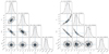 |
Fig. B.1. Posterior distributions of the best-fit parameters of the geometrical model presented in Sect. 3.1. Left panel: posterior distributions for the model applied to the V2 data at PA⊥ = 40° ± 20°, while the right panel displays the posterior distributions for the model at PA∥ = 130° ± 20°. The 2D distributions show 1 and 2 standard deviations encircled with a black contour. The mean of each distribution is displayed with a blue square. The 1D histograms show the expected value (mean) and ±1σ with vertical dashed lines, together with their corresponding values at the top. |
Appendix C: Dirty beams of the GRAVITY imaging epochs
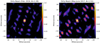 |
Fig. C.1. Dirty beams of the 2016 (left) and 2017 (right) GRAVITY data. Notice the strong secondary lobes caused by the more sparse u−v coverage of the second epoch. |
Appendix D: Reconstructed Brγ and He I images from the 2017 GRAVITY data
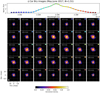 |
Fig. D.1. Brγ interferometric aperture synthesis images from the May-June 2017 data. The Doppler velocity of each frame is labeled in the images. For all the panels, east is to the left and north to the top and the displayed FOV corresponds to 36 × 36 mas. The small white ellipse shown in the lowermost-left panel corresponds to the synthesized beam (the detailed PSF is shown in Fig. D.1). Above all the images, the GRAVITY spectrum is shown and the different positions where the images are reconstructed across the line are labeled with a colored square, which is also plotted in the images for an easy identification. Due to the sparseness of the u−v coverage, the quality of these reconstructed images is limited, creating a clumpy fine structure and a cross-like shape superimposed on the source’s brightness distribution. Therefore, they cannot be properly compared with the GRAVITY 2016 data presented in this work. |
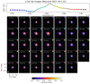 |
Fig. D.2. He I interferometric aperture synthesis images from the May–June 2017 data. The maps are as described in Fig. D.1. |
Appendix E: Best-fit of the reconstructed images to the V2 and closure phases
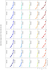 |
Fig. E.1. Fit to the observed V2 from the interferometric aperture synthesis images across the Brγ line (2016). The colored dots correspond to the synthetic V2 extracted from the unconvolved reconstructed images, while the observational data are represented with gray dots with 1σ error-bars. The Doppler velocity is labeled in each panel. All the panels share the same horizontal and vertical scales. |
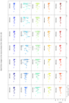 |
Fig. E.2. Fit to the observed closure phases from the interferometric aperture synthesis images across the Brγ line (2016). The panels are as described in Fig. E.1. |
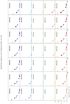 |
Fig. E.3. Fit to the observed V2 from the interferometric aperture synthesis images across the Brγ line (2017). The panels are as described in Fig. E.1. |
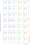 |
Fig. E.4. Fit to the observed closure phases from the interferometric aperture synthesis images across the Brγ line (2017). The panels are as described in Fig. E.1. |
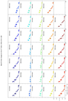 |
Fig. E.5. Fit to the observed V2 from the interferometric aperture synthesis images across the He I line (2016). The panels are as described in Fig. E.1. |
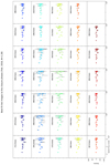 |
Fig. E.6. Fit to the observed closure phases from the interferometric aperture synthesis images across the He I line (2016). The panels are as described in Fig. E.1. |
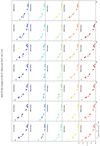 |
Fig. E.7. Fit to the observed V2 from the interferometric aperture synthesis images across the He I line (2017). The panels are as described in Fig. E.1. |
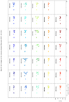 |
Fig. E.8. Fit to the observed closure phases from the interferometric aperture synthesis images across the He I line (2017). The panels are as described in Fig. E.1. |
Appendix F: CMFGEN models of the FEROS η Car spectrum
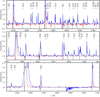 |
Fig. F.1. 2016 η Car’s FEROS spectrum (blue-solid line). The image displays our best-fit CMFGEN model (red-dashed line) and the model described in Groh et al. (2012a; black-dashed line). The Balmer lines of the FEROS spectrum are too strong. They include large contributions of the circumstellar emission as a result of the bad seeing of ∼2″ at the time of the observation. The black synthetic spectrum matches the Fe II and Si II lines. The absorption component of the P-Cygni profiles are filled in and the He I emission lines are not reproduced by the model, which has been already observed and discussed in detail by Hillier et al. (2001). The hotter red model can hardly fit the spectral lines observed at FEROS’ wavelengths. |
All Tables
Values of η Car’s continuum elongation ratio from different interferometric observations.
All Figures
|
Fig. 1. Homunculus Nebula and the binary orbit projected in the plane of the sky (left panel; front view) and in a plane formed by the observer’s LOS and the sky plane (right panel; side view). The 3D Homunculus model was obtained from the online resources of Steffen et al. (2014). |
| In the text | |
|
Fig. 2. η Car’s u−v coverages obtained during the GRAVITY runs in February 2016 (top panel) and May-June 2017 (bottom panel). Different quadruplets are indicated with different colors. |
| In the text | |
|
Fig. 3. 2016 (blue straight line) and 2017 (black straight line) η Car normalized spectra in the 2.0–2.2 μm bandpass. The vertical red-dashed lines indicate the spectral features identified in the spectrum. |
| In the text | |
|
Fig. 4. Normalized GRAVITY spectrum at the position of the He I 2s-2p and Brγ lines. The calibrated differential visibilities (middle) and phases (bottom) of one of the GRAVITY data sets (MJD: 57903.9840) are also shown. In the middle and bottom panels, different colors correspond to each one of the baselines in the data set (see label on the plots). The dashed-red vertical lines indicate the reference wavelength of the emission feature, and the dashed-horizontal lines show the reference value of the continuum baseline. |
| In the text | |
|
Fig. 5. Left panels: best-fit geometrical model to the Fringe Tracker V 2 data. The model is plotted with a black line, the data are shown with blue dots and the model parameters (with their uncertainties) are indicated on each panel. Right panels: visibility points used for each model fitting at two different position angles, PA⊥ = 40°± 20° and PA∥ = 130°± 20°. |
| In the text | |
|
Fig. 6. Brγ interferometric aperture synthesis images from the Feb. 2016 data. The Doppler velocity of each frame is labeled in the images. For all the panels, east is to the left and north to the top. The displayed FOV corresponds to 36 × 36 mas. The small white ellipse shown in the lowermost-left panel corresponds to the synthesized primary beam (the detailed PSF is shown in Fig. D.1). Above all the images, the GRAVITY spectrum is shown and the different positions where the images are reconstructed across the line are labeled with a colored square, which is also plotted in the images for an easy identification. |
| In the text | |
|
Fig. 7. He I interferometric aperture synthesis images from the Feb. 2016 data. The maps are as described in Fig. 6. |
| In the text | |
|
Fig. 8. Differential phases (left panels) and differential visibilities (right panels) between the continuum and the line emission for the 2016 (blue line) and 2017 data (purple line). The (reference) continuum phase and visibility were estimated using the first and last five channels in the imaged bandpass. Each one of the rows corresponds to a similar baseline in both epochs, tracing large (top), intermediate (middle) and small (bottom) spatial scales. The baseline lengths and position angles are labeled on the left panels, while the baseline stations are labeled on the right ones. The black-dashed lines correspond to the differential quantities extracted from the unconvolved reconstructed images. The vertical red-dotted line marks the systemic velocity of Brγ. The horizontal red-dotted lines show the continuum baselines. |
| In the text | |
|
Fig. 9. Lower panel: GRAVITY spectrum from 2.0 μm to 2.2 μm (blue-solid line) with a vertical scale that displays the complete line profiles. Upper panel: magnification of the GRAVITY spectrum, where the fine details of our best-fit model (red-dashed line) and of the reference spectrum derived with the stellar parameters from Groh et al. (2012a) (black-dashed line) are appreciated. Notice that the He I 2s-2p and He I 3p-4s are only matched by our hotter red model. |
| In the text | |
|
Fig. 10. CMFGEN normalized line equivalent width (EW) as a function of radius for our best-fit model and the reference one. Top and bottom panels: line-forming region as a function of radius for He I 2s-2p and Brγ, respectively. The red/blue dotted line corresponds the location of the ηA’s photosphere. The black-solid line indicates the spatial resolution limit of GRAVITY and the black-dashed line shows the projected position of ηB at apastron, according with the mean orbital solution presented by Teodoro et al. (2016). |
| In the text | |
|
Fig. 11. Schematic of η Car’s wind-wind collision scenario reported by Madura et al. (2013). The wind-wind collision cavity carved by the secondary (green star) in the primary wind is depicted, with the different elements of the primary (blue star) and secondary winds labeled. Notice how the LOS lies preferentially toward the lower cavity wall. The angular scales (centered around ηA) traced with the shortest baselines of the GRAVITY (∼40 m) and AMBER (∼10 m) data are shown with a yellow-dashed and red-dotted rectangles, respectively. |
| In the text | |
|
Fig. 12. Upper-middle panel: projected orbit of ηB around ηA, with the position of the periastron, apastron, and two imaging epochs labeled on it. Upper-right panel: AMBER map at −277 km s−1, where the fan-shaped SE morphology is observed at ϕ∼ 0.91. Upper-left panel: GRAVITY image at −291 km s−1, the SE arc-like feature is observed at ϕ ∼ 1.28. The FOV of the images is of 36 mas, and they are oriented with the east pointing toward the left and the north toward the top of frames. Lowermost panels: three orbital phases, ϕ = 0.5 (lower-left), ϕ = 1.0 (lower-middle) and ϕ = 1.1 (lower-right), of the wind-wind collision model created by Madura et al. (2013). The panels show the structure of the wind-wind cavity in the orbital plane. The red lines indicate the contour where the density is 10−16 g cm−3 and they highlight the changes in the leading and trailing arms of the wind-wind cavity. The positions of the primary and secondary for each phase are marked on the panels with blue and green dots, respectively. The green, magenta, and yellow areas trace the hot (T ∼ 106 − 108 K) post-shock secondary wind bordering the cavity shells. The vector of the observer’s line-of-sight is labeled on each panel, and it corresponds to ω = 243° and ω = 47°. The principal components‘ of the wind-wind cavity are also indicated in the panels. The lowermost panels were taken from Madura et al. (2013) and adapted to the discussion presented in Sect. 4.3. |
| In the text | |
|
Fig. 13. The image displays the centroid position of the 2016 arc-like feature vs. velocity. Left panel: centroid changes in RA vs. velocity. Middle panel: centroid changes in Dec vs. velocity. Right panel: 2D centroid position relative to the ηA’s continuum marked at origin with a blue star. |
| In the text | |
|
Fig. 14. Different He ionized regions: He0+ (blue), He+ (purple), He2+ (yellow). The sketch is oriented in a plane parallel to the line-of-sight and the sky plane. Different regions in the wind-wind collision scenario are labeled. Region 1 represents the He0+ zone in the primary wind. Region 2 shows the hot post-shock secondary wind composed by He2+. Regions 3–6 correspond to the zones composed by He+ in the primary and secondary winds. Region 7 displays the borders of the cavity walls. |
| In the text | |
|
Fig. B.1. Posterior distributions of the best-fit parameters of the geometrical model presented in Sect. 3.1. Left panel: posterior distributions for the model applied to the V2 data at PA⊥ = 40° ± 20°, while the right panel displays the posterior distributions for the model at PA∥ = 130° ± 20°. The 2D distributions show 1 and 2 standard deviations encircled with a black contour. The mean of each distribution is displayed with a blue square. The 1D histograms show the expected value (mean) and ±1σ with vertical dashed lines, together with their corresponding values at the top. |
| In the text | |
|
Fig. C.1. Dirty beams of the 2016 (left) and 2017 (right) GRAVITY data. Notice the strong secondary lobes caused by the more sparse u−v coverage of the second epoch. |
| In the text | |
|
Fig. D.1. Brγ interferometric aperture synthesis images from the May-June 2017 data. The Doppler velocity of each frame is labeled in the images. For all the panels, east is to the left and north to the top and the displayed FOV corresponds to 36 × 36 mas. The small white ellipse shown in the lowermost-left panel corresponds to the synthesized beam (the detailed PSF is shown in Fig. D.1). Above all the images, the GRAVITY spectrum is shown and the different positions where the images are reconstructed across the line are labeled with a colored square, which is also plotted in the images for an easy identification. Due to the sparseness of the u−v coverage, the quality of these reconstructed images is limited, creating a clumpy fine structure and a cross-like shape superimposed on the source’s brightness distribution. Therefore, they cannot be properly compared with the GRAVITY 2016 data presented in this work. |
| In the text | |
|
Fig. D.2. He I interferometric aperture synthesis images from the May–June 2017 data. The maps are as described in Fig. D.1. |
| In the text | |
|
Fig. E.1. Fit to the observed V2 from the interferometric aperture synthesis images across the Brγ line (2016). The colored dots correspond to the synthetic V2 extracted from the unconvolved reconstructed images, while the observational data are represented with gray dots with 1σ error-bars. The Doppler velocity is labeled in each panel. All the panels share the same horizontal and vertical scales. |
| In the text | |
|
Fig. E.2. Fit to the observed closure phases from the interferometric aperture synthesis images across the Brγ line (2016). The panels are as described in Fig. E.1. |
| In the text | |
|
Fig. E.3. Fit to the observed V2 from the interferometric aperture synthesis images across the Brγ line (2017). The panels are as described in Fig. E.1. |
| In the text | |
|
Fig. E.4. Fit to the observed closure phases from the interferometric aperture synthesis images across the Brγ line (2017). The panels are as described in Fig. E.1. |
| In the text | |
|
Fig. E.5. Fit to the observed V2 from the interferometric aperture synthesis images across the He I line (2016). The panels are as described in Fig. E.1. |
| In the text | |
|
Fig. E.6. Fit to the observed closure phases from the interferometric aperture synthesis images across the He I line (2016). The panels are as described in Fig. E.1. |
| In the text | |
|
Fig. E.7. Fit to the observed V2 from the interferometric aperture synthesis images across the He I line (2017). The panels are as described in Fig. E.1. |
| In the text | |
|
Fig. E.8. Fit to the observed closure phases from the interferometric aperture synthesis images across the He I line (2017). The panels are as described in Fig. E.1. |
| In the text | |
|
Fig. F.1. 2016 η Car’s FEROS spectrum (blue-solid line). The image displays our best-fit CMFGEN model (red-dashed line) and the model described in Groh et al. (2012a; black-dashed line). The Balmer lines of the FEROS spectrum are too strong. They include large contributions of the circumstellar emission as a result of the bad seeing of ∼2″ at the time of the observation. The black synthetic spectrum matches the Fe II and Si II lines. The absorption component of the P-Cygni profiles are filled in and the He I emission lines are not reproduced by the model, which has been already observed and discussed in detail by Hillier et al. (2001). The hotter red model can hardly fit the spectral lines observed at FEROS’ wavelengths. |
| In the text | |
Current usage metrics show cumulative count of Article Views (full-text article views including HTML views, PDF and ePub downloads, according to the available data) and Abstracts Views on Vision4Press platform.
Data correspond to usage on the plateform after 2015. The current usage metrics is available 48-96 hours after online publication and is updated daily on week days.
Initial download of the metrics may take a while.