| Issue |
A&A
Volume 617, September 2018
|
|
|---|---|---|
| Article Number | A54 | |
| Number of page(s) | 9 | |
| Section | Interstellar and circumstellar matter | |
| DOI | https://doi.org/10.1051/0004-6361/201833167 | |
| Published online | 13 September 2018 | |
Molecular gas and dark neutral medium in the outskirts of Chamaeleon
1
National Radio Astronomy Observatory,
520 Edgemont Road,
Charlottesville,
VA
22903,
USA
e-mail: This email address is being protected from spambots. You need JavaScript enabled to view it.
2
LERMA, Observatoire de Paris, PSL Research University, CNRS Sorbonne Universités,
UPMC Univ. Paris 06, École Normale Supérieure,
75005
Paris,
France
e-mail: This email address is being protected from spambots. You need JavaScript enabled to view it.
3
AIM, CEA-IRFU/CNRS/Université Paris Diderot, Département d’Astrophysique, CEA,
Saclay,
91191
Gif-sur-Yvette,
France
e-mail: This email address is being protected from spambots. You need JavaScript enabled to view it.
Received:
5
April
2018
Accepted:
2
July
2018
Abstract
Context. More gas is inferred to be present in molecular cloud complexes than can be accounted for by H I and CO emission, a phenomenon known as dark neutral medium (DNM) or CO-dark gas for the molecular part.
Aims. We aim to investigate whether molecular gas can be detected in Chamaeleon where gas column densities in the DNM were inferred and CO emission was not detected.
Methods. We took λ3 mm absorption profiles of HCO+ and other molecules toward 13 background quasars across the Chamaeleon complex, only one of which had detectable CO emission. We derived the H2 column density assuming N(HCO+)/N(H2) = 3 × 10⁻⁹ as before.
Results. With the possible exception of one weak continuum target, HCO+ absorption was detected in all directions, C2H in eight directions and HCN in four directions. The sightlines divide into two groups according to their DNM content, with one group of eight directions having N(DNM) ≳ 2 × 1020 cm−2 and another group of five directions having N(DNM) < 0.5 × 1020 cm−2. The groups have comparable mean N(H I) associated with Chamaeleon 6−7 × 1020 cm−2 and total hydrogen column density per unit reddening 6−7 × 1021 cm−2 mag−1. They differ, however, in having quite different mean reddening 0.33 vs. 0.18 mag, mean N(DNM) 3.3 vs. 0.14 × 1020 cm−2 and mean molecular column density 2N(H2) = 5.6 vs. 0.8 × 1020 cm−2. The gas at more positive velocities is enriched in molecules and DNM.
Conclusions. Overall the quantity of H2 inferred from HCO+ can fully account for the previously inferred DNM along the sightlines studied here. H2 is concentrated in the high-DNM group, where the molecular fraction is 46% vs. 13% otherwise and 38% overall. Thus, neutral gas in the outskirts of the complex is mostly atomic but the DNM is mostly molecular. Saturation of the H I emission line profile may occur along three of the four sightlines having the largest DNM column densities, but there is no substantial reservoir of “dark” atomic or molecular gas that remains undetected as part of the inventory of dark neutral medium.
Key words: ISM: clouds / ISM: molecules / ISM: structure / ISM: atoms
© ESO 2018
1 Introduction
The use of λ21 cm H I and λ2.6 mm CO emission to trace the column densities of atomic and molecular hydrogen is fundamental to study of the interstellar medium (ISM). Yet, it is commonly the case that a combination of these two tracers fails to account for all of the gas that is inferred to be present from other tracers of the total column density, for instance the Fermi γ-ray flux (Grenier et al. 2005) and the Planck sub-mm dust optical depth (Planck Collaboration Int. XXVIII 2015). This has led to the concept of “dark” gas (Grenier et al. 2005) which could, in principle and depending on particular circumstances, be attributed either to saturation of the H I emission profile (Fukui et al. 2015; Okamoto et al. 2017) or to the inability of CO emission to track the H2 column density at intermediate reddening (Wolfire et al. 2010; Planck Collaboration Int. XXVIII 2015; Remy et al. 2018) where the column density of H2 is appreciable but N(CO) is less than 1015 cm−2 and the integrated CO brightness WCO is below 1 K-km s−1 (Liszt 2017). Donate & Magnani (2017) argue that the CO-dark gas inventory in Pegasus-Pisces is halved by their extensive new detections of CO emission at levels WCO < 1 K-km s−1.
A flexible approach to determining the origin of the missing gas is to express the total gas column density N(H) as a linear combination of N(H I) ∝ WH I and N(H2) ∝ WCO as represented by the H I and CO emissionprofile integrals WH I and WCO, but with an added term N(DNM) for the so-called dark neutral medium that is absent in emission and could be in either or both atomic and molecular form (Planck Collaboration Int. XXVIII 2015; Remy et al. 2018). By comparing the linear combination N(H)emp = N(H I) + N(DNM) + 2N(H2) with the map of a (total) column density tracer such as the gamma-ray flux or dust opacity, the spatial distribution of the DNM can be derived over an entire cloud complex, thereby associating the DNM with the distribution of the H I and CO tracers and with the structure of the cloud complex itself.
In this work we take advantage of an existing analysis of the DNM in the Chamaeleon cloud complex (Planck Collaboration Int. XXVIII 2015) to compare DNM and molecular gas, but with an H2 tracer that is sensitive to very weakly excited molecular gas and to molecular gas having smaller column density than is typically sampled in CO emission: we observed HCO+ and other strongly-polar species in absorption at λ3 mm toward 13 relatively strong background continuum sources seen by chance against the outskirts of the Chamaeleon complex where CO had been detected in only one direction with WCO = 2.4 K-km s−1, only slightlyabove the detection limit.
In this work we discuss the implications of our detection of molecular absorption in all of the directions lacking observable CO emission over wide areas of the outskirts of the Chamaeleon cloud complex. Section 2 presents the new observations, summarizes existing observational material that is cited and the underlying assumptions that undergird our work. In Sect. 3 we discuss the new results and Sect. 4 is a summary.
2 Observations and data reduction
2.1 NewALMA absorption measurements and H2 column densities
We observed the J = 1 − 0 lines of HCO+, HCN and C2H in absorption toward the 13 continuum sources listed in Table 1, whose locations on the sky are shown in Fig. 1. CS J = 2 − 1 and H13CO+ were observed but not detected and are not discussed in the text below. The work was conducted under ALMA Cycle 4 project 2016.1.00714.S whose pipeline data products were delivered in 2017 February and March. Spectra were extracted from the continuum-subtracted pipeline-processed data cubes at the pixel of peak continuum flux in the continuum map made from the spectral window containing each line, and divided by the continuum flux in the continuum map for that spectral window at that pixel. Fluxes at 89.2 GHz ranged from 0.11 Jy for J1152 to 2.5 Jy for J1617 as noted in Table 1. Each spectrum consisted of 1919 semi-independent channels spaced 61 kHz corresponding to 0.205 km s−1 at the 89.189 GHz rest frequency of HCO+. Absorption from CS and H13CO+ was not detected and will not be further discussed.
H2 column densities N(H2) are derived from the absorption line profile of HCO+ using N(HCO+) = 1.10 × 1012 cm−2 ∫ τ dv with the profile integral in units of km s−1 (Ando et al. 2016; Gerin & Liszt 2017). N(HCO+) is derived under the assumption that the rotational excitation temperature is that of the cosmic microwave background, which is justified by the weakness of HCO+ emission in diffuse molecular gas, even when the absorption is quite optically thick (Liszt 2012; Liszt & Pety 2016). We also assume N(HCO+)/N(H2) = 3 × 10⁻⁹. The relative abundance N(HCO+)/N(H2) can be derived in various ways; most direct is to refer it to the relative abundances of OH and CH (Liszt & Lucas 1996; Liszt & Gerin 2016), both of which are directly determined optically, eg (Weselak et al. 2010), and give the same value for N(HCO+)/N(H2).
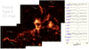 |
Fig. 1 Left panel: the positions of the background sources observed here are projected against a mosaic of cutouts of Planck Type 2 integrated CO emission: the color scale runs from 0 to 23 K-km s−1. The five sources comprising the group with small N(DNM) are noted with arrows. Right panel: the HCO+ absorption profiles in all directions, shifted vertically and scaled up in some cases. |
2.2 H I column densities
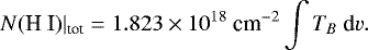
H I column densities were derived for all directions from Galactic All-Sky Survey GASS III λ21 cm H I emission spectra (Kalberla & Haud 2015). Table 1 shows total column densities N(H I) derived from the line brightness profile integral over all velocities in the optically thin limit,
Column densities of H I associated with the Chamaeleon complex, N(H I)|cham, are given in Table 2. These were derived following the methodology described by Planck Collaboration Int. XXVIII (2015) and Remy et al. (2018). GASS III H I emission profiles were decomposed into pseudo-Voigt profiles (Gaussian cores with the possibility of co-centered Lorentzian wings) and the profile integrals of all components centered within the velocity range of the Chamaeleon complex were summed, again in the optically thin limit that provided the best fit in the analysis of Planck Collaboration Int. XXVIII (2015).
2.3 DNM
Maps of the column density of dark neutral medium – the component that is not fully visible in H I or CO emission – were published for most of the sightlines by Planck Collaboration Int. XXVIII (2015). Specific values of N(DNM) along the present sightlines were extracted from that work for the present use, along with values toward J1136 and J1147 that were just outside the region considered by Planck Collaboration Int. XXVIII (2015). for their interstellar fit but still in the analysis region. All of these values are given in Table 2. N(DNM) is comparatively small in five directions and no DNM was needed along three of these: a determination of N(DMN) was made along all sightlines including those for which 0-values are given in Table 2.
2.4 CO emission
The derivation of N(DNM) by Planck Collaboration Int. XXVIII (2015) used NANTEN maps of J = 1 − 0 CO emission from Mizuno et al. (2001). The CO emission map in Fig. 1 uses the Planck Type 2 CO product which is virtually indistinguishable from the NANTEN map in a blink comparison.The rms of the Planck Type 2 CO product over the fields comprising Fig. 1 is Δ WCO = 0.45 ± 0.05 K-km s−1, leading to a detection limit comparable to that of the NANTEN maps, about 2 K-km s−1 (Mizuno et al. 2001). It should be noted that the Planck CO maps have been hashed over small regions in the immediate vicinity of several of our sightlines, presumably as the result of point-source removal, something of a Catch-22 situation for the present study.
2.5 Reddening and dust optical depth
The 6′ resolution dust-emission maps scaled to optical reddening EB−V by Schlegel et al. (1998) are cited in Tables 1 and 2. Those reddening values can be converted to Planck 353 GHz dust optical depth using the relationship established by Planck Collaboration XI (2014) between the 353 GHz dust optical depth and the EB−V values of Schlegel et al. (1998), EB−V/τ353 = (1.49 ± 0.03) × 104 mag.
Sightline and spectral line properties.
Target by target sightline gas and dust properties in descending N(DNM) order.
2.6 Conventions
Velocities presented with the spectra are taken with respect to the kinematic definition of the local standard of rest. N(H) is the column density of H-nuclei in neutral atomic and molecular form, N(H) = N(H I) + 2N(H2).
3 Molecules and dark neutral medium in the Chamaeleon complex
The use of H I, CO, Planck sub-mm dust and Fermi γ-ray emission observed on 4′ –16′ and larger angular scales to derive gas properties across the Chamaeleon complex was discussed by Planck Collaboration Int. XXVIII (2015) and further refined by Remy et al. (2018). This work adds the information gained from molecular absorption profiles observed along 13 sightlines toward point-like extragalactic mm-wave continuum sources that otherwise serve as phase calibrators for the ALMA telescope.
The angular resolution of interferometric absorption line observations is the apparent angular size of the background source in the presenceof interstellar scattering, which is milli-arcseconds at radio wavelengths: the instrumental resolution, approximately 1′′ during the observing, does not determine this. Broader-beam emission observations do more spatial averaging, but both types of observationsdo comparable sampling of the gas along the line of sight which is the more important aspect. Differences between emission and absorption line profiles generally reflect the character of the gas distribution, not the differing spatial resolution that was employed to obtain them (Clark 1965).
This work takes advantage of the fact that HCO+ absorption is more widespread than CO emission (Lucas & Liszt 1996; Liszt & Lucas 1998; Liszt & Pety 2012), presumably because N(CO) varies so sharply with N(H2) and EB−V (Burgh et al. 2007; Sonnentrucker et al. 2007; Sheffer et al. 2008) while N(HCO+)/N(H2) can be taken as constant. The net result is that HCO+ absorption is the more reliable tracer of H2 along the lines of sight observed here and even very extreme differences in angular resolution may introduce scatter, but do not introduce bias. To accommodate this, we derive and tabulate the properties of the gas along the individual sightlines (Tables 1 and 2), as we must, but the discussion is cast in terms of the average properties of two groups and the differences between them. Discussion of individual sightlines is largely left for the concluding parts of the discussion and the final figure.
3.1 General properties
General properties of the sightlines studied here are given in Table 1, with entries as explained in Sect. 2. A finding chart is presented in Fig. 1, where the locations of the continuum targets are shown against a background image of the Planck Type 2 CO map and the 5 sightlines having small column densities N(DNM) < 0.5 × 1020 cm−2 are noted. All of the HCO+ absorption profiles are shown in right panel in Fig. 1, in some cases scaled up for easier viewing: they are shown again in Fig. 2 with the NANTEN CO profiles (see Sect. 3.2).
The continuum sources sample the borders of the CO emission distribution and avoid the regions of detected CO emission, except for J1723. A recent search of the ALMA calibrator database for newly discovered strong continuum background targets in Chamaeleonwas not fruitful. Unless weaker continuum sources are used, the current survey represents the state of the art in this part of the sky.
In Table 2 the sources are reordered by descending N(DNM), and grouped according to whether N(DNM) ≳ 2× 10²⁰ H cm−2 (eight sources) or N(DNM) < 0.5 × 10²⁰ H cm−2 (five sources). The sightlines with smaller N(DNM) are called out in Fig. 1 where it is seen that they occur across the entire length of the Chamaeleon cloud complex. This is noteworthy, given the limited kinematic range of the molecular absorption in these directions, see Sect. 3.2.
The two groups have similar mean total H I column density ⟨N(H I)|tot⟩ = 13 × 1020 cm−2 averaged over all sightlines in each group, similar mean N(H I) associated with Chamaeleon ⟨N(H I)|cham⟩ = 5.6−6.6 × 1020 cm−2 and similar mean total column density per unit reddening ⟨N(H)/EB−V ⟩ ≈ 5.4−6.7 × 1021 cm−2 (mag)−1, but the group of eight DNM-rich sightlines has much larger mean reddening ⟨EB−V⟩ (0.33 vs. 0.18 mag), mean DNM column density ⟨N(DNM) ⟩ (3.3 vs. 0.14 × 1020 cm−2) and column density of H-nuclei in molecular form ⟨2N(H2)⟩ (5.6 vs. 0.83 × 1020 cm−2). Their similarity in terms of the total column density per unit reddening is only possible because of the larger contribution of H2 in the group with higher mean reddening.
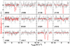 |
Fig. 2 Comparison of NANTEN CO emission (black) and ALMA HCO+ absorption (red) profiles in the directions observed. The CO emission is shown on the main-beam scale of the NANTEN telescope in Kelvins and the HCO+ absorption profiles have been scaled up by a factor three. CO was reliably detected only toward J1723 and not observed toward J1147 (not shown here). |
3.2 Kinematics and abundance
The kinematic signature of the difference between the two groups is illustrated in Fig. 3 where the mean H I profiles for each group (left panel) and their difference (right panel) are plotted along with the mean HCO+ optical depth profile, suitably scaled. The figure makes the point that the difference in H I, an increase, occurs at 2–8 km s−1 where most of the molecular gas is found. The low-velocity component of HCO+ at v ≈ 0.5 km s−1 is quite widespread, being present toward J1136, J1147, J1550 and J1723 and is present in both DNM-groups.
This point is further elaborated in Fig. 4, comparing the mean HCO+ optical depth profiles in the two groups. HCO+ absorption in the group with lower N(DNM) is of course weaker, but it also occurs only at v≲2 km s−1. As shown inFig. 1, sightlines with small N(DNM) span the breadth of the Chamaeleon complex and in principle could sample the full range of velocities, but they do not. This suggests that the higher molecular abundance and increased kinematic complexity in the higher DNM group are associated, as, for instance, when H2 production is enhanced in the presence of slow shocks associated with turbulent flows (Micic et al. 2012; Valdivia et al. 2017)
Figure 5 compares the mean optical depth profiles of HCO+, HCN and C2H. The HCN-HCO+ relationship is monotonic in the sense that the weakest and strongest components are the same in both species but the HCN/HCO+ ratio varies and is noticeably larger in the strongest component at 4 km s−1. This mimics the N(HCN)–N(HCO+) relationship that is seen along individual lines of sight where there is a rapid increase of N(HCN) at N(HCO+) ≳ 1012 cm−2 (Liszt & Lucas 2001; Ando et al. 2016; Riquelme et al. 2018; Liszt & Gerin 2018) or N(H2) ≳ 3 × 1020 cm−2. N(HCN) and N(CN) are seen to vary in fixed proportion and CN is well known to increase in abundance for N(H2) ≳ 3 × 1020 cm−2 in optical spectroscopy of the diffuse molecular gas (Sheffer et al. 2008). Although C2H absorption is faint, the C2H and HCO+ line profiles look fairly similar. C2H is known to be present in the diffuse molecular gas in quasi-constant abundance ratio relative to CH and to HCO+. The present data are consistent with the established relation between HCO+ and C2H (Lucas & Liszt 2000; Ando et al. 2016; Riquelme et al. 2018; Liszt & Gerin 2018).
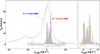 |
Fig. 3 Kinematics of the H I, separated by N(DNM). Left panel: shown separately are the mean H I profiles for the two groups of sources according to their N(DNM): H I emission in the group having more DNM is plotted as a red histogram and emission in the other group is shown as a blue line. Also shown is the mean HCO+ optical depth profile for all sources scaled upward by a factor 150. Right panel: as in left panel but the H I profile plotted in orange is the difference of the H I profiles shown in left panel. The greatest difference between the H I profiles coincides with the peak of the HCO+ optical depth. |
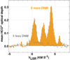 |
Fig. 4 Kinematics of the molecular gas traced by HCO+, separated byN(DNM). Shown separately are the average HCO+ optical depths of the five sources with weak NDNM (dark gray histogram) and the eight sources with stronger N(DNM) (orange bars). |
3.3 Balance among N(H2), N(DNM) and N(H I)
Overall, the hydrogen in the outskirts of the Chamaeleon complex is mainly in atomic form. In ascending order, averaged over all sightlines, ⟨N(DNM)⟩ = 2.1 × 1020 cm−2, 2N(H2) = 3.8 × 1020 cm−2 ⟨N(H I)|cham⟩ = 6.2 × 1020 cm−2 and this ordering applies to most of the sightlines individually as well. There is only one direction (J1152) where N(DNM) even slightly exceeds N(H I)|cham and only three where 2N(H2) > N(H I)|cham. The point is that the molecular component must represent a minority fraction of the total hydrogen even if all the DNM turns out to be H2. As summarized in Table 3, H2 comprises 46% of the H-nuclei in the group having more DNM, but only 13% otherwise and 36%, about one-third, in total. Overall, the molecular/atomic balance of the outlying Chamaeleon gas is very similar to that of the diffuse ISM as a whole, with estimates of the hydrogen fraction in H2 ranging from 25% to40% (Savage et al. 1977; Liszt & Lucas 2002).
Mean column densities according to sightline sample.
3.4 CO emission, observed and expected
The NANTEN CO profiles toward our targets are shown and compared with the ALMA HCO+ absorption profiles in Fig. 2, except toward J1147 that was not covered in the CO mapping. CO emission was reliably detected only toward J1723 where the CO and HCO+ lines coincide in velocity and WCO = 2.4 K-km s−1. The CO profile toward J0942 is suggestive, given the overlap with HCO+ absorption, but other equally strong and apparently spurious features are present in the CO spectrum. Weak spurious signals in consecutive channels are seen in many CO spectra. For example, toward J1312 there are three equally strong positive-going features, only one of which coincides with the HCO+ absorption, and three comparably strong negative-going features. Moreover, the HCO+ absorption toward J1312 is too weak to support a credible CO detection, as is also the case for J1152. For J1224, a weak positive-going CO feature near 0-velocity is too far removed from the HCO+ absorption to be reliable.
A null CO signal, WCO = 0, was therefore taken in all directions except J1723 in the succeeding discussion. In this regard, note that we hedged this assumption with an accepted ALMA Cycle 5 proposal to search for CO absorption so that our assumption of null detections will be tested. Perhaps more importantly, the main conclusions of this work do not stand to be affected by overlooking a few weak detections of CO emission. The corresponding amounts of molecular hydrogen are small compared to the quantity of DNM, and small compared to the amounts of H2 that was inferred from the HCO+ absorption.
The sightlines toward J1723 and J0942 have the highest molecular column density and would be expected to have the strongest CO emission. A typical global average for the conversion from N(H2) to WCO is  = 2 × 10²⁰ H2 cm−2 (K-km s−1)−1 and the right-most column of Table 2 shows the predicted CO brightness derived from N(H2) as
  = N(H2)/
 . The calculated values of
  for J1723 and J0942 from the entries in Table 2 are 2.8 and 2.0 K-km s−1, respectively (the observed value for J1723 is 2.4 K-km s−1), and there are three other cases in the higher-DNM group for which
  ≳ 1.5 K. Thus, a CO survey with a robust detection limit of 1 K-km s−1 over an approximately 8 km s−1 velocity interval (therange observed here) might detect CO in a few other sightlines in the group with higher N(DNM).
3.5 The CO-H2 conversion factor
A direct comparison of the measured WCO and inferred N(H2) toward J1723 gives N(H2)/WCO = 2.3 × 10²⁰ H2 cm−2 (K-km s−1)−1: the HCO+ abundance chosen here quite generally yields XCO ≈  in direct comparison between HCO+ absorption and CO emission in galactic disk gas (Liszt et al. 2010; Gerin & Liszt 2017). By contrast, studies like that of Planck Collaboration Int. XXVIII (2015) using dust and γ-ray or dust and X-ray (Lallement et al. 2016) measures of column density consistently find small values XCO ≲0.7 × 10²⁰ H2 cm−2 (K-km s−1)−1 when averaged over whole structures or cloud complexes. If such small values of the CO-H2 conversion factor were applied to the sightlines detected here in HCO+, the expected WCO would have been three times higher than those in the right-most column of Table 2, and most of the sightlines in the higher DNM group would have shown detectable CO emission, some with WCO ≥ 5 K-km s−1. These were not seen by the NANTEN observations at 4′ spatial resolution and also are not present in the Planck Type 2 CO map at 6′ resolution.
For this reason we use XCO =  for the weakly emitting diffuse molecular gas detected in the outskirts of Chamaeleon, while noting that smaller values apply in gas that is brighter in CO. Small regions of high CO brightness are in fact seen in the immediate vicinity of sightlines selected on the basis of their HCO+ absorption when mapped in emission at 1′ resolution with the ARO KP 12 m antenna (Liszt & Pety 2012). Moreover, the CO-H2 conversion factors N(H2)/WCO averaged over the CO hotspots observed by Liszt & Pety (2012) are smaller than
  , as is expected for brighter CO emission from diffuse molecular gas (Liszt 2017).
3.6 Molecular, missing, and CO-dark gas
As shown in Table 2, somewhat more molecular gas was detected in total than was actually required by the DNM analysis of Planck Collaboration Int. XXVIII (2015). Figure 6 illustrates for the individual sightlines the manner in which the molecular gas absorption acts to make up the gas deficit. Along the horizontal axis is the total gas measure that is globally compared with and fit to the Fermi γ ray emission and Planck dust optical depth maps to derive N(DNM), namely N(H) = N(H I)|cham + N(DNM) + 2XCOWCO with XCO =  and WCO = 0 for all sources except J1723. Along the vertical axis we show two different versions of the total column density N(H) that is directly detectable in emission and/or absorption: at top is the combination of N(H I) and H2 determined from CO emission N(H) = N(H I)|cham + 2XCOWCO while the lower panel shows N(H) represented as the combination of N(H I) with H2 determined in HCO+ absorption, N(H) = N(H I)|cham + 2W
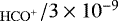 . The error bars assume ± 50% errors in WCO and N(HCO+)/N(H2).
In Fig. 6, the five sightlines with small N(DNM) are on the equality line in the upper panel when the CO emission is used, and they remain near it when H2 is derived from HCO+ because they intercept mostly atomic gas with only very weak molecular absorption. The sightline toward J1723 is near the equality line when CO is used and somewhat closer to it when N(H2) is derived from HCO+ for reasons that are discussed in Sect. 3.5. The remaining seven sightlines lie well below the equality line when N(H2) is derived from CO emission in the upper panel and bracket it when HCO+ is used.
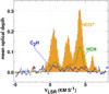 |
Fig. 5 Mean optical depth profiles for strongly polar molecules for the eight sources with N(DNM) ≳ 2 × 1020 cm−2. The HCN profile in green shows the kinematic structure that would be convolved with the HCN hyperfine splitting toreproduce the observations assuming that the hyperfine components appear in the LTE ratio 5:3:1. C2H is shown in blue. |
 |
Fig. 6 Comparison of total column density of H-nuclei N(H) derived from the DNM analysis and from observable column densities. The quantity plotted along the horizontal axis, N(H) = N(H I)|cham + N(DNM) + 2WCO |


3.7 Saturation of the λ21 cm emission
Fukui et al. (2015) and Okamoto et al. (2017) have argued that CO emission does not miss any substantial amount of molecular gas and that high optical depth and saturation of the λ21 cm H I profile can account for the DNM that is seen in analyses like that of Planck Collaboration Int. XXVIII (2015) and Remy et al. (2018). Given the pervasive molecular absorption discovered in this work, it seems difficult to support any argument that dismisses the importance of diffuse molecular gas that is missed in CO emission. However, the possible saturation of H I emission on some lines of sight is a somewhat separate issue. The DNM analysis was performed for a series of uniform gas temperatures ranging from 125 to 800 K, and it was concluded that the optically thin limit provided the best overall fit to interpret H I emission. However, it is possible that the amount of atomic gas is underestimated in localised regions.
With reference to Table 2, there is a shortfall of molecular gas, 2N(H2) < N(DNM)/2, for three of the four sources having the highest DNM values. These are the sightlines at intermediate N(H) that fall below the equality line in the lower panel of Fig. 6 and two of them have quite small values of N(H)/EB−V in Table 2. Our results show that the loss of gas due to saturation of the H I line profile is small overall because the amount of gas that would need to be added to those sightlines to bring their N(H) or N(H)/EB−V in line with the other sources is a small fraction of the total amount of gas sampled. That said, saturation of the H I profile may occur along three of the sightlines studied here, and H I absorption measurements in those directions might shed some light on this issue.
4 Summary
Using the ALMA telescope we searched for and detected 89.2 GHz HCO+ absorption in 13 directions lying toward the outskirts of the Chamaeleon cloud complex as summarized in Table 1 and illustrated on the sky in Fig. 1. The directions were selected to include the known mm-wave calibrator sources with fluxes above 125 mJy in March 2016 when the observing proposal was written, and a larger complement of strong calibrators has not been forthcoming in the intervening time. CO emission and HCO+ absorption profiles are compared in Fig. 2: CO emission had been firmly detected in only one of these directions, toward the source J1723. Weak C2H absorption was detected in eight directions and HCN emission in four directions.
As shown in Table 2, the sightlines fall into two groups having eight and five members, depending on whether the column density of dark neutral medium N(NDM) ≳ 2.0 × 1020 cm−2 or N(DNM) < 0.5 × 1020 cm−2, respectively. The two groups have similar mean total H I column density ⟨N(H I)|tot⟩ = 13 × 1020 cm−2, comparable N(H I) associated with the Chamaeleon complex ⟨N(H I)|cham⟩ = 5.6−6.6 × 1020 cm−2 (smaller in the low-DNM group) and mean total column density per unit reddening ⟨N(H)/EB−V ⟩ ≈ 5.4−6.7 × 1021 cm−2 (mag)−1. By contrast, the group of eight sightlines with more DNM has much larger mean reddening ⟨EB−V⟩ = 0.33 vs. 0.18 mag, mean DNM column density ⟨N(DNM)⟩ = 3.3 vs. 0.14 × 1020 cm−2 and mean column density of H-nuclei in molecular form ⟨2N(H2)⟩ = 5.6 vs. 0.83 × 1020 cm−2.
As shown in Figs. 3–5 and discussed in Sect. 3.2, there is a kinematic signature to the difference between the two groups, as the group with higher N(DNM) has stronger H I emission at 2 km s−1 ≲v≲ 8 km s−1, where the bulk of the molecular absorption also occurs. Molecular absorption in the group having smaller N(DNM) is confined to velocities v≲2 km s−1 even though the sightlines comprising the group span the entire breadth of the cloud complex (Fig. 1) and in principle could have sampled the full range of velocities. Molecule formation in the group with higher DNM may have been enhanced by slow shocks associated with turbulence.
On the whole, somewhat more H2 was detected in HCO+ than previously found in the DNM analysis (Table 2, Sect. 3.3) but the neutral gas in the outskirts of Chamaeleon is mostly atomic. H2 bears 46% of the H-nuclei in the group having higher N(DNM), 13% in the gas having lower N(DNM) and 36% in total. This is within the range of estimates of the molecular gas fraction in the diffuse ISM as a whole as noted in Sect. 3.3. There is no reservoir of “dark” molecular gas that went undetected as part of the inventory of dark neutral medium. Saturation of the H I profile may have caused some atomic gas to be missed along 3 of the 13 sightlines observed here (Sect. 3.6), and observationsof HI absorption might help to understand why the molecular gas column density was smaller than that of the inferred DNM in those directions. Nonetheless, DNM is overwhelmingly in the form of molecular gas overall.
Thus the situation is clear for sightlines with weak or absent CO emission in the outskirts of the Chamaeleon complex: the DNM is primarily molecular gas that was missed in CO emission and to a much lesser extent, atomic gas that might have been missed at λ21 cm. We note, however, that the present group of mm-wave bright quasars did not sample sightlines with twice-larger DNM colum densities that are present around the main Cha I and Cha II + III clouds. Probing the dense HI and diffuse H2 composition of the DNM in those directions would be valuable. DNM was also detected toward regions with high CO intensities WCO > 7 K-km s−1, which was treated as an independent component in the gamma-ray analysis of Remy et al. (2018) as it likely captures additional molecular gas in which emission saturates in the main CO isotopologue and 13CO or C18O should be used. Taking the molecular gas census in those directions would also shed important light on XCO gradients across molecular clouds.
Acknowledgements
This paper makes use of the following ALMA data: ADS/JAO.ALMA#2016.1.00714.S. ALMA is a partnership of ESO (representing its member states), NSF (USA) and NINS (Japan), together with NRC (Canada), NSC and ASIAA (Taiwan), and KASI (Republic of Korea), in cooperation with the Republic of Chile. The Joint ALMA Observatory is operated by ESO, AUI/NRAO and NAOJ. The National Radio Astronomy Observatory is a facility of the National Science Foundation operated under cooperative agreement by Associated Universities, Inc. This work was supported by the French program Physique et Chimie du Milieu Interstellaire (PCMI) funded by the Conseil National de la Recherche Scientifique (CNRS) and Centre Nationa d’Etudes Spatiales (CNES). HSL is grateful to the hospitality of the ITU-R and the Hotel Bel Esperance in Geneva during the completion of this manuscript, and the incomparable Hotel Ritz in Madrid. We thank Sarah Wood, Devaky Kunneriath and the data analysts at the North American ALMA Science Center for producing the imaging scripts for this project and sheparding it through the data reduction process. We thank the anonymous referee for comments.
References
- Ando, R., Kohno, K., Tamura, Y., et al. 2016, PASJ, 68, 6 [NASA ADS] [CrossRef] [Google Scholar]
- Burgh, E. B., France, K., & McCandliss, S. R. 2007, ApJ, 658, 446 [NASA ADS] [CrossRef] [Google Scholar]
- Clark, B. G. 1965, ApJ, 142, 1398 [NASA ADS] [CrossRef] [Google Scholar]
- Donate, E., & Magnani, L. 2017, MNRAS, 472, 3169 [NASA ADS] [CrossRef] [Google Scholar]
- Fukui, Y., Torii, K., Onishi, T., et al. 2015, ApJ, 798, 6 [NASA ADS] [CrossRef] [Google Scholar]
- Gerin, M., & Liszt, H. 2017, A&A, 600, A48 [Google Scholar]
- Grenier, I. A., Casandjian, J.-M., & Terrier, R. 2005, Science, 307, 1292 [NASA ADS] [CrossRef] [PubMed] [Google Scholar]
- Kalberla, P. M. W., & Haud, U. 2015, A&A, 578, A78 [NASA ADS] [CrossRef] [EDP Sciences] [Google Scholar]
- Lallement, R., Snowden, S., Kuntz, K. D., et al. 2016, A&A, 595, A131 [NASA ADS] [CrossRef] [EDP Sciences] [Google Scholar]
- Liszt, H. S. 2012, A&A, 538, A27 [NASA ADS] [CrossRef] [EDP Sciences] [Google Scholar]
- Liszt, H. S. 2017, ApJ, 835, 138 [NASA ADS] [CrossRef] [Google Scholar]
- Liszt, H. S., & Gerin, M. 2016, A&A, 585, A80 [Google Scholar]
- Liszt, H., & Gerin, M. 2018, A&A, 610, A49 [NASA ADS] [CrossRef] [EDP Sciences] [Google Scholar]
- Liszt, H. S., & Lucas, R. 1996, A&A, 314, 917 [NASA ADS] [Google Scholar]
- Liszt, H. S., & Lucas, R. 1998, A&A, 339, 561 [NASA ADS] [Google Scholar]
- Liszt, H., & Lucas, R. 2001, A&A, 370, 576 [NASA ADS] [CrossRef] [EDP Sciences] [Google Scholar]
- Liszt, H., & Lucas, R. 2002, A&A, 391, 693 [NASA ADS] [CrossRef] [EDP Sciences] [Google Scholar]
- Liszt, H. S., & Pety, J. 2012, A&A, 541, A58 [NASA ADS] [CrossRef] [EDP Sciences] [Google Scholar]
- Liszt, H. S., & Pety, J. 2016, ApJ, 823, 124 [NASA ADS] [CrossRef] [Google Scholar]
- Liszt, H. S., Pety, J., & Lucas, R. 2010, A&A, 518, A45 [NASA ADS] [CrossRef] [EDP Sciences] [Google Scholar]
- Lucas, R., & Liszt, H. S. 1996, A&A, 307, 237 [NASA ADS] [Google Scholar]
- Lucas, R., & Liszt, H. S. 2000, A&A, 358, 1069 [NASA ADS] [Google Scholar]
- Micic, M., Glover, S. C. O., Federrath, C., & Klessen, R. S. 2012, MNRAS, 421, 2531 [NASA ADS] [CrossRef] [Google Scholar]
- Mizuno, A., Yamaguchi, R., Tachihara, K., et al. 2001, Publ. Astron. Soc. Jpn., 53, 1071 [Google Scholar]
- Okamoto, R., Yamamoto, H., Tachihara, K., et al. 2017, ApJ, 838, 132 [NASA ADS] [CrossRef] [Google Scholar]
- Planck Collaboration XI. 2014, A&A, 571, A11 [NASA ADS] [CrossRef] [EDP Sciences] [Google Scholar]
- Planck Collaboration Int. XXVIII. 2015, A&A, 582, A31 [NASA ADS] [CrossRef] [EDP Sciences] [Google Scholar]
- Remy, Q., Grenier, I. A., Marshall, D. J., & Casandjian, J. M. 2018, A&A, 611, A51 [NASA ADS] [CrossRef] [EDP Sciences] [Google Scholar]
- Riquelme, D., Bronfman, L., Mauersberger, R., et al. 2018, A&A, 610, A43 [NASA ADS] [CrossRef] [EDP Sciences] [Google Scholar]
- Savage, B. D., Drake, J. F., Budich, W., & Bohlin, R. C. 1977, ApJ, 216, 291 [NASA ADS] [CrossRef] [Google Scholar]
- Schlegel, D. J., Finkbeiner, D. P., & Davis, M. 1998, ApJ, 500, 525 [NASA ADS] [CrossRef] [Google Scholar]
- Sheffer, Y., Rogers, M., Federman, S. R., et al. 2008, ApJ, 687, 1075 [NASA ADS] [CrossRef] [Google Scholar]
- Sonnentrucker, P., Welty, D. E., Thorburn, J. A., & York, D. G. 2007, ApJS, 168, 58 [NASA ADS] [CrossRef] [Google Scholar]
- Valdivia, V., Hennebelle, P., Godard, B., et al. 2017, ArXiv e-prints [arXiv:1711.01824] [Google Scholar]
- Weselak, T., Galazutdinov, G. A., Beletsky, Y., & Krełowski, J. 2010, MNRAS, 402, 1991 [NASA ADS] [CrossRef] [Google Scholar]
- Wolfire, M. G., Hollenbach, D., & McKee, C. F. 2010, ApJ, 716, 1191 [NASA ADS] [CrossRef] [Google Scholar]
All Tables
All Figures
|
Fig. 1 Left panel: the positions of the background sources observed here are projected against a mosaic of cutouts of Planck Type 2 integrated CO emission: the color scale runs from 0 to 23 K-km s−1. The five sources comprising the group with small N(DNM) are noted with arrows. Right panel: the HCO+ absorption profiles in all directions, shifted vertically and scaled up in some cases. |
| In the text | |
|
Fig. 2 Comparison of NANTEN CO emission (black) and ALMA HCO+ absorption (red) profiles in the directions observed. The CO emission is shown on the main-beam scale of the NANTEN telescope in Kelvins and the HCO+ absorption profiles have been scaled up by a factor three. CO was reliably detected only toward J1723 and not observed toward J1147 (not shown here). |
| In the text | |
|
Fig. 3 Kinematics of the H I, separated by N(DNM). Left panel: shown separately are the mean H I profiles for the two groups of sources according to their N(DNM): H I emission in the group having more DNM is plotted as a red histogram and emission in the other group is shown as a blue line. Also shown is the mean HCO+ optical depth profile for all sources scaled upward by a factor 150. Right panel: as in left panel but the H I profile plotted in orange is the difference of the H I profiles shown in left panel. The greatest difference between the H I profiles coincides with the peak of the HCO+ optical depth. |
| In the text | |
|
Fig. 4 Kinematics of the molecular gas traced by HCO+, separated byN(DNM). Shown separately are the average HCO+ optical depths of the five sources with weak NDNM (dark gray histogram) and the eight sources with stronger N(DNM) (orange bars). |
| In the text | |
|
Fig. 5 Mean optical depth profiles for strongly polar molecules for the eight sources with N(DNM) ≳ 2 × 1020 cm−2. The HCN profile in green shows the kinematic structure that would be convolved with the HCN hyperfine splitting toreproduce the observations assuming that the hyperfine components appear in the LTE ratio 5:3:1. C2H is shown in blue. |
| In the text | |
|
Fig. 6 Comparison of total column density of H-nuclei N(H) derived from the DNM analysis and from observable column densities. The quantity plotted along the horizontal axis, N(H) = N(H I)|cham + N(DNM) + 2WCO |
| In the text | |
Current usage metrics show cumulative count of Article Views (full-text article views including HTML views, PDF and ePub downloads, according to the available data) and Abstracts Views on Vision4Press platform.
Data correspond to usage on the plateform after 2015. The current usage metrics is available 48-96 hours after online publication and is updated daily on week days.
Initial download of the metrics may take a while.