| Issue |
A&A
Volume 675, July 2023
|
|
|---|---|---|
| Article Number | A145 | |
| Number of page(s) | 13 | |
| Section | Interstellar and circumstellar matter | |
| DOI | https://doi.org/10.1051/0004-6361/202346259 | |
| Published online | 14 July 2023 | |
The dark neutral medium is (mostly) molecular hydrogen★
1
National Radio Astronomy Observatory,
520 Edgemont Road,
Charlottesville,
VA 22903,
USA
e-mail: This email address is being protected from spambots. You need JavaScript enabled to view it.
2
LERMA, Observatoire de Paris, PSL Research University, CNRS, Sorbonne Université,
Paris,
France
e-mail: This email address is being protected from spambots. You need JavaScript enabled to view it.
Received:
27
February
2023
Accepted:
12
May
2023
Abstract
Context. More gas is sometimes inferred in molecular cloud complexes than is represented in HI or CO emission, and this is called dark neutral medium (DNM).
Aims. Our aim is to extend a study of DNM along 13 directions in the outskirts of Chamaeleon by determining the atomic or molecular character of the DNM along a larger sample of sightlines.
Methods. We acquired ALMA ground rotational state absorption profiles of HCO+ and other molecules toward 33 compact extragalactic continuum background sources seen toward the Galactic anticenter, deriving N(H2)=N(HCO+)/3 × 10−9 as before. We observed J = 1−0 CO emission with the IRAM 30m telescope in directions where HCO+ was newly detected.
Results. HCO+ absorption was detected in 28 of 33 new directions and CO emission along 19 of those 28. The five sightlines lacking detectable HCO+ have three times lower <EB–V> and <N(DNM)>. Binned in EB–V, N(H2) and N(DNM) are strongly correlated and vary by factors of 50–100 over the observed range EB–V ≈0.05–1 mag, while N(HI) varies by factors of only 2–3. On average N(DNM) and N(H2) are well matched, and detecting HCO− absorption adds little to no H2 in excess of the previously inferred DNM. There are five cases where 2N(H2) < N(DNM)/2 indicates saturation of the HI emission profile. For sightlines with WCO ≥ 1 K-km s‒1, the CO-H2 conversion factor N(H2)/WCO = 2–3 × 1020 cm‒2 /(1 K-km s‒1) is higher than is derived from studies of resolved clouds in γ-rays.
Conclusions. Our work sampled primarily atomic gas with a mean H2 fraction ≈1/3, but the DNM is almost entirely molecular. CO fulfills its role as an H2 tracer when its emission is strong, but large-scale CO surveys are not sensitive to H2 columns associated with typical values N(DNM) = 2–6 × 1020 cm‒2. Lower XCO values from γ-ray studies arise in part from different definitions and usage. Sightlines with WCO ≥ 1 K-km s‒1 represent 2/3 of the H2 detected in HCO+ and detecting 90% of the H2 would require detecting CO at levels Wco ≈ 0.2–0.3 K-km s‒1.
Key words: ISM: clouds / ISM: structure / ISM: molecules / ISM: atoms
Spectra are only available at the CDS via anonymous ftp to cdsarc.cds.unistra.fr (130.79.128.5) or via https://cdsarc.cds.unistra.fr/viz-bin/cat/J/A+A/675/A145
© The Authors 2023
 Open Access article, published by EDP Sciences, under the terms of the Creative Commons Attribution License (https://creativecommons.org/licenses/by/4.0), which permits unrestricted use, distribution, and reproduction in any medium, provided the original work is properly cited.
This article is published in open access under the Subscribe to Open model. This email address is being protected from spambots. You need JavaScript enabled to view it. to support open access publication.
1 Introduction
Between the atomic and molecular interstellar gases there is a transition that is imperfectly traced in λ121 cm HI and/or λ12.6 mm CO emission. Gas that is not well represented in one or both tracers is described as dark neutral medium (DNM; Grenier et al. 2005; Planck Collaboration Int. XXVIII. 2015; Remy et al. 2017, 2018), and the atomic or molecular character of the DNM can only be decided by appealing to other information.
In the outskirts of Chamaeleon, we used millimeter-wave HCO+ absorption to show that the DNM was almost exclusively molecular, even while the gas as a whole was mostly atomic (Liszt et al. 2018). HCO+ was detected along all 13 sampled sightlines, of which 12 lacked detectable CO emission at a level of 1.5 K-km s−1. The amount of inferred H2 was comparable to that of the DNM (confirming the amount of the detected DNM), and only for three sightlines did it seem likely that saturation of the HI emission profile could account for much of the DNM. Subsequent detections of CO absorption along six directions by Liszt et al. (2019) showed that the lack of CO emission was due to low CO column densities. The linewidth of CO absorption was shown to be smaller than that of its parent molecule HCO+, illustrating the complex chemical nature of the CO formation process in diffuse gas.
In this work, we extend the analysis of the composition of DNM to 33 sightlines in directions toward the Galactic anticenter (Remy et al. 2017, 2018) and consider the larger sample of 46 sightlines. The present study employs a relatively small number of diffuse (AV ≤ 1 mag) and translucent (AV ≤ 3 mag) sightlines where background sources are serendipitously available, and is not a revision of the earlier study, whose derived DNM column densities and other results are assumed here. Rather, we use the newly derived H2 abundances, independent of the presence of CO emission, to consider such topics as the atomic or molecular character of the DNM, the degree to which the λ21cm HI profile represents N (HI) and the influence of the CO-H2 conversion factor on the DNM determination.
Section 2 summarizes the observational material considered here and Sect. 3 compares the prior results for DNM with atomic hydrogen measured in the λ21cm emission and H2 as sampled by its proxy 89 GHz absorption of HCO+. The role of CO emission data is explored in Sect. 4 where the CO-H2 conversion factor is derived. Section 5 presents a summary, with conclusions and a discussion of later work.
2 Observations and data reduction
The methods of work were described in Liszt et al. (2018) and are not repeated in full detail here. From the existing DNM analyses of Planck Collaboration Int. XXVIII. (2015) and Remy et al. (2017, 2018) we take N(DNM) and λ21cm HI column densities N(HI) and N(HI)cl representing respectively the line profile integral integrated over all velocities and the column density that is associated with the cloud and/or kinematic features hosting the neutral gas and DNM, as derived by a decomposition that accounts for the compound nature of HI emission profiles from individual clouds.
To the exisling analyses we add ALMA observations of absorption from HCO+ and profiles oU λ12.(5 mm CO emission from the IRAM 30 m telescope, as described below.
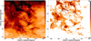 |
Fig. 1 Sky maps of the observed sightlines. Left: positions of the background sources observed here are projected against a map of EB–V from the work; of Schlegel et al. (1998). The sightlines lacking detected HCO+ absorption (largely due fo weak continuum) are indicated with smaller symbols. Right: same as left, but shown against a map of N(DNM) from Remy et al. (2017, 2018). |
2.1 Miltimeter-wave absorption
The new absorption data discussed here are spectra of HCO+ in 33 directions along Galactic anticenter sightlines toward ALMA phase calibrators as given in the Tables here and projected on sky maps in Fig. 1. As before, the HCO+ spectra were acquired with a spectral resolution of 0.205 km s−1 sampled at 0.102 km s−1 intervals without the so-called spectral averaging that bins data. We also acquired spectra of HCN, C2H, HCO, and several iso-topologs. (Counts of detections are ihown in Fig. 2, but results for species other than HCO+ will be discussed in detail in later woek. Ssattstics of the HCO+ detections are shown in Fig. A.1. Spectra in the 28 directions with detectable HCO+ absorplion are shown in Fig. B.1.
2.2 IRAM 30 m CO emission
We took frequency-switched CO emission profiles at the IRAM 30 m telescope in August 2019 toward the 28 anticenter sight-lines with detected HCO+ absorption. Thu CO spectra are shown in Fig. B.1. These CO data were taken as ftve-point maps toward the target and aisplaced by 2 HPBW (2 × 22″) in the tour cardinal directions, using a pointing pattern that was designed to detect HCO+ and HCN emission in the presence of spectral line absorption in ihe target direction. For the HCO+ emission that will be discussed in subsequent work, the HCO+ emission profile is formed by averaging spectra along the four outlying directions. For CO the present results use the average of all five pointings because contamination by absorption is not measurable given the strength of the emission and/or the continuum. The results are presented on the main beam antenna temperature scale that is native to she 30 m telescope.
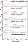 |
Fig. 2 Counts of sightlines and detected tracers binned in 0.05 intervals ot reddening, EB–V. The histogram of all sources is overlaid (dashed red) in the other panels. |
Line-of-sight properties and new results for HCO+ and CO.
2.3 Conversion from integrated HCO+ absorption to N(H2)
The suitability of HCO+ as a proxy for H2 in diffuse molecular gas was explored extensively in Liszt & Gerin (2023, hereafter Paper I). As in our earlier work, we use N(H2) = N(HCO+)/3 × 10−9 and  where
where  is the integrated HCO+ optical depth expressed in km s−1.
2.4 Reddening and dust optical depth
The 6′ resolution dust-emission maps scaled to optical reddening EB–V by Schlegel et al. (1998) are cited here. Those reddening values can be converted to Planck 353 GHz dust optical depth using the relationship established by Planck Collaboration XI (2014) between the 353 GHz dust optical depth and the EB–V values of Schlegel et al. (1998), Ев–v/τ353 = (1.49 ± 0.03) ×104 mag.
2.5 Conventions
Velocities presented with the spectra are taken with respect to the kinematic definition of the Local Standard of Rest. N(H) is the column density of H nuclei detected in neutral atomic and molecular form, N(H) = N(HI) + 2N(H2), and the molecular hydrogen and DNM fractions 2N(H2)/N(H) and N(DNM)/N(H) are respectively represented by fH2 and fDNM. The integrated absorption of the HCO+ profile in units of km s−1 is denoted by  and similarly for other species. The integrated emission of the J = 1−0 CO line is denoted by WCO with units of K-km s−1 and the CO-H2 conversion factor N(H2)/WCO is denoted by XCO. Where reference is made to a typical Galactic or standard CO-H2 conversion factor, the value N(H2)/WCO = 2 × 1020 cm−2/(1 K-km s−1) should be understood, as summarized in Table E.1 of Remy et al. (2017).
2.6 Overview
Observational results of importance to this work are given in Tables 1 and 2, and summaries of mean properties of various subsamples are presented in Table 3. Some statistics of the continuum targets and noise in the detections of HCO+ absorption are discussed in Appendix A and the CO emission and HCO+ absorption line profiles are shown in Fig. B.1 and discussed in Appendix B.
Line-of-sight properties and derived Quantities.
3 HI, DNM, and H2 sampled in HCO+ absorption
Figure 1 shows the new Galactic anticenter sightlines projected on maps of EB–V and N(DNM). The region at b < −30° is described by Remy et al. (2017) as Cetus, and that at b > −22° as Taurus-Main. California lies to the north around b = −10° and Perseus is near (l, b) = 160°,–20°. Taurus-North overlays most of the map region. The individual subregions are not discussed here owing to the sparse sampling.
Counts of sources and detected molecular tracers binned in 0.05 mag intervals of reddening are shown in Fig. 2. HCO+ is the molecular tracer detected most commonly (28 of 33 anticenter sightlines and 41 of 46 overall), followed by C2H (26 total) and HCN (21 total). The properties of molecular absorption line tracers other than HCO+ will be discussed in later work.
The Chamaeleon and Galactic anticenter subsamples have the same mode at EB–V = 0.25–0.3 mag in Fig. 2, but the anticenter subsample has a high-reddening tail at EB–V > 0.5 mag that is absent in Chamaeleon. The Galactic anticenter sample has higher mean extinction and molecular fraction. Overall (see Table 3) the anticenter sources have the following characteristics:
33% higher <EB–V> = 0.36 vs. 0.27 mag;
Same <N(HI)> = 1.3 × 1021 cm−2 and fDNM = 0.12;
80% higher <N(HI)cl> = 1.12 vs. 0.62 ×1021 cm−2;
2 times higher <2N(H2)> = 0.80 vs. 0.39 ×1020 cm−2;
65% higher

Higher fraction of detected CO, 9/33 (18/33 in the new work) vs. 1/13;
Higher incidence of nondetection of HCO+, 5/33 vs. 0/13, in some cases due to low flux, see Fig. A.1.
The DNM fraction is nearly the same in the two samples (0.12–0.13) and much smaller (0.06) in both subsamples when CO emission was detected at the level of 1 K-km s−1. The DNM fraction is also noticeably smaller when molecular gas sampled in HCO+ absorption is absent, and similarly at EB–V < 0.2 mag. The strongest variations in fDNM in Table 3 arise in selections based on the strength of CO emission and are discussed in Sect. 4.
Mean line-of-sight properties and derived quantities.
3.1 Quantitative summary results
Figure 3 shows an overview of trends in means of N(HI), N(DNM), and N(H2) using data binned in 0.05 mag intervals of reddening as in Fig. 2, plotted horizontally at the mean EB–V in every bin. The counts in each bin are shown and the bins at EB–V > 0.5 mag are occupied by only one or two sightlines. The association of DNM with molecular gas is unmistakable.
The mean HI column density varies by only a factor of 3 over a wider range EB–V = 0.09−1 mag. By contrast, means of N(NDM) and N(H2) vary by factors of 50–100. The values of <N(DNM)> and <N(H2)> are comparable and increase steadily for EB–V ≲ 0.7 mag, beyond which <N(DNM)> either fails to increase or falls: the CO emission tracer used to derive N(DNM) was used effectively to account for H nuclei in H2. The cloud-associated mean N(HI)cl declines at EB–V − 0.7 mag as H2 sequesters H nuclei. The value of <N(H2)> increases up to the bins at highest EB–V where <N(H2)> ≈ <N(HI>) ≈ 2–3 <N(HI)cl> and whole sightlines are dominated by molecular gas.
The correlation between DNM and H2 is remarkable considering the vastly different scales on which EB–V, N(HI), and N(NDM) are measured (6–20′), as contrasted with  that is derived on submilliarcsecond scales from absorption against scatter-broadened compact millimeter-wave ALMA calibrator continuum sources. The same kind of correlation of tracers observed on difterent angular scales occurs in the correlation of integrated λ21cm HI optical depth with EB–V (Liszt 2021).
When HCO+ is not detected (5/46 directions) the following characteristics are found compared to sightlines with detected HCO+:
3 times lower <EB–V> = 0.13 mag;
1.3 times higher <N(H)>/<EB–V> = 8 × 1021 cm−2 mag−1;
3.5 times lower <N(DNM)> = 8 × 1019 cm−2;
2 times lower <fDNM> = 0.07;
no DNM in 3/5 cases vs 15/46 overall.
Instead, using 3σ upper limits for N(H2) we find:
>5 times lowe+ <2N(H2)>≤ 1.5 × 1020 cm−2 and
>2.5 times lower

The ensemble of sightlines with N(DNM) < 5 × 1019 cm−2 does not differ by more than 10–20% from ovher sightlines in any mean property not involaing N(DNM). The variations in N (DNM) and N(H2) stand in great contrast with N(HI) that; increases only by a factor of 3 across the figure. The rise in N(H2) accounts for the failure of N(HS) to increase at hige ЕB-V, but this could in principle also be explained by increasing saturation of the HI emission. As noted in Planck Collaboration Int. XXVIII. (2015) and further refined by Remy et al. +2018), the global DNM analysis finds the best fit with the optically thin estimate of N(HI), implicitly leaving a bigger overall role fоr molecular gas than for saturation of the HI profile.
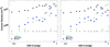 |
Fig. 3 Trends in mean N(HI), N(H2), and N(DNM) The results are binned in 0.05 mag intervals of EB–V. Left: N(HI) is calculated over the whole line profile. Rigtit: N(HI) = N(HI)cl the HI column density associated with the clouds studied here. The number of sightlines in each bin is shown in both panels. |
3.2 DNM and HI
Shown in Fig. 4 is the variation of <N(DNM)> with <N(HI)> and <N(HI)cl>. Chamaeleon differs from the Galactic anticenttr in having more extraneous atomic gas along the line of sight and smaller values of cloud-associated gas. The cloud-associated HI in Ctamaeleon is clustered at the low end of the range, even though the samples are evenly matched in the span of their total HI column density and have the same mean N(HI) in Table 3.
Sightlines lacking DNM are present at all N(HI), but N(DNM) is uniformly small along sightlines at the highest column densities N(HI) ≳ 2.3 × 1021 cm−2 where CO emission is more commonly observed. The sources with N (DNM) > 6 × 1020 cm−2 and high N(DNM)/N(HI) ratios are perhaps the most obvious candidates for hosting significant quantities of DNM in atomic form as the result of saturation of the HI profile, but only two of these actually have small contributions from N(H2). Assessing the DNM contribution arising from possible saturation of the HI profile is discussed in Sect. 3.3 where it is seen that the strongest cases of atomic DNM actually have more modest N(DNM).
3.3 DNM, EB–V, and N(H2)
As with HI, sightlines lacking DNM are present over the full range of EB–V in Fig. 5, top, but they are predominant at smaller N(H2). Sightlines with 2N(H2) ≲ 1020 cm−2 lack DNM. Along sightlines with column densities too low to host molecular gas, the atomic gas is well represented by the optically thin estimates of N(HI) used in the DNM analysis.
Care must be taken in interpreting the relationship of DNM and N(H2) in Fig. 5 because the DNM in part represents material that is missing in the CO emission tracer while some of the H2 traced by HCO+ is actually visible in CO emission. To minimize this cross-contamination, Fig. 6 shows a plot of N(DNM) vs. N(H2) fot sightlines lacking a detection of CO, using the more sensitive IRAM data for the Galactic anticenter subsample. Included are all but one (12/13) of the Chamaeleon sightlines and 60% oº those toward the anticenter.
Sightlines lacking DNM in the absence of CO emission in Fig. 6 are almost entirely confined at 2N(H2) ≲ 2× 1020 cm−2, so the detections of HCO+ ebsorpiion do not imply much additional gas along sighllines where DNM was noi found. Missing from Fig. 6 ate sightlinss with 2N(H2) ≳ 1021 cm−2 corresponding to WCO = 2.5 K-km s−1 for the Galactic CO-H2 conversion factor.
There are two or three cases in each subsample where N(DNM)/2N(H2) ≳ 2 and saturation of the λ21cm emission profile may be important. Most of these sightlines have modest values N(DNM) ≈4–5 × 1020 cm−2 and are not the sightlines with high N(DNM) that were singled out for discussion in Sect. 3.2 when comparing N(DNM) and N(HI).
There are also two or three sightlines at N(H2) > 6 × 1020 cm−2 where N(DNM)/2N/(H2) < 2. Overall <2N(H2)> = 1.3<N(DNM)> for sources lacking CO emission, so H2 accounts for DNM without adding extra “dark” gas, and the DNM is mostly molecular. As before in Chamaeleon, the DNM is large)y molecular, even if the medium overall is predominantly atomic.
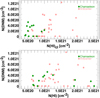 |
Fig. 4 N(DNM) plotted against to tal sightľme N(HI) (bottom) and cloud-associated atomic hydrogen N(HI)cl (top). |
4 The role of CO emission
The CO emission that was detected in previous studies used to determine N(DNM) along our sightlines was well above 1 K-km s−1 in every case (Table 2), with <WCO> = 4.9 K-km s−1 (Table 3). This is very nearly the same mean as for the sample of sightlines with WCO ≥ 1K-km s−1 observed at the IRAM 30 m, 5.5 K-km s−1 (see Table 2). Compared to the overall average, the sightlines with <WCO> ≥ 1K-km s−1 have the following characteristics:
50–100% higher <EB–V> = 0.–0.7 mag;
3–4 times higher <2N(H2)> = 2–3 × 1021 cm−2;
2 times higher

2 times lower <fDNM> = 0.06.
The 50% smaller DNM fractions <fDNм> = 0.06 along samples of sightlines with <WCO> ≥ 1K-km s−1 indicate that CO emission is doing a good job of tracing H2 in gas where the molecular fraction is high (Liszt 2017), CO emission is strong, and the cloud-associated HI fraction declines (Fig. 2). However, CO emission in general represents a small portion of the total molecular gas present along the sightlines in this work. For instance, <2N(H2)> = 7 × 1020 cm−2 along 46 sightlines, while < WCO> ≈ 5 K-km s−1 along the 6–10 sightlines where < WCO> ≥ 1K-km s−1 (Table 3). For a typical Galactic CO-H2 conversion factor, the summed molecular gas column represented in HCO+ is three to four times that inferred from the summed CO emission. Most of the molecular gas in our sample was hidden in the DNM prior to our work and is still only revealed by the HCO+ absorption, even with more sensitve CO observations. The IRAM 30m detections with < WCO> below 1 K-km s−1 comprise less than 20% of the total amount of CO emission.
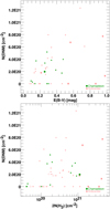 |
Fig. 5 N(DNM) plotted against EB–V (top) and 2N(H2) (bottom). Larger symbols represent sightlines where WCO ≳ 1 K-km s−1. |
4.1 The СO-H2 conversion factor
Comparison of the scaled HCO+ absorption and IRAM 30 emission measurements provides the most direct determination of the actual CO-H2 conversion factor along me lines of sight studied in this work. Figure 7 shows the trends in <N(H2)>, <WCO>, and <N(H2)>/<WCO> binned in 0.05 mag increments of EB–V as in Fig. 3. Included are the 28 Galactic anticenter sightlines whert HCO+ was detected, with WCO token at ihe 3σ upper limit for sightlines where CO emission was not detected with greater signtficance. Also included is the sightline toward J1733 in Chamaeleon where CO emission was detected. The 3σ upper limits WCO ≤ 1.5 K-km s−1 in Chamaeleon are not useful.
Figure 7 illustrates the behavior of the CO-H2 conversion factor that is tabulated for different samples in Table 3. The val-ues of <N(H2)> and <WCO> both increa^ steadily with EB–V in Fig. 7, but at different rates so that their ratio decline2 by a factor ≈7 to <N(H2)>/<WCO> = 2.5–3 × 10²⁰ H2 cm−2 (K-km s−1)−1 for EB–V ≳ 0.5 mag. Variations of similar magnitude in individual diffuse and/or translucent MBM clouds were reported by Magnani et al. (1998) and Cotten & Magnani (2013).
Mean values of N(H2)/Wсо are 2–2.5 × 10²⁰ H2 cm−2(K-km s−1)−1 for the old and new samples with <WCO> ≥ 1 K-km s−1, increasing by factors of 2–3 for the samples with IRAM 30 m detections below 1 K-km s−1 and upper limits. Also see the inset in Fig. 7 on this point.
The values of the CO-H2 conversion factor derived are comparable to those derived in extant Galactic-scale γ-ray analyses (Table E.1 in Remy et al. 2017) when WCO ≳ 1 K-km s−1, but are uniformly larger than those derived in cloud-level studies like the DNM analysis whose results are summarized in Table 2 of Remy et al. (2017). Those results ranged from 1 − 1.6 × 10²⁰ H2 cm−2 (K-km s−1)−1 for determinations based on dust and from 0.44−1.00 × 10²⁰ H2 cm−2 (K-km s−1)−1 for determinations based on γ-rays.
There is no contradiction with the larger values found in this work; whose method of studying widely separated, semirandomly placed sightlines is similar to the larger scale studies. The strongly CO-emitting (WCO > 10 K-km s−1) regions encountered in ihe cloud-level studies that have generally small values of XCO (see Fig. 13 in Remy et al. 2018) were not sampled here.
There may also be a difference arising from the operational definition of the conversion factor. The conversion factors in Table 2 in Remy et al. (2017) are those that optimize the fit of the γ-ray or dust emissivity to a total hydrogen column density that is represented schematically as N (H) = N (HI) + N(DNM) + 2N(H2) = N(HI) + N(DNM) + 2XCOWCO. After the analysis, there remains a DNM constituent whose molecular fraction is undetermined and not explicitly considered in the def-inition of the multiplier XCO; we showed that the DNM is largely molecular. By contrast, the present analysis determines N(H2) independent of CO emission and defines XCO = N(H2)/WCO. This N(H2) includes the molecular component of the DNM that we took pains to consider separately in the discussion of Fig. 6.
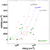 |
Fig. 6 N(DNM) plotted against N(H2) for sightlines lacking detected CO emission in the analysis of Remy et al. (2018). Shown are loci at which the number of H nuclei in H2 is 50, 100, and 200% of that in DNM. |
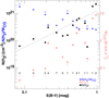 |
Fig. 7 Trends in mean N(H2) (black squares), WCO (pink; diamonds), and N(H2)/WCO (blue Wangles). The results are binned in 0.05 mag intarvalf of EB–V, as in Fig. 3. Bins in which all sightlines have only upper limits on WCO are indicated by upper and lower limits. The scale s for N(H2) cm−2 and N(H2)/WCO (cm−2 (K-km s−1)−1) are read on the left vertical axis and thaf for WCO (K-km s−1) on the right. The number of sightlines in each bin is sfown as in Fig. 3 and the count is carried separately for WCO at low EB_V. The light gray dashed line is a power-law fit |

4.2 Achievable limits and detection thresholds for CO, DNM, and H2
Sightlines in our study often had rms CO emission noise ΔWCO ≳ 1/3–1/2 K-km s−1 in the prior DNM analysis (Table 2). For a typical Galactic conversion 2N(H2)/WCO = 4 × 1020 cm−2 (K-kms)−1, the equivalent 3σ threshold detection limits on the hydrogen column are 2N(H2) = 4–6 ×1020 cm−2, above the actual values of N(DNM) along most of the sightlines we observed. By contrast, the median 3σ detection threshold from HCO+ in our work is 2N(H2) > 1.1 × 1020 cm−2 and typical N(DNM) values are N(DNM) ≳ 2 × 1020 cm−2 (Fig. 6).
The effectiveness of reducing the detection threshold of CO emission below 1 K-km s−1 can be assessed by examining the distribution of CO detections and upper limits in the IRAM 30 m CO observations. The subsamples of IRAM CO observations summarized in Table 3 show 6 detections with WCO > 1 K-km s−1, 12 detections with WCO < 1 K-km s−1, and ten upper limits at levels WCO < 0.1–0.2 K-km s−1 (see Table 1 for values of upper limits and Fig. 3 for a graphical representation of the data). HCO+ was detected along all of these sightlines, and the three subsamples respectively represent fractions 0.66, 0.26, and 0.08 of the total amount of H2.
Thus, a survey with a detection limit of 1 K-km s−1 would detect approximately two-thirds of the molecular gas along these diffuse and/or translucent lines of sight, and a much increased effort to reduce the detection limit to 0.2 K-km s−1 might find another one-fourth of the H2. Comparable reductions in the fraction of undetected H2 with increasing CO sensitivity down to rms levels ΔWCO ≈ 0.1 K-km s‒1 were achieved by Donate & Magnani (2017). Missing one-third of the H2 at the 1 K-km s−1 threshold is consistent; with the dark gas fraction derived by Wolfire et al. (2010) and Gong et al. (2018).
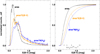 |
Fig. 8 Probability distributions of area, amount of material, and molecular hydrogen with respect to EB−V. Left: counts (probability density) scaled to the same area. Right: cumulative distribution function. N(H2) is calculated using the mean power-law fit |

4.3 The wider view
In Sect. 4.2, we note that two-thirds of the H2 was found along the sightlines with WCO > 1 K-km s−1 and that a deeper survey with a detection limit of 0.2 K-km s−1 would have found another 25% of the H2. At this point we can ask how the results of this sparse sampling are reflected in the region as a whole. We drew a hull around the observed anticenter sightlines, as shown in Fig. C.1 and derived the pixel-by-pixel statistics for the contained area, the amount of material (taken proportional to ЕB−V), and the amount of H2. For H2 we used the N(H2)-EB−V relationship  1 and the fact that; WCO ≳ 1 K-km s−1 at EB−V ≳ 0.4mag or N(H2) ≳ 4 × 1020 cm−2 in Fig 7 (see also Fig. 5 of Paper I).
Figure 8 shows the probability densities (at left) and cumulative distributions for the derived quantities. Reading values off the cumulative probability distributions at; right in Fig. 8, conditions with EB−V ≥ 0.4 mag, N(H2) ≳ 4 × 1020 cm−2 occur over one-fourth ot the tolal area containing one-half ot the total projected gas column and two-thirdt of the H2. Apparently, the sampled sightlines were representative of the region as a wbole regarding the H2 distribution.
Sampling 90% of the H2 would require detecting CO emission at EB−V ≳ 0.2 mag where N(H2) ≈2× 1020 cm−2. The sampling here is too sparse to derive an equivalent value of WCO in Fig. 7, but the broader sample in Paper I suggests WCO ≳ 0.3 K-km s−1 would be appropriate. Sightlines with EB−V < 0.32 mag or Av < 1 mag comprise two-thirds of the area, one-third of the mass, and one-fourth of the H2.
4.4 Comparison with, predictions and models
For models, the critical factors in predicting me amount of dark gas are the threshold where WCO reach es the 1 K-km s−1 brightness level and the amount; of material above the threshold. In the regime of diffuse molecular gas the integrated brightness of the J = 1-0 line is determined almost axctusively by tha CO column density, with WCO (K-km s−1) = N (CO)/1015 cm−2 for hydrogen number densities n(H) = 64–500 cm−3 (Liszt 2007, 2017; Hu et al. 2021) and kinetic temperatures appropriate to the local thermal pressure. This simple proportionality between column density and brightness persists well beyond the CO column density where the J = 1−0 transition becomes optically thick, owing to the strongly subthermal excitation (Goldreich & Kwan 1974).
Thus, the CO chemistry dominates the CO brightness and the sky map of CO emission is a map of the chemistry The observations can be reproduced by an ad hoc CO formation chemistry in which a fixed reletive abundance of HCO+ N(HCO+)/N(H2) = 3 × 10⁻⁹ thermally oecombtnes to CO if the H2 formntion and shielding of H2 and CO are treated self-consistonfly along with the heating and cooling Liszt (2017). However, networks of chemical reactions in quiescent gas may fail to form the observed quantity of HCO+ and produce too tittle CO. This causes the CO brightness to reach 1 K-km s−1 at overly large values of EB−V and N(H2) where shielding of CO by dust; and H2 make up for the deficit in the CO formation rate (e.g., Gong et al. 2018, Fig. 7; Hu et al. 2021, Fig. 9).
Models with a weak; CO formation chemistry have an innate tendency to overestimate the amount of CO-dark gas, but the actual amount of CO-dark gas depends on the distribution of material. In practise the DNM fraction seen by Remy et al. (2018) varied front 0 to 0.3 (their Fig. 8) anh the sightlines sampled here had <fDNM> = 0.10.
5 Summary
We took 89.2 GHz ALMA HCO+ absorption spectra toward 33 compart rmllimeter-wave extragalactic continuum sources seen against the Galactic anticenter (Fig. 1 and the tables above). We also observed J = 1-0 CO emission at the IRAM 30 m telescope in the 28 anticenter directions where HCO+ was detected. Inferring N(H2) from N(HCO+) using the ratio N(HCO+)/N(H2) =3 × 10⁻⁹, we combined these results with those from our earlier study of 13 directions where HCO+ absorption was detected in the outskirts of Chamaeleon. We compared the inferred N(H2) with prior determinations of the column densities of the dark neutral medium, the neutral gas of uncertain (atomic or molecular) character that had been found to be missing in HI and/or CO emission when compared with the submillimeter dust and γ-ray emissivities of large-scale molecular cloud complexes.
Binning the HI, H2, and DNM column densities in reddening, we showed in Fig. 3 that the mean DNM and molecular gas column densities were comparable and varied compatibly by factors of 50–100 over the observed range EB−V = 0.09−1 mag, while N(HI) varied by only factors of 2–3. The means of N(H2) and N(DNM) are small at low mean reddening, and increase in similar fashion up to EB−V = 0.5 mag where molecular gas begins to dominate and CO emission is strong. N(H2) continues to increase with higher reddening, but N(DNM) and the column density of cloud-associated HI fall where H2 dominates (sequestering hydrogen) and CO emission is stronger and more closely representative of N(H2).
We made detailed individual sightline-level comparisons of N(DNM) with EB-V, N(HI), and N(H2) in Figs. 4–6. Sightlines with appreciable DNM appear at all N(HI) (Fig. 4); the overall mean DNM fraction fDNM = N(DNM)/(N(HI) + 2N(H2)) = 0.12 is modest. Sightlines with appreciable DNM are lacking when EB−V ≲ 0.15 mag (Fig. 5) and when 2N(H2) ≲ 1020 cm−2 or 2N(H2) ≲ 1021 cm−2 (Fig. 6). In Fig. 6, we compared N(DNM) and N(H2) in directions lacking detected CO emission in order to eliminate the case that H2 was already represented by CO emission in the DNM analysis. This figure showed that there were 2–3 sightlines in each subsample (Chamaeleon and anticenter) or 5–6/46 overall where 2N(H2) < ≤ N(DNM)/2 and H2 accounted for the minority of the DNM. There are also a few directions at 2N(H2) ≈ 1021 cm−2 where 2N(H2) > 2N(DNM). Overall, the amounts of DNM and H2 are similar <2N(H2)> = 1.3 < N(DNM)> for the unambiguous cases lacking CO emission. The form of the DNM is overwhelmingly molecular hydrogen.
Directions with <WCO> >1 K-km s−1 have two times smaller mean DNM fractions <fDNM> = 0.06, while sightlines with <WCO> < 1 K-km s−1 have three times higher fDNM ≳ 0.17−0.19 (Table 3). The relatively few sightlines with WCO ≥ 1 K-km s−1 contain two-thirds of the H2 detected in HCO+, and detecting 90% of the H2 would require detecting CO at levels WCO ≈ 0.2−0.3 K-km s−1.
The CO-H2 conversion factor falls steadily with increasing EB−V or WCO in Fig. 7. Because the H2 is concentrated in the sightlines with WCO ≥ 1 K-km s−1, the overall mean CO-H2 conversion factors in our work are <N(H2)>/<WCO> = 2−3 × 10²⁰ H2 cm−2 for samples of sightlines with detectable CO emission. These values are comparable to previously determined large-scale Galactic averages, and are substantially higher than the global values determined by the cloud-level analyses quoted here to derive N(DNM). We ascribed these differences in part to the present sampling of widely scattered sightlines (i.e., that we did not do a cloud-level analysis) and perhaps to differences in the operational definition of the conversion factor, as discussed in Sect. 4.1.
Subsequent papers derived from the observations discussed here will focus on the physics and chemistry of the molecules observed in the course of this work, chiefly HCO+, C2H, and HCN.
Acknowledgements
The National Radio Astronomy Observatory (NRAO) is a facility of the National Science Foundation, operated by Associated Universities, Inc. This work was supported by the French program “Physique et Chimie du Milieu Interstellaire” (PCMI) funded by the Conseil National de la Recherche Scientifique (CNRS) and Centre National d’Études Spatiales (CNES). This work is based in part on observations carried out under project number 003-19 with the IRAM 30 m telescope. IRAM is supported by INSU/CNRS (France), MPG (Germany) and IGN (Spain). This paper makes use of the following ALMA data. ALMA is a partnership of ESO (representing its member states), NSF (USA) and NINS (Japan), together with NRC (Canada), NSC and ASIAA (Taiwan), and KASI (Republic of Korea), in cooperation with the Republic of Chile. The Joint ALMA Observatory is operated by ESO, AUI/NRAO and NAOJ. We thank Isabelle Grenier for providing results of the DNM analysis and we thank the anonymous referee for many helpful remarks. HSL is grateful for the hospitality of the ITU-R and the Hotel de la Cigogne in Geneva during the completion of this manuscript.
Appendix A Statistics of HCO+ detections
HCO+ absorption was not detected in five directions, all in the Galactic anticenter sample. Figure A.1 shows  plotted against its rms error
  , in essence against the strength of the continuum background since all sightlines were observed for the same length of time. The plot shows that even the noisiest sightlines miss relatively small amounts of molecular gas. The bias in the plot, whereby
  increases with
  , was to some extent built into the observing to increase the yield. That is, the source selection began with flux-limited samples that would achieve a mmimum signal-to-noise ratio on the weakest source, and added 50% additional targets at lower flux Sv and higher EB−V/SV that could be serendipitously observed without a proportionate increase in the required observing time.
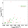 |
Fig. A.1 Integrated HCO+ optical depth |

Appendix B Spectra of HCO+ and CO
Spectra of HCO+ absorption and CO emission in the 28 directions with detected HCO+ absorption are shown in Figure B.1. The HCO+ absorption is the negative-going signal shown in red. The black histogram shows the CO emission. The frequency-switched IRAM 30m CO spectra were delivered only after folding in frequency, preventing a separation of the phases of the frequency-switching cycle using the methods of Liszt (1997). Negative-going features in the CO spectrum are artifacts; only the positive-going CO signal coincident with HCO+ absorption is interstellar.
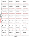 |
Fig. B.1 Spectra of HCO+ absorption (red) and CO emission (black) from the Galactic anticenter sample. For an explanation of the appearance of the frequency-switched IRAM 30m emission spectra, see Appendia B. |
Appendix C Area used to derive large-scale statistics
To derive the statistical distributions shown in Figure 8 and discussed in Section 4.4, we drew a hull around the observed sightlines as illustrated in Figure C.1 and summed over the interior pixels.
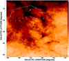 |
Fig. C.1 As in Figure 1, left, but showing the outlines of an area containing the observed sightlines used to derive large-scale properties of the anticenter region (see Section 4.3). |
References
- Cotten, D. L., & Magnani, L. 2013, MN, 436, 1152 [NASA ADS] [Google Scholar]
- Donate, E., & Magnani, L. 2017, MNRAS, 436, 1152 [Google Scholar]
- Goldreich, P., & Kwan, J. 1974, ApJ, 189, 441 [CrossRef] [Google Scholar]
- Gong, M., Ostriker, E. C., & Kim, C.-G. 2018, ApJ, 858, 16 [Google Scholar]
- Grenier, I. A., Casandjian, J.-M., & Terrier, R. 2005, Science, 307, 1292 [Google Scholar]
- Hu, C.-Y., Sternberg, A., & van Dishoeck, E. F. 2021, ApJ, 920, 44 [NASA ADS] [CrossRef] [Google Scholar]
- Liszt, H. 1997, A&AS, 124, 183 [NASA ADS] [CrossRef] [EDP Sciences] [Google Scholar]
- Liszt, H. S. 2007, A&A, 476, 291 [NASA ADS] [CrossRef] [EDP Sciences] [Google Scholar]
- Liszt, H. S. 2017, ApJ, 835, 138 [NASA ADS] [CrossRef] [Google Scholar]
- Liszt, H. 2021, ApJ, 908, 127 [NASA ADS] [CrossRef] [Google Scholar]
- Liszt, H., & Gerin, M. 2023, ApJ, 943, 172 [NASA ADS] [CrossRef] [Google Scholar]
- Liszt, H., Gerin, M., & Grenier, I. 2018, A&A, 617, A54 [NASA ADS] [CrossRef] [EDP Sciences] [Google Scholar]
- Liszt, H., Gerin, M., & Grenier, I. 2019, A&A, 627, A95 [NASA ADS] [CrossRef] [EDP Sciences] [Google Scholar]
- Magnani, L., Onello, J. S., Adams, N. G., Hartmann, D., & Thaddeus, P. 1998, ApJ, 504, 290 [NASA ADS] [CrossRef] [Google Scholar]
- Planck Collaboration XI. 2014, A&A, 571, A11 [NASA ADS] [CrossRef] [EDP Sciences] [Google Scholar]
- Planck Collaboration Int. XXVIII. 2015, A&A, 582, A31 [NASA ADS] [CrossRef] [EDP Sciences] [Google Scholar]
- Remy, Q., Grenier, I. A., Marshall, D. J., & Casandjian, J. M. 2017, A&A, 601, A78 [NASA ADS] [CrossRef] [EDP Sciences] [Google Scholar]
- Remy, Q., Grenier, I. A., Marshall, D. J., & Casandjian, J. M. 2018, A&A, 611, A51 [NASA ADS] [CrossRef] [EDP Sciences] [Google Scholar]
- Schlegel, D. J., Finkbeiner, D. P., & Davis, M. 1998, ApJ, 500, 525 [Google Scholar]
- Wolfire, M. G., Hollenbach, D., & McKee, C. F. 2010, ApJ, 716, 1191 [Google Scholar]
 at ЕB−V = 2 mag if N(H)/ЕB−V = 6−8 × 10²¹ mag−1.
All Tables
All Figures
|
Fig. 1 Sky maps of the observed sightlines. Left: positions of the background sources observed here are projected against a map of EB–V from the work; of Schlegel et al. (1998). The sightlines lacking detected HCO+ absorption (largely due fo weak continuum) are indicated with smaller symbols. Right: same as left, but shown against a map of N(DNM) from Remy et al. (2017, 2018). |
| In the text | |
|
Fig. 2 Counts of sightlines and detected tracers binned in 0.05 intervals ot reddening, EB–V. The histogram of all sources is overlaid (dashed red) in the other panels. |
| In the text | |
|
Fig. 3 Trends in mean N(HI), N(H2), and N(DNM) The results are binned in 0.05 mag intervals of EB–V. Left: N(HI) is calculated over the whole line profile. Rigtit: N(HI) = N(HI)cl the HI column density associated with the clouds studied here. The number of sightlines in each bin is shown in both panels. |
| In the text | |
|
Fig. 4 N(DNM) plotted against to tal sightľme N(HI) (bottom) and cloud-associated atomic hydrogen N(HI)cl (top). |
| In the text | |
|
Fig. 5 N(DNM) plotted against EB–V (top) and 2N(H2) (bottom). Larger symbols represent sightlines where WCO ≳ 1 K-km s−1. |
| In the text | |
|
Fig. 6 N(DNM) plotted against N(H2) for sightlines lacking detected CO emission in the analysis of Remy et al. (2018). Shown are loci at which the number of H nuclei in H2 is 50, 100, and 200% of that in DNM. |
| In the text | |
|
Fig. 7 Trends in mean N(H2) (black squares), WCO (pink; diamonds), and N(H2)/WCO (blue Wangles). The results are binned in 0.05 mag intarvalf of EB–V, as in Fig. 3. Bins in which all sightlines have only upper limits on WCO are indicated by upper and lower limits. The scale s for N(H2) cm−2 and N(H2)/WCO (cm−2 (K-km s−1)−1) are read on the left vertical axis and thaf for WCO (K-km s−1) on the right. The number of sightlines in each bin is sfown as in Fig. 3 and the count is carried separately for WCO at low EB_V. The light gray dashed line is a power-law fit |
| In the text | |
|
Fig. 8 Probability distributions of area, amount of material, and molecular hydrogen with respect to EB−V. Left: counts (probability density) scaled to the same area. Right: cumulative distribution function. N(H2) is calculated using the mean power-law fit |
| In the text | |
|
Fig. A.1 Integrated HCO+ optical depth |
| In the text | |
|
Fig. B.1 Spectra of HCO+ absorption (red) and CO emission (black) from the Galactic anticenter sample. For an explanation of the appearance of the frequency-switched IRAM 30m emission spectra, see Appendia B. |
| In the text | |
|
Fig. C.1 As in Figure 1, left, but showing the outlines of an area containing the observed sightlines used to derive large-scale properties of the anticenter region (see Section 4.3). |
| In the text | |
Current usage metrics show cumulative count of Article Views (full-text article views including HTML views, PDF and ePub downloads, according to the available data) and Abstracts Views on Vision4Press platform.
Data correspond to usage on the plateform after 2015. The current usage metrics is available 48-96 hours after online publication and is updated daily on week days.
Initial download of the metrics may take a while.