© ESO 2018

1 Introduction

PSR B0943+10 (originally named PP 0943, with PP standing for Pushchino pulsar) is one of several dozen pulsars that have been discovered in the late 1960s, during the very first few years of pulsar astronomy (Vitkevich et al. 1969). It is a relatively old (characteristic age τ ≈ 5 Myr), non-recycled pulsar, mostly known for its two stable, recurring modes of electromagnetic emission.

Once in a few hours, PSR B0943+10 switches abruptly between so-called Bright and Quiet modes (hereafter B and Q; Suleymanova & Izvekova 1984). At radio frequencies, the pulsar is a few times brighter in B mode, and its single pulses form regular drifting patterns within the on-pulse longitude window (Taylor & Huguenin 1971). With the onset of Q mode, the drift disappears, the flux density drops, and the shape of the average profile changes (Suleymanova & Izvekova 1984; Suleymanova et al. 1998). Mode transitions also affect the properties of the high-energy emission of the pulsar (Hermsen et al. 2013). In X-rays, the pulsar is ~2.4 times brighter in the radio-quiet mode, and the emission has a different spectral shape than in B mode. The X-ray emission from both modes has a pulsed thermal component that originates in a hot polar cap (Mereghetti et al. 2016).

The broadband nature of the mode-switching phenomenon may point to some global-scale magnetospheric transformation during the mode transition (Timokhin 2010). However, the exact mechanism of the mode-switching remains unclear.

Observing PSR B0943+10 with the new generation of sensitive low-frequency radio telescopes with large fractional bandwidths may provide valuable input to solving the mode-switching puzzle. At frequencies below 200 MHz, the average profile morphology starts to evolve rapidly in the B and Q modes. Within the framework of radius-to-frequency mapping theory (Cordes 1978), this means that below 200 MHz, a greater range of emission heights can be observed at once. At the same time, the pulsar is quite bright in this frequency range, so that it is possible to track the changes in the average profile shape on timescales of a few minutes and also to observe the individual pulses directly.

In our previous paper (Bilous et al. 2014; hereafter B14), we used 21 hr of LOFAR observations (mainly in the 25–80 MHz frequency range) to explore the frequency evolution in the average profile of PSR B0943+10 and to follow the gradual changes in profile shape within several mode instances. We here explore the B-mode subpulse drift in the 25–80 MHz frequency range based on the three observing sessions from B14. The subpulse drift is traditionally explained to occur through the influence of the gradient of the accelerating potential in the polar gap, which causes the fixed configuration of the emitting region to rotate slowly around the magnetic axis (“carousel model”; Ruderman & Sutherland 1975; van Leeuwen & Timokhin 2012). Thus, the drift properties are linked directly to conditions in the polar gap and provide a handle on the magnetospheric state in general.

For PSR B0943+10, the properties of drifting single pulses were also used to establish the basic magnetospheric geometry: the angles between spin and magnetic axes, and the impact angle of the observer’s line of sight (LOS). Based on the analysis of the frequency-dependent separation between B-mode average profile components and the brief presence of a 37-period modulation in the amplitudes of drifting subpulses, Deshpande & Rankin (2001; hereafter DR01) concluded that PSR B0943+10 is an almost aligned rotator. Such a geometry is hard to reconcile with the large fractional amplitude of the polar cap X-ray pulsations that were found recently (Mereghetti et al. 2016).

After a brief introduction of the observing setup in Sect. 2, in Sect. 3 we review the derivation of the geometry in DR01 and test it against LOFAR observations. We outline the data processing and drift parameterisation in Sect. 4. In Sects. 5 and 6 we present the search for subpulse periodicity in both modes, confirm the lack of periodicity in Q mode, and describe the observed properties of the drift in B mode. In Sect. 7 we attempt to constrain the number of sparks using so-called “phase tracks” (variations of immediate drift phase within the on-pulse window).

Owing to the broadband nature of our observations, we were able to detect a so-called frequency-dependent phase delay, first discovered for PSR B0809+74 by Hassall et al. (2013). In addition to variation within the on-pulse window, single pulses at different parts of the observing band have different drift phases at the same time. In Sect. 8 we show for the first time that the frequency-dependent phase delay of PSR B0943+10 has a simple quantitative geometric explanation within the carousel model. We give a short summary of our findings and conclude in Sect. 9.

2 Observations

PSR B0943+10 was observed with the low-band antennas (LBAs) of the LOFAR core stations at three epochs, with a total observing time of 15.8 hr. Raw complex voltages of two linear polarisations from each station were coherently summed, and the total intensity samples were recorded in a filterbank format. We here work with the uncalibrated total intensity signal. For the expected amounts of fractional linear and circular polarisations of PSR B0943+10 (Rankin & Suleymanova 2006), the contamination of Stokes I by the leakage from the other components of the Stokes vector is expected to be small, of the order of few percent (Noutsos et al. 2015; Kondratiev et al. 2016).

The pulsar was detected in the frequency range of 25− 80 MHz. A short summary of the observations is given in Table 1, which lists the observation ID (ObsID), the date, and pulsar modecoverage for each session. For details on the observing setup and initial data processing, we refer to B14.

3 Magnetospheric geometry of PSR B0943+10

Two essential components of magnetospheric geometry are the inclination angle, α, and the impact angle, β. In general, α is defined as the angle between the spin and magnetic axes, and β is the angle between the magnetic axis and the observer’s LOS at the moment of closest approach. In this moment, the LOS passes through the plane defined by the spin and magnetic axes, called the fiducial plane (Fig. 1).

Unfortunately, there is no uniform convention for the range of possible values of α and the sign of β in the published works (see discussion in Everett & Weisberg 2001; hereafter EW01). For example, DR01 measured α from the rotational pole that is closer to the observer and is confined to the first quadrant: 0° < α < 90°. For any α, the impact angle, β, is negative when the LOS passes polewards from the magnetic axis (inside traverse) and positive otherwise (outside traverse).

A more uniform convention was adopted by EW01; this is used in this paper as well. The geometry in EW01 is determined by the inclination angle, α, and the viewing angle, ζ, which is the angle between the spin axis and the LOS. Both α and ζ are measured clockwise from the direction of the angular momentum vector of the pulsar and can have any value between 0° and 180°. The impact angle, β, is measuredclockwise from the direction of magnetic axis and is therefore positive when ζ > α and negative otherwise.

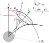Fig. 1 Sketch of basic magnetospheric geometry. The angular momentum $\overline{\text{Ω}}$ of the pulsar is directed vertically and the magnetic dipole vector $\overline{\mu }$ is inclined by the angle α. The angle between the spin axis and the LOS is the viewing angle ζ. The LOS vector stays fixed in space while the pulsar rotates around the spin axis in counter-clockwise direction. The sketch shows the moment in time when the magnetic dipole and LOS vectors lie on the same plane, corresponding to the fiducial rotational longitude, ϕ0. In this plane, the angle between an observer and the magnetic axis is β. Following EW01, α, and ζ are measured clockwise from the direction of $\overline{\text{Ω}}$, and β is measured clockwise from the direction of $\overline{\mu }$ (see text for more details). The thick black line shows an example of a dipolar field line, and the thick grey line marks the emission cone with an opening angle, ρ. Two components of the observed average profile are separated by ϕsep in rotational longitude. The dashed-line spherical triangle is shown in the inset, with PA being the measured position angle of the linearly polarised radiation, and ψ being the magnetic azimuth. We note that β, ζ, and ρ are usually plotted shifted to the common origin in the centre of the star (e.g. Lorimer & Kramer 2004; Fig. 3.4a). This transformation does not change the subsequent derivations in the text.

3.1 Derivation of geometry in DR01

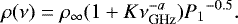
Deshpande& Rankin (2001) started their derivation by analysing the frequency dependence of the observed profile width w(ν), which can be related to the frequency-dependent opening angle of the emission cone ρ(ν) by the expression (Gil et al. 1984) $$\cos \rho =\cos \alpha \cos (\alpha +\beta )+\sin \alpha \sin (\alpha +\beta )\cos (w/2).$$(1)

The authors take the functional form of the ρ(ν) dependence from the study of Mitra & Deshpande (1999; hereafter MD99), who analysed the multi-frequency width measurements of 37 pulsars with both cone and core components. For these pulsars, α was taken from the limiting width of the core component, w = 2.45°/($\sqrt{P_1}\sin \alpha$) and β from the maximum value of the PA gradient (Lyne & Manchester 1988; Rankin 1990, 1993b). It is worth mentioning that for some of the pulsars in the sample of MD99, different α and β were later obtained by EW01. MD99 fitted their multi-frequency ρ(ν) measurements with the relation: $$\rho (\nu )={\rho }_{\infty }(1+K{\nu }_{\text{GHz}}^{-a})P_1{}^{-0.5}.$$(2)

Here ρ_∞ is the opening angle of the emission cone at infinite radio frequency, and $P_1{}^{-0.5}$ is the inverse square root of the pulsar period (see also Rankin 1993a).

Deshpande & Rankin (2001) defined w as the distance between the outer half-maximum points on the average profile. The authors performed least-squares fits of Eqs. (1) and (2) to seven measurements of w at frequencies between 25 and 111 MHz. They used a set of trial α, β, and a, while leaving K fixed at the best-fit value from MD99, K = 0.066. The opening angle of the emission cone at infinite frequency was set by ${\rho }_{1\text{\hspace{0.05em}GHz}}={\rho }_{\infty }\times 1.066\times P_1{}^{-0.5}$ at the values for the inner and outer cone from Rankin (1993a), namely at ρ_{1 GHz} = 4.3° and 5.7°, respectively (B14 erroneously quoted these values as coming from MD99).

The fit resulted in three solution branches: “inside traverse”, “outside traverse”, and “pole-in-cone” models. For all three models the choice of ρ_{1 GHz} had little influence on the quality of the fit. Quoting DR01, “it appears that models with any reasonable 1-GHz ρ values will behave similarly”.

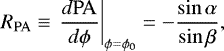
The best-fit α and β from all three models can then be used to calculate the swing of the linearly polarised radiation position angle under the assumptions of the rotating vector model (RVM; Radhakrishnan & Cooke 1969), and the results can be compared to the observations. For this comparison, DR01 used the absolute value of the maximum gradient of the PA angle |R_PA| = |sinα∕sinβ| (see also Rankin (1993a) and the discussion in EW01). The inside and outside traverse models resulted in |R_PA| similar to the observed value, whereas the pole-in-cone model yielded an incompatible R_PA and thus was rejected.

The inside traverse model gave the following pairs of geometry angles: α_DR = 15.39° and β_DR = −5.69° for the outer-cone ρ_{1 GHz}, and α_DR = 11.58°, β_DR = −4.29° for the inner-cone ρ_{1 GHz}. The values for the outside traverse model were similar, but with positive β. The outside and inside traverse geometries prescribed different behaviour of the magnetic azimuth ψ(ϕ), since for the small ϕ − ϕ₀, it is proportional to sin(α + β) (see Sect. 7). The rate of magnetic azimuth change can be externally constrained if the number of sparks in the carousel N is known: the change in magnetic azimuth between the adjacent subpulses detected within the same pulse period should be equal to 360°∕N. DR01 deduced N = 20 from the 37P₁ modulation of the drifting subpulse amplitudes, observed in a subset of their pulse stacks (see Sect. 6.2). The inside traverse model predicts the correct number of sparks, whereas the outside traverse model predicts approximately eight sparks and therefore is rejected.

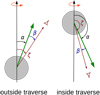Fig. 2 Pulsar orientation angles for the two branches of our geometry fit. The pulsar rotates counter-clockwise, and the spin axis is shown by the vertical arrow. The shorter green arrows show the magnetic axis, and the brown arrows show the LOS. The branches are labelled outside traverse and inside traverse to match the notation of DR01; inside/outside refers to the relative position of the LOS direction with respect to the smaller angle between the spin and magnetic axes. We follow the definition of (α, β) in EW01, which is different from the one used by DR01. The conversion between the two notations is given in Table 2.

3.2 Geometry fit with LOFAR observations

We repeatedthis analysis based on 45 ϕ_sep values from four observing sessions in B14. These measurements were obtained by fitting two Gaussian components to the session-integrated average B-mode profiles at frequencies between 26 and 80 MHz. We chose to fit the separation between components, not the full width at half-maximum (FWHM), since the latter is affected by smearing at the low edge of the band (below 40 MHz) due to the incoherent de-dispersion (B14). At the same time, using ϕ_sep facilitates comparison with MD99, who performed their analysis for the radius of the maximum intensity inside the cone.

Similarly to DR01, we find two solution branches: one with α <90°, and another with α > 90°, corresponding to outside and inside traverses in their notation (see Fig. 2). Since we did not detect a 37P₁ modulation of the subpulse amplitudes (Sect. 6.2), we chose not to reject the outside traverse branch.

The outside and inside traverse models constrain β quite well, but give comparable values of χ² for a wide range of α. To constrain α further, we used R_PA = −2.9 ± 0.5°/° from Suleymanova et al. (1998). This range reflects the likely uncertainty on R_PA: other works also give R_PA = −2.7°/° (DR01) and − 3.0°/° (Backus et al. 2010). Similarly to EW01, we used the following expression for the R_PA: $$R_{\text{PA}}\equiv {\frac{d\text{PA}}{d\varphi }|}_{\varphi ={\varphi }_0}=-\frac{\sin \alpha }{\sin \beta },$$(3)

which fixes a widespread error regarding the direction of position angle growth on the sky: the classical expression for the PA swing in RVM was derived assuming that the PA increases clockwise on the sky, whereas the actually measured PA increases counter-clockwise on the sky (following the standard astronomical convention, e.g. van Straten et al. 2010).

In contrast do DR01, the outside traverse resulted in a better fit in our case, with a reduced χ² of about 2.7, while the inside traverse gave about 3.9. The fit was consistently better at steeper values of R_PA, but we did not try to minimise the χ² by varying R_PA. We note that fitting for K in Eq. (2) and with better measurements of PA may result in better χ², but exploring this is beyond the scope of the current analysis. It is also possible that the errors on ϕ_sep, set by the two-Gaussian fit in B14, are underestimated.

Similarly to DR01, we found that the quality of fit was the same for the inner and outer cone values of ρ_{1 GHz}. Considering that ρ_{1 GHz} has a direct influence on the derived (α, β) and given the absence of any additional information about the opening angle of the PSR B0943+10 emission beam (although the steep spectral evolution of the separation between profile components may give preference to the outer cone, with ρ_{1 GHz} close to 5.7°; Rankin 1993a), it seems reasonable to explore the possible range of (α, β) values under the assumption that ρ_{1 GHz} lies somewhere within the values found in MD99. Thus, we repeated the fit for a set of trial 2° < ρ_{1 GHz} < 8°, loosely corresponding to the 2.9° < ρ_{1 GHz} < 7.3° span of calculated ρ_{1 GHz} in the sample of pulsars in MD99 for P₁ ≈ 1.1 s. The (α, β) for different ρ_{1 GHz} are plotted in Fig. 3. The errors on (α, β) are set by the uncertainties in R_PA. The power-law index in Eq. (2), a, was 0.45 for outside traverse and 0.33 for inside traverse. As a rule of thumb, for any chosen ρ_{1 GHz}, β ≈ρ_{1 GHz}, in line with DR01’s statement that the LOS grazes the edge of the emission cone at frequencies ≳ 1 GHz. The inclination angle α for the outside traverse, and 180°−α for the inside traverse, increases with ρ_{1 GHz} approximately as 3ρ_{1 GHz}.

Deshpande & Rankin (2001) give the numerical values of the geometry angles only for the inside traverse solution branch. For the inner and outer cone ρ_{1 GHz}, their (α, β) are within our range of possible values (Fig. 3).

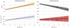Fig. 3 Pulsar orientation angles based on the analysis of frequency-dependent component separation and the PA sweep rate versus the assumed value of the emission cone opening angle at 1 GHz, ρ1 GHz. The black lines show α(ρ1 GHz) and β(ρ1 GHz) for RPA = −2.9°/°. Shaded regions mark a ± 0.5°/° uncertainty in RPA, where the lower edge corresponds to a lower absolute value of RPA. The stars mark the DR01 geometry solutions corresponding to the inner and outer cone ρ1 GHz (white and black, respectively). The angles were converted into the EW01 notation according to Table 2.

4 Single-pulse analysis: data processing and drift parameterisation

For the single-pulse analysis, the signal was de-dispersed, integrated in frequency within several sub-bands, and folded synchronously with the topocentric pulsar period to form frequency-resolved “pulse stacks”, s(ϕ, t), 2D arrays of the uncalibrated total intensity as a function of rotational longitude and time. In this notation, time is assumed to be constant within each rotational period: t = [pulse number] × P₁.

The signal within each pulse period and sub-band was normalised by subtracting the mean and dividing by the standard deviation of noise in the off-pulse window. Pulse stacks from the B and Q modes were analysed separately, for which the few-second region around the mode transition was removed. The mode transitions were identified visually through abrupt (within a few rotation periods) start or cessation of the subpulse drifting patterns.

In this paper we adopt the somewhat simplified version of the drift parameterisation from the work of Edwards & Stappers (2003; hereafter ES03). The authors treated pulse stacks as the sum of steady and drifting components (the steady component can also depend on ϕ and t, but in aperiodic fashion). The drifting component can be expressed as $$s_{\text{drift}}(\varphi ,t)~A(\varphi )\times \text{Re}\left[\exp \left(2\pi it/{\widehat{P}}_3+i\theta (\varphi )\right)\right].$$(4)

Here, A(ϕ) is the variation in the pulse amplitudes within the on-pulse window, on average described by the shape of the average profile, ${\widehat{P}}_3$ is the observed modulation period along the lines of constant ϕ, and θ(ϕ) is the so-called “drift phase”. The drift phase accrues 360° between twoadjacent subpulses that are recorded within the same pulse period. The observed longitudinal spacing between such subpulses is called ${\widehat{P}}_2$: $${\widehat{P}}_2=P_1{\left[\frac{\text{d}\theta }{\text{d}\varphi }\right]}^{-1}.$$(5)

A cartoon with drifting subpulses together with their respective ${\widehat{P}}_2$ and ${\widehat{P}}_3$ is shown in Fig. 4.

As noted by ES03, for the parameterisation given by Eq. (4), the apparent direction of drift (i.e. whether pulses seem to march towards the leading or trailing edges of the profile) depends not on the sign of ${\widehat{P}}_3$ or dθ∕dϕ, but on whether they both have the same sign (in general, the sign of dθ∕dϕ is constant throughout the on-pulse window, although a few exceptions are known; see Champion et al. 2005; Weltevrede et al. 2006; Szary & van Leeuwen 2017). If the sign of dθ∕dϕ (and thus ${\widehat{P}}_2$) matches the sign of ${\widehat{P}}_3$, subpulses will appear earlier with each successive period thus, drifting towards the leading edge of the average profile. In the case of opposite signs, subpulses will appear to be drifting to the trailing edge of the average profile. To avoid confusion, ES03 assumed that dθ∕dϕ is always positive and let the sense of drift be determined by the sign of ${\widehat{P}}_3$.

The properties of subpulse drift are traditionally assessed through so-called longitude-resolved fluctuation spectra (LRF spectra; see Backer (1970; DR01). An LRF spectrum consists of 1D Fourier transforms of the pulse stacks, computed over the lines of constant rotational longitude. If the time-dependent subpulse modulation is present at the spin phase ϕ, the Fourier transform ofs(t) for that ϕ will have two peaks at Fourier frequencies of ${\nu }_t=\pm 1/{\widehat{P}}_3$. Since the peaks are present in both the positive and the negative half of the Fourier spectrum, it is not possible to determine the sign of ${\widehat{P}}_3$ from the power spectrum alone. However, the direction of the drift can be retrieved from the complex-valued Fourier spectrum by examining the evolution of the complex phase of the transform with the longitude. If S(ϕ, ν_t) is the longitude-resolved Fourier transform of s(t), then from Eq. (5) it follows that $$\begin{array}{l}\text{Arg}\left[S(\varphi ,{\nu }_t=1/{\widehat{P}}_3)\right]~\theta (\varphi ),\\ \text{Arg}\left[S(\varphi ,{\nu }_t=-1/{\widehat{P}}_3)\right]~-\theta (\varphi ).\end{array}$$(6)

Since dArg[S]∕dϕ > 0 by definition, selecting the peak with the observed positive phase gradient will fix the sign of ${\widehat{P}}_3$ (ES03).

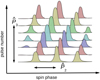Fig. 4 Example of a drifting subpulse sequence. ${\widehat{P}}_2$ corresponds to the observed longitudinal spacing between subpulses, and ${\widehat{P}}_3$ is the amount of time between subpulses that appear at the same longitude. Here, ${\widehat{P}}_3$ is equal to the integer number of the rotation periods, but this is not necessarily true in general.

5 Searching for subpulse modulation in Q mode

Normally, LRF spectra of the Q-mode pulse stacks do not exhibit any prominent peaks, indicating that the subpulses arrive predominantly chaotically within the on-pulse longitude window (Fig. 5, left; see also DR01; Rankin et al. 2003; Rankin & Suleymanova 2006). However, possible weak, intermittent, or narrowband periodicities have not been ruled out completely. Deshpande & Rankin (2001), having examined a 170-pulse sequence right after a B-to-Q transition at 430 MHz, found a weak (from a visual inspection of their Fig. 13, the LRF spectra averaged within the on-pulsewindow had a signal-to-noise ratio (S/N) of about five), but distinct feature at the frequency of 0.77 cycles/P₁. This result was not confirmed by a larger sample of five observations at 40 and 103 MHz (Rankin et al. 2003). Rankin & Suleymanova (2006) reported that the LRF spectra from a 30-min-long sequence of the Q-mode pulses right before the Q-to-B transition in one of their three 327-MHz observations had a feature at ν_t = 0.0275 ± 0.001 cycles/P₁, which is similar to the B-mode carousel circulation frequency.

Our observations contained 4.2 hr of Q-mode pulse sequences and five mode transitions, forming a good dataset to search for any potential subpulse drift in the Q mode. First, we searched for intermittent and possibly narrowband periodicities. We analysed pulse stacks from three central ≈15-MHz sub-bands (central frequencies of 39, 54, and 70 MHz). In these sub-bands, the Q-mode signal was strong enough to form a discernible average profile over the course of one session. We divided the pulse stacks into 512-pulse blocks and computed LRF spectra on each block separately. In order to reduce potential smearing of the spectral features by the slow variation of the pulse intensities (for example, at 50 MHz, the pulsar signal scintillates with a characteristic timescale of 4 min, or 240 pulsar periods, see Fig. 1 and Appendix B of B14), we subtracted a running 32-period on-pulse mean from the pulse sequences. None of the obtained LRF spectra (integrated in longitude within the on-pulse window) had features with an S∕N > 5.2. The features with an S∕N > 4 appeared tobe randomly scattered in Fourier frequency, and none of them fell within the 0.026–0.029 cycles/P₁ interval, corresponding to the range of observed carousel circulation frequencies for the B-mode pulse sequences.

In order to increase our sensitivity to broadband periodicities that are stable in time, we summed the pulse stacks from different sub-bands, re-computed LRF spectra on 512-pulse blocks, and added the spectra, forming one average LRF spectrum per an observing session. None of the these spectra had features with an S∕N > 3.8. We therefore conclude that we were unable to find any periodicities in the available Q-mode observations.

6 Subpulse modulation in B mode

6.1 Overall properties

The remarkable drift of the PSR B0943+10 subpulses (Fig. 5, right) was noted soon after the pulsar was discovered (Taylor & Huguenin 1971) and has been extensively studied since then (see, e.g. the most recent work of Backus et al. 2011, and references therein). Normally, the LRF spectra of B-mode pulse stacks present a strong feature at ν_t ≈ ± 0.46 cycles/P₁. The observed value of $|1/{\widehat{P}}_3|$ depends on the time since B-mode onset: right after Q-to-B transition, $|1/{\widehat{P}}_3|\approx 0.455$ cycles/P₁ and then it slowly relaxes to ≈ 0.47 cycles/P₁ in approximately exponential fashion (Rankin & Suleymanova 2006; Backus et al. 2011). ${\widehat{P}}_3$ is considered to be independent of observing frequency, although Rankin et al. (2003) noted small discrepancies in $1/{\widehat{P}}_3$ measured simultaneously at 40 and 103 MHz. In their work, $1/{\widehat{P}}_3$ refers to the interpolated centroid of the spectral feature, and the error comes from the formal uncertainty of centroid estimation. The discrepancies were of the order of 0.001 cycles/P₁ or a few assumed uncertainties.

In order to investigate the subpulse periodicity in our B-mode observations, we computed LRF spectra on 512-pulse blocks, divided into five sub-bands in radio frequency. Only three central sub-bands (at 39, 54, and 70 MHz) had a sufficiently high S/N to discern a subpulse periodicity in each block. The LRF spectra had peaks close to ≈ ± 0.46 cycles/P₁ in the on-pulse window. Examination of dθ∕dϕ from the positive and negative parts of the complex-valued Fourier spectrum (Eq. (6)) revealed that the phase gradient is positive for the peak at ν_t < 0. Thus, ${\widehat{P}}_3<0$ and subpulses ostensibly drift to the trailing edge of the profile (see also Sect. 8). The true sense of drift may be different due to aliasing, see the discussion in Sect. 7.

Some of our LRF spectra exhibited simple narrow peaks, similar to those presented in DR01 or Rankin et al. (2003). However, the majority of the LRF spectra appeared to have complex-shaped features with two or multiple peaks. Thus, we did not try to estimate the exact $1/{\widehat{P}}_3$ by fitting centroids to spectral features, as was done by Rankin et al. (2003). Instead, we simply compared the positions of peaks between sub-bands. We found that for all 512-pulse blocks, the peaks in different subbands fell at the same ν_t bins, indicating that the instantaneous $1/{\widehat{P}}_3$ is stable across the LBA frequency range at least to within our spectral resolution of 0.004 cycles/P₁. For the subsequent analysis, we integrated the signal in the whole band to increase the S/N and re-computed the LRF spectra in the whole band.

The upper panel of Fig. 6 shows the near-peak portion of these on-pulse-integrated LRF spectra for all of the 512-pulse blocks for the three observing sessions. This panel also shows a part of the Q-mode LRF spectra (integrated within the respective Q-mode on-pulse window). To highlight the secular evolution of ${\widehat{P}}_3$, the sessions were aligned by Q-to-B transitions. Our observations confirm the previously established secular evolution of $1/{\widehat{P}}_3$ (Rankin et al. 2003; Rankin & Suleymanova 2006; Backus et al. 2011). However, it is obvious that the spectra exhibit a variety of structures. Figure 6 (lower panels) shows the ν_t < 0 region for a pair of LRF spectra featuring two qualitative shapes of LRF features: multiple peaks (A), and a single peak (B). Previously published works acknowledged this behaviour, although no special attention has been paid to it. Suleymanova & Rankin (2009) mention two discrete jumps in the feature by 0.007 cycles/P₁ within a 700-pulse long sequence of pulses right after a Q-to-B transition. Rosen & Clemens (2008) report additional peaks of lower S/N on the sequence from Suleymanova et al. (1998), separated by about 0.003 cycles/P₁. Rankin & Suleymanova (2006) also report a few double peaks in the LRF spectra, separated by 0.007 cycles/P₁. In panel A in Fig. 6, the characteristic separation between peaks is about 4 bins, or 0.0078 cycles/P₁. This agrees with the spread of 1∕P₃ points in Fig. 3 of Backus et al. (2011; also computed based on 512-pulse sequences) and is equivalent to the spread of carousel circulation times in Rankin et al. (2003), obtained from 256-pulse LRF spectra. The multiple peaks in LRF spectra are present throughout all our B modes.

As was pointed out by Rosen & Clemens (2008), observing two values of ${\widehat{P}}_3$ simultaneously would serve as a strong corroboration to the non-radial surface oscillation model of drifting subpulses. Unfortunately, our ability to resolve the true temporal simultaneity is limited by the frequency resolution of the discrete Fourier transform, which is inversely proportional to the length of the pulse sequence. Nevertheless, we recomputed LRF spectra using the 256-pulse sequences and compared each pair with the corresponding 512-pulse LRF spectrum. For all 512-pulse LRF spectra with two distinct peaks, only one peak at a time was found in the 256-pulse subsets (see Fig. 7, left), indicating that ${\widehat{P}}_3$ can change on a timescale as short as 256P₁.

Multiple peaks in LRF spectra may partly be attributed to phase jumps, caused by momentary shifts in spark positions. As noted by Halpern et al. (2017), a sudden large (of the order of π) jump in phase of a single-frequency periodic signal can result in an apparent frequency splitting of its power spectrum, with the two new peaks straddling the frequency of the absent primary peak. We have searched forsuch frequency splitting in our observations by comparing the LRF spectra from 512- and 256-pulse sequences. In some cases we found that the pairs of 256-pulse LRF spectra have distinct peaks at the same ν_t, which did not coincide with the peak of the 512-pulse LRF spectrum (Fig. 7, right), although we did not detect a symmetric splitting corresponding to a single phase jump. A simple simulation of a sinusoidal signal with a number of various phase jumpsshowed that adding more jumps to the signal can result in uneven amplitudes of the split peaks, with one of the peaks absorbing most of the power.

Although the true drift frequency may vary on short timescales or be obscured by phase jumps, there is little doubt in its gradual evolution throughout the B mode (Rankin & Suleymanova 2006). We compared the mode-long evolution of $P_1/{\widehat{P}}_3$ from our observations to the most recent similar study of Backus et al. (2011), who observed two partial B modes with the GMRT at 325 MHz. They obtained the following expression for the ${\widehat{P}}_3$ evolution: $$-P_1/{\widehat{P}}_3=0.471-0.022\times \exp (-t/73),$$(7)

where t is the time in minutes from the onset of the B mode. As noted by the authors, the functional form of the expression is completely arbitrary, and the main purpose of the fit was to gauge the characteristic time of the parameter evolution in the B mode. Equation (7) is consistent with our measurements as well (Fig. 8), indicating that the general evolution of ${\widehat{P}}_3$ with time from the mode start does not change noticeably between 40 and 325 MHz and on a timescale of a few years, which separates our observations from those of Backus et al. (2011).

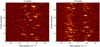Fig. 5 Example of pulse sequences in the Q and B modes from the observing session L102418. Only the on-pulse longitude region is shown. In the B mode the apparent drift period $\left|{\widehat{P}}_3\right|$ is similar to two rotation periods, which results in the distinct even-odd modulation of the subpulses (see Sect. 6 for the discussion of the ${\widehat{P}}_3$ sign). If $\left|{\widehat{P}}_3\right|$ were exactly 2P1, drifting subpulses would appear at the same longitudes during every other rotation period. Because $\left|{\widehat{P}}_3\right|$ is slightly larger than 2P1, however, thesubpulses appear to be slowly shifting towards the leading edge of the average profile, with an apparent cycle of about 10P1.

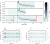Fig. 6 Topplot: stack of LRF power spectra, integrated within the on-pulse window. On the X-axis, each column corresponds to the LRF spectrum computed from 512-pulse (≈9 min) pulse stacks. Only the Fourier frequencies around the B-mode feature are shown. The S/N ratio is shown with colour. Similarly to B14, observations are aligned by the Q-to-B transition. Vertical solid lines mark B-to-Q transitions, and dashed lines show the Q-to-B transitions. The observed ${\widehat{P}}_3$ slowly evolves with time since the B-mode onset and also exhibits strong random fluctuation around the general trend. Bottom row: two examples of individual LRF spectra showing different types of P3 behaviour: multiple peaks (A) and a single peak (B). The average profiles for the corresponding pulse sequences are plotted in the side panel. Two solid vertical lines mark the supposed position of the sidelobes (for the highest S/N peak in A), calculated for the 20-spark carousel from DR01. The dotted line shows the first-degree alias of the second harmonic frequency of the highest S/N peak, and the dashed line marks the frequency of the supposed 37P1 modulation from Asgekar & Deshpande (2001).

6.2 Search for periodic amplitude modulation in drifting subpulses

Periodic amplitude modulation of drifting subpulses, reported in the work of DR01, was proven to be a vital argument for constraining several important system parameters: the number of sparks in the carousel, the degree of aliasing, and the orientation of the LOS vector with respect to magnetic and spin axes. According to DR01, this tertiary modulation manifested itself in the form of symmetric sidelobes in the LRF spectrum, 0.0268 cycles/P₁ away from the primary feature at 0.4645 cycles/P₁. These sidelobes, interpreted as an indicator of the persistent pattern in subpulse brightness, were detected only in a small, 256-pulse fraction of one 430-MHz B-mode observation.

Following ES03, the period of the tertiary modulation, P₄, can be expressed through ${\widehat{P}}_3$, together with the integer number of sparks, N, and the degree of aliasing, n, in the following way: 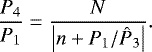$$\frac{P_4}{P_1}=\frac{N}{\left|n+P_1/{\widehat{P}}_3\right|}.$$(8)

In the work of DR01, N = 20 and n = −1, satisfying Eq. (8) for 1∕P₄ = 0.0268 cycles/P₁ and $1/{\widehat{P}}_3=0.4645$ cycles/P₁.

ES03 also noted that other solutions to Eq. (8) exist, with |n| > 1, for example n = 2 and N = 92, or n = −3 and N = 132. However, for the α and β derived using the DR01 method (Sect. 3), such solutions do not agree with the observed slope of the drift phase tracks, dθ∕dϕ = 34°/° (DR01, see also Sect. 7). The same reasoning can be used to reject a periodic spark brightness pattern, for example, sparks being brighter in the opposite quadrants of magnetic azimuth. In this case, N obtained through Eq. (8) should have been multiplied by the number of the brightness pattern repetitions.

Rosen & Clemens (2008) argued that the sidelobes may be due to the stochastic variations in the amplitudes alone. They analysed the same observation as in DR01 and found that sidelobes are present in the LRF spectrum, but are absent from the harmonic-resolved fluctuation (HRF) spectrum of the same 256-pulse sequence. An HRF spectrum, a different manner of presenting a Fourier transform of drifting subpulses, is a stack of 1∕P₁ sections of the Fourier transform taken on the entire 1D pulse sequence (see DR01). The authors performed Monte Carlo simulations of sidelobe significance by shuffling the pulse amplitudes in the sequence. The simulations showed that the chance probability of two peaks with the S/N seen in the LRF spectrum is quite low (lower than 1%), but the probability of the modulation appearing in LRF and being masked by noise in HRF spectrum is equally low.

Further confirmation of sidelobes came from Asgekar & Deshpande (2001) and Backus et al. (2010). Asgekar & Deshpande (2001) observed PSR B0943+10 with the Gauribidanur Telescope for two sessions, each ≳1000 s long. The observations were conducted at 35 MHz, with a 1 MHz bandwidth. In one of the sessions, the authors detected a peak at 0.027 cycles/P₁ (corresponding to the carousel circulation time in DR01), but without sidelobes around the primary feature. This low-frequency peak has about the same amplitude as the primary feature and appears in both LRF and HRF spectra. However, the spectrum is more noisy at frequencies below 0.1 cycles/P₁ and another peak also lies at the even lower frequency of about 0.01 cycles/P₁, which was not addressed by the authors. No low-frequency features were detected in the other session.

Backus et al. (2010) analysed 18 h of Arecibo B-mode observations at frequencies of 327 and 430 MHz and found two more instances of tertiary modulation, again in the form of sidelobes around the primary feature. In one sequence, the sidelobes were quite weak, with a visually estimated S∕N of about 3. The other sequence had more distinct sidelobes that were asymmetric in amplitude. Unfortunately, the published LRF spectra do not allow inspecting the ϕ-resolved distribution of power in the sidelobes. The authors state that modulation is rare, appearing in 5% of the time span of the observations, and that they did not detect sidelobes corresponding to any other possible values of P₄.

For the LOFAR observations, none of our LRF spectra (both in individual sub-bands and band-integrated) exhibited sidelobes corresponding to the 20-fold modulation of carousel sparks. We did not detect sidelobes for N = 20, nor for any other N between 5 and 40 (we note that this separation is much larger than the primary feature jitter in the previous section, see Fig. 6). No obvious modulation features at low Fourier frequencies were found, although in some cases, we detected occasional peaks below 0.013 cycles/P₁ or the power was uniformly rising at lower frequencies in a red-noise-like manner.

Our dataset comprises 11.6 h of B-mode observations, which makes it 1.5 times smaller than the dataset of Backus et al. (2010), which had two instances of tertiary modulation. Thus, it is possible that we did not detect the modulation solely because of its rarity. In addition, so far, the Gauribidanur and Arecibo detections of tertiary periodicity both came from relatively narrow-band observations that probed a small range of emission heights. In our observations the signal is collected from a greater range of heights, which means that if any persistent brightness pattern is frequency dependent, it might be smoothed out.

An independent confirmation of the tertiary amplitude modulation would be very important not only for constraining the system geometry and the parameters of the carousel, but also for distinguishing between the carousel and surface oscillation models of drifting subpulses (Rosen & Clemens 2008). The prospects of further investigations in this direction are quite good: recent observations of PSR B0943+10, conducted within the project of studying the simultaneous X-ray/radio mode-switching resulted in a large amount of radio data at low and high radio frequencies, surpassing all previous works (including this one) by a factor of several (Mereghetti et al. 2016). However, given the apparent absence of tertiary modulation in our observations and the concerns expressed in Rosen & Clemens (2008), we decided for now to abandon the tertiary modulation constraint and treat both n and N as free parameters.

As was noted by the referee, subtracting the running 32-period on-pulse mean may suppress possible amplitude modulation due to the ≈37-period carousel rotation. Thus, we repeated the analysis in Sect. 5 and 6 without subtracting the running mean, which yielded essentially the same results.

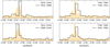Fig. 7 On-pulse averaged LRF spectra for two 512-pulse sequences (light colour, filled) together with the LRF spectra computed for the first and last 256 pulses of each pulse sequence (black, empty). Only the Fourier frequencies around the B-modefeature are shown. The pulse numbers in the legend are counted from the closest Q-to-B transition. Left: example of an LRF spectrum with two peaks that are resolved into a single peak that changes its position with time. All double features with clearly separated peaks were resolved in this way. Right: example of an LRF spectrum for a 512-pulse sequence that shows the peak offset from the peaks in the LRF spectra of the subsequences. This behaviour might be explained by phase jumps within the pulse sequence.

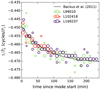Fig. 8 Primary feature of the LRF spectra from Fig. 6 for the three B-mode intervals with observed Q-to-B transitions. If the LRF spectrum had several peaks, all of them were plotted. The size of the marker corresponds to the peak S/N. The fit of Eq. (7) from Backus et al. (2011) is overplotted, which was based on two partial B-modes observed at 325 MHz.

Fig. 9 Unwrapped phase tracks, θ(ϕ) from Eq. (6) (black dots) at the Fourier frequencies corresponding to the $P_1/{\widehat{P}}_3$ peaks intwo LRF spectra with relatively strong (left) and weak (right) drifting features. The θ(ϕ) from the longitude region around the peaks of the average profile (larger markers) were used to fit the number of sparks in the carousel according to Eq. (9). Black lines mark an example of such fit performed with the standard set of geometry/aliasing parameters (see text for details), and the bottom panels show the residuals together with the fitted θ(ϕ) uncertainty. The orange line depicts the longitudinal separation between subpulses, ${\widehat{P}}_2(\varphi )$, computedby differentiating the fit line (Eq. (5)). The orange error bar at ϕ = 0 marks the ${\widehat{P}}_2$ uncertainty derived from the uncertainty in fitted N. The average profile of the pulse sequence is shown with shades of grey. For convenience, since ${\widehat{P}}_2$ is measured in degrees, the top axis shows the spin longitude ϕ in the same units.

7 Phase tracks in B mode

The complex argument θ(ϕ) in Eq. (6) can provide additional information about the subpulse drift. An example of this θ(ϕ) dependence (often called the “phase track” in the literature) is shown in Fig. 9. The θ(ϕ) accrues 360° over $\delta \varphi ={\widehat{P}}_2$, the longitudinal separation between two adjacent subpulses in the same pulse period. For PSR B0943+10, ${\widehat{P}}_2$ is close to the width of the whole on-pulse window (see also DR01 and Backus et al. 2011), meaning that only one or two supbulses are detected per P₁. This can be directly confirmed by visual inspection of the B-mode pulse sequence in Fig. 5 (right). The flattening of the phase tracks far from the fiducial longitude indicates that the longitudinal separation between subpulses is somewhat larger (by about 40%) at the edges of the on-pulse window. In the carousel model, this ϕ-dependent subpulse separation is attributed to the curvature of the line traced by the LOS vector.

As wasdemonstrated by ES03, for the carousel consisting of N uniformly spaced sparks, θ(ϕ) is given by theformula $$\theta (\varphi )=-N\psi \text{\hspace{0.17em}sgn\hspace{0.17em}}\beta +(\varphi -{\varphi }_0)\left(n+\frac{P_1}{{\widehat{P}}_3}\right)+{\theta }_0.$$(9)

Here, the first term reflects the relationship between the change in magnetic azimuth (δψ = 360°/N) and the corresponding change in drift phase (δθ = 360°) for the two adjacent sparks in a non-rotating carousel. Magnetic azimuth ψ is expressed through rotational longitude as 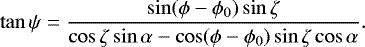$$\tan \psi =\frac{\sin (\varphi -{\varphi }_0)\sin \zeta }{\cos \zeta \sin \alpha -\cos (\varphi -{\varphi }_0)\sin \zeta \cos \alpha }.$$(10)

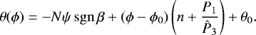
For the small ϕ, α, and ζ, this equation reduces to ψ ≈ ζϕ∕(−β). In the notation of ES03, dθ∕dϕ is always positive, thus a factor of −sgn β appears in the first term of Eq. (9). The last two terms in Eq. (9) account for the carousel rotation around the magnetic axis and positions of sparks with respect to the fiducial longitude ϕ₀.

At the fiducial longitude, ${\widehat{P}}_2$ is expressed as $${\widehat{P}}_2({\varphi }_0)=P_1{\left[N\text{sgn\hspace{0.17em}}\beta \frac{\sin \zeta }{\sin \beta }+\left(n+\frac{P_1}{{\widehat{P}}_3}\right)\right]}^{-1}.$$(11)

Although Eq. (9) provides a specific mathematical prescription for θ(ϕ), using this equation directly for constraining N and θ₀ is difficult because of the number of unknowns it contains – on the right-hand side, only ${\widehat{P}}_3$ is measureddirectly. In the rest of this section we investigate how the best-fit N depends on the chosen values for the other parameters in Eq. (9), namely the degree of aliasing n, geometry angles, and the fiducial longitude ϕ₀. We also explore the evolution of N with radio frequency and the time since the B-mode start. For the latter we chose, with some degree of arbitrariness, a “standard” set of geometry/aliasing parameters: ρ_{1 GHz} = 4.5°, R_PA = −2.9°/°, and outside traverse, n = 0.

We limited the θ(ϕ) fit to the part of the on-pulse window around the average profile peaks: 4° < |ϕ − ϕ_mid| < 12°, where ϕ_mid is the midpoint between the two Gaussians fitted to the profile components (B14). The fit was performed with a Markov chain Monte Carlo (MCMC) algorithm¹. The measured θ(ϕ) was modelled as a normally distributed random variable, with the mean set by Eq. (9) and the fitted variance (same for all points within a single phase track) representing the unknown measurement error. All fitted parameters had uniform priors, and the quality of fit was verified by comparing model predictions to the observed θ(ϕ). The quoted errors on the fitted parameters represent 16th and 84th percentiles of their respective posterior distribution.

Although a carousel model in its simplest form prescribes an integer number of sparks, in our fit we chose not to constrain N to an integer number. As we show below, for any moderate degree of aliasing, a minor (with respect to their uncertainties) tweak in the geometry angles can always be used to bring N to an integer. Also, Backus et al. (2011) speculated about a possible flickering between configurations with a different number of integer sparks, which would produce seemingly non-integer N.

7.1 Dependence on the choice of fiducial longitude ϕ₀

The rotational longitude ϕ enters Eqs. (9) and (10) in the form of ϕ− ϕ₀, where ϕ₀ is the fiducial longitude, corresponding to the moment of time when the LOS passes closest to the magnetic axis (Fig. 1). Since the illumination of the emission cone can be uneven or patchy, it may be difficult to determine the location of the fiducial longitude based on the shape of the total intensity profile at a single frequency. Linearly polarised emission can provide some clues to the location of ϕ₀: if the PA curve has an S-shape, as prescribed by the RVM, then, neglecting relativistic corrections, the fiducial longitude should lie at the inflection point of the curve (Radhakrishnan & Cooke 1969). Unfortunately, PSR B0943+10’s PA has a seemingly linear dependence on ϕ without an obvious inflection point (Suleymanova et al. 1998; Rankin & Suleymanova 2006; Rosen & Clemens 2008).

The location of ϕ₀ at 430 MHz has been constrained by DR01 and Rankin & Suleymanova (2006) with the help of the cartographic analysis (i.e. mapping individual pulses to the sparks in the carousel). The authors showed that at the onset of a B mode, ϕ₀ is located between two closely spaced components of comparable amplitudes. As a mode ages, the relative amplitude of the trailing component diminishes and the profile acquires an asymmetric shape, with ϕ₀ lying close to the trailing half-peak longitude.

Below 100 MHz, the amplitude of the second component exhibits a similar evolution with mode age, but the components are farther apart from each other and have little overlap, making it easier to decompose the average profile into Gaussian components. As was shown by B14, the midpoint between profile components follows the ν⁻² dispersion law at least between 30 and 80 MHz. This implies that the position of the midpoint is frequency independent and is thus well suited for the role of ϕ₀. However, quite surprisingly, it has been discovered that this frequency-independent midpoint gradually shifts towards later spin phase, accruing an offset of δϕ ≈ 4 × 10⁻³ by the end of a mode instance, and supposedly re-setting its position at the next Q-to-B transition (B14, Suleymanova & Rodin 2014). The reason for this delay is currently unclear and may involve, among others, changing the illumination pattern in the emission cone or a change in emission altitude (see the discussion in B14 and Suleymanova & Rodin 2014).

According to Eq. (9), the shape of phase tracks should be symmetric with respect to ϕ₀, thus the phase tracks of sufficient length and quality could, in principle, provide an alternative way to measure ϕ₀ and thereby offer an insight on the origin of the profile delay. For example, a changing illumination pattern should not affect the position of the symmetry point, while changing the emission height should result in shifting ϕ₀.

We have fitted all phase tracks from all sessions with two assumptions: (1) ϕ₀ stays constant throughout B mode, fixed at its position at the midpoint between components at the beginning of the mode, and (2) that it follows the midpoint obtained by the two-Gaussian fit from B14. These two assumptions resulted in equally good fits with an insignificant difference inN (Fig. 10). Thus, we can conclude that the shape of the phase tracks did not constrain the location of ϕ₀. Further improvements can be achieved with more sensitive observations and perhaps moving to the lower frequencies, which would expand the size of the on-pulse window.

7.2 Dependence of the number of sparks on aliasing and geometry

The fitted number of sparks, N, depends on the assumed geometry and the degree of aliasing, n. In order to investigate this dependence, we fitted Eq. (9) to θ(ϕ) from a 512-pulse block with a strong narrow drifting feature in the LRF spectrum using the set of trial geometry angles and assumed n. Since the number of sparks may change throughout the mode (Sect. 7.3), we label this single-block estimate of N the “reference number of sparks”, N₀.

For thefit, we used the geometry solutions given by the three trial values of R_PA and 13 equally spaced trial values of ρ_{1 GHz}, 2° ≤ ρ_{1 GHz} ≤ 8°. In addition, we varied the aliasing order between − 2 and 2. The fits showed that N₀ was most sensitive to the assumed R_PA, then to the degree of aliasing, and only then on the assumed ρ_{1 GHz} (Fig. 11). Outside traverse geometries generally yielded approximately twice smaller N₀ than the inside traverse ones. For the standard geometry/aliasing set of parameters, N₀ = 8.9 and 17.6 for the inside and outside traverse, respectively.

Interestingly, for the inside traverse geometry with R_PA = −2.7°/° and n = 1, as determined by DR01, our fit yields N₀ ≈ 19, which is similar to their N = 20. Thus, our results are in agreement with DR01, although abandoning the tertiary modulation constraint expands the range of possible N₀ values.

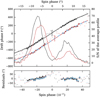Fig. 10 Phase tracks for the beginning (black) and the end (red) of the same B mode (observation L99010), with an artificial vertical offset added. The average profiles of the corresponding pulse sequences are plotted in the background with matching colours. The serifs mark the midpoint between profile components (see text for details). Lines show the fit with standard geometry/aliasing parameters. Solid lines correspond to the fit with fiducial longitude ϕ0 matching the midpoint between profile components. The light blue dashed line shows the fit to the late-mode phase track with ϕ0 fixed at the position of the midpoint between components at the onset of the B mode. Both constant and moving ϕ0 yield the same quality fits and an almost identical number of sparks N, and the change in ϕ0 is absorbed by fitted θ0.

7.3 Evolution of N and ${\widehat{P}}_2$ throughout B mode

As was discussed in Sect. 7.2, the number of sparks, N, depends on the specific values of aliasing/geometry parameters used for the fitting. The relative variation in spark number, N∕N₀ − 1, however, does not depend on the exact values of the fitting parameters. Figure 12 (left) shows N∕N₀ − 1 for every distinct peak on the LRF spectra in each of the 512-pulse blocks. The number of sparks at any moment under different aliasing/geometry assumptions can be recovered by combining N∕N₀ − 1 with N₀ from Fig. 11.

The fitted values of N jitter throughout a B mode with a characteristic magnitude of δN∕N₀ ≲ 0.02. This relative difference can be attributed to varying the integer number of sparks only if N₀ is large: N₀ = 1∕δN ≳ 1∕0.02 = 50. This can be achieved only by assuming a very high degree of aliasing. However, any conclusions here should be drawn with caution, since the nature of the drift frequency jitter (or splitting, within a single pulse block) is unclear and θ(ϕ) can be contaminated by phase jumps or phase modulation.

Apart from this erratic behaviour, N∕N₀ increases by ≈0.02 on a timescale of mode duration for the first two observations (L99010 and L102418). Correspondingly, ${\widehat{P}}_2$ for the first two sessions decreases byabout 0.2° (Fig. 12, right).

It is interesting to compare these results with those obtained by Backus et al. (2011). The authors computed HRF spectra on an unfolded time series and examined the dependence of modulation intensity on the harmonic number for the primary modulation feature. ${\widehat{P}}_2$ was calculated from the harmonic number corresponding to the peak of the modulation intensity, 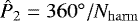${\widehat{P}}_2={360}^{°}/N_{\text{harm}}$. The ${\widehat{P}}_2$ obtained was about 11° at the beginning of the B mode and slowly decreased to about 10° in a seemingly exponential manner. The authors did not give the measurement error, but the points in their plot are scattered by about 0.5°. The authorsconsidered the on-pulse window to be small enough to neglect the longitudinal variation of ${\widehat{P}}_2$.

For the later stages of a B mode, our fit suggests a larger ${\widehat{P}}_2$, of about 10.6°, even for the lowest possible value of ${\widehat{P}}_2$ at the fiducial longitude. The values of ${\widehat{P}}_2$ in our fit depend on R_PA, with ${\widehat{P}}_2$ for R_PA = −2.4°/° being larger by 0.2° and smaller by the same amount for R_PA = −3.4°/°. Even if we obtain ${\widehat{P}}_2$ using exactly the same geometry as in DR01, it is still larger than in Backus et al. (2011), and the reasons for this are currently unclear.

In our observations, the gradual variation of ${\widehat{P}}_2$ throughout the B mode is about five times smaller than reported by Backus et al. (2011). A possible explanation for this would be the following: Backus et al. (2011) investigated HRF spectra, thus effectively probing ${\widehat{P}}_2$ at all longitudes within the on-pulse window. The size of the on-pulse window at their frequencies is ≈ 10°, and ${\widehat{P}}_2$ changes by about 1° between the centre of the window and its edges (Fig. 9). The relative contribution of ${\widehat{P}}_2(\varphi )$ at each longitude may be substantially influenced by the average intensity of emission at that longitude. At the radio frequency of Backus et al. (2011; 325 MHz), the intensity of the emission at the longitudes of trailing component undergoes substantial changes throughout the B mode: at the mode onset, the trailing component is approximately of the same height as the leading component, and at the end of the B mode, the amplitude of the trailing component is only about 20% of the leading component amplitude (Rankin & Suleymanova 2006). Thus, at the beginning of the B mode, the longitude window of the trailing component, where 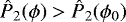${\widehat{P}}_2(\varphi )>{\widehat{P}}_2({\varphi }_0)$, is illuminated better than at the end of the mode, and this might cause observed increase in the derived ${\widehat{P}}_2$. The authors investigated the influence of profile shape evolution on the measured ${\widehat{P}}_2$. However, they explicitly simulated the intrinsic ${\widehat{P}}_2$ being constant within the on-pulse window.

The observed small changes in ${\widehat{P}}_2$ may be due to the evolution of the linear polarisation. According to Suleymanova et al. (1998) and Rankin & Suleymanova (2006), at frequencies of 100–300 MHz, the linearly polarised emission in both profile components consists of two orthogonal modes of unequal strength. It has been shown that these two polarisation modes correspond to two sets of sparks in the carousel, shifted in azimuth with respect to each other (DR01). Moreover, observations at 64 and 327 MHz revealed that the fractional linear polarisation at the peak of the leading component evolves substantially throughout B mode (Suleymanova & Rankin 2009), perhaps indicating the change in the relative strength of the polarisation modes. If the relative intensity of the two sets of sparks changes at LBA frequencies, it can add a time-dependent bias to the phase tracks, which may result in the observed variation in ${\widehat{P}}_2$. Another pulsar, for which the incoherent superposition of the two orthogonal polarisation modes led to biased measurements of ${\widehat{P}}_2$ is PSR B0809+74 (Rankin et al. 2005; Rankin & Rosen 2014).

Fig. 11 Reference number of sparks, N0, under different assumptions of the geometry angles and the degree of aliasing, n. N0 was obtained by fitting Eq. (9) to a single pulse stack with high S/N in session L99010. The left and right panels show N0 for the outside and inside traverse geometry branches. For each of the three values of RPA, namely − 3.4, − 2.9, and − 2.4°/°, a set of trial ρ1 GHz between 2° and 8° was used. For clarity, the points for different ρ0 are plotted with the horizontal offset proportional to ρ0 − 4.5°. Although the carousel model prescribes the integer number of sparks, N0 was not fixed to an integer value during the fit.

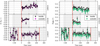Fig. 12 Left: relative change in the number of sparks for every distinct peak in each of the 512-pulse LRF spectra. The fit was performed with the standard set of aliasing/geometry parameters, for the inside (black dots) and outside (purple dots) traverse geometries. The “reference” number of sparks, N0, was taken from Fig. 11. Right: ${\widehat{P}}_2$ at the fiducial longitude, ϕ0, from Eq. (11) for inside (black dots) and outside (green dots) traverse geometries.

7.4 Number of sparks versus radio frequency

We fitted N and θ₀ to three 16-MHz subbands in the middle of the LBA band, where the S/N was highest (at 38.2, 53.8, and 69.4 MHz). The fit was performed with the standard geometry/aliasing parameters. For all pulse blocks and every pair of frequencies, |N(ν₁) − N(ν₂)| divided by the the quadrature sum of the corresponding uncertainties was lower than 3. However, there is a slight tendency for the lowest frequency to yield a higher value of N (Fig. 13, left).

A frequency-dependent number of sparks would be hard to explain with the carousel model, but a deeper investigation is needed to confirm or refute this tendency: for example with calibrated polarisation to resolve the orthogonal modes and with better sensitivity at frequencies below 40 MHz.

8 ${\widehat{P}}_3$ folds in B mode

In the schematic depiction of drifting subpulses in Fig. 4, the individual drift tracks are clearly visible because of the relatively large ${\widehat{P}}_3$ and the uniformly high S/N of the individual pulses. For PSR B0943+10, ${\widehat{P}}_3$ is comparable to P₁ and the amplitudes of the pulses can vary substantially, preventing the shape of the drift tracks from being evident in the pulse stacks alone (Fig. 5). In order to uncover the shape of the drift tracks, it is customary to fold the pulse stacks modulo ${\widehat{P}}_3$, assigning each period in the pulse stack s(ϕ, t) a “drift phase”: $$\text{Θ}=\frac{t{P}_1}{{\widehat{P}}_3}\times {360}^{°},$$(12)

where t is an integer pulse number, the same as in Eq. (4). Such folds are called “modfolds” or “driftbands” in the literature (Backus et al. 2011; Hassall et al. 2013).

At higher radio frequencies, the PSR B0943+10 modfolds consist of a single drift track spanning the entire on-pulse window (350 MHz, DR01; Backus et al. 2011). Around 100 MHz, the drift track is still continuous, but wraps twice per ${\widehat{P}}_3$ (DR01). Finally, at the lowest radio frequencies, two separate drift tracks are visible in the longitude regions of two distinct profile components (35 MHz; Asgekar & Deshpande 2001).

Figure 14 shows an example of the modfold for a single pulse stack, folded with the corresponding ${\widehat{P}}_3<0$ from Sect. 6. Unlike DR01, we did not subtract any “aperiodically fluctuating baseline“ from the modfolds, and for most of the pulse stacks, the drift tracks had a well-defined shape with little baseline signal between them. In a few cases, however, when folding the pulse stacks with multiple peaks in the LRF spectrum, the drift tracks appeared to be blurred. We note that the drift tracks in Fig. 14 are tilted to the right (pulses drift towards the trailing edge of on-pulse window), whereas in the literature the drift tracks are tilted to the left (pulses drift towards the leading edge). This discrepancy stems from difference in the period, P₃, used for folding – after DR01, all modfolds in the literature were performed with P₃ defined by the relation $$\frac{P_1}{P_3}=n+\frac{P_1}{{\widehat{P}}_3},$$(13)

where the degree of aliasing was taken to be n = 1. Drift tracks look exactly the same for any |n|, but for all n ≤ 0 the tracks are tilted to the right and for all n > 0 they are tilted to the left.

The white circles in Fig. 14 mark the centres of the drift tracks obtained from fitting 2D tilted Gaussians. We label the coordinates of the track centres (ϕ_C, Θ_C), adding L for the leading component and T for the trailing component when needed. Both ϕ_C and Θ_C appear to evolve with radio frequency, approaching each other at higher ν. This creates the apparent diagonal movement of the drift tracks, which continues beyond the LBA band; around 100 MHz, the drift tracks fuse at the inner corners and continue to merge, eventually forming a single drift track at 350 MHz. For the modfolds folded with n > 0, the direction of vertical movement is reversed for both drift tracks. The ϕ_C, obviously, corresponds to the position of the average profile components, and the decreasing |ϕ_C −ϕ₀| reflects the merging components at higher frequencies. The longitude spacing between driftband centres does not correspond to ${\widehat{P}}_2$, as the intensity within driftbands is set by the shape of the average profile.

A similar frequency-dependent Θ was found by Hassall et al. (2013) in the modfolfds of PSR B0809+74. Unlike PSR B0943+10, the Θ_LC for the pulsar B0809+74 was frequency independent and the Θ_TC was moving towards Θ_LC with increasing ν. The same behaviour was exhibited by ϕ_C: the position of the leading component was frequency independent while the trailing component was moving towards it with increasing radio frequency. Hassall et al. (2013) did not give an explanation to the observed Θ_C behaviour. However, Rankin & Rosen (2014) later suggested that it might be explained by the frequency-dependent phase delay of the rotating carousel with respect to the LOS.

Below we show that for PSR B0943+10, the observed Θ_C (ν) can be quantitatively explained within the carousel model. Without loss of generality, we consider a simplified model with simultaneous observations at only two radio frequencies, ν_hi > ν_lo. For simplicity, we assume that during the chosen traverse, the LOS cuts through the spark centres at ν_lo. At ν_hi, the same LOS sweep will miss the spark centres, causing the offset between drift tracks at different frequencies. Figure 15 shows a cartoon model of this effect for the inside traverse geometry and n = 0 modfolds. For the inside traverse geometry solution, the pulsar rotates clockwise (Fig. 2), thus the LOS sweeps from left to right on the image. Folding pulse stacks with P₃, determined by n ≤ 0 (Eq. (13)) implies that from the observer’s point of view, the carousel rotates clockwise (pulses drift towards the trailing edge of profile). Altogether, this means that at ν_hi LOS will cut through the leading part of the spark for the leading component and that the carousel will need extra time to rotate to bring the spark centre to the LOS (Fig. 15). In the modfold plots, time increases upwards, thus |Θ_LC(ν_hi)| > |Θ_LC(ν_lo)| and |Θ_LC(ν_hi)| < |Θ_LC(ν_lo)|. Folding pulse stacks with P₃, determined by n ≤ 0, reverses the assumed direction of the carousel rotation and the direction of the Θ_C shift, exactly as observed. Finally, the same reasoning applies for the outside traverse geometry solution.

Quantitatively, the drift-phase delay between two frequencies can be expressed as $$\begin{array}{lll}{\text{Θ}}_{\text{C}}({\nu }_{\text{lo}})-{\text{Θ}}_{\text{C}}({\nu }_{\text{hi}})\hfill & =\hfill & -N\text{\hspace{0.17em}sgn\hspace{0.17em}}\beta \times [{\psi }_{\text{C}}({\nu }_{\text{lo}})-{\psi }_{\text{C}}({\nu }_{\text{hi}})]\hfill \\ \hfill & \hfill & +[{\varphi }_{\text{C}}({\nu }_{\text{lo}})-{\varphi }_{\text{C}}({\nu }_{\text{hi}})]\times \frac{P_1}{P_3}.\hfill \end{array}$$(14)

Here the first term represents the scaled difference in magnetic azimuth angles calculated with Eq. (10) at ϕ_C (ν_hi) and ϕ_C (ν_lo). The second term accounts for the carousel rotation during the time it takes the LOS to travel between ϕ_C (ν_hi) and ϕ_C (ν_lo).

Bilous et al. (2014) have shown that within the LBA band, ϕ_C can be approximated with the following relation: $${\varphi }_{\text{TC/LC}}(\nu )={\varphi }_0\pm {69}^{°}.84\times {\left[\frac{\nu }{1\text{\hspace{0.17em}MHz}}\right]}^{-0.567}.$$(15)

Extrapolating this relation to infinite frequency yields ϕ_C(ν = ∞) = ϕ₀ for both profile components. This can be used to rewrite Eq. (8) with respect to ν_hi = ∞: $${\text{Θ}}_{\text{C}}(\nu )=-N\text{\hspace{0.17em}sgn\hspace{0.17em}}\beta \times \psi ({\varphi }_{\text{C}})+({\varphi }_{\text{C}}-{\varphi }_0)\frac{P_1}{P_3}+{\text{Θ}}_0,$$(16)

where Θ₀ = Θ_C(ν = ∞).

Figure 16 shows such Θ_C(ν) calculated for the standard geometry/aliasing parameters, for the reference number of sparks, N₀, and ϕ_C from Eq. (15). The phase at the fiducial longitude Θ₀ is set to 0 in this figure. Measurements of Θ_C from the Gaussian fit to drift tracks are overplotted for all phase tracks from the observing session L99010 for which the S/N of the drifting feature in the LRF spectra was higher than six (modfolds from the other two sessions exhibited the same Θ_C (ν) dependence). The modfolds were folded with P₃ determined by the corresponding distinct ${\widehat{P}}_3$ from the peaks on the LRF spectra and n = 0. Since each individual modfold was produced with sightly different ${\widehat{P}}_3$, the fiducial longitude phase Θ₀ is essentially random, and thus should be subtracted from Θ_C. To do this, we investigated 0.5(Θ_LC + Θ_TC) for the drift tracks for which the amplitudes of fitted 2D Gaussians had an S∕N > 7. For most of these cases, this mean value of Θ_C did not have a dependence on ν, thus we took it as Θ₀. Since we set the point of symmetry manually, the fixed and moving ϕ₀ hypotheses from Sect. 7.1 will both result in an identical Θ_C behaviour.

The agreement between the measurements and the prediction from the rotating carousel model is very good, although the scatter of points is larger than the formal fit errors. Several factors may contribute to the additional scatter: N may slightly vary throughout the B mode (Fig. 6), or the shape of the driftbands may deviate from simple Gaussian due to uncertainties in ${\widehat{P}}_3$, the small number of Θ bins (18), and the small number of pulses (~15) that are averaged in a single Θ bin.

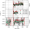Fig. 13 Relative change in the number of sparks for the three frequencies within the LBA band with respect to the reference number of sparks N0 from Fig. 11. The fit at the lowest frequency yields slightly but consistently larger N.

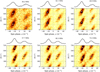Fig. 14 Example of a 512-pulse stack folded modulo ${\widehat{P}}_3$ for six radio frequencies within the LBA band. The modfold is repeated twice along the Y -axis to mitigate wrapping, and the corresponding average profile is plotted on top. White circles mark the centres of driftbands obtained from fitting 2D tilted Gaussians. As the radio frequency increases, the driftbands move towards each other both in ϕ (reflecting the behaviour of the average profile components) and in Θ.

9 Summary and conclusions

PSR B0943+10, with its two discrete metastable emission modes and the slow variation of the emission properties in (at least) one of the modes, provides a great opportunity to investigate the non-stationary magnetospheric configurations and to untangle the complex interplay between various physical processes in a pulsar magnetosphere. However, with many new facts that come to light as a result of improved observational capabilities in X-rays and at the lowest radio frequencies, it becomes increasingly important to keep track of the assumptions made to interpret previous observations.

The very basic question of the PSR B0943+10 geometry is still not answered fully. In Sect. 3 we have successfully reproduced the original geometry derivation from DR01 using the broadband LOFAR observations at 25–80 MHz. DR01 argued that PSR B0943+10 is an almost aligned rotator, with an inclination angle α within 12°–16°, and the LOS passing between the spin and magnetic axes, yielding an impact angle β of about 4°–6° (the angles are given in EW01 notation, which is different from the one used by DR01). We must stress, however, that the exact values of the geometry angles depend heavily on the assumed opening angle of the emission cone at 1 GHz, ρ_{1 GHz}, namely α ≈ 3ρ_{1 GHz} (or 180°–α ≈ 3ρ_{1 GHz}), and β ≈ ρ_{1 GHz}. The distribution of ρ_{1 GHz} from the currently largest such work (MD99) yields α (or 180°-α) of 5°–25°, leaving it somewhat less strongly constrained than in DR01. In principle, the current geometry derivation scheme allows for almost any values of α, since there are no theoretical constraints on ρ_{1 GHz}, and the 37-source sample of ρ_{1 GHz} from MD99 is still rather small.

The weaker constraints on geometry angles have to be taken into account when the unexpectedly large fractional amplitude of the thermal X-ray emission from the polar caps of PSR B0943+10 is explained (Hermsen et al. 2013; Mereghetti et al. 2016; Mereghetti & Rigoselli 2017). Another interesting constraint on the PSR B0943+10 geometry may come from directly modelling the X-ray light curve.

Unlike DR01, we chose not to exclude the possibility of the LOS passing equatorwards from the magnetic axis (the so-called “outside traverse”). The decision of DR01 was based on the brief detection of two sidelobes around the main drifting feature in the LRF B-mode spectra. These sidelobes were interpreted as the amplitude modulation caused by a rotating carousel of N = 20 sparks. Despite dedicated searches and a relatively large volume of B-mode observations, we did not detect any sign of such amplitude modulation, thus concluding that it must be quite rare, or a narrowband phenomenon. Considering the objection raised in Rosen & Clemens (2008), we decided to discard the N = 20 constraint in all our subsequent analysis. This resulted in an unconstrained aliasing order and multiple possible values for the number of sparks in the carousel.

Similar to the previous works, we did not find any periodic subpulse modulation in the Q mode and confirm the gradual frequency-independent evolution of drift period ${\widehat{P}}_3$ (and thus the carousel circulation time) in B mode. We must note that with the unknown aliasing order, the relative slow-down of the carousel is unconstrained (the carousel may even be spinning up), which should be taken into account while modelling the conditions in the polar gap (Backus et al. 2011; Szary et al. 2015).

Very many of our 512-pulse LRF spectra showed multiple peaks, corresponding to distinct values of ${\widehat{P}}_3$. Observing two values of ${\widehat{P}}_3$ simultaneously would serve as a strong corroboration of the drifting subpulses surface oscillation model (Rosen & Clemens 2008). Although our ability to resolve true temporal simultaneity was limited by the frequency resolution of the discrete Fourier transform, we were able to show that for all 512-pulse LRF spectra with relatively widely separated peaks, only one peak was found in each half of a pulse sequence, indicating that ${\widehat{P}}_3$ may change on a timescale as short as 256 P₁. It is currently unclear whether the observed multiple peaks are related to a true change in ${\widehat{P}}_3$ (e.g. some of them may be caused by jumps in drift phase), but if genuine, they would point to few-minute ${\widehat{P}}_3$ variations with a magnitude only a few times smaller than the overall ${\widehat{P}}_3$ change over the mode duration.

We obtained the number of sparks under different aliasing/geometry assumptions by fitting the drift phase tracks with the analytical prescription of the carousel model (ES01). Multiple peaks on a single LRF spectrum yielded an integer variation in the number of sparks only if the initial number of sparks was large (N ≳ 50). We find a weak evidence of N being larger at lower radio frequency, although more sensitive/broadband observations are needed to confirm this.

Phase tracks were also used to estimate the longitudinal spacing between sparks, ${\widehat{P}}_2$. Unlike Backus et al. (2010), we did not detect a large (≈1°) gradual change of ${\widehat{P}}_2$ in any of our B-mode observations. We speculate that the apparent ${\widehat{P}}_2$ evolution of Backus et al. may in fact be caused by ${\widehat{P}}_2$ variation within the on-pulse window, which is illuminated differently throughout the B mode. Our data suggest a much smaller (0.2°) variation of ${\widehat{P}}_2$.

This variation may stem from the bias to phase track caused by incoherent mixing of two linear polarisation modes of variable relative strength (Rankin & Suleymanova 2006), each mode corresponding to a separate set of sparks shifted in azimuth with respect to each other (DR01). If real, the variations of ${\widehat{P}}_2$ may be linked to the changing plasma density in the magnetosphere through the motion of the visibility point (Yuen et al. 2016).

Finally, we described the frequency-dependent drift phase delay, similar to the delay reported by Hassall et al. (2013) for PSR B0809+74. We show that this delay can be quantitatively modelled within the rotating carousel model in the RFM convention. It would be very interesting to explain this effect in the framework of other drifting subpulse models (e.g. surface oscillations from Rosen & Clemens 2008) or non-RFM pulsar emission models (Dyks & Rudak 2015). A similar quantitative explanation can be also applied to PSR B0809+74 (Bilous et al., in prep.).

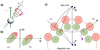Fig. 15 Cartoon model of the drift track evolution: (a) general view on the system (inside traverse geometry, pulsar is rotating clockwise), similar to Fig. 1, but with individual sparks at two different radio frequencies, νlo (red) and νhi (green). According to the RFM, emission at νlo comes fromhigher altitudes, where the opening angle of the dipole field lines is larger. The modfolds at these two frequencies are shown in (b). The carousel configuration corresponding to the moment marked with the dotted horizontal line in (b) is shown in (c). The violet arrows in (a) and (c) mark the direction of the carousel rotation (see text for more details). The black arrows show increasing longitude, ϕ, and the magnetic azimuth, ψ, both measured from the fiducial longitude. At this moment, the LOS sweeps through the spark centres at νlo and misses the spark centres at νhi. For the leading component (LC), the rotating carousel needs more time to bring the spark centre to the LOS. The drift phase Θ is directly proportional to time (Eq. (16)), thus |ΘLC(νhi)| > |ΘLC(νlo)|. The spherical triangles defined by the spin axis, magnetic axis, and the point where the LOS passes through the emission cone (black lines) are identical to the triangle in the inset of Fig. 1.

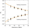Fig. 16 Black points show the drift phase ΘC vs. radio frequency for the leading and trailing drift tracks for all pulse stacks of the session L99010, where the fitted 2D Gaussians had an S∕N > 7. The orange lines mark the expected phase delay of the rotating carousel calculated according to Eq. (16).

Acknowledgements

AVB thanks the referee, Joanna Rankin (UVM), as well as Vlad Kondratiev (ASTRON), and Tim Pennucci (ELTE) for the valuable comments on the manuscript. This paper is based (in part) on data obtained with the International LOFAR Telescope (ILT). LOFAR (van Haarlem et al. 2013) is the Low Frequency Array designed and constructed by ASTRON. It has facilities in several countries, which are owned by various parties (each with their own funding sources), and which are collectively operated by the ILT foundation under a joint scientific policy.

References

All Tables

All Figures

Fig. 1 Sketch of basic magnetospheric geometry. The angular momentum $\overline{\text{Ω}}$ of the pulsar is directed vertically and the magnetic dipole vector $\overline{\mu }$ is inclined by the angle α. The angle between the spin axis and the LOS is the viewing angle ζ. The LOS vector stays fixed in space while the pulsar rotates around the spin axis in counter-clockwise direction. The sketch shows the moment in time when the magnetic dipole and LOS vectors lie on the same plane, corresponding to the fiducial rotational longitude, ϕ0. In this plane, the angle between an observer and the magnetic axis is β. Following EW01, α, and ζ are measured clockwise from the direction of $\overline{\text{Ω}}$, and β is measured clockwise from the direction of $\overline{\mu }$ (see text for more details). The thick black line shows an example of a dipolar field line, and the thick grey line marks the emission cone with an opening angle, ρ. Two components of the observed average profile are separated by ϕsep in rotational longitude. The dashed-line spherical triangle is shown in the inset, with PA being the measured position angle of the linearly polarised radiation, and ψ being the magnetic azimuth. We note that β, ζ, and ρ are usually plotted shifted to the common origin in the centre of the star (e.g. Lorimer & Kramer 2004; Fig. 3.4a). This transformation does not change the subsequent derivations in the text.

In the text

Fig. 2 Pulsar orientation angles for the two branches of our geometry fit. The pulsar rotates counter-clockwise, and the spin axis is shown by the vertical arrow. The shorter green arrows show the magnetic axis, and the brown arrows show the LOS. The branches are labelled outside traverse and inside traverse to match the notation of DR01; inside/outside refers to the relative position of the LOS direction with respect to the smaller angle between the spin and magnetic axes. We follow the definition of (α, β) in EW01, which is different from the one used by DR01. The conversion between the two notations is given in Table 2.

In the text

Fig. 3 Pulsar orientation angles based on the analysis of frequency-dependent component separation and the PA sweep rate versus the assumed value of the emission cone opening angle at 1 GHz, ρ1 GHz. The black lines show α(ρ1 GHz) and β(ρ1 GHz) for RPA = −2.9°/°. Shaded regions mark a ± 0.5°/° uncertainty in RPA, where the lower edge corresponds to a lower absolute value of RPA. The stars mark the DR01 geometry solutions corresponding to the inner and outer cone ρ1 GHz (white and black, respectively). The angles were converted into the EW01 notation according to Table 2.

In the text

	Fig. 4 Example of a drifting subpulse sequence. ${\widehat{P}}_2$ corresponds to the observed longitudinal spacing between subpulses, and ${\widehat{P}}_3$ is the amount of time between subpulses that appear at the same longitude. Here, ${\widehat{P}}_3$ is equal to the integer number of the rotation periods, but this is not necessarily true in general.
In the text

Fig. 5 Example of pulse sequences in the Q and B modes from the observing session L102418. Only the on-pulse longitude region is shown. In the B mode the apparent drift period $\left|{\widehat{P}}_3\right|$ is similar to two rotation periods, which results in the distinct even-odd modulation of the subpulses (see Sect. 6 for the discussion of the ${\widehat{P}}_3$ sign). If $\left|{\widehat{P}}_3\right|$ were exactly 2P1, drifting subpulses would appear at the same longitudes during every other rotation period. Because $\left|{\widehat{P}}_3\right|$ is slightly larger than 2P1, however, thesubpulses appear to be slowly shifting towards the leading edge of the average profile, with an apparent cycle of about 10P1.

In the text

Fig. 6 Topplot: stack of LRF power spectra, integrated within the on-pulse window. On the X-axis, each column corresponds to the LRF spectrum computed from 512-pulse (≈9 min) pulse stacks. Only the Fourier frequencies around the B-mode feature are shown. The S/N ratio is shown with colour. Similarly to B14, observations are aligned by the Q-to-B transition. Vertical solid lines mark B-to-Q transitions, and dashed lines show the Q-to-B transitions. The observed ${\widehat{P}}_3$ slowly evolves with time since the B-mode onset and also exhibits strong random fluctuation around the general trend. Bottom row: two examples of individual LRF spectra showing different types of P3 behaviour: multiple peaks (A) and a single peak (B). The average profiles for the corresponding pulse sequences are plotted in the side panel. Two solid vertical lines mark the supposed position of the sidelobes (for the highest S/N peak in A), calculated for the 20-spark carousel from DR01. The dotted line shows the first-degree alias of the second harmonic frequency of the highest S/N peak, and the dashed line marks the frequency of the supposed 37P1 modulation from Asgekar & Deshpande (2001).

In the text

Fig. 7 On-pulse averaged LRF spectra for two 512-pulse sequences (light colour, filled) together with the LRF spectra computed for the first and last 256 pulses of each pulse sequence (black, empty). Only the Fourier frequencies around the B-modefeature are shown. The pulse numbers in the legend are counted from the closest Q-to-B transition. Left: example of an LRF spectrum with two peaks that are resolved into a single peak that changes its position with time. All double features with clearly separated peaks were resolved in this way. Right: example of an LRF spectrum for a 512-pulse sequence that shows the peak offset from the peaks in the LRF spectra of the subsequences. This behaviour might be explained by phase jumps within the pulse sequence.

In the text

	Fig. 8 Primary feature of the LRF spectra from Fig. 6 for the three B-mode intervals with observed Q-to-B transitions. If the LRF spectrum had several peaks, all of them were plotted. The size of the marker corresponds to the peak S/N. The fit of Eq. (7) from Backus et al. (2011) is overplotted, which was based on two partial B-modes observed at 325 MHz.
In the text

Fig. 9 Unwrapped phase tracks, θ(ϕ) from Eq. (6) (black dots) at the Fourier frequencies corresponding to the $P_1/{\widehat{P}}_3$ peaks intwo LRF spectra with relatively strong (left) and weak (right) drifting features. The θ(ϕ) from the longitude region around the peaks of the average profile (larger markers) were used to fit the number of sparks in the carousel according to Eq. (9). Black lines mark an example of such fit performed with the standard set of geometry/aliasing parameters (see text for details), and the bottom panels show the residuals together with the fitted θ(ϕ) uncertainty. The orange line depicts the longitudinal separation between subpulses, ${\widehat{P}}_2(\varphi )$, computedby differentiating the fit line (Eq. (5)). The orange error bar at ϕ = 0 marks the ${\widehat{P}}_2$ uncertainty derived from the uncertainty in fitted N. The average profile of the pulse sequence is shown with shades of grey. For convenience, since ${\widehat{P}}_2$ is measured in degrees, the top axis shows the spin longitude ϕ in the same units.

In the text

Fig. 10 Phase tracks for the beginning (black) and the end (red) of the same B mode (observation L99010), with an artificial vertical offset added. The average profiles of the corresponding pulse sequences are plotted in the background with matching colours. The serifs mark the midpoint between profile components (see text for details). Lines show the fit with standard geometry/aliasing parameters. Solid lines correspond to the fit with fiducial longitude ϕ0 matching the midpoint between profile components. The light blue dashed line shows the fit to the late-mode phase track with ϕ0 fixed at the position of the midpoint between components at the onset of the B mode. Both constant and moving ϕ0 yield the same quality fits and an almost identical number of sparks N, and the change in ϕ0 is absorbed by fitted θ0.

In the text

Fig. 11 Reference number of sparks, N0, under different assumptions of the geometry angles and the degree of aliasing, n. N0 was obtained by fitting Eq. (9) to a single pulse stack with high S/N in session L99010. The left and right panels show N0 for the outside and inside traverse geometry branches. For each of the three values of RPA, namely − 3.4, − 2.9, and − 2.4°/°, a set of trial ρ1 GHz between 2° and 8° was used. For clarity, the points for different ρ0 are plotted with the horizontal offset proportional to ρ0 − 4.5°. Although the carousel model prescribes the integer number of sparks, N0 was not fixed to an integer value during the fit.

In the text

Fig. 12 Left: relative change in the number of sparks for every distinct peak in each of the 512-pulse LRF spectra. The fit was performed with the standard set of aliasing/geometry parameters, for the inside (black dots) and outside (purple dots) traverse geometries. The “reference” number of sparks, N0, was taken from Fig. 11. Right: ${\widehat{P}}_2$ at the fiducial longitude, ϕ0, from Eq. (11) for inside (black dots) and outside (green dots) traverse geometries.

In the text

	Fig. 13 Relative change in the number of sparks for the three frequencies within the LBA band with respect to the reference number of sparks N0 from Fig. 11. The fit at the lowest frequency yields slightly but consistently larger N.
In the text

Fig. 14 Example of a 512-pulse stack folded modulo ${\widehat{P}}_3$ for six radio frequencies within the LBA band. The modfold is repeated twice along the Y -axis to mitigate wrapping, and the corresponding average profile is plotted on top. White circles mark the centres of driftbands obtained from fitting 2D tilted Gaussians. As the radio frequency increases, the driftbands move towards each other both in ϕ (reflecting the behaviour of the average profile components) and in Θ.

In the text

Fig. 15 Cartoon model of the drift track evolution: (a) general view on the system (inside traverse geometry, pulsar is rotating clockwise), similar to Fig. 1, but with individual sparks at two different radio frequencies, νlo (red) and νhi (green). According to the RFM, emission at νlo comes fromhigher altitudes, where the opening angle of the dipole field lines is larger. The modfolds at these two frequencies are shown in (b). The carousel configuration corresponding to the moment marked with the dotted horizontal line in (b) is shown in (c). The violet arrows in (a) and (c) mark the direction of the carousel rotation (see text for more details). The black arrows show increasing longitude, ϕ, and the magnetic azimuth, ψ, both measured from the fiducial longitude. At this moment, the LOS sweeps through the spark centres at νlo and misses the spark centres at νhi. For the leading component (LC), the rotating carousel needs more time to bring the spark centre to the LOS. The drift phase Θ is directly proportional to time (Eq. (16)), thus |ΘLC(νhi)| > |ΘLC(νlo)|. The spherical triangles defined by the spin axis, magnetic axis, and the point where the LOS passes through the emission cone (black lines) are identical to the triangle in the inset of Fig. 1.

In the text

	Fig. 16 Black points show the drift phase ΘC vs. radio frequency for the leading and trailing drift tracks for all pulse stacks of the session L99010, where the fitted 2D Gaussians had an S∕N > 7. The orange lines mark the expected phase delay of the rotating carousel calculated according to Eq. (16).
In the text

References

- Asgekar, A., & Deshpande, A. 2001, MNRAS, 326, 1249 [NASA ADS] [CrossRef] [Google Scholar]
- Backer, D. C. 1970, Nature, 227, 692 [NASA ADS] [CrossRef] [Google Scholar]
- Backus, I., Mitra, D., & Rankin, J. M. 2010, MNRAS, 41, 30 [NASA ADS] [Google Scholar]
- Backus, I., Mitra, D., & Rankin, J. M. 2011, MNRAS, 418, 1736 [NASA ADS] [CrossRef] [Google Scholar]
- Bilous, A. V., Hessels, J. W. T., Kondratiev, V. I., et al. 2014, A&A, 572, A52 (B14) [NASA ADS] [CrossRef] [EDP Sciences] [Google Scholar]
- Champion, D. J., Lorimer, D. R., McLaughlin, M. A., et al. 2005, MNRAS, 363, 929 [NASA ADS] [CrossRef] [Google Scholar]
- Cordes, J. M. 1978, ApJ, 222, 1006 [NASA ADS] [CrossRef] [PubMed] [Google Scholar]
- Deshpande, A. A., & Rankin, J. M. 2001, MNRAS, 322, 438 (DR01) [NASA ADS] [CrossRef] [Google Scholar]
- Dyks, J., & Rudak, B. 2015, MNRAS, 446, 2505 [NASA ADS] [CrossRef] [Google Scholar]
- Edwards, R. T., & Stappers, B. W. 2003, A&A, 410, 961 (ES03) [NASA ADS] [CrossRef] [EDP Sciences] [Google Scholar]
- Everett, J. E., & Weisberg, J. M. 2001, ApJ, 553, 341 (EW01) [NASA ADS] [CrossRef] [Google Scholar]
- Gil, J., Gronkowski, P., & Rudnicki, W. 1984, A&A, 132, 312 [NASA ADS] [Google Scholar]
- Halpern, J. P., Bogdanov, S., & Thorstensen, J. R. 2017, ApJ, 838, 124 [NASA ADS] [CrossRef] [Google Scholar]
- Hassall, T. E., Stappers, B. W., Weltevrede, P., et al. 2013, A&A, 552, A61 [NASA ADS] [CrossRef] [EDP Sciences] [Google Scholar]
- Hermsen, W., Hessels, J. W. T., Kuiper, L., et al. 2013, Science, 339, 436 [NASA ADS] [CrossRef] [Google Scholar]
- Kondratiev, V. I., Verbiest, J. P. W., Hessels, J. W. T., et al. 2016, A&A, 585, A128 [NASA ADS] [CrossRef] [EDP Sciences] [Google Scholar]
- Lorimer, D. R., & Kramer, M. 2004, Handbook of Pulsar Astronomy, (Cambridge, UK: Cambridge University Press) [Google Scholar]
- Lyne, A. G., & Manchester, R. N. 1988, MNRAS, 234, 477 [NASA ADS] [CrossRef] [Google Scholar]
- Mereghetti, S., Kuiper, L., Tiengo, A., et al. 2016, ApJ, 831, 21 [CrossRef] [Google Scholar]
- Mereghetti, S., & Rigoselli, M. 2017, J. Astrophys. Astron., 38, 54 [NASA ADS] [CrossRef] [Google Scholar]
- Mitra, D., & Deshpande, A. A. 1999, A&A, 346, 906 (MD99) [NASA ADS] [Google Scholar]
- Noutsos, A., Sobey, C., Kondratiev, V. I., et al. 2015, A&A, 576, A62 [NASA ADS] [CrossRef] [EDP Sciences] [Google Scholar]
- Radhakrishnan, V., & Cooke, D. J. 1969, Astrophys. Lett., 3, 225 [NASA ADS] [Google Scholar]
- Rankin, J. M. 1990, ApJ, 352, 247 [NASA ADS] [CrossRef] [Google Scholar]
- Rankin, J. M. 1993a, ApJ, 405, 285 [NASA ADS] [CrossRef] [Google Scholar]
- Rankin, J. M. 1993b, ApJS, 85, 145 [NASA ADS] [CrossRef] [Google Scholar]
- Rankin, J., & Rosen, R. 2014, MNRAS, 439, 3860 [NASA ADS] [CrossRef] [Google Scholar]
- Rankin, J. M., & Suleymanova, S. A. 2006, A&A, 453, 679 [NASA ADS] [CrossRef] [EDP Sciences] [Google Scholar]
- Rankin, J. M., Suleymanova, S. A., & Deshpande, A. A. 2003, MNRAS, 340, 1076 [NASA ADS] [CrossRef] [Google Scholar]
- Rankin, J. M., Ramachandran, R., & Suleymanova, S. A. 2005, A&A, 429, 999 [NASA ADS] [CrossRef] [EDP Sciences] [Google Scholar]
- Rosen, R., & Clemens, J. C. 2008, ApJ, 680, 671 [NASA ADS] [CrossRef] [Google Scholar]
- Ruderman, M. A., & Sutherland, P. G. 1975, ApJ, 196, 51 [NASA ADS] [CrossRef] [EDP Sciences] [Google Scholar]
- Suleymanova, S. A., & Izvekova, V. A. 1984, Soviet Ast., 28, 32 [NASA ADS] [Google Scholar]
- Suleymanova, S. A., & Rankin, J. M. 2009, MNRAS, 396, 870 [NASA ADS] [CrossRef] [Google Scholar]
- Suleymanova, S. A., & Rodin, A. E. 2014, Astron. Rep., 58, 796 [NASA ADS] [CrossRef] [Google Scholar]
- Suleymanova, S. A., Izvekova, V. A., Rankin, J. M., & Rathnasree, N. 1998, J. Astrophys. Astron., 19, 1 [NASA ADS] [CrossRef] [Google Scholar]
- Szary, A., & van Leeuwen J. 2017, ApJ, 845, 95 [NASA ADS] [CrossRef] [Google Scholar]
- Szary, A., Melikidze, G. I., & Gil, J. 2015, MNRAS, 447, 2295 [NASA ADS] [CrossRef] [Google Scholar]
- Taylor, J. H., & Huguenin, G. R. 1971, ApJ, 167, 273 [NASA ADS] [CrossRef] [Google Scholar]
- Timokhin, A. N. 2010, MNRAS, 408, L41 [NASA ADS] [CrossRef] [Google Scholar]
- van Haarlem, M. P., Wise, M. W., Gunst, A. W., et al. 2013, A&A, 556, A2 [NASA ADS] [CrossRef] [EDP Sciences] [Google Scholar]
- van Leeuwen, J., & Timokhin, A. N. 2012, ApJ, 752, 155 [NASA ADS] [CrossRef] [Google Scholar]
- van Straten, W., Manchester, R. N., Johnston, S., & Reynolds, J. E. 2010, PASA, 27, 104 [NASA ADS] [Google Scholar]
- Vitkevich, V. V., Alekseev, Y. I., Zhuravlev, V. F., & Shitov, Y. P. 1969, Nature, 224, 49 [NASA ADS] [CrossRef] [Google Scholar]
- Weltevrede, P., Edwards, R. T., & Stappers, B. W. 2006, A&A, 445, 243 [NASA ADS] [CrossRef] [EDP Sciences] [Google Scholar]
- Yuen, R., Melrose, D. B., Samsuddin, M. A., Tu, Z. Y., & Han, X. H. 2016, MNRAS, 459, 603 [NASA ADS] [CrossRef] [Google Scholar]
All Tables
Relationship between the conventions for inclination angle α and impact angle β in DR01 and EW01 for the outside traverse and inside traverse branches of the geometry fit in DR01.