| Issue |
A&A
Volume 615, July 2018
|
|
|---|---|---|
| Article Number | A178 | |
| Number of page(s) | 15 | |
| Section | Interstellar and circumstellar matter | |
| DOI | https://doi.org/10.1051/0004-6361/201732562 | |
| Published online | 07 August 2018 | |
Catching drifting pebbles
II. A stochastic equation of motion for pebbles
Anton Pannekoek Institute (API), University of Amsterdam,
Science Park 904,
1090 GE
Amsterdam,
The Netherlands
e-mail: This email address is being protected from spambots. You need JavaScript enabled to view it.
; This email address is being protected from spambots. You need JavaScript enabled to view it.
Received:
29
December
2017
Accepted:
27
March
2018
Abstract
Turbulence plays a key role in the transport of pebble-sized particles. It also affects the ability of pebbles to be accreted by protoplanets because it stirs pebbles out of the disk midplane. In addition, turbulence suppresses pebble accretion once the relative velocities become too high for the settling mechanism to be viable. Following Paper I, we aim to quantify these effects by calculating the pebble accretion efficiency ε using three-body simulations. To model the effect of turbulence on the pebbles, we derive a stochastic equation of motion (SEOM) applicable to stratified disk configurations. In the strong coupling limit (ignoring particle inertia) the limiting form of this equation agrees with previous works. We conduct a parameter study and calculate ε in 3D, varying pebble and gas turbulence properties and accounting for the planet inclination. We find that strong turbulence suppresses pebble accretion through turbulent diffusion, agreeing closely with previous works. Another reduction of ε occurs when the turbulent rms motions are high and the settling mechanism fails. In terms of efficiency, the outer disk regions are more affected by turbulence than the inner regions. At the location of the H2O iceline, planets around low-mass stars achieve much higher efficiencies. Including the results from Paper I, we present a framework to obtain ε under general circumstances.
Key words: planets and satellites: formation / protoplanetary disks / methods: numerical
© ESO 2018
1 Introduction
It is widely believed that turbulence plays an important role in the evolution of protoplanetary disks. For a long time, the magneto-rotational instability (MRI; Balbus & Hawley 1991) has been regarded as the leading candidate in driving the disk’s angular momentum transport. More recently, disk wind models have regained traction (Bai et al. 2016; Suzuki et al. 2016; Gressel 2017), where the turbulence in the midplane regions is limited to hydrodynamic instabilities such as the vertical shear instability (Nelson et al. 2013; Stoll & Kley 2014). Turbulence, in addition, is important in shaping the outcome of the early coagulation process. Already at low Mach numbers, turbulence dominates the relative velocity between particles (Völk et al. 1980; Ormel & Cuzzi 2007; Pan & Padoan 2010). It is also the only explanation for why we infer vertical structure (e.g., flared versus settled geometry), since turbulence allows small particles to be lifted from the disk midplane regions. Indeed, with the current state-of-the-art models small (micron-size) particles are produced in the midplane through collisions between pebbles and boulder sized particles before they diffuse upwards (Birnstiel et al. 2010, 2011; Krijt & Ciesla 2016).
Because of its subsonic nature, obtaining observational evidence of turbulence is hard. Disks like TW Hya, HD 163296, and DM Tau have been modeled by several groups (Hughes et al. 2011; Guilloteau et al. 2012; Flaherty et al. 2015, 2017) with turbulent Mach numbers inferred from the rather quiescent ~0.01 to the more vigorous ~0.1. However, it should be emphasized that constraining the turbulent rms velocity (σ) by these single-line profiles requires that the temperature profile be known to great precision. Generally, uncertainties affecting σ are limited by the absolute flux calibration and spectral resolving power (Teague et al. 2016). More indirect methods of obtaining σ employ the appearance of the dust disk in ALMA imagery. Applied to HL tau this indicates that the pebbles are settled into the midplane, resulting in a vertical turbulent diffusivity parameter αz~10−4 (Pinte et al. 2016)1. Flock et al. (2017) conclude this is consistent with a magnetized disk models that feature a “dead” midplane.
Both classical planetesimal-driven models for planet formation (Safronov 1969; Pollack et al. 1996) as well as the more recent pebble accretion model (Ormel & Klahr 2010; Lambrechts & Johansen 2012) are greatly affected by turbulence. Both models operate best under low-turbulence conditions. The runaway growth phase for the classical, planetesimal-driven accretion paradigm can only operate once the planetesimals start out with close to zerovelocity dispersions, but stochastic forcing by turbulence-triggered density fluctuations (Ida et al. 2008; Nelson & Gressel 2010; Gressel et al. 2011, 2012; Okuzumi & Ormel 2013) excites planetesimals to random velocities higher than their escape velocity. This implies that planetesimals have to be born large or that turbulence has to be weak (Ormel & Okuzumi 2013; Kobayashi et al. 2016). Similarly, the efficacy of pebble accretion to grow planets also depends on the turbulence. As pebbles will be stirred away from the midplane, it reduces the number of pebbles left to be accreted (Ormel & Klahr 2010; Guillot et al. 2014; Morbidelli et al. 2015). A second, less known, effect is that turbulent forcing may provide particles with an additional relative motion, which could also suppress accretion.
In this work, we consider simultaneously the effects of turbulent diffusivity and turbulent velocity. We do this by deriving a stochastic equation of motion (SEOM) for pebble-sized particles. Simply put, the SEOM is an extension of the Newtonian equation of motion, but with an additional stochastic component. For planets, stochastic forces have been invoked as a means to cross mean motion resonances (Rein & Papaloizou 2009; Paardekooper et al. 2013). As detailed by Rein & Papaloizou (2009), the stochastic motion is characterized by two parameters: the diffusivity DP and the correlation time tcorr. The latter iscrudely the time over which the stochastic force changes its direction. For pebbles, we adopt a similar model, where now the stochastic motions are driven by aerodynamical coupling to the turbulent gas. However, in the few studies that have considered stochastic effects for pebble-sized particles, it is often assumed that turbulence does not feature a correlation time, i.e., tcorr is assumed less than any other timescale in the problem (Ciesla 2010; Zsom et al. 2011; Krijt & Ciesla 2016). This implies “white noise” behavior, i.e., that the particle is displaced in a random direction at every time. This approximation is known as the strong coupling limit (SCA).
A key goal of this paper is to test how the SCA fares in the light of the more accurate SEOM. We find that the SCA is generally applicable, as long as both the particle stopping time tstop and the turbulent correlation time are sufficiently small. In addition, we will study the effect of a vertically varying turbulent gas diffusivity, Dzz(z), to investigate when it is viable to stir a fraction of pebble size particles to the disk surface.
Our main thrust will be to apply the SEOM and the SCA methods to calculate pebble accretion efficiencies in three-dimensional (3D) settings. In Liu & Ormel (2018, henceforth Paper I) we have defined ε as the probability that a pebble, drifting towards the star, will be accreted by a single planet(esimal)2. A very small value of ε implies that a large number of pebbles are needed to grow the planet, while ε close to unity implies that pebble accretion is a very efficient accretion process. In Paper I we used planar 3-body calculation (star, planet, pebble) to calculate ε in two dimensions. We then investigated how this ε2D changed as function of planet properties (mass and eccentricity), disk properties (position, radial drift velocity), and pebble properties (stopping time). In this work, we extend these calculation to the vertical dimension by including the planet’s inclination and disk turbulence. With the ε3 D of this paper and the ε2D of Paper I, we then obtain a general recipe for the pebble accretion efficiency (ε) of a single planet.
The plan of the paper is the following. In Sect. 2 we derive the SEOM. This section, as well as Appendix A, are rather technical and may be skipped by readers more interesting in the physical applications. In Sect. 3 we apply our newly developed SEOM to find vertical density distributions and show that our results are consistent with previous numerical and analytical studies. We apply the SEOM and SCA to pebble accretion in Sect. 4. We find ε for a variety of settings (planet mass and inclination, particle and disk properties) and present a framework to obtain ε under general circumstances (including the results found in Paper I). A comparison with previous studies is presented in Sect. 5. We summarize our findings in Sect. 6.
2 Model
2.1 Advection-diffusion equation
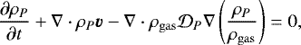
In this workwe model turbulence motion of particles and gas by an advection-diffusion equation:
 (1)
(1)
where ρP is the density of particles or gas species, v the systematic (drift) velocity, ρgas the gas density, and  the particle diffusivity tensor whose elements are denoted Dij. Importantly, the diffusion term acts on the gradient of the concentration (ρP ∕ρgas): it tends to erase concentration gradients and vanishes when the concentration is uniform.
In this work, we will restrict diffusion to operate only in the vertical (z) direction, considering only DP,zz. Furthermore, we adopt the vertically isothermal solution for the gas density
![Mathematical equation: \begin{equation*} \rho_{\mathrm{gas}} = \frac{\mathrm{\Sigma}_{\mathrm{gas}}}{H_{\mathrm{gas}}\sqrt{2\pi}} \exp \left[ -\frac{1}{2} \left( \frac{z}{H_{\mathrm{gas}}} \right)^2 \right],\end{equation*}](/articles/aa/full_html/2018/07/aa32562-17/aa32562-17-eq3.png) (2)
(2)
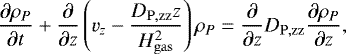
where Σgas is the gas surface density and Hgas the pressure scaleheight. Under these conditions, Eq. (1) can be manipulated:
 (3)
(3)
(Ciesla 2010)3. For small particles (including pebbles), the vertical velocity vz equals the settling velocity, vz = −zΩ2tstop with tstop the stopping time and Ω the Keplerian orbital frequency. The gas density no longer appears in Eq. (3), but the diffusivity appears at two places. On the RHS the diffusive term is responsible for spreading the particle concentration, resulting in a broader distribution of ρP (z). However, the additional advection term  – a consequence of imposing Eq. (2) – counteracts this, enforcing the particle layer to remain stratified with a finite dispersion at all times (Ciesla 2010).
For a distribution of particles ρP(z)dz∕Σ gives the fraction of the particles within the interval [z, z + dz]. For a single particle, P(z) = ρ(z)∕Σ similarly denotes the probability of finding the particle within [z, z + dz] where P(z) is the probability density. We will use this identification below to obtain the correct, statistical properties of our single-particle (Lagrangian) stochastic model.
2.2 Stochastic equation of motion (SEOM)
The stochastic equation of motion is given by the following set of stochastic differential equations (SDEs):
 (4a)
(4a)
 (4b)
(4b)
 (4c)
(4c)
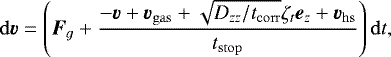
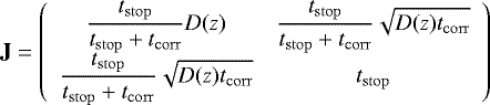
where x is the position andv is the velocity of a particle. The particle is subject to gravitational forces Fg and gas drag forces. The latter have been expressed in terms of the stopping time, Δv∕tstop, where Δ v is the relative gas-particle velocity. In Eq. (4c), Wt denotes a Wiener process (Brownian motion) and the corresponding differential is 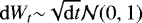 where
where  is the normal distribution with zero mean and unity variance.
Apart from v, three velocity terms appear in Eq. (4b):
- 1.
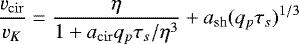
A laminar gas velocity vgas. In our case, the gas velocity operates in the azimuthal direction
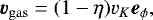 (5)
(5)where
 and η represents the disk radial pressure gradient:
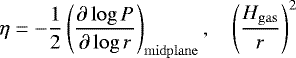 (6)
(6)is assumed constant (Nakagawa et al. 1986).
- 2.
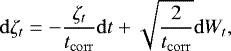
A turbulent velocity vturb. In Eq. (4b) this has been written in terms of an rms value (
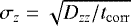 ) and a non-dimensional stochastic variable ζt. Here tcorr and Dzz are, respectively, the correlation time and diffusivity of the turbulent gas. In Eq. (4b) the turbulent forcing acts only in the vertical dimension.
 - 3.
A correction term vhs
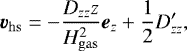 (7)
(7)where
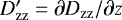 . This is needed to enforce that Eq. (4) satisfies the hydrostatic balance condition, which assumption has entered the advection-diffusion equation (Eq. (3)). It also accounts for spatial gradients in Dzz. We derive it below.
Finally, Eq. (4c) is a stochastic differential equation (SDE) about a quantity ζt. This can be thought of as the normalized strength of the turbulent velocity. Specifically, Eq. (4c) describes an Ornstein–Uhlenbeck process (Uhlenbeck & Ornstein 1930) with zero mean (⟨ζt ⟩ = 0), unity variance ( ) and correlation time tcorr. On long timescales ζt will be normally distributed; events separated by Δt ≫ tcorr are uncorrelated. However, times separated by Δt ≪ tcorr will feature a similar value of ζt and hence a similar turbulent gas velocity.
2.3 Turbulent correlation time
In Eq. (4) we are at liberty to choose tcorr, which can be identified with the correlation time (or lifetime) of the turbulent eddies. A smaller tcorr (while keeping Dzz fixed) implies a more vigorous turbulent forcing (larger σz), while a long tcorr implies that the turbulence is characterized by weaker but larger and longer-lived eddies. It is customary to adopt the Shakura & Sunyaev (1973) α-parameterization for the turbulent viscosity:
 (8)
(8)
We will adopt a similar parameterization for the gas diffusivity, i.e.,  where αz reflects the diffusivity of the gas, not angular momentum transport. Using
  , the turbulent rms velocity becomes
 (9)
(9)
Following Dubrulle et al. (1995), Cuzzi et al. (2001) and Johansen et al. (2006), we usually adopt tcorr = Ω−1 and hence  . In Sect. 3.2 we also consider models where tcorr is longer.
The following qualifications will be adopted towards the turbulence strength:
laminar for αz = 0;
-
weakly turbulent for αz < 10−4;
moderately turbulent for 10−4 < αz < 10−2;
-
strongly turbulent for αz > 10−2.
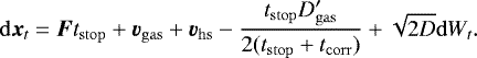
2.4 Strong coupling approximation (SCA)
The strong coupling applies when tstop is small. In that limit, it can be shown that Eq. (4) simplifies into a single SDE for the position:
![Mathematical equation: \begin{equation*}\mathrm{d}\bm{x} = \left[ \bm{F}t_{\mathrm{stop}} +\bm{v}_{\mathrm{gas}} +\bm{v}_{\mathrm{hs}} +\frac{D'_{\mathrm{zz}}\bm{e}_z}{2(1+t_{\mathrm{stop}}/t_{\mathrm{corr}})} \right] \mathrm{d} t +\sqrt{2D_{\mathrm{zz}}} \bm{e}_z \mathrm{d} W_t, \end{equation*}](/articles/aa/full_html/2018/07/aa32562-17/aa32562-17-eq23.png) (10)
(10)
(see Appendix A for the derivation). In Eq. (10), we have allowed Dzz to depend on position, which would give rise to an additional advective term (the fourth term in the square brackets). Equation (10) is analogous to Smoluchowski (1916) equation for the stochastic motion of a massless particle subject to a fluctuating force.
We arenow in a position to obtain the hydrostatic correction term vhs. SDEs of the form
 (11)
(11)
can equivalently be cast in terms of an equation for the evolution of the probability density P(x, t) – i.e., a Fokker–Planck equation
 (12)
(12)
(van Kampen 1992)4. Applied to Eq. (10), the Fokker–Planck equation for the probability density P(z, t) reads
 (13)
(13)
where we consider the limit tstop ≪ tcorr. The RHS of Eq. (13) can be expanded as  . Identifying the probability density P(z) with the density ρP of Eq. (3), Fztstop with vz, and using that DP,zz = Dzz for strongly coupled particles (Völk et al. 1980), we obtain the hydrostatic correction term, Eq. (7). With this correction term, the SCA for the particle position in 1D reads
![Mathematical equation: \begin{equation*} \mathrm{d} z = \left[-z \mathrm{\Omega}^2 t_{\mathrm{stop}} -\frac{D_{\mathrm{zz}} z}{H_{\mathrm{gas}}^2} +D_{\mathrm{zz}}'\right]\mathrm{d} t +\sqrt{2D_{\mathrm{zz}}}\, \mathrm{d} W_t\end{equation*}](/articles/aa/full_html/2018/07/aa32562-17/aa32562-17-eq28.png) (14)
(14)
as was already derived by Ciesla (2010) and also used in Zsom et al. (2011) and Charnoz et al. (2011). Comparing the second and third terms on the RHS, we obtain that the turbulent gradient effect becomes important when Dzz changes on scales less than  .
.
We reflect on our findings. Equation (10) with vhs equal to Eq. (7) describesthe stochastic motion of a particle experiencing drag and turbulent forces, with the turbulence characterized by a correlation time tcorr and a (possibly spatially dependent) gas diffusivity Dzz. Under the assumption of small tstop and small tcorr, we obtain Eq. (14), consistent with Ciesla (2010). However, these equations provide no model for the particle velocity; and they will fail when the SCA conditions no longer materialize (long tstop or long tcorr) – i.e., when the particle’s inertia matters. In these cases, Eq. (4) provides a more general description of stochastic motion of pebble-sized particles.
3 Vertical diffusion
We test our algorithms – the stochastic equation of motion (SEOM; Eq. (4)) and the strong coupling approximation (SCA; Eq. (14)) – for tracer particles (tstop = 0) in Sect. 3.1 and massive particles (Sect. 3.2) for a variety of stopping times and αz.
3.1 Tracer particle
Tracer particles should have a vertical distribution identical to the gas, Eq. (2). Because tstop = 0 for tracer particles, the SEOM, as described in Eq. (4), contains a singularity and is not applicable. Therefore, we adopt the SCA method. In Eq. (10) we take tstop = 0, η = 0,  . The choices for Hgas and Ω are arbitrary.
In Fig. 1a we show the distribution of the vertical position of a single particle for αz = 10−4, 10−3 and 10−2. These have been obtained by storing the vertical positions after every 1 Ω−1 for a total time of tmax = 105 Ω−1. In addition, we plot the expected distribution according to Eq. (2). The distributions are normalized such that they integrate to unity. Clearly, the distributions among the αz differ, with αz = 10−2 best matching the expected normal distribution αz = 10−4 the worst. The origin of these differences is the different number of independent samples that are obtained among the αz. Since our sampling time is only Δ t = 1 Ω−1, much smaller than the diffusion time tdiff = 1∕αzΩ, sequential samples (in time) will be strongly correlated; only tmax∕tdiff = 105αz samples will be independent. Hence, the higher α, the better the correspondence to a Gaussian distribution.
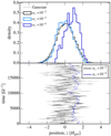 |
Fig. 1 Top panel: normalized distributions of the vertical position z for the integration of the tracer case, using the strong coupling approximation (SCA) with tstop = 0. The vertical height z is recorded after every 1 Ω−1 for t = 105 Ω−1. Bars give the simulated distribution while the analytic – normal – distribution is shown by the black dashed line. Bottom panel: temporal evolution of the vertical position for αz = 10−2 (black) and αz = 10−2 (blue). |
3.2 Massive particle
Next we consider the vertical distribution of massive particles (tstop > 0), obtained bythe SEOM and the SCA methods. This means that in Eq. (4) we put Fg = −Ω2zez. We further take tcorr = 1 Ω−1 unless mentioned otherwise. Integrations ran for 106 Ω−1 and the sampling period was Δt = 10 Ω−1. The results are shown in Fig. 2. We fix αz = 10−2 but vary τs = tstopΩ = 10−2 (left panel), 10−1 (center panel), and 100 (right panel).
In all panels we compare the results for the SEOM (gray curves) with the SCA of Eq. (10) (blue). The thin black curve corresponds to a normal distribution with pebble aspect ratio:
 (15)
(15)
(Youdin & Lithwick 2007)5, where hgas = Hgas∕r and
 (16)
(16)
In the limit of Ωtcorr ≪ 1 or  , ξ ≈ 1 and the pebble aspect ratio reduces to
  (Dubrulle et al. 1995).
For small stopping times (τs = 10−2; left panel) the SCA and the SEOM overlap. From a numerical perspective the SCA is preferable as it is computationally much less intensive than the SEOM-method. For τs = 10−1, the distributions slightly differ, as can best be seen from the lower panels. For τs = 1 particles the differences between the two methods amount to several tens of percents at z = 0, while towards the tails of the distribution the relative difference is larger even. The SEOM, however, is in perfect agreement with the Youdin & Lithwick (2007) theory on diffusive transport. The reason is that, like Youdin & Lithwick (2007), the SEOM accounts for the vertical oscillation (epicyclic motion) of particles, whereas the SCA does not. The SCA does not account for the pebble’s inertia and also does not involve a correlation time. From Eq. (15), we deduce that the SCA becomes invalid for  .
.
In the above, we assumed that tcorr ≈Ω−1, which is applicable in the ideal limit of MRI-turbulence (Sano et al. 2004; Johansen et al. 2006; Carballido et al. 2011). However, for non-ideal effects as ambipolar diffusion, the correlation time is expected to be longer (Bai & Stone 2011; Zhu et al. 2015). From Eq. (15), it is clear that pebbles will be more strongly stratified for large values of the turbulent correlation time tcorr. In Fig. 2b, a case with a 10 times longer correlation times (but still the same αz = 10−2 vertical diffusivity, implying larger, longer-lived but less vigorous eddies) is presented. Its vertical distribution is much narrower than the canonical tcorr = 1 Ω−1 turbulence. A case with tcorr = 102 Ω−1 is also shown in Fig. 2c. Clearly, a degeneracy between turbulent correlation time tcorr, diffusivity (αz), and stopping time (tstop) is present.
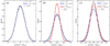 |
Fig. 2 Vertical distribution for particles of different stopping times: τs = tstopΩ = 10−2 (panel a), 10−1 (panel b), and 1 (panel c). Histograms plot the numerically obtained distributions with the stochastic equation of motion (SEOM; gray and red) and strong coupling approximation (SCA; blue) methods. Long tcorr runs are shown with red histograms (the tcorr = 102 Ω−1, τs = 0.1 run is displayed in panel c). Thin curves gives the normal distribution with the scaleheight of Eq. (15) (Youdin & Lithwick 2007). Note the different scaling among the panels. |
3.3 Vertical gradient in the diffusivity
As an application of a more convoluted model, we consider a vertically dependent diffusion. In terms of αz we adopt
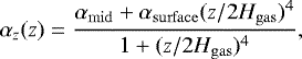 (17)
(17)
where αmid is the diffusivity in the midplane and αsurface is the diffusivity in the upper regions. Such layered accretion (Gammie 1996) when the turbulence is confined to the upper regions, although our parameterization in Eq. (17) is completely arbitrary. We choose αsurface = 0.1 and αmid = 10−3. This profile is plotted in Fig. 3 by the red curve. We further choose τs = 10−2, such that τs ∕αz > 1 in the midplane (indicating settling) and τs ∕αz < 1 in the upper regions (indicating coupling to the gas).
In Fig. 3 the gray and black histograms show the normalized distribution of z obtained with the SCA and SEOM methods, respectively. The methods give consistent result. Clearly, the high |z| regions are sparsely sampled as the probability to find a particle at these heights is low. However, the fact that pebbles can be stirred to these heights at all may be surprising given the low αmid. This is illustrated with the dark blue curve in Fig. 3, which plots P(z, hmid) where  . In fact, pebbles at |z| ≳ 2Hgas follow the gas distribution (light blue curve). Altogether P(z) can be approximated as the sum of two distributions. The majority of the pebbles (≈90%) follow the midplane distributions (given by hmid), but about 10% of the pebbles follow the distribution given by the gas scaleheight.
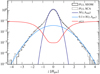 |
Fig. 3 Density distribution P(z) obtainedfrom a vertically varying diffusivity. The diffusivity profile in terms of αz is given by the red curve. The particle stopping time is τs = 10−2 and is taken independent of z. The distributions obtained from integrating the stochastic equation of motions (Eq. (4); black histogram) and the strong coupling approximation (Eq. (10); gray histograms) are consistent. The dark blue curve gives the normal distribution, for the particle scaleheight evaluated in the midplane (i.e., Eq. (15) with α = 10−3). The light blue curves gives the gas distribution, scaled by a factor 0.1. |
3.4 Local replenishment of small grains?
The ability of turbulence to stir ~mm-sized pebbles from the midplane to many gas scaleheights may offer an explanation for the persistent presence of small, (sub)micron size particles in the disk surface, as deduced from near-IR observations (e.g., Juhász et al. 2010). From a theoretical perspective, the presence of small particles is problematic as they should quickly coagulate among themselves and then settle to the disk midplane (Nakagawa et al. 1986; Tanaka et al. 2005; Dullemond & Dominik 2005). This implies that the grains are replenished. The most common theory postulates that the replenishment occurs in the disk midplane regions. Here grains are produced by high-velocity collisions among pebble-sized particles, which are subsequently transported (by diffusion) to the disk surface (Birnstiel et al. 2010). However, this is a rather indirect route to replenish small grains. First, it is doubtful if pebbles in the midplane will fragment; the gas may not be sufficiently turbulent. Second, it takes grains a time ~ 1∕αzΩ to diffuse, which is rather long, again when αz is small; these small grains may simply collide before reaching the surface (Krijt & Ciesla 2016).
Alternatively, in a disk with a suitable diffusivity profile (αz (z)), it is possible to diffuse a small number of pebbles to the disk surface. There, due to the much stronger turbulent velocity field as compared to the midplane, collisions will undoubtedly be catastrophic. To cement these ideas, a coupled transport-collision/fragmentation model need to be considered.
4 3D pebble accretion
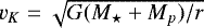
Following Paper I we calculate the accretion efficiency (ϵ) by conducting a series of N-body integrations to follow the trajectory of pebbles as they drift from orbits exterior to the planet to orbits interior to it. The pebble accretion efficiency ϵ is then found simply by counting the fraction of particles that settle to the planet. While Paper I investigated the role of the planet’s eccentricity, we fix ep = 0 here and instead investigate the role of turbulence and the planet inclination (Sect. 4.5). To this effect, we let the pebble experience a stochastic motion in the vertical direction, as outlined in Eq. (4). The initial vertical position zini is given by the steady-state distribution characterized by the pebble scaleheight hP. The initial radial position is set by
 (18)
(18)
where  is the impact parameter for pebble accretion in the Hill regime and Δrsyn(τs, η, N) the distance a pebble drifts after N synodical orbits6. We choose N = 3. When the pebble radius has drifted to a distance rp − rHill, we stop the calculation. It is then counted as a miss.
The fact that particles are only kicked in the z-direction, allows us to restrict the computations to a narrow ring. In contrast, when we would have considered the general case (turbulence operating inall dimensions), a much larger computational domain would be required because of the possibility of multiple encounters (similar to the eccentric case in Paper I). This complication is the key reason why we consider only turbulence in the vertical dimension.
Similar to Paper I, we express lengths in terms of the disk radius rp and times in units of Ω−1.
The keyparameters are as follows:
qp = Mp∕M⋆ the planet-to-stellar mass ratio;
hgas = Hgas∕r the disk aspect ratio at the location of the planet;
η, a measure of the radial drift velocity of the pebbles (Eq. (6));
τs = tstopΩ, the dimensionless stopping time;
αz, a proxy for the gas vertical diffusivity Dzz;
tcorr, the turbulent correlation time, which together with αz determines the magnitude of the turbulent rms velocities, Eq. (9).
Analogous to Paper I, we consider two integration methods:
-
The SEOM, which integrates the particle velocity (Eq. (4)).
-
The hybrid method, which uses the SCA, but switches to the SEOM when the particle is in the vicinity of the planet. Here we take the criterion to switch to the SEOM to be
 , where Δx
and Δy
are the distances between the planet and pebble in the x
and y
Cartesian coordinates. Note the absence of the vertical position in this criterion. The reason is that for some parameter combinations (small planet mass and high αz) the vertical step size can easily become larger than the Hill radius in the SCA method.
, where Δx
and Δy
are the distances between the planet and pebble in the x
and y
Cartesian coordinates. Note the absence of the vertical position in this criterion. The reason is that for some parameter combinations (small planet mass and high αz) the vertical step size can easily become larger than the Hill radius in the SCA method.
As explained in Paper I, the SCA assumes that gas and particles are well coupled. It does not capture effects that take place on timescales Δ t less than tstop + tcorr. On small Δt the particle moves ballistically, while the SCA model keep exhibiting random walk behavior at all (time)scales. Within the Hill sphere, where the numerical timestep will become small, the particle trajectories are therefore incorrect. The strong fluctuations in velocity space also complicates the numerical integration.
Different from Paper I, we do not account for the ballistic regime. Ballistic encounters are encounters in which the pebble is not captured by the settling mechanism, but where accretion occurs by virtue of the pebble hitting the surface of the target. Computationally, we can easily distinguish between ballistic and settling encounters by assigning an arbitrary small physical size to the planet (while keeping its mass). All accretion then occurs through the settling mechanism.
4.1 Standard model and analytical fits
For the standard model we take qp = 3 × 10⁻⁷ (a 0.1 M⊕ mass planet for a solar-mass star), η = 10−3, hgas = 0.03, tcorr = Ω−1 and vary αz and τs. The choices for η and hgas approximately correspond to a disk location of 1 au; both values will generally be higher in the outer disk. In Fig. 4 symbols give the mean value of ε obtained from our numerical integrations, ε = Nset∕Ntot, where out ofNtot integrations Nset pebbles settled to the planet. Error bars correspond to the Poisson error,  . The pebble accretion efficiency can be converted into the pebble growth mass, MP,grw, defined as
 (21)
(21)
(values labeled on the right y-axis). This is the amount of pebbles needed to e-fold the planet’s mass. Finally, solid curves gives our fit to the data, which will be discussed in the subsequent sections and summarized in Sect. 4.7. The fitting expression is appropriate only for τs ≲ 1.
Clearly, where ε is higher, fewer integrations are needed to obtain a minimum signal-to-noise. In our integrations Ntot is not fixed, but different for each run in order to obtain a certain signal-to-noise ratio, which is determined by the number of settling encounters. Hence, most of the computational effort is spent in the runs where ε is small. Results of the SEOM method are shown by the open circles, while the crosses (slightly offset) denote the results from the hybrid method. The two methods give consistent results (see also Paper I). For small τs the SEOM method becomes computationally inefficient as it takes the pebble a long time to drift to the interior disk and the integration becomes very stiff. The hybrid method removes this latter problem and is the method of choice for small τs. Remarkably, the hybrid method gives acceptable results up to τs = 0.5.
Results for the non-turbulent (2D) limit (αz = 0; black and gray symbols) were already discussed in Paper I. The efficiency decreases towards increasing particle stopping times – τs = 1 particles are accreted at the lowest efficiency – because the faster drift by the higher τs particles outweighs the larger linear cross section. Consequently, the pebble growth mass MP,grw is large; many pebbles are needed in order to grow the planet. The steepening of the slope that can be noticed at small τs is the result of a transition from the shear regime (velocities dominated by the Keplerian shear) at high τs to the headwind regime (velocities dominated by the gas sub-Keplerian motion, ηvK) at small τs.
When αz > 0 (colored symbols) pebbles are stirred to higher regions, reducing the local density of pebbles in the midplane. This reduces ε with respect to the 2D case. As can be seen in Fig. 4 pebbles are most affected when they are small (τs ≪ 1) and when the turbulence is strong (high αz), which is of course natural. Hence, in the 3D case there is a preferred pebble aerodynamic size where ε(τs) peaks, which occurs approximately at the point when the pebble accretion impact parameter equals the pebble scaleheight, i.e., at the transition of the 2D and 3D regimes. For heavier particles ε decreases because of more rapid radial drift, whereas for small particles ε decreases because of a reduced local density. However, when αz ≳ τs the pebble scaleheight has reached that of the gas, hP ≈ hgas, and no further reduction is possible. As a result, the curves eventually converge when τs becomes very small, as is seen in Fig. 4 in the bottom-left corner.
In Ormel (2017), as well as Paper I, we derived that the pebble accretion efficiency in the 3D limit reads
 (22)
(22)
where A3 is a numerical constant, hP the pebble aspect ratio, and fset – the settling fraction – a modulation factor which becomes less than unity when the settling criteria (slow encounters) is no longer fulfilled. The characteristic velocity beyond which settling encounters disappear is
 (23)
(23)
(Ormel & Klahr 2010; Paper I). Qualitatively, when the approach velocity7 Δ v ≪ v* settling is fully operational (fset = 1), while for Δ v ≫ v* settling (and therefore pebble accretion) are no longer viable (fset = 0). Quantitatively, the settling modulation function is fitted empirically by an exponential function (Ormel & Klahr 2010; Visser & Ormel 2016). In Paper I we adopted
![Mathematical equation: \begin{equation*} f_{\mathrm{set,I}} = \exp \left[ -a_{\mathrm{set}} \left( \frac{\mathrm{\Delta} v}{v_{\ast}} \right)^2 \right].\end{equation*}](/articles/aa/full_html/2018/07/aa32562-17/aa32562-17-eq45.png) (24)
(24)
with aset = 0.5. The subscript “I” indicates that this expression is valid for a laminar disk (Paper I). We will refine it below (Sect. 4.6) accounting for a turbulence velocity field.
The reduction of ε by fset enters quadratically in 3D because the cross section is two-dimensional. By virtue of the rather high planet mass, fset nevertheless evaluates to unity for most runs in Fig. 4. In Fig. 4 the dotted lines give Eq. (22), where we took fset = 1 and evaluated hpeb according to Eq. (15). With A3 = 0.39, this matches the numerical results well for small τs. At high τs, Eq. (22) clearly overestimates the pebble accretion efficiency; the settling efficiency is then given by its planar limit.
Only forαz = 0.1 tend the efficiencies to lie below the expression given by Eq. (22). The reason is that now the pebble velocity becomes dominated by turbulent motions since  , which suppresses accretion through settling as encounters become too fast for settling, fset < 1, because of a high turbulent velocity. We present a model to include for turbulence effect in fset in Sect. 4.6.
4.2 Pebble accretion in the outer disk
For planets on circular orbits, the pebble accretion efficiency is fully determined by the five dimensionless parameters qp, hgas, η, τs, and αz. In the outer disk, the aspect ratio hgas and (as a consequence) η are usually higher, resulting in much lower efficiencies. This is illustrated in Fig. 5, which shows ε(τs, αz) for the inner disk (left panel) and outer disk (right panel) for a qp = 3 × 10⁻⁸ planet (0.01 M⊕ for a solar-type star). For the outer disk run, we have increased hgas and η by factors of ≈2 and ≈5, respectively. For a standard passively irradiated disk model, this would correspond to an increase by a factor 30 in rp; e.g., we contrast the situation at 1 au (left) with 30 au (right).
Efficiencies in the outer disk are always lower – in particular, the 3D efficiencies. In addition, the transition to the 2D limit occurs at a longer stopping time. Both effects are caused by the larger gas scaleheight. A further consequence of a larger hgas is that turbulence velocities become higher compared to the critical threshold v* (both velocities are lower in the outer disk, but whereas σz ∝ cs ∝ hgasvK, v* ∝ vK). Consequently, for the 30 au run, settling already fails for α = 10−2, which manifests itself by the flattening and decrease of the curves.
It has been suggested that pebble accretion is an effective mechanism to grow planets in the outer disk (Ormel & Klahr 2010; Lambrechts & Johansen 2012; Bitsch et al. 2015; Johansen & Lambrechts 2017). Compared to planetesimal accretion the key advantage is that capture radii are large due to the large Hill radii, whereas planetesimals suffer from scattering – a negative feedback to the growth of planets (Kobayashi et al. 2010). Nevertheless, as Fig. 5 illustrates, the efficiency of pebble accretion in the outer disk is lower than in the inner disk. For example, growing planets in strongly turbulent (αz > 10−2) disks may require hundreds, if not thousands, of Earth masses in pebbles – numbers that seem rather large in the light of recent ALMA observations (Ansdell et al. 2017; Miotello et al. 2017). Still, invoking (a combination of) low turbulence (as suggested by HL tau; Pinte et al. 2016), pressure bumps (Pinilla et al. 2012), or massive disks (Bitsch et al. 2018a), there is enough leeway to grow planets through pebble accretion in the outer disks. But from an efficiency perspective, it is more conducive to grow them in the inner disk.
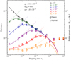 |
Fig. 4 Pebble accretion efficiency vs dimensionless stopping time for several values of the vertical turbulence strength, parameterized by αz (colors). Open symbols give ϵ obtained from directly integrating the stochastic equation of motion, while crosses give the results from the hybrid algorithm. Crosses are offset by 20% to the right for clarity. Error bars correspond to the Poisson counting error on the number of hits. For αz = 0 the triangles give ε resulting from the local calculations and the black line gives our fit to the 2D limit (ϵ2D), which we obtained in Paper I. The dotted lines gives ϵ3D accounting just for the density correction Eq. (22). The colored solid lines give ε accounting for all 3D/2D-effects (Eq. (40)) as explained in the main text. The right y-axis converts ε into the pebble growth mass – the total amount of pebbles needed to e-fold the mass of the planet – assuming a solar-mass star. |
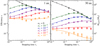 |
Fig. 5 Efficiency of pebble accretion of a 0.01 M⊕ planet (qp = 3 × 10⁻⁸) at 1 au (left panel) and at 30 au (right panel). At 1 au hgas = 0.03 and η = 10−3, while at 30 au we take hgas = 0.07 and η = 5 × 10⁻³. Right axis gives the planet growth mass. At 30 au turbulence more significantly affects the pebble accretion efficiency. |
4.3 Efficiency at H2O iceline for different stellar mass
There have been a number of studies that argue for the H2O iceline as a preferential site for the formation of the (first) generation of planetesimals and planetary embryos (Cuzzi & Zahnle 2004; Ros & Johansen 2013; Banzatti et al. 2015; Ida & Guillot 2016; Schoonenberg & Ormel 2017; Dra̧żkowska & Alibert 2017). In many of these works, the abundance of ices increases just outside the iceline by condensation of H2O vapor that diffused back over the iceline. In addition the surface density increases through a “traffic jam” effect when evaporating ice boulders liberate much smaller grains. For these reasons it is worthwhile to consider the efficiency of pebble accretion at the snowline. However, the snowline locations vary with stellar mass. In disks of lower mass stars the snowline will be much closer in, where the disk aspect ratio is likely to be smaller.
In Fig. 6 the pebble accretion efficiency is plotted at the H2O iceline, contrasting a solar type star (bottom) with a late M-star (top). The planet mass is 0.1 M⊕ in both cases. Two effects conspire to render efficiencies much higher for icelines around low-mass stars. First, the aspect ratio and η are lower because the iceline lies further in. Second, a planet(esimal) of the same mass around a lower mass star will have a higher mass ratio (qp). The pebble accretion cross section is then larger because of the reduced Keplerian shear and headwind velocities. Figure 6b illustrates the effect for a 0.1 M⊙ M-star for (the same) 0.1 M⊕ mass planet with hgas = 0.03 and η = 10−3; i.e., qp is higher by a factor of 10, hgas lower by a factor of 1.6, and η lower by a factor 3 compared to the solar-type star. Clearly, M-star pebble accretion efficiencies are both higher and are less sensitive to variations inτs and αz. Therefore, (late type) M-stars can efficiently convert their pebble-sized building blocks into planetary systems. These finding confirm our earlier analytical estimates on a pebble formation origin of the TRAPPIST-1 system (Ormel et al. 2017).
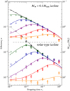 |
Fig. 6 Pebble accretion efficiency for a 0.1 M⊕ planet at thelocation of the H2O iceline. Top panel: iceline around a 0.1 M⋆ mass star (hgas = 0.03, η = 10−3; qp = 3 × 10⁻⁶). Bottom panel: iceline of a solar mass star (hgas = 0.05, η = 3 × 10⁻³, and qp = 3 × 10⁻⁷). |
4.4 Dichotomy of the solar system
It was argued by Morbidelli et al. (2015) that pebble accretion is more efficient beyond the H2O iceline because icy pebbles, being less prone to collisional fragmentation, are larger (higher τs). Specifically, Morbidelli et al. (2015) adopted τs = 10−1.5 for icy pebbles outside the iceline and τs = 10−2.5 for silicate pebbles (just) interior to the iceline and adopted αz = 10−3. The curve corresponding to these parameters is the purple curve in the bottom panel of Fig. 6. The positive slope indeed indicates that larger (icy) pebbles have a higher ε than the smaller (silicate) pebbles, a situation that generally applies to the 3D limit (Eq. (22)) where the pebble aspect ratio hP decreases with higher τs. Morbidelli et al. (2015) concluded that embryos just outside the H2O iceline will outcompete inner embryos8, arguing that the great dichotomy of the solar system – small Mars next to big Jupiter – is well explained under a pebble accretion scenario.
There is a corollary to this hypothesis, not (explicitly) addressed by Morbidelli et al. (2015). As Fig. 6 shows, the efficiencies of the τs = 10−1.5 pebbles (ε ≈ 0.4%) are very small: >99% of the pebbles drift past the planet to enrich the inner solar system. This means that the formation of Jupiter’s core is associated with hundreds of Earth masses in pebbles drifting into the terrestrial planet region. Evidently, in the scenario outlined by Morbidelli et al. (2015), most pebbles could not have been accreted by the bodies in the inner solar system but must have ended up in the young Sun. This puts a constraint on the structure of the inner disk, i.e., it had to be transparent to pebble drift. No dense planetesimals belts or long-lived pressure maxima (which could trigger formation of super-Earths; Chatterjee & Tan 2014) could have existed in the inner solar system during Jupiter’s formation.
4.5 Inclined planets
When planet(esimal)s move on orbits inclined with respect to the disk, the pebble accretion efficiency can be significantly reduced (Johansen et al. 2015; Levison et al. 2015). Planets of high inclination ip, such that ip > hP, only interact with pebbles overa fraction ~ip∕hP of their orbits. Inclined planets, therefore, have a similar effect on the settling efficiencies as turbulence: the higher the inclination, the less it interacts with the pebbles. In addition, inclined planets encounter pebbles at an additional velocity (~ ipvK), which suppresses accretion once it exceeds v*.
These effects are illustrated in Fig. 7, where ε is plotted as function of inclination ip (curves) for the laminar disk (αz = 0; all pebbles in the midplane), αz = 10−4, and αz = 10−2. In general, the higher the inclination, the lower the accretion efficiencies. For αz = 0 inclination effects already become visible for ip~10−3, whereas for αz = 10−2 the curves only diverge for ip > 10−2 (inclinations are given in radians). Accretion of large τs particles in particular are suppressed because of the increase in the approach velocity and the decrease in fset. The planet moves too fast through the pebble plane.
Since the planet’s inclination has a similar effect on ε as turbulent stirring of pebbles – both reduce the amount of interaction between the two-components – an effective scaleheight may be defined as heff ≃ ip + hP. A more precise estimate is obtained by averaging the pebble density over the phase of the planet’s orbit
 (25)
(25)
where  is the normal distribution with standard deviation hP and t the phase (mean anomaly). In the limit of ip ≪ hP,
  and heff is equal to the pebble scaleheight. More generally, the formal solution to Eq. (25) reads
![Mathematical equation: \begin{equation*} h_{\mathrm{eff}} = h_p \frac{\exp\left[ i_p^2/4h_P^2 \right]}{I_0(i_p^2/4h_P^2)},\end{equation*}](/articles/aa/full_html/2018/07/aa32562-17/aa32562-17-eq50.png) (26)
(26)
where I0(x) is the modified Bessel function of the first kind. For practical purposes, Eq. (26) may be approximated as
![Mathematical equation: \begin{equation*}h_{\mathrm{eff}} \approx \sqrt{h_P^2 +\frac{\pi i_p^2}{2} \left( 1-\exp\left[ -i_p/2h_P \right] \right)}. \end{equation*}](/articles/aa/full_html/2018/07/aa32562-17/aa32562-17-eq51.png) (27)
(27)
In the limit ip ≫ hP,  , implying that our first guess (heff = ip) is off by 25%. The reason is that the inclined planet spends most of its time near its end points, whereas it moves quickly through the midplane regions.
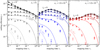 |
Fig. 7 Planet inclination dependence on pebble accretion efficiency. We plot ε for our standard parameters (qp = 3 × 10⁻⁷, η = 10−3 and hgas = 0.03) as function of τs (x-axis), αz (panels) and planet inclination ip (colors). Curves give our fit (Sect. 4.7). The plotted planet inclination values are ip = 0 (black, top), 10−3, 2 × 10⁻³, 5 × 10⁻³, 10−2, 2 × 10⁻², 5 × 10⁻² and 0.1 radians. Many of the low ip points and curves overlap. |
4.6 Role of turbulence – refinement of fset
We refine the expression for fset (Eq. (24)) accounting for a, possibly anisotropic, turbulent velocity field. Let Δ v be the non-turbulent component of the approach velocity with its component, Δ vi, pointing in the, ith direction. Concerning the planar direction, we already obtained Δv in Paper I, which we now relabel Δvy:
 (28)
(28)
where
 (29)
(29)
is the approach velocity in the circular limit. It combines the headwind (approach velocity dominated by ηvK) and the shear (approach velocity determined by the Keplerian shear velocity) regimes. In addition,
 (30)
(30)
is the eccentric velocity. In the above formulae, acir, ae and ash are all fit constants (see Table 1).
Similarly, for the vertical approach velocity, we have
 (31)
(31)
form the planet’s inclination. The order of unity prefactor ai is again obtained numerically.
We assume a tri-axial Gaussian velocity distribution of width σP, centered on Δv. Explicitly, for component i the approach velocity vi is normally distributed:
![Mathematical equation: \begin{equation*} P(v_i) = \frac{1}{\sigma_{\mathrm{P},i}\sqrt{2\pi}} \exp \left[ - \frac{(v_i -\mathrm{\Delta} v_i)^2}{2\sigma_{\mathrm{P},i}^2} \right],\vspace*{-2pt} \end{equation*}](/articles/aa/full_html/2018/07/aa32562-17/aa32562-17-eq57.png) (32)
(32)
where σP,i is the turbulent rms velocity in direction i. Following Youdin & Lithwick (2007), we take
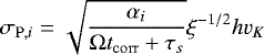 (33)
(33)
for the pebble rms velocity where ξ is defined in Eq. (16). From Eq. (24), we can write for the accretion probability
![Mathematical equation: \begin{equation*}f_{\mathrm{acc}} = \exp\left[-a_{\mathrm{set}} \frac{v_x^2 +v_y^2 +v_z^2}{v_{\ast}^2} \right].\vspace*{-2pt} \end{equation*}](/articles/aa/full_html/2018/07/aa32562-17/aa32562-17-eq59.png) (34)
(34)
The new, distribution-averaged fset is then obtained, by integration over the velocity distribution:
![Mathematical equation: \begin{align*}&f_{\mathrm{set}} = \int f_{\mathrm{acc}} P(v_x) P(v_y) P(v_z) \mathrm{d}v_x \mathrm{d}v_y \mathrm{d} v_z \nonumber\\ & \quad\quad\quad= \prod_i \exp \left[ -a_{\mathrm{set}} \frac{\mathrm{\Delta} v_i^2}{v_{\ast}^2 +a_{\mathrm{turb}}\sigma_{\mathrm{P},i}^2} \right] \frac{v_{\ast}}{\sqrt{(v_{\ast}^2 +a_{\mathrm{turb}}\sigma_{\mathrm{P},i}^2)}}.\vspace*{-2pt} \end{align*}](/articles/aa/full_html/2018/07/aa32562-17/aa32562-17-eq60.png) (35)
(35)
Formally, the integration gives aturb = 2aset, but we relax this constant in order to obtain the best fit to the simulated data.
Equation (35) features the following limits:
- 1.
σP,x, σP,y, σP,z ≪ v*. Turbulence is unimportant and the laminar form of fset is retrieved, Eq. (24).
- 2.
Isotropic turbulence, σP,x = σP,y = σP,z = σP. This simplifies Eq. (35) to
![Mathematical equation: \begin{equation*}f_{\mathrm{set}} = \exp \left[ -a_{\mathrm{set}} \frac{\mathrm{\Delta} v^2}{v_{\ast}^2 +a_{\mathrm{turb}}\sigma_P^2} \right] \frac{v_{\ast}^3}{(v_{\ast}^2 +a_{\mathrm{turb}}\sigma_P^2)^{3/2}}.\vspace*{-2pt}\end{equation*}](/articles/aa/full_html/2018/07/aa32562-17/aa32562-17-eq61.png) (36)
(36) - 3.
σP,x = σP,y = 0 with turbulence only operating in the vertical direction, which is (by construction) the case considered in this paper and may be applicable to the vertical shear instability (Stoll et al. 2017). Hence, we have used here
![Mathematical equation: \begin{equation*} f_{\mathrm{set}} = \exp\left[ -a_{\mathrm{set}} \left( \frac{\mathrm{\Delta} v_y^2}{v_{\ast}^2} +\frac{\mathrm{\Delta} v_z^2}{v_{\ast}^2 +a_{\mathrm{turb}}\sigma_{\mathrm{P},z}^2} \right) \right] \frac{v_{\ast}}{\sqrt{v_{\ast}^2 +a_{\mathrm{turb}}\sigma_{\mathrm{P},z}^2}}.\vspace*{-2pt} \end{equation*}](/articles/aa/full_html/2018/07/aa32562-17/aa32562-17-eq62.png) (37)
(37) - 4.
σP,x ≃ σP,y ≃ σP,z ≃ σP ≫ v* + Δv, the turbulence-dominant limit. In this case
 (38)
(38)Turbulence reduces the accretion, but not exponentially. In a turbulence-dominated velocity field there is always a fraction of particles with velocities low enough to accrete by settling.
Breakdown of the expressions and parameters involved in the pebble accretion efficiency.
4.7 Summary of the pebble accretion efficiency fit
We provide an executive summary on how to generally obtain ε. Quantities involving the recipe and corresponding numerical constants are given in Table 1.
The settling efficiencies in the 2D and 3D limits read
 (39a)
(39a)
 (39b)
(39b)
Apart from the fset term, the 3D expression is independent of the pebble-planet relative velocity; a characteristic feature of pebble accretion in the 3D limit (Ormel 2017; Paper I). The effective scaleheight, heff, Eq. (27), accounts for the reduced interaction between pebble and planetesimal by either turbulent stirring of pebbles or planetesimal inclination. The non-turbulent component of the relative motion Δ v is given by Eqs. (28) and (31), for the azimuthal and vertical component respectively.
The other velocity-dependent term is the settling fraction fset, which becomes important when either laminar or turbulent velocities exceed the critical settling velocity  . In the laminar case (σ = 0) fset is given by Eq. (24), while in the turbulent case (σ≠0) it is given by Eq. (35). When v* significantly exceeds σ + Δv the settling fraction evaluates to unity.
Finally, we find that the 3D (this Paper) and 2D (Paper I) can be combined as
 (40)
(40)
which ensures a smooth transition. All curves shown in Figs. 4–9 follow this recipe.
When fset ≪ 1 (e.g., Δv ≫ v* or σ ≫ v*) the ballistic regime (see Paper I) takes over. In Paper I we found that the combined efficiency is well-fitted by
 (41)
(41)
where εbal is the efficiency in the ballistic limit (see Paper I). However, in 3D growth by ballistic encounters is generally slow.
4.8 Neglected effects
We list several neglected effects, which may change ε:
- 1.
Aerodynamical deflection. For planetesimals, we have not accounted for the change in vgas in the vicinity of the planetesimals and correspondingly ignored aerodynamic deflection (Visser & Ormel 2016). This reduction, however, only becomes important when particles are very small, tstop < R∕vhw, and only when the encounters operate in the ballistic regime. Under these conditions, turbulence may in fact overcome the aerodynamic barrier (Homann et al. 2016).
- 2.
Pre-planetary atmospheres. We have not accounted for the effects of the early primordial atmosphere that forms around massive bodies in gaseous disks. As a rule of thumb, this affects the density and flow pattern out to a Bondi radius,
 . Planets as massive as the thermal mass (h3M⋆) will have such extensive envelopes that our constant-density assumption will break down. A complex flow structure may prevent small particles from accreting to the planet (Ormel 2013), perhaps after their evaporation (Chambers 2017; Brouwers et al. 2018).
 - 3.
Pressure maxima and resonances. Such massive planets also affect the pressure profile of the disk, resulting in a pressure maximum at a distance ~Hgas from the planet. For this pebble isolation mass, accretion will terminate (Lambrechts et al. 2014; Bitsch et al. 2018b). Similarly, τs > 1 pebbles can be stopped at resonant location (Weidenschilling & Davis 1985; Picogna et al. 2018).
- 4.
Gas radial flow. In viscous disks, gas flows radial at a velocity ~− ν∕r and adds to the drift velocity of pebbles. This effect hence starts to dominate radial drift motions for αν > τs. It is straightforward to adjust expressions for ε (see, e.g., Ida et al. 2016). Similarly, the drift velocity depends on vertical position, vr(z), because τs increases towards the disk surface. We can correct ε accordingly, i.e., by using a vertically averaged vr (Takeuchi & Lin 2002; Kanagawa et al. 2017).
- 5.
By design, the simulations of this work only considered turbulence in the vertical direction – a simplification that allowed us to carry out a numerical parameter study in a controlled way. By modeling vertical turbulence we have accounted for the reduction of the midplane pebble density. On the other hand, the reduction of ε by fast encounters is underestimated in the numerical simulations, particularly when the turbulence is strongly anisotropic (σx, σy ≫ σz). Nevertheless, in Sect. 4.6 we formulated a general recipe for fset in a anisotropic velocity field.
5 Discussion
Table 2 compiles expressions for ε that have been used in, or derived from, recent studies. For simplicity, we ignore the fset term and list the numerical prefactor belonging to the leading term for the 3D and the 2D limits. In the 2D limit the shear-dominated velocity regime has been adopted (valid for large planets), while in the 3D limit the expression is independent of Δ v. We emphasize that this work gives the correct numerical prefactor, as it is calibrated against numerical simulations. On the other hand, the existing literature expressions often employed scaling arguments, where typically the 3D rate is estimated to be a fraction bset ∕HP of the 2D rate where bset is the pebble accretion impact parameter. It is therefore quite remarkable that the existing literature prefactors lie so close to our calculated values. Nevertheless, in the 2D-limit the literature expression turn out to be too high, up to 50%. This may still be significant, since a factor of two difference means that planet formation by pebble accretion takes twice as long and requires twice the number of pebbles.
Like our study, Chambers (2014) considered the cases where planet eccentricity (inclinations) dominate and accounts for the velocity effect of turbulence. However, he only considered the turbulent rms velocity for the relative motion between planet and pebble, which suppresses pebble accretion exponentially (fset ≫ 1) once σ ≫ v*. This is illustrated in Fig. 8 by the gray curve, where the settling fraction is plotted as function of planet mass. Parameters are chosen such that turbulent rms velocities  are similar to the laminar headwind velocity, ηvK. When fset is calculated by adding in quadrature the laminar and turbulent rms velocities (as in Eq. (24)), it ensures exponential behavior at low qp. However, accounting for a velocity distribution changes the functional behavior of fset and, for the adopted parameters, we obtain the counter intuitive result that turbulence increases fset (at low qp; solid curve). Accounting for the distribution, there are always a few particles slow enough for the settling mechanism to operate. This finding is important especially in the outer disk, where even at fset ~10−3 settling interactions dominate over ballistic interactions.
Recently, Xu et al. (2017) measured pebble accretion rates from laminar and MRI-turbulent hydrodynamical simulations. They expressed their result in terms of a dimensionless quantity kabs, which is the ratio of the mass accretion rate (Ṁ) normalized to the Hill accretion rate  . In these units, our expressions for the 2D and 3D efficiencies (Eq. (39)) read9:
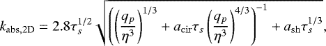 (42a)
(42a)
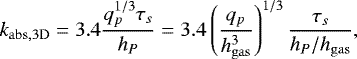 (42b)
(42b)
where we did insert Δv in Eq. (42a), but have for clarity omitted the fset modulation factor.
As a note in passing, Eq. (42a) depends, apart from τs, only on the quantity qp∕η3. The reason is that the pebble equation of motion, expressed in Hill units, only contains this parameter10. Likewise, the 3D-rates also depend on a single, but different, parameter (assuming heff can be quantified in terms of the stopping time). In the general case, then, two parameters (or three if τs is included) are necessary to calculate the Hill accretion rate. In their local shearing box simulations, Xu et al. (2017) choose to fix the thermal mass  and the quantity η∕hgas. For the Hill accretion rate (kabs), the problem is then fully specified. However, to calculate the efficiencies (ε) the degeneracy that existed among qp, η, and hgas is broken – qp, η, and hgas each need to be specified. This is because the accretion rate is a local quantity, whereas in order to calculate ε the radial pebble flux must be known, i.e., the disk circumference should be specified.
In Fig. 9 symbols correspond to the runs conducted by Xu et al. (2017, their Fig. 4a) for a thermal mass of  and a headwind parameter of η = 0.1hgas. Blue symbols correspond to the hydrodynamic runs (non-turbulent), green symbols to the ambipolar diffusion runs, and red symbols to the ideal MRI runs. As expected, the accretion rate decreases in the turbulent case and more so in the ideal MRI run than in the AD-restive run. Solid curves give the corresponding kabs obtained from Eq. (42), fset, and the 2D and 3D averaging formula (Eq. (40))11. Fits are plotted until τs = 1 beyond which they loose their validity.
The results of our analytical model agree well with Xu et al. (2017). For the turbulent runs, we find that the reduction of the accretion rate is mostly due to turbulent diffusion (turbulence lofting pebbles away from the midplane) rather than the turbulent velocity effect. This explains why the ideal MRI run features lower accretion rates than the ambipolar diffusion runs. Towards τs = 0.1–1 we see that the ambipolar diffusion run and the hydrodynamic run converge, as the accretion becomes 2D and turbulent diffusion does not enter kabs. However, we also find that the ideal MRI run does not entirely converge on the hydrodynamic run. This can be attributed to the turbulent velocity effect; fset ≲ 1 because σ ≳ v* for the τs ≃ 0.1–1 particles in the MRI run. In other words, settling is marginally failing. We anticipate a much stronger reduction for either smaller planets or more vigorous turbulence.
Collected efficiency expressions used in recent studies.
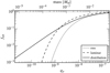 |
Fig. 8 Settling fraction fset as function of planet mass for αz = 10−2, hgas = 0.05, η = 5 × 10⁻³, τs = 0.1 and M⋆ = 1 M⊙. Turbulence is assumed to be isotropic and the correlation time tcorr = Ω−1. Curves give fset when it is calculated based on the laminar-only velocity (dashed), turbulent rms velocity (gray), and for a distribution of velocities (solid). |
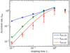 |
Fig. 9 Hill-normalized accretion rates for a planet of thermal mass |

6 Summary
In this work we have developed a general framework for the stochastic equation of motion (SEOM) of pebble-sizedparticles. The SEOM is described by the particle’s stopping time, by the gas diffusivity Dgas and correlation time tcorr, and by gravitational forces. Using the SEOM we have investigated the vertical transport of particles in disks.
- 1.
From the SEOM we obtain the strong coupling approximation (SCA) by taking the limit of tstop → 0, as was used in previous studies (Ciesla 2010; Zsom et al. 2011). For small tstop and tcorr the SEOM becomes consistent with the SCA.
- 2.
Exploring the effect of a vertically dependent diffusivity, αz(z), such that the midplane diffusivity αmid ≪ τs and the surface diffusivity αsurface ≫ τs, we find a two component distribution for the pebbles. Although most of the pebbles are concentrated in the midplane (following the scaleheight given by αmid), a small fraction of pebbles are distributed according to the gas scaleheight. Then, high-velocity collisions among these pebbles could explain the prolonged presence of small, micron-sized grains in the disk surface.
As its main application, we have integrated pebble trajectories to find the pebble accretion efficiency ε.
- 1.
Compared to the laminar disk, turbulence reduces ε in two ways: it diminishes the local density of pebbles at the midplane through diffusion and it increases the rms velocity of particles. The latter becomes important for low planet masses, where fulfilling the settling condition becomes more difficult.
- 2.
Because of the disk geometry, pebble accretion is more efficient in the inner disk. From an efficiency perspective, accretion around low-mass stars is also favored because pebble capture radii are larger around low-mass stars.
- 3.
Together with the 2D expressions already derived in Paper I, we have formulated a general prescription for ε as a function of pebble properties (aerodynamical size), planet properties (mass, inclination, eccentricity), and disk properties (pressure profile, gas density, turbulence properties). This prescription is summarized in Sect. 4.7.
Finally, we remark that ε has been defined with respect to a single planet. A small ε therefore does not necessarily imply that pebble accretion is globally inefficient. Indeed, in the case of a planetesimal belt (or multiple planets), the total filtering efficiency may well reach unity, whereas the individual ε ≪1 (Guillot et al. 2014). This raises the question of how pebble accretion proceeds when multiple seeds are present.
While it is likely to result in a more efficient pebble sweep-up, a multi-seed scenario could also suppress planet growth because of the mutual dynamical excitation among the protoplanets (Levison et al. 2015). In a following work, we will investigate the efficacy of pebble accretion when pebbles interact with a narrow planetesimal belt (Liu et al., in prep.). In such cases, the combined planetesimal and pebble coagulation can best be studied with N-body techniques, where the pebble accretion rate on the N-bodies is obtained using the prescription for ε summarized in Sect. 4.7.
Acknowledgements
The authors are supported by the Netherlands Organization for Scientific Research (NWO; VIDI project 639.042.422). We thank Xuening Bai and Ziyan Xu for sharing and discussing their simulations, and Ramon Brasser and Sebastiaan Krijt for proofreading the manuscript. The comments from the referee improved the clarity of the manuscript.
Appendix A Proof of Equation (10)
In deriving Eq. (10), we follow the proof outlined by Hottovy et al. (2015). The first step is to write Eq. (4) as
 (A.1a)
 (A.1b)
In this equation, the stochastic variable ζt has been combined with the velocity into one vector v = (v, ζt). Similarly, x contains an additional parameter, say υ, but this is entirely dummy. Comparing with Eq. (4), we therefore have
 (A.2a)
 (A.2b)
 (A.2c)
It must be emphasized that we only treat here the z coordinate. When the full 3D equation of motion is considered, v will be vector of length six and γ a matrix of 36 elements, containing all entries of the diffusion tensor Dij.
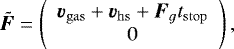
In the limit of tstop → 0, Hottovy et al. (2015) proves that x can be described by the SDE
![Mathematical equation: \begin{equation*}\bm{x} = \left[ \boldsymbol{\upgamma}^{-1} \bm{\tilde{F}} +\bm{S} \right] \mathrm{d} t +\boldsymbol{\upgamma}^{-1}\bm{\sigma} d\bm{W}_t,\vspace*{-3pt} \end{equation*}](/articles/aa/full_html/2018/07/aa32562-17/aa32562-17-eq81.png) (A.3)
(A.3)
where γ−1 is the inverse of γ and S is the noise-induced drift term – a vector whose ith component is defined
![Mathematical equation: \begin{equation*} \bm{S}_i = \sum_{j,l} \frac{\partial}{\partial x_l} \left[ (\boldsymbol{\upgamma}^{-1})_{ij} \right] \mathbf{J}_{jl}\vspace*{-3pt} \end{equation*}](/articles/aa/full_html/2018/07/aa32562-17/aa32562-17-eq82.png) (A.4)
(A.4)
with J the solution of the Lyapunov equation
 (A.5)
(A.5)
Since we consider here only the z coordinate, Eq. (A.3) reduces too
 (A.6)
(A.6)
The equations can now be solved. Inverting γ we find
 (A.7)
(A.7)
Furthermore, solving the Lyapunov equation, we find
 (A.8)
(A.8)
with which the noise-induced drift term becomes
 (A.9)
(A.9)
and we retrieve Eq. (10).
A.1 Stratonovich interpretation
A feature peculiar to stochastic integrals is that equations of the form
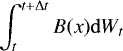 (A.10)
are ill-defined when B is a function of position. In contrast to ODEs, it does matter whether the integrand is evaluated at t (i.e., B(x) = B(x[t]) – Ito’s choice), at t + Δt, or whether we let
![Mathematical equation: \begin{equation*} \int_{t}^{\mathrm{\Delta} t} B(x) \mathrm{d} W_t \approx \frac{1}{2} B\left( \frac{x[t] +x[t+\mathrm{\Delta} t]}{2} \right) \left( W_{t+\mathrm{\Delta} t} -W_t \right) \end{equation*}](/articles/aa/full_html/2018/07/aa32562-17/aa32562-17-eq89.png) (A.11)
(A.11)
(Stratonovich’ choice). These definitions will produce different results when B is not constant (van Kampen 1992). Specifically, with Stratonovich’, rather than Ito’s, interpretation for the stochastic integral, a term
 (A.12)
should be added to the RHS of the Fokker–Planck Eq. (12).
In deriving Eq. (10), as well as the conversion from Eq. (10) to Eq. (13), we have followed Ito’s interpretation. On the other hand, under Stratonovich interpretation, the RHS of Eq. (10) and the RHS of Eq. (13) gain an additional term  :
:
 (A.13)
Hence, the SDE for the strong coupling approximation depends on the interpretation rule (a fact not highlighted by Ciesla 2010 or Zsom et al. 2011). The underlying reason between the Ito and Stratonovich interpretations reflects the nature of the stochastic forcing (van Kampen 1992). Ito’s interpretation would hold, for example, when the stochastic forcing amounts to a series of infinitely short “pulses” with every pulse completely independent. This interpretation is often used in finance. However, it may be argued that for physical problems, where the correlation time is never really infinitely small, Stratonovich amounts to the more correct model (van Kampen 1992).
More practically, these differences are expressed in our choice of the numerical integration scheme. When Ito’s interpretation is adopted, the stochastic equation must be integrated with a corresponding numerical scheme, of which the Euler method is the simplest example. Similarly, the Stratonovich equation should be integrated with an appropriate numerical scheme, where the midpoint scheme (Heun’s method) is the simplest example. In our code, where we use an Runge–Kutta method, which is a generalization of a midpoint scheme, we therefore adopt Eq. (A.13), instead of Eq. (10).
References
- Ansdell, M., Williams, J. P., Manara, C. F., et al. 2017, AJ, 153, 240 [NASA ADS] [CrossRef] [EDP Sciences] [Google Scholar]
- Bai, X.-N., & Stone, J. M. 2011, ApJ, 736, 144 [NASA ADS] [CrossRef] [Google Scholar]
- Bai, X.-N., Ye, J., Goodman, J., & Yuan, F. 2016, ApJ, 818, 152 [Google Scholar]
- Balbus, S. A., & Hawley, J. F. 1991, ApJ, 376, 214 [NASA ADS] [CrossRef] [Google Scholar]
- Banzatti, A., Pinilla, P., Ricci, L., et al. 2015, ApJ, 815, L15 [NASA ADS] [CrossRef] [Google Scholar]
- Birnstiel, T., Dullemond, C. P., & Brauer, F. 2010, A&A, 513, A79 [NASA ADS] [CrossRef] [EDP Sciences] [Google Scholar]
- Birnstiel, T., Ormel, C. W., & Dullemond, C. P. 2011, A&A, 525, A11 [NASA ADS] [CrossRef] [EDP Sciences] [Google Scholar]
- Bitsch, B., Lambrechts, M., & Johansen, A. 2015, A&A, 582, A112 [NASA ADS] [CrossRef] [EDP Sciences] [Google Scholar]
- Bitsch, B., Lambrechts, M., & Johansen, A. 2018a, A&A, 609, C2 [CrossRef] [EDP Sciences] [Google Scholar]
- Bitsch, B., Morbidelli, A., Johansen, A., et al. 2018b, A&A, 612, A30 [NASA ADS] [CrossRef] [EDP Sciences] [Google Scholar]
- Brouwers, M. G., Vazan, A., & Ormel, C. W. 2018, A&A, 611, A65 [NASA ADS] [CrossRef] [EDP Sciences] [Google Scholar]
- Carballido, A., Bai, X.-N., & Cuzzi, J. N. 2011, MNRAS, 415, 93 [NASA ADS] [CrossRef] [Google Scholar]
- Chambers, J. E. 2014, Icarus, 233, 83 [NASA ADS] [CrossRef] [Google Scholar]
- Chambers, J. 2017, ApJ, 849, 30 [NASA ADS] [CrossRef] [Google Scholar]
- Charnoz, S., Fouchet, L., Aleon, J., & Moreira, M. 2011, ApJ, 737, 33 [NASA ADS] [CrossRef] [Google Scholar]
- Chatterjee, S., & Tan, J. C. 2014, ApJ, 780, 53 [NASA ADS] [CrossRef] [Google Scholar]
- Ciesla, F. J. 2010, ApJ, 723, 514 [NASA ADS] [CrossRef] [Google Scholar]
- Cuzzi, J. N., & Zahnle, K. J. 2004, ApJ, 614, 490 [NASA ADS] [CrossRef] [Google Scholar]
- Cuzzi, J. N., Hogan, R. C., Paque, J. M., & Dobrovolskis, A. R. 2001, ApJ, 546, 496 [NASA ADS] [CrossRef] [Google Scholar]
- Dra̧żkowska, J., & Alibert, Y. 2017, A&A, 608, A92 [NASA ADS] [CrossRef] [EDP Sciences] [Google Scholar]
- Dubrulle, B., Morfill, G., & Sterzik, M. 1995, Icarus, 114, 237 [NASA ADS] [CrossRef] [Google Scholar]
- Dullemond, C. P., & Dominik, C. 2005, A&A, 434, 971 [NASA ADS] [CrossRef] [EDP Sciences] [Google Scholar]
- Flaherty, K. M., Hughes, A. M., Rosenfeld, K. A., et al. 2015, ApJ, 813, 99 [NASA ADS] [CrossRef] [Google Scholar]
- Flaherty, K. M., Hughes, A. M., Rose, S. C., et al. 2017, ApJ, 843, 150 [NASA ADS] [CrossRef] [Google Scholar]
- Flock, M., Fromang, S., Turner, N. J., & Benisty, M. 2017, ApJ, 835, 230 [NASA ADS] [CrossRef] [Google Scholar]
- Gammie, C. F. 1996, ApJ, 457, 355 [NASA ADS] [CrossRef] [Google Scholar]
- Gressel, O. 2017, J. Phys. Conf. Ser., 837, 012008 [CrossRef] [Google Scholar]
- Gressel, O., Nelson, R. P., & Turner, N. J. 2011, MNRAS, 415, 3291 [NASA ADS] [CrossRef] [Google Scholar]
- Gressel, O., Nelson, R. P., & Turner, N. J. 2012, MNRAS, 422, 1140 [NASA ADS] [CrossRef] [Google Scholar]
- Guillot, T., Ida, S., & Ormel, C. W. 2014, A&A, 572, A72 [NASA ADS] [CrossRef] [EDP Sciences] [Google Scholar]
- Guilloteau, S., Dutrey, A., Wakelam, V., et al. 2012, A&A, 548, A70 [NASA ADS] [CrossRef] [EDP Sciences] [Google Scholar]
- Homann, H., Guillot, T., Bec, J., et al. 2016, A&A, 589, A129 [NASA ADS] [CrossRef] [EDP Sciences] [Google Scholar]
- Hottovy, S., McDaniel, A., Volpe, G., & Wehr, J. 2015, Commun. Math. Phys., 336, 1259 [NASA ADS] [CrossRef] [Google Scholar]
- Hughes, A. M., Wilner, D. J., Andrews, S. M., Qi, C., & Hogerheijde, M. R. 2011, ApJ, 727, 85 [NASA ADS] [CrossRef] [Google Scholar]
- Ida, S., & Guillot, T. 2016, A&A, 596, L3 [Google Scholar]
- Ida, S., Guillot, T., & Morbidelli, A. 2008, ApJ, 686, 1292 [NASA ADS] [CrossRef] [Google Scholar]
- Ida, S., Guillot, T., & Morbidelli, A. 2016, A&A, 591, A72 [NASA ADS] [CrossRef] [EDP Sciences] [Google Scholar]
- Johansen, A., & Lambrechts, M. 2017, Annu. Rev. Earth Planet. Sci., 45, 359 [Google Scholar]
- Johansen, A., Klahr, H., & Mee, A. J. 2006, MNRAS, 370, L71 [NASA ADS] [Google Scholar]
- Johansen, A., Mac Low, M.-M., Lacerda, P., & Bizzarro, M. 2015, Sci. Adv., 1, 15109 [Google Scholar]
- Juhász, A., Bouwman, J., Henning, T., et al. 2010, ApJ, 721, 431 [NASA ADS] [CrossRef] [Google Scholar]
- Kanagawa, K. D., Ueda, T., Muto, T., & Okuzumi, S. 2017, ApJ, 844, 142 [NASA ADS] [CrossRef] [Google Scholar]
- Kobayashi, H., Tanaka, H., Krivov, A. V., & Inaba, S. 2010, Icarus, 209, 836 [NASA ADS] [CrossRef] [Google Scholar]
- Kobayashi, H., Tanaka, H., & Okuzumi, S. 2016, ApJ, 817, 105 [NASA ADS] [CrossRef] [Google Scholar]
- Krijt, S., & Ciesla, F. J. 2016, ApJ, 822, 111 [NASA ADS] [CrossRef] [Google Scholar]
- Lambrechts, M., & Johansen, A. 2012, A&A, 544, A32 [Google Scholar]
- Lambrechts, M., & Johansen, A. 2014, A&A, 572, A107 [NASA ADS] [CrossRef] [EDP Sciences] [Google Scholar]
- Lambrechts, M., Johansen, A., & Morbidelli, A. 2014, A&A, 572, A35 [NASA ADS] [CrossRef] [EDP Sciences] [Google Scholar]
- Levison, H. F., Kretke, K. A., & Duncan, M. J. 2015, Nature, 524, 322 [CrossRef] [Google Scholar]
- Liu, B., & Ormel, C. W. 2018, A&A, 615, A138 (Paper I) [NASA ADS] [CrossRef] [EDP Sciences] [Google Scholar]
- Miotello, A., van Dishoeck, E. F., Williams, J. P., et al. 2017, A&A, 599, A113 [NASA ADS] [CrossRef] [EDP Sciences] [Google Scholar]
- Morbidelli, A., Lambrechts, M., Jacobson, S., & Bitsch, B. 2015, Icarus, 258, 418 [NASA ADS] [CrossRef] [Google Scholar]
- Nakagawa, Y., Sekiya, M., & Hayashi, C. 1986, Icarus, 67, 375 [NASA ADS] [CrossRef] [Google Scholar]
- Nelson, R. P., & Gressel, O. 2010, MNRAS, 409, 639 [NASA ADS] [CrossRef] [Google Scholar]
- Nelson, R. P., Gressel, O., & Umurhan, O. M. 2013, MNRAS, 435, 2610 [NASA ADS] [CrossRef] [Google Scholar]
- Okuzumi, S., & Ormel, C. W. 2013, ApJ, 771, 43 [NASA ADS] [CrossRef] [Google Scholar]
- Ormel, C. W. 2013, MNRAS, 428, 3526 [NASA ADS] [CrossRef] [Google Scholar]
- Ormel, C. W. 2017, in Astrophysics and Space Science Library, eds. M. Pessah & O. Gressel, 445, 197 [Google Scholar]
- Ormel, C. W., & Cuzzi, J. N. 2007, A&A, 466, 413 [NASA ADS] [CrossRef] [EDP Sciences] [Google Scholar]
- Ormel, C. W., & Klahr, H. H. 2010, A&A, 520, A43 [NASA ADS] [CrossRef] [EDP Sciences] [Google Scholar]
- Ormel, C. W., & Okuzumi, S. 2013, ApJ, 771, 44 [NASA ADS] [CrossRef] [Google Scholar]
- Ormel, C. W., Liu, B., & Schoonenberg, D. 2017, A&A, 604, A1 [NASA ADS] [CrossRef] [EDP Sciences] [Google Scholar]
- Paardekooper,S.-J., Rein, H., & Kley, W. 2013, MNRAS, 434, 3018 [NASA ADS] [CrossRef] [Google Scholar]
- Pan, L., & Padoan, P. 2010, J. Fluid Mech., 661, 73 [NASA ADS] [CrossRef] [Google Scholar]
- Picogna, G., Stoll, M. H. R., & Kley, W. 2018, A&A, in press, DOI:10.1051/0004-6361/201732523 [Google Scholar]
- Pinilla, P., Birnstiel, T., Ricci, L., et al. 2012, A&A, 538, A114 [NASA ADS] [CrossRef] [EDP Sciences] [Google Scholar]
- Pinte, C., Dent, W. R. F., Ménard, F., et al. 2016, ApJ, 816, 25 [NASA ADS] [CrossRef] [Google Scholar]
- Pollack, J. B., Hubickyj, O., Bodenheimer, P., et al. 1996, Icarus, 124, 62 [NASA ADS] [CrossRef] [Google Scholar]
- Rein, H., & Papaloizou, J. C. B. 2009, A&A, 497, 595 [NASA ADS] [CrossRef] [EDP Sciences] [Google Scholar]
- Ros, K., & Johansen, A. 2013, A&A, 552, A137 [NASA ADS] [CrossRef] [EDP Sciences] [Google Scholar]
- Safronov, V. S. 1969, in Evolution of the Protoplanetary Cloud and Formation of Earth and the Planets, ed. V. S. Safronov (Moscow: Nauka. Transl. 1972 NASA Tech. F-677) [Google Scholar]
- Sano, T., Inutsuka, S.-i., Turner, N. J., & Stone, J. M. 2004, ApJ, 605, 321 [NASA ADS] [CrossRef] [Google Scholar]
- Schoonenberg, D., & Ormel, C. W. 2017, A&A, 602, A21 [NASA ADS] [CrossRef] [EDP Sciences] [Google Scholar]
- Shakura, N. I., & Sunyaev, R. A. 1973, A&A, 24, 337 [NASA ADS] [Google Scholar]
- Smoluchowski, M. V. 1916, Z. Phys., 17, 557 [NASA ADS] [Google Scholar]
- Stoll, M. H. R., & Kley, W. 2014, A&A, 572, A77 [NASA ADS] [CrossRef] [EDP Sciences] [Google Scholar]
- Stoll, M. H. R., Kley, W., & Picogna, G. 2017, A&A, 599, L6 [NASA ADS] [CrossRef] [EDP Sciences] [Google Scholar]
- Suzuki, T. K., Ogihara, M., Morbidelli, A., Crida, A., & Guillot, T. 2016, A&A, 596, A74 [NASA ADS] [CrossRef] [EDP Sciences] [Google Scholar]
- Takeuchi, T., & Lin, D. N. C. 2002, ApJ, 581, 1344 [NASA ADS] [CrossRef] [Google Scholar]
- Tanaka, H., Himeno, Y., & Ida, S. 2005, ApJ, 625, 414 [NASA ADS] [CrossRef] [Google Scholar]
- Teague, R., Guilloteau, S., Semenov, D., et al. 2016, A&A, 592, A49 [NASA ADS] [CrossRef] [EDP Sciences] [Google Scholar]
- Uhlenbeck, G. E., & Ornstein, L. S. 1930, Phys. Rev., 36, 823 [NASA ADS] [CrossRef] [Google Scholar]
- van Kampen, N. G. 1992, Stochastic Processes in Physics and Chemistry (Amsterdam, The Netherlands: Elsevier) [Google Scholar]
- Visser, R. G., & Ormel, C. W. 2016, A&A, 586, A66 [NASA ADS] [CrossRef] [EDP Sciences] [Google Scholar]
- Völk, H. J., Jones, F. C., Morfill, G. E., & Roeser, S. 1980, A&A, 85, 316 [NASA ADS] [Google Scholar]
- Weidenschilling, S. J. 1977, MNRAS, 180, 57 [NASA ADS] [CrossRef] [Google Scholar]
- Weidenschilling, S. J., & Davis, D. R. 1985, Icarus, 62, 16 [NASA ADS] [CrossRef] [Google Scholar]
- Xu, Z., Bai, X.-N., & Murray-Clay, R. A. 2017, ApJ, 847, 52 [NASA ADS] [CrossRef] [Google Scholar]
- Youdin, A. N., & Lithwick, Y. 2007, Icarus, 192, 588 [NASA ADS] [CrossRef] [Google Scholar]
- Zhu, Z., Stone, J. M., & Bai, X.-N. 2015, ApJ, 801, 81 [NASA ADS] [CrossRef] [Google Scholar]
- Zsom, A., Ormel, C. W., Dullemond, C. P., & Henning, T. 2011, A&A, 534, A73 [NASA ADS] [CrossRef] [EDP Sciences] [Google Scholar]
The standard assumption is that αz relates to the turbulent velocity as in  with cs the isothermal sound speed, but this identification assumes that the correlation time tcorr = Ω−1. See discussion in Sect. 2.3.
In Guillot et al. (2014) and Lambrechts & Johansen (2014) a similar quantity is defined.
In Eq. (3) and other equations, the differential operator ∂∕∂z is understood to act on both terms to its right.
The Youdin & Lithwick (2007) study pertains to non-stratified disks. Equation (15) was suggested to account for stratification effects.
We calculate Δrsynfrom the equation
 (19) where vr and vϕ are the radial and azimuthal drift velocities (e.g., Weidenschilling 1977). Approximating the integral to second order in Δ rsyn, we obtain
 (20) where
 .
.
The magnitude of the unperturbed relative velocity between planet and pebble.
Apart from a higher ε another reason is that the icy pebble flux is larger than the silicate pebble flux, due to evaporation of H2O.
See Ormel & Klahr (2010), where the parameter, denoted ζw, is expressed as the ratio of the Hill velocity to the disk headwind,  .
.
In evaluating the expressions, we used the turbulent diffusivities reported by Xu et al. (2017): αz = 7.8 × 10⁻⁴ (ambipolar diffusion) and αz = 4.4 × 10⁻³ (ideal MRI). Similarly, we use the (midplane) rms gas velocities from these simulations (Ziyan Xu, priv. comm.).
All Tables
Breakdown of the expressions and parameters involved in the pebble accretion efficiency.
All Figures
|
Fig. 1 Top panel: normalized distributions of the vertical position z for the integration of the tracer case, using the strong coupling approximation (SCA) with tstop = 0. The vertical height z is recorded after every 1 Ω−1 for t = 105 Ω−1. Bars give the simulated distribution while the analytic – normal – distribution is shown by the black dashed line. Bottom panel: temporal evolution of the vertical position for αz = 10−2 (black) and αz = 10−2 (blue). |
| In the text | |
|
Fig. 2 Vertical distribution for particles of different stopping times: τs = tstopΩ = 10−2 (panel a), 10−1 (panel b), and 1 (panel c). Histograms plot the numerically obtained distributions with the stochastic equation of motion (SEOM; gray and red) and strong coupling approximation (SCA; blue) methods. Long tcorr runs are shown with red histograms (the tcorr = 102 Ω−1, τs = 0.1 run is displayed in panel c). Thin curves gives the normal distribution with the scaleheight of Eq. (15) (Youdin & Lithwick 2007). Note the different scaling among the panels. |
| In the text | |
|
Fig. 3 Density distribution P(z) obtainedfrom a vertically varying diffusivity. The diffusivity profile in terms of αz is given by the red curve. The particle stopping time is τs = 10−2 and is taken independent of z. The distributions obtained from integrating the stochastic equation of motions (Eq. (4); black histogram) and the strong coupling approximation (Eq. (10); gray histograms) are consistent. The dark blue curve gives the normal distribution, for the particle scaleheight evaluated in the midplane (i.e., Eq. (15) with α = 10−3). The light blue curves gives the gas distribution, scaled by a factor 0.1. |
| In the text | |
|
Fig. 4 Pebble accretion efficiency vs dimensionless stopping time for several values of the vertical turbulence strength, parameterized by αz (colors). Open symbols give ϵ obtained from directly integrating the stochastic equation of motion, while crosses give the results from the hybrid algorithm. Crosses are offset by 20% to the right for clarity. Error bars correspond to the Poisson counting error on the number of hits. For αz = 0 the triangles give ε resulting from the local calculations and the black line gives our fit to the 2D limit (ϵ2D), which we obtained in Paper I. The dotted lines gives ϵ3D accounting just for the density correction Eq. (22). The colored solid lines give ε accounting for all 3D/2D-effects (Eq. (40)) as explained in the main text. The right y-axis converts ε into the pebble growth mass – the total amount of pebbles needed to e-fold the mass of the planet – assuming a solar-mass star. |
| In the text | |
|
Fig. 5 Efficiency of pebble accretion of a 0.01 M⊕ planet (qp = 3 × 10⁻⁸) at 1 au (left panel) and at 30 au (right panel). At 1 au hgas = 0.03 and η = 10−3, while at 30 au we take hgas = 0.07 and η = 5 × 10⁻³. Right axis gives the planet growth mass. At 30 au turbulence more significantly affects the pebble accretion efficiency. |
| In the text | |
|
Fig. 6 Pebble accretion efficiency for a 0.1 M⊕ planet at thelocation of the H2O iceline. Top panel: iceline around a 0.1 M⋆ mass star (hgas = 0.03, η = 10−3; qp = 3 × 10⁻⁶). Bottom panel: iceline of a solar mass star (hgas = 0.05, η = 3 × 10⁻³, and qp = 3 × 10⁻⁷). |
| In the text | |
|
Fig. 7 Planet inclination dependence on pebble accretion efficiency. We plot ε for our standard parameters (qp = 3 × 10⁻⁷, η = 10−3 and hgas = 0.03) as function of τs (x-axis), αz (panels) and planet inclination ip (colors). Curves give our fit (Sect. 4.7). The plotted planet inclination values are ip = 0 (black, top), 10−3, 2 × 10⁻³, 5 × 10⁻³, 10−2, 2 × 10⁻², 5 × 10⁻² and 0.1 radians. Many of the low ip points and curves overlap. |
| In the text | |
|
Fig. 8 Settling fraction fset as function of planet mass for αz = 10−2, hgas = 0.05, η = 5 × 10⁻³, τs = 0.1 and M⋆ = 1 M⊙. Turbulence is assumed to be isotropic and the correlation time tcorr = Ω−1. Curves give fset when it is calculated based on the laminar-only velocity (dashed), turbulent rms velocity (gray), and for a distribution of velocities (solid). |
| In the text | |
|
Fig. 9 Hill-normalized accretion rates for a planet of thermal mass |
| In the text | |
Current usage metrics show cumulative count of Article Views (full-text article views including HTML views, PDF and ePub downloads, according to the available data) and Abstracts Views on Vision4Press platform.
Data correspond to usage on the plateform after 2015. The current usage metrics is available 48-96 hours after online publication and is updated daily on week days.
Initial download of the metrics may take a while.