| Issue |
A&A
Volume 695, March 2025
|
|
|---|---|---|
| Article Number | A251 | |
| Number of page(s) | 15 | |
| Section | Planets, planetary systems, and small bodies | |
| DOI | https://doi.org/10.1051/0004-6361/202453420 | |
| Published online | 26 March 2025 | |
From planetesimals to dwarf planets by pebble accretion
1
Department of Astronomy, Tsinghua University,
Beijing
100084,
China
2
National Astronomical Observatory of Japan,
2-21-1 Osawa, Mitaka,
Tokyo
181-8588,
Japan
★ Corresponding author; This email address is being protected from spambots. You need JavaScript enabled to view it.
Received:
12
December
2024
Accepted:
5
February
2025
Abstract
The size distribution of trans-Neptunian objects (TNOs) in the Kuiper Belt provides crucial insights into the formation and evolution of the outer Solar System. Recent observational surveys, including the Outer Solar System Origins Survey (OSSOS++), have revealed that dynamically cold and hot TNO populations exhibit similar size distributions for dimmer objects (Hr > 5), which are consistent with planetesimal formation by streaming instability (SI). However, the hot population contains a significantly larger number of massive bodies, including several dwarf planets. In this study, we investigate the role of pebble accretion in shaping the size distribution of hot TNOs, after their formation in the primordial disk (PB) between 20 and 30 au and before these bodies were dynamically implanted into their current orbits by a migrating Neptune. We find that pebble accretion grows the most massive bodies only, consistent with the flattening of the distribution brightwards of Hr = 5. All results point to a correlation (degeneracy) between the pebble aerodynamic size and the intensity of the gas motions. Nevertheless, accretion from an inward-drifting stream of pebbles is unlikely, as it puts extreme demands on the mass budget of pebbles. In particular, the masses of the cold classicals are too low to trigger pebble accretion. Accretion in an environment where pebbles are entrained, as believed to be the case in rings seen with the Atacama Large Millimeter Array (ALMA), is preferable. Combining the constraints obtained from this study with ALMA imagery morphology fitting reveals a typical pebble aerodynamic size of τs ~ 10−2, a turbulent diffusivity parameter αD ~ 10−3, and a total accreted pebble mass of ~10 m⊕ in the primordial belt. Those TNOs formed through significant pebble accretion with masses exceeding ~10−4 m⊕ are likely to satisfy the International Astronomical Union’s “round shape” criterion for dwarf planets.
Key words: Kuiper belt: general / minor planets, asteroids: general / planets and satellites: formation / protoplanetary disks
© The Authors 2025
 Open Access article, published by EDP Sciences, under the terms of the Creative Commons Attribution License (https://creativecommons.org/licenses/by/4.0), which permits unrestricted use, distribution, and reproduction in any medium, provided the original work is properly cited.
This article is published in open access under the Subscribe to Open model. This email address is being protected from spambots. You need JavaScript enabled to view it. to support open access publication.
1 Introduction
The trans-Neptunian space, conventionally known as the Kuiper belt, hosts numerous icy bodies which are believed to be ancient remnants of the Solar System’s outer planetesimal disk. As more trans-Neptunian objects (TNOs) are discovered by various modern observational surveys, such as the Canada–France Ecliptic Plane Survey (CFEPS; Jones et al. 2006), the Deep Ecliptic Survey (DES; Adams et al. 2014), the Outer Solar System Origins Survey (OSSOS; Bannister et al. 2018), the Dark Energy Survey (DES; Bernardinelli et al. 2022), and the DECam Ecliptic Exploration Project (DEEP; Trilling et al. 2024), there is a growing consensus that the Kuiper belt consists of two distinct populations: dynamically cold and dynamically hot TNOs.
Cold TNOs, also known as cold classicals, are characterized by their low inclinations and relatively stable orbits, suggesting that they formed in their current locations and have remained dynamically cold (Petit et al. 2011). In contrast, hot TNOs, which include the hot classicals, resonant objects, and scattering disk objects (see Gladman et al. 2008 for the definitions of the TNO dynamical classes), exhibit higher inclinations and eccentricities, suggesting a more violent dynamical history. Moreover, cold TNOs tend to have redder colors, indicating a different surface composition and evolution history compared to the more neutral colors of hot TNOs (Doressoundiram et al. 2002; Trujillo & Brown 2002; Pike & Lawler 2017; Schwamb et al. 2019; Müller et al. 2020; Fernández-Valenzuela et al. 2021). The binary fraction is also higher among cold TNOs (Noll et al. 2020), especially those of comparable sizes. Additionally, dwarf planet-sized TNOs are predominantly found in the hot populations, with cold TNOs lacking large objects (Brown 2008; Fraser et al. 2014). All these differences – orbital characteristics, colors, binary fractions, and size distributions – support the hypothesis that cold and hot TNOs formed at different radial locations and experienced different dynamical evolutions. Cold TNOs likely formed in situ at their current locations (~45 au), while hot TNOs formed closer to the Sun (~20 au) and were subsequently implanted into their current orbits during the migration of the giant planets (Malhotra 1993; Gomes 2003; Levison et al. 2008; Nesvorný 2015).
The implantation process of hot TNOs is closely linked to the planetesimal-driven migration of the giant planets, particularly Neptune. In this hypothesis, Neptune is believed to have formed closer to the Sun and migrated outward into a primordial planetesimal belt that spanned ~20–30 au (Gomes 2003; Levison et al. 2008), with a total estimated mass of ~20 m⊕ (Nesvorný 2015). Most of the planetesimals were scattered inward consecutively by Neptune, Uranus, and Saturn, until their orbits crossed the orbit of Jupiter. The strong gravity of Jupiter effectively ejected the vast majority of these planetesimals out of the Solar System, leaving only a small fraction to form the Jupiter trojans (Morbidelli et al. 2005; Nesvorný et al. 2013). Another fraction of the planetesimals were scattered outward by a migrating Neptune into the trans-Neptunian region, forming the hot or implanted population (Malhotra 1993; Nesvorný et al. 2016).
As the number of discovered TNOs continues to grow, the size distribution1 of both cold and hot TNOs is becoming increasingly well-constrained. Kavelaars et al. (2021) reported the Hr distribution of the cold classical belt from Hr ≃ 5 to 12 detected by OSSOS, and found an exponentially tapered power law with an index of α ≈ 0.4. This functional form is also consistent with the DEEP survey (Napier et al. 2024). Recently, streaming instability (SI) has emerged as one of the leading theories for planetesimal formation in the solar nebula, as evidenced by the high binary fractions observed in cold classicals (Nesvorný et al. 2010, 2019), and the discoveries of contact binaries such as Arrokoth (McKinnon et al. 2020; Lyra et al. 2021). The exponentially tapered power law is also consistent with SI simulations that model the planetesimal formation process (Schäfer et al. 2017; Abod et al. 2019).
In a follow-up study of the OSSOS++ survey, Petit et al. (2023) conducted a similar analysis for the hot belt. They found that the shape of the Hr distribution of the hot belt is similar to that of the cold belt, ranging from Hr ≈ 5 to Hr ≈ 8.3 (corresponding roughly to bodies with D ≈ 90 km in diameter2). This upper limit corresponds to the sensitivity threshold of the OSSOS++ survey at ~48 au, given an apparent magnitude limit of mr ≈ 25. They also found that all the dynamically hot TNOs and those limited to the main belt exhibit remarkably similar Hr distributions (see Figure 3 in Petit et al. 2023), further supporting the shared origin of the dynamically hot TNOs. Given the similarity in the size distributions of the cold and hot TNOs at the low-mass end (Hr ≳ 5, roughly D ≳ 400 km), it is natural to postulate that the two populations started off with similar initial mass functions (IMF) given by the SI process. In contrast, the (future) hot population had the high-mass end altered by other planet formation processes.
Here we postulate that the process that affected the high-mass end of the size distribution of bodies in the primordial belt was pebble accretion. A similar suggestion has recently been made by Cañas et al. (2024). Pebble accretion is a process that takes place in a gas-rich disks and involves small particles that are aerodynamicly coupled to the gas (Ormel & Klahr 2010; Lambrechts & Johansen 2012). Pebble accretion has been widely used to model the growth of planetary bodies in our Solar System and in other exoplanet systems (Liu & Ji 2020; Drązkowska et al. 2023). Invoking pebble accretion to explain the flattening of the TNO size distribution at high mass is attractive, as pebble accretion operates on bodies above a certain mass scal (Ormel 2017).
The process that is envisioned is schematically illustrated in Figure 1. SI forms bodies that follow a tapered-exponential in both the cold and the primordial belts, but only the primordial belt featured conditions for pebble accretion to materialize. While the size distribution of smaller bodies stayed intact and continued to follow the initial mass function (IMF) bodies obtained after SI, the larger bodies consumed pebbles. Afterwards, the dynamical instability implanted these bodies into the trans-Neptunian space.
Pebble accretion is sensitive to the physical properties of the particles, and to the local disk conditions. Two parameters in particular are responsible for the characteristics of the accretion: the particle aerodynamic size τs and the velocity Δv at which pebbles approach the planetary body. For this work, we conducted a quantitative study to verify which combination of these and other parameters are consistent with the size distribution of current TNOs. To this end, we carefully selected a sample of TNOs that are complete, based on the OSSOS++ survey and the Minor Planet Center (MPC) database. For simplicity, we limited the number of parameters in our model (e.g., we only treated one particle size). As one of our key results, we find a tight relation between pebble aerodynamic size τs and relative velocity Δv, which favors formation in an environments that resemble the azimuthally symmetric structures seen in images taken by the Atacama Large Millimeter Array (ALMA; Bae et al. 2023), commonly referred to as ALMA rings.
The structure of the paper is as follows. In Section 2 we describe our simplified model to follow the growth of planetary bodies by pebbles. The simplified nature allows exploration by Markov chain Monte Carlo (MCMC) methods (Section 3). In Section 4, the implications of these findings are reported in the context of formation models for our Solar System. Further assessment of our model is given in Section 5 and the conclusions are given in Section 6.
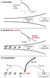 |
Fig. 1 Envisioned chronology of the formation of trans-Neptunian objects. I. Formation. An initial burst of planetesimal formation populates bodies in the primordial belt (PB) at ~20 au and the cold classicals at ~40–50 au). It is assumed that the shape of the cold classicals and the primordial belt size distributions are similar, both featuring a tapered exponential at high mass. II. Growth: Pebble accretion, acting preferentially on the massive bodies, alters the size distribution of the PB. Growth takes place in a gas-rich medium. This is the phase investigated in this work. III. Implantation. Neptune’s migration disperses the PB with a implantation fraction fimpl,P48 populating the dynamically hot bodies within 48 au (population P48). |
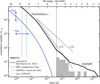 |
Fig. 2 Cumulative number distribution (N<m) of bodies in the cold belt and the dynamical hot P48. The cold belt is well described by the analytical fit of Kavelaars et al. (2021) (Equation (2)), whose shape is assumed to be identical to the distribution of the bodies in the primordial belt. Population P48 is reconstructed by taking all bodies brighter than Hr = 5 and within 48 au from the MPC database (histograms) while bodies 5 ≤ Hr ≤ 8.3 are assumed to follow the completeness-corrected distribution from OSSOS++. The corresponding cumulative mass function is given by the black curve. The conversion between mass and magnitude (top) assumes an albedo typical for hot belt bodies (see Appendix A). The dotted lines labeled p = −2.0 and p = −2.5 correspond to N<m ∝ m1+p with p = −2 indicating an equal amount of mass per logarithmically spaced mass bin (the corresponding indices in terms of a radius spectrum dN/dR ∝ Rq are q = −4 and q = −5.5, respectively). Pebble accretion operates to selectively grow the largest TNOs, flattening the size distribution. |
2 Model
This section consists of three parts. In Section 2.1, we reconstruct a population of TNOs that is complete, against which the model outcome can be evaluated. Section 2.2 describes the pebble accretion model, which is formulated in dimensionless units. While this approach makes the model more abstract, it avoids the need to introduce a specific disk model. Finally, in Section 2.3, we construct the MCMC likelihood function and outline the model parameters.
2.1 The mass function of the dynamical hot population
In Figure 2, we have reconstructed the present-day mass distribution of dynamically hot TNOs within 48 au, a population we refer to as P48. This distribution is composed of two parts. At high masses, we take the bodies directly from the Minor Planet Center (MPC) database3 and filter out the cold classicals by applying an ifree < 4° cut (Huang et al. 2022). Specifically, we assume that the data, which includes the entire hot belt, inner belt, 3:2 population (plutinos), 2:1 population (twotinos), as well as scattering TNOs, is complete for Hr < 5 bodies within a ≤ 48 au (Weryk et al. 2016; Petit et al. 2023).
We excluded 13 members that belong to the Haumea collisional family, as they are likely fragments ejected from Haumea during or after Neptune’s migration (Proudfoot & Ragozzine 2019), and are therefore unrelated to the prior pebble accretion process. To account for the lost mass of the Haumea impactor (which could be a moon of Haumea or a dwarf planet from the scattering disk depending on the hypothesis), we include a new body with a mass equal to 3% of Haumea’s (Vilenius et al. 2018; Pike et al. 2020) in our sample. Additionally, we add Neptune’s largest moon, Triton4, which is believed to be a captured moon from the primordial belt (Agnor & Hamilton 2006), as well as Pluto’s largest moon, Charon, which likely formed from a giant impact (Canup 2005). In total, 66 bodies constitute the high-mass portion of the P48 population (see Table A.1), reflecting our current best understanding of the dwarf planet size distribution.
Trans-Neptunian Objects dimmer than Hr = 5 in P48 are modeled on the debiased distribution of the hot belt5, based on the OSSOS++ survey (Petit et al. 2023). Their Figure 1 presents the differential distribution, which we fit by a broken power law
![Mathematical equation: $\[\Delta \frac{d \log _{10} N}{d H}= \begin{cases}0.95 H_r-3.45 & \left(5.0 \leq H_r \leq 6.8\right) \\ 0.55 H_r-0.73 & \left(6.8 \leq H_r \leq 8.3\right)\end{cases}\]$](/articles/aa/full_html/2025/03/aa53420-24/aa53420-24-eq1.png) (1)
(1)
where Δ = 0.25 dex is the bin spacing adopted by Petit et al. (2023). We further estimate that the hot classicals makes up 50% of the dynamical hot bodies in P48, based on population estimates of Hr < 8.7 objects: the hot belt contains 20 × 103 objects (Petit et al. 2023), while the inner belt, twotinos, plutinos, and scattering populations within a < 48 au contain 3, 4.4, 8, and 3 × 10³ objects, respectively (Petit et al. 2011; Volk et al. 2016; Chen et al. 2019). The fraction of hot belt TNOs in P48 is thus 20/(20 + 3 + 4.4 + 8 + 3) ≈ 0.5. Therefore, we multiply the number N that follows from Equation (1) by a factor 2 when reconstructing the P48 distribution (see Figure 3).
In Figure 2, the cumulative distribution of bodies in P48 is plotted alongside the debiased distribution of the cold belt, which is well described by an exponentially tapered power law (Kavelaars et al. 2021). Converted in terms of mass (see Appendix A), the mass function reads:
![Mathematical equation: $\[N_{>m}=N_{\text {pre }}\left(\frac{m}{m_{\mathrm{brk}}}\right)^{-\alpha} \exp \left[-\left(\frac{m}{m_{\mathrm{brk}}}\right)^\gamma\right],\]$](/articles/aa/full_html/2025/03/aa53420-24/aa53420-24-eq2.png) (2)
(2)
where for the cold belt α = 0.67, γ = 0.42, and the mass scale indicating the transition to the exponential cut-off regime, mbrk = 2 × 10²⁰ g (D ≈ 70 km). In Equation (2), Npre is a normalization factor, which, for the specified values of α and γ, can be expressed in terms of the total mass in the belt, mbelt, as Npre = mbelt/2.81mbrk. It is important to note that converting between magnitude Hr and mass depends on albedo, which varies between bodies in the hot and cold belts. Consequently, any similarity in the magnitude distributions of the cold and hot belt populations (Petit et al. 2023) does not necessarily imply similarity in the mass distributions. To account for this, we treat mbrk as a model parameter. Along with the total initial mass mimf of the primordial belt, this parameter defines the initial distribution prior to pebble accretion.
 |
Fig. 3 Implantation fractions for bodies of the primordial belt into the trojans, hot classicals, and P48. Numbers in bold are used in this work (see text for motivation) and others are given as context. The numbers for the Jupiter trojans follow Nesvorný et al. (2013) and those for the entire dynamically hot TNO population Nesvorný et al. (2016) and Huang (2023). |
2.2 Growth of bodies by pebble accretion
Not accounting for gravitational effects, a spherical body of radius R and mass m will sweep up pebbles at a rate dm/dt = πR2 ρpebΔv, where ρpeb is the mass density of pebbles and Δv the approach velocity. Defining q = m/m⋆ and σ = Δv/vK as the dimensionless mass and relative velocity with vK = rΩK as the Keplerian velocity corresponding to orbital radius of r, we can rewrite the accretion rate as
![Mathematical equation: $\[\frac{d q}{d t}=A_{\mathrm{geo}} \frac{\chi_{\bullet}^2 \sigma q^{2 / 3}}{t_0},\]$](/articles/aa/full_html/2025/03/aa53420-24/aa53420-24-eq3.png) (3)
(3)
where χ• is the physical-to-Hill radius ratio
![Mathematical equation: $\[\chi_{\bullet}=\frac{R}{r}\left(\frac{3 m_{\star}}{m}\right)^{1 / 3}=\left(\frac{9 m_{\star}}{4 \pi \rho_{\bullet} r^3}\right)^{1 / 3} \approx 10^{-4}-10^{-3},\]$](/articles/aa/full_html/2025/03/aa53420-24/aa53420-24-eq4.png) (4)
(4)
where ρ• the internal density of the planetary body and Ageo = π/32/3 ≈ 1.5. In addition, the characteristic growth timescale is
![Mathematical equation: $\[t_0=\frac{M_{\odot}}{\rho_{\mathrm{peb}} r^3 \Omega}\]$](/articles/aa/full_html/2025/03/aa53420-24/aa53420-24-eq5.png) (5)
(5)
![Mathematical equation: $\[=3.5 \times 10^4 \mathrm{yr}\left(\frac{Z_{\mathrm{peb}}}{0.01}\right)^{-1}\left(\frac{\Sigma_{\mathrm{gas}} r^2 / M_{\odot}}{0.01}\right)^{-1} \frac{H_{\mathrm{gas}} / r}{0.07} \frac{\Omega^{-1}}{20 ~\mathrm{yr}},\]$](/articles/aa/full_html/2025/03/aa53420-24/aa53420-24-eq6.png) (6)
(6)
where ![Mathematical equation: $\[\rho_{\mathrm{peb}}=Z_{\mathrm{peb}} \rho_{\mathrm{gas}}=Z_{\mathrm{peb}} \Sigma_{\mathrm{gas}} / \sqrt{2 \pi} H_{\mathrm{gas}}\]$](/articles/aa/full_html/2025/03/aa53420-24/aa53420-24-eq7.png) the mass density of pebbles in the midplane, Zpeb the corresponding local metallicity, Σgas the surface density of the gas and Hgas the gas pressure scale height. The disk aspect ratio h = Hgas/r can also be written
the mass density of pebbles in the midplane, Zpeb the corresponding local metallicity, Σgas the surface density of the gas and Hgas the gas pressure scale height. The disk aspect ratio h = Hgas/r can also be written
![Mathematical equation: $\[h=\sqrt{\frac{k_B T r}{\mu m_{\mathrm{u}} G m_{\odot}}}=0.069\left(\frac{T}{60 \mathrm{~K}}\right)^{1 / 2}\left(\frac{r}{20 ~\mathrm{au}}\right)^{1 / 2},\]$](/articles/aa/full_html/2025/03/aa53420-24/aa53420-24-eq8.png) (7)
(7)
where T is the temperature in the midplane and μ = 2.34mu the mean molecular weight of the gas.
The degree of coupling between particles and gas is quantified by the particle stopping time tstop, which represents the time for a particle to adjust its motion to that of gas. Its dimensionless equivalent, τs = ΩKtstop, is referred to as the aerodynamic size (in the literature, the Stokes number or St, is also common). In this work we define pebbles as particles of τs < 1. For the Epstein drag, τs can be expressed as τs = π(ρ•R)peb/2Σgas, indicating that the aerodynamic size is proportional to Rpeb.
The relative velocity Δv = σvK can be identified in one of three ways:
the eccentricity of planetesimals, Δv ≃ evK (σ = e), which is not considered in this work;
-
the headwind velocity of the gas. Due to the radial pressure gradient, the azimuthal motion of the gas lags the Keplerian motion by an amount Δv = ηvK (σ = η), where
![Mathematical equation: $\[\eta \equiv-\frac{1}{2} \frac{\partial \log P}{\partial \log r} h^2=4.9 \times 10^{-3}\left(\frac{\partial_{\log r} \log P}{-2}\right)\left(\frac{h}{0.07}\right)^2\]$](/articles/aa/full_html/2025/03/aa53420-24/aa53420-24-eq9.png) (8)
(8)(e.g., Weidenschilling 1977) is a parameterization of the radial pressure gradient. Pebbles with τs < 1 follow the gas, while planetesimals (τs ≫ 1) move at the Keplerian velocity. Hence, the pebble-planetesimal velocity is also ηvK;
the turbulent velocity Δv ≃ ℳcs (σ = ℳh), where ℳ is the Mach number of the turbulent flow and h is the disk aspect ratio.
Roughly, the highest of these velocities (e, η, or ℳh) determines Δv.
Gravitational focusing increases the accretion rate by a factor of (vesc/Δv)2 = 2Gm/R(Δv)2, where vesc is the escape velocity from its surface. In dimensionless units, the rate becomes
![Mathematical equation: $\[\frac{d q}{d t}=A_{\mathrm{Saf}} \frac{\chi q^{4 / 3}}{\left(\sigma+q^{1 / 3}\right) T},\]$](/articles/aa/full_html/2025/03/aa53420-24/aa53420-24-eq10.png) (9)
(9)
with ASaf = 2π/31/3 ≈ 4.4. Here, we add a term q1/3 in the denominator in order to account for the Keplerian shear component of the relative velocity, which becomes important when σ is low.
Gravitational focusing significantly enhances the growth rates of planetesimals. On the other hand, its efficacy is hampered by the more copious noncollisional scatterings of planetesimals – a process known as viscous stirring (Ida & Makino 1993) – or turbulent stirring (Ida et al. 2008), which increases Δv. For small pebbles tightly coupled to the gas, this is not a concern, because gas drag circularizes their orbits before the next encounter. Therefore, in contrast to planetesimals, there is no need to follow the evolution of Δv with time.
More potently, pebbles accrete by the settling mechanism, which is better known as pebble accretion (Ormel & Klahr 2010; Lambrechts & Johansen 2012). In pebble accretion, pebbles can be captured at distances much larger than R, after which the pebbles settle down in the gravitational potential. We adopt the numerically calibrated expression by Ormel & Liu (2018)6:
![Mathematical equation: $\[\frac{d q}{d t}=A_{\mathrm{peb}} \frac{q \tau_s}{t_0} f_{\mathrm{set}}^2 .\]$](/articles/aa/full_html/2025/03/aa53420-24/aa53420-24-eq11.png) (10)
(10)
Here Apeb = 12.3 and fset ≤ 1 is a modulation factor that suppresses accretion rates at low masses. It is a defining characteristic of pebble accretion that rates do not depend on the physical radius (or the nondimensional χ• parameter; Ormel 2017). In addition, we assumed the 3D accretion regime for pebbles in Equation (10), for which σ does not enter explicitly. The velocity matters in the modulation factor fset, however:
![Mathematical equation: $\[f_{\mathrm{set}}^2=\exp \left[-\left(\frac{\Delta v}{v_*}\right)^2\right] \quad \text { or } \quad f_{\mathrm{set}}^2=\left[1+a_{\mathrm{turb}}\left(\frac{\Delta v}{v_*}\right)^2\right]^{-3}.\]$](/articles/aa/full_html/2025/03/aa53420-24/aa53420-24-eq12.png) (11)
(11)
Here v* = (qp/τs)1/3vK and aturb = 0.33 (Liu & Ormel 2018). The first expression in Equation (11) holds for a laminar-dominated velocity field and the second for a turbulent-dominated Δv. In the case of a turbulent flow, Δv should be regarded as the rms value of an underlying velocity distribution that is isotropic (Ormel & Liu 2018).
Figure 4 presents the Safronov and settling growth rates as functions of mass. Here, the rates are expressed in terms of the growth timescale, tgr = m/(dm/dt), which is given in units of t0 (see Equation (5)). At low masses, accretion is dominated by gravitational focusing (Safronov limit; yellow curve). It is well known that in this limit, the growth timescale decreases with the mass: the runaway growth regime (Wetherill & Stewart 1989). Pebble accretion (the settling mechanism) is unimportant at low masses. However, at a mass scale that is a fraction of q* = σ3τs (the mass corresponding to σ ~ v*), the settling mechanism starts to become efficient, increasing the growth rate significantly (Visser & Ormel 2016). In the case of a turbulence-dominant velocity field, this transition is slightly less abrupt (thin line). Hence, bodies more massive than ~0.1 m* will undergo rapid growth, while those with m ≪ m* grow more slowly. Pebble accretion therefore has the potential to flatten the high-mass tail of the size distribution, illustrated in Figure 4 by the gray arrows.
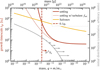 |
Fig. 4 Growth timescales for pebble accretion (settling mechanism, red) and Safronov accretion (gravitational focusing in the absence of gas drag; yellow) for a velocity parameter of σ = Δv/vK = 10−3, dimensionless stopping time τs = 2 × 10⁻³, and internal density parameter χ• = 5 × 10⁻⁴. The critical mass q* = σ3 τs (or rather a fraction of this number; vertical dashed line) indicates the point where the settling mechanism becomes operational. In the case where the approach velocity is due to turbulence, such that Δv follows a distribution, the transition is more gradual (thin red line). Pebble accretion acts on the high-mass tail of the distribution where the length of the arrows is proportional to the growth rate (Equation (10); gray). |
2.3 Model parameters and likelihood
An overview of the parameters used in the model is given in Table 1. The initial distribution of bodies is specified by the parameter mbrk and the initial mass of the belt mimf (see Equation (2)), which are uniformly sampled in the log space. The pebble properties are given by their dimensionless velocity σ, the dimensionless stopping time τs, and the total accreted pebbles mass mPeb. In addition to the continuous sampling of these parameters, the model also employs a binary switch for the nature of the velocity field, either laminar or turbulent. If the velocity is laminar, σ is identified with the normalized pressure gradient parameter η; if the velocity is turbulent, σ is identified with the Mach number of the turbulent velocity field. The velocity field matters in calculating the fset modulation factors (see Equation (11)).
In total, the sampling provides us with several hundred bodies, which covers the entire mass distribution. The mass of each of the bodies is integrated over time. We work in dimensionless units where time is normalized by t0 (Equation (5)) and mass by the mass of the Sun. The pebble accretion rate dq/dt is computed for each of these bodies, according to the collision rates given in Section 2.2. The bodies do not interact among themselves, and because dq/dt is an increasing function of q, the initial order of their masses stays preserved. Under these conditions, the calculation boils down to a set of ordinary differential equations, which we solve with the scipy.integrate.odeint library. Simultaneously with the increase in q, we decrease the mass of the pebble reservoir qpeb, whose initial value is also a parameter. When qpeb reaches 0, we stop the simulation and record the elapsed time t (in units of t0). This distribution is then weighted by the implantation factor fimpl, the ratio of the number of bodies in the present-day P48 to that in the primordial belt, to obtain the simulated distribution of bodies in P48.
The likelihood function is calculated by comparing the simulated distribution with the reconstructed distribution in the OSSOS++ domain and the observed number of bodies in the MPC domain (see Figure 2). To this end, the particles are binned by mass, with 10 bins covering the OSSOS++ region and 15 covering the MPC region; the bin width is about 0.2 dex. The number of bodies in the synthetic and observed distributions are then compared for each bin. In the OSSOS++ region, Gaussian statistics are assumed; in other words, the contribution to the log-likelihood of bin k equals
![Mathematical equation: $\[\ln P_k^{\mathrm{OSSOS}++}=-\frac{1}{2}\left(\frac{N_k-N_{\mathrm{sim}, k}}{\sigma_k}\right)^2-\frac{1}{2} \ln \left(2 \pi \sigma_k^2\right)\]$](/articles/aa/full_html/2025/03/aa53420-24/aa53420-24-eq13.png) (12)
(12)
where Nsim,k is the simulated number of bodies, Nk is the observed number of bodies in P48, as obtained from Equation (1), and σk represents the spread. The spread σk is also obtained from the debiased OSSOS++ distribution7. For the MPC part, we use binomial statistics to obtain the likelihood contribution:
![Mathematical equation: $\[\ln P_k^{\mathrm{MPC}}=\ln \mathcal{B}\left(N_k, N_{\text {sim}, k}, f_{\mathrm{impl}}\right) .\]$](/articles/aa/full_html/2025/03/aa53420-24/aa53420-24-eq14.png) (13)
(13)
Here ℬ(x, n, p) is the probability of drawing x successes out of n independent samples where each draw has probability p.
In addition, we apply two priors to the likelihood function, related to the following observations. First, the number of Jupiter trojans constrains the total mass of the primordial belt mimf + mpeb. Since the Jovian trojans are also thought to be captured from the same disk, the mass of bodies present in the primordial belt can be estimated using a numerically simulated implantation rate and the observed mass of the trojans (see Figure 3 and Nesvorný et al. 2013). The total pre-instability mass of the primordial belt falls in the range of 14–28 m⊕. Consequently, we add a term 𝒫PB to the likelihood function corresponding to a situation where the parameter μ = ln(mimf + mPeb) is normally distributed, centered around ln 20 m⊕ and with spread σ = 0.34. Second, the preservation of the dynamically cold classicals limits the mass of individual bodies. If any planetary-mass bodies formed in the primordial outer disk and were scattered out by a migrating Neptune, the cold classical belt would likely be overheated or even destroyed by the gravitational sweeping of such a planet. Therefore, the masses of the individual bodies making up the primordial belt could not have been too large. Petit et al. (1999) simulated the effect of massive protoplanets on the stability of the cold belt, and found a threshold mass of ~1 m⊕. To incorporate this mass constraint, we add a term ln 𝒫CC = −(m1/m⊕)2 to the log-likelihood function, which suppresses models favoring the formation of bodies beyond 1 Earth mass. The total log-likelihood is then
![Mathematical equation: $\[\ln \mathcal{P}=\sum_k \ln \mathcal{P}_k^{\mathrm{MPC}}+\sum_k \ln \mathcal{P}_k^{\mathrm{MPC}}+\ln \mathcal{P}^{\mathrm{CC}}+\ln \mathcal{P}^{\mathrm{PB}}.\]$](/articles/aa/full_html/2025/03/aa53420-24/aa53420-24-eq15.png) (14)
(14)
We conduct an MCMC analysis using emcee (Foreman-Mackey et al. 2013), marginalizing over the input parameters listed in Table 1.
Model parameters.
3 Results
The posterior values of the model parameters from the MCMC fit are summarized in Table 2. Four model suites are considered, each characterized by binary choices for the velocity field – either laminar (lami-) or turbulent (turb-) – and the particle components – a single particle size (1p) or two pebble sizes (2p). Models with two particle sizes feature two additional parameters: the aerodynamic size (τ2) and the mass fraction of the second component (f2).
List of model runs and posterior values for the MCMC simulations.
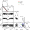 |
Fig. 5 MCMC posterior distribution of the single particle laminar model (lami-1p). The 16%, 50%, and 84% confidence levels are indicated above each histogram. The runs cluster around the line of constant τsσ3, which indicates a mass scale above which pebble accretion operates (panel b). High-velocity solutions, as in a smooth disk (σ = ηirr), have difficulty fitting the data (panel a). The mass of the accreted pebbles is lower than the mass of the initial popluation by around 0.4 dex (panel n). |
3.1 Simulations with a single particle component
Figure 5 presents the corner plot of the lami-1p model (laminar velocity field with one pebble size). The most striking feature is the correlation between the stopping time τs and the relative velocity (see panel b). The slope of this correlation is −3, which points to a mass scale where pebble accretion is initiated, q* = σ3τs. Specifically, we fit
![Mathematical equation: $\[C_{\tau \sigma} \equiv \log _{10} \tau_s \sigma^3=\log _{10} \tau_s+3 \log _{10}\left(\frac{\Delta v}{v_K}\right)=-10.05_{-0.12}^{+0.11}.\]$](/articles/aa/full_html/2025/03/aa53420-24/aa53420-24-eq44.png) (15)
(15)
In physical units, ![Mathematical equation: $\[m_*=10^{C_{\tau \sigma}} m_{\odot} \approx 1.6 \times 10^{23} \mathrm{~g}\]$](/articles/aa/full_html/2025/03/aa53420-24/aa53420-24-eq45.png) (or 10−5 m⊕; the actual mass where pebble accretion starts to dominate over Safronov accretion is ≈10% of this number; see Figure 4). For bodies of mass m > m*, pebble accretion is fully operational, whereas below m* pebble accretion is suppressed. Therefore, for m ≪ m*, the mass distribution tends to follow the IMF, as given by the mbrk and mimf parameters. However, due to the exponential tapering at high mass, the IMF cannot fit the high-mass end of the P48 bodies. Here pebble accretion acts to flatten the mass distribution (see Figure 4). Table 2 shows that about 5–8 Earth masses in pebbles are needed, an amount that is similar to the mass in the IMF.
(or 10−5 m⊕; the actual mass where pebble accretion starts to dominate over Safronov accretion is ≈10% of this number; see Figure 4). For bodies of mass m > m*, pebble accretion is fully operational, whereas below m* pebble accretion is suppressed. Therefore, for m ≪ m*, the mass distribution tends to follow the IMF, as given by the mbrk and mimf parameters. However, due to the exponential tapering at high mass, the IMF cannot fit the high-mass end of the P48 bodies. Here pebble accretion acts to flatten the mass distribution (see Figure 4). Table 2 shows that about 5–8 Earth masses in pebbles are needed, an amount that is similar to the mass in the IMF.
At high velocity the correlation starts to break down. Here, the combination of high σ and small τs renders pebble accretion very slow (Equation (10)) and allows ballistic encounters (Safronov focusing) to rival pebble accretion. As a result, the mass distribution at low mass is altered, which is demonstrated by the lami-1p-etairr model, which features a value of σ consistent with that of an irradiated disk. Figure 7 illustrates that in this model low-mass bodies accrete a significant amount of pebbles. As σ increases, this trend becomes more pronounced and results in poorer fits because the OSSOS++ part of the distribution can no longer be matched. This finding is unsurprising as the shape of the IMF was adopted from the cold classicals, which was already shown to fit the shape of hot classicals across the OSSOS++ range (Kavelaars et al. 2021; Petit et al. 2023). However, it also shows that accretion processes cannot maintain the shape of the low-mass part, at least not in conjunction also matching the high-mass tail. It lends further support to the primordial nature of the low-mass part of the TNO size distribution.
An additional concern for these small τs runs is that they take a long time (t/t0 is high). We can estimate the characteristic accretion time for pebble accretion from the pebble accretion rate (Equation (10)): ![Mathematical equation: $\[t \sim q / \dot{q} \sim t_0 / \tau_s\]$](/articles/aa/full_html/2025/03/aa53420-24/aa53420-24-eq46.png) , for fset ~ 1 (i.e., m > m*). This estimate agrees with Table 3 where we compiled t/t0 for selected model runs. We recall that the simulations are conducted in dimensionless parameter space, where we can hide our ignorance of, the pebble density, for example, which sets the value of t0 (Equation (5)). However, the pebble accretion mechanism requires gas-rich conditions and it must terminate before the lifetime of the gas-rich disk, typically estimated at ~5 Myr (Weiss et al. 2021). Therefore, a high t/t0 renders these models implausible. We return to the timescale constraints in Section 4.
, for fset ~ 1 (i.e., m > m*). This estimate agrees with Table 3 where we compiled t/t0 for selected model runs. We recall that the simulations are conducted in dimensionless parameter space, where we can hide our ignorance of, the pebble density, for example, which sets the value of t0 (Equation (5)). However, the pebble accretion mechanism requires gas-rich conditions and it must terminate before the lifetime of the gas-rich disk, typically estimated at ~5 Myr (Weiss et al. 2021). Therefore, a high t/t0 renders these models implausible. We return to the timescale constraints in Section 4.
Table 2 shows that a turbulent velocity field marginally improves the log-likelihood of the best model by an amount of +0.5. This specific run is characterized by a very low τs value (turb-1p-best entry in Table 3), which is disfavored in light of the above discussion. A higher τs run, following the τs−σ correlation (turb-1p-hitau) fits the data equally well. Figure 6a presents the cumulative distribution of several individual runs. All models overshoot the infliction point at m = 10−4 m⊕ and also tend to undershoot the final bin where the observed CMF terminates (with Triton) at m = 3 × 10⁻³ m⊕. These apparent mismatches are a consequence of the low number of TNOs at these masses, which can be understood from inspecting the differential distribution (on which the likelihood calculations are based). Figure 6b presents these fits for the MPC part of the distribution. Here, the error bars denote Poisson counting uncertainties. The bin to the right of m = 10−4 m⊕ with 0 bodies in the MPC is typically fitted with ≈2 bodies in the simulation, but this still has a Poisson likelihood of 13.5%. Similarly, the simulation runs are quite insensitive to the presence of the two most massive bodies (Pluto and Triton); statistically, the low number of high-m bodies do not carry much weight. As a result the runs that undershoot the cumulative curve in Figure 6a (e.g., turb-1p-best) statistically cannot be distinguished from those runs that include a larger τs (e.g., turb-1p-hitau) and those runs that contain more pebbles (e.g., turp-1p-himass).
3.2 A second particle component
The addition of a secondary component does not significantly improve the results. From Table 2, the Bayes factor (the difference in ln 𝒫) is 0.54 between the laminar models and 0.18 between the turbulence models. These values indicate that the added parameters have insignificant effects on the fits (Jeffreys 1998). This insensitivity is reflected in Table 2 by the proximity of the size of the secondary component (τ2) to that of the main component (τs) in the lami-2p and turb-2p models. Figure 6 presents this result graphically. The lami-2p-best run – the run where 𝒫 is the highest – hardly stands out from the other runs. Curiously, these models tend to be fitted by low τs (and τ2) and correspondingly high t0, indicating that these runs improve the fit for the OSSOS++ part of the distribution, rather than the high-mass MPC part. In other words, the low number of high-mass bodies in P48 prevents any meaningful fit for the high-mass end of the distribution, which makes the model insensitive to a second particle component.
While we do not find evidence for a binary distribution of pebbles, two points should be noted. First, the size distribution could still be a power law, which would ameliorate the fset transition in a similar way to that of the turbulence velocity field (Lyra et al. 2023). Second, the lack of evidence for a second component does not preclude its presence. A bigger sample of high-mass bodies is necessary to establish or discount its existence.
4 Implications
The MCMC calculations in the previous section demonstrate that both turbulent and laminar models fit the data. Here, we identify the laminar model with formation in a standard smooth disk, characterized by a spatially constant radial pressure parameter η (Equation (8)). Conversely, the turbulent model corresponds to formation within an environment where pebbles collect around a radial pressure maximum (η ≈ 0) such that velocities are dominated by turbulent motions. This can be identified with pebble rings seen in ALMA.
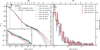 |
Fig. 6 Cumulative distributions (a) and histograms (b) of sample model runs. An implantation factor of fimpl = 2 × 10⁻³ has been applied, after which the simulated distributions can be compared to the P48 population (black). In (b) the low number of bodies (and large Poisson error bars) illustrate why the fits tend to be rather insensitive to the specifics at the high-mass end of the distribution. Runs featuring small τs are associated with high σ due to the degeneracy between these quantities (see Table 3). Runs with small τs are disfavored, however, as pebble accretion operates too slowly. |
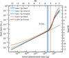 |
Fig. 7 Final vs initial mass for several simulation runs (see Table 3). The vertical lines denote 10% of m* = σ3 τsm⊙, which is the scale where pebble accretion begins. The dashed line is the identity line (y = x). Bodies ≳1022 grow their mass by several tenfold by pebble accretion and become dwarf planets. The gain in mass at low mass in the lami-1p-etairr and turb-1p-best is due to the slow pace of pebble accretion, allowing Safronov interactions to become important at low planetesimal masses. |
4.1 Formation in a pebble ring
Pebble rings are ubiquitous in ALMA imagery (Andrews et al. 2018; Bae et al. 2023). The containment of particles by pressure maxima is the leading explanation for the observed particles accumulation of particles in these rings. Around the pressure maximum location η ≈ 0 and the relative motion between pebbles and bigger bodies is due to turbulence. Studies have used the extent of rings in both the vertical and radial dimensions to constrain the diffusivity (the “turbulent alpha” of the gas). Specifically, this constrains the ratio of gas diffusivity over Stokes number of the particles, αD/τs. Rosotti (2023) compiled results from a number of works that measure the radial width of continuum rings (their Table 2), and found that the inferred αD/τs ranged from a low of 0.04 to values exceeding unity (the latter essentially implies that particles follow the pressure distribution). However, αD/τs obtained from the vertical extent of the dust layer are often inferred to be smaller, e.g., αD/τs ≈ 10−2 (Villenave et al. 2022). For simplicity, we adopt in the following a range in αD/τs between 0.01 and 0.4, which covers most of these measurements.
When we convert the diffusivity parameter αD to a root mean square (rms) particle velocity, we obtain8
![Mathematical equation: $\[\frac{\sigma^2}{\tau_s}=\frac{3 h^2}{2}\left(\frac{\alpha_D}{\tau_s}\right)_{\mathrm{ALMA}} \approx 7 \times 10^{-4}\left(\frac{h}{0.07}\right)^2\left(\frac{\alpha_D / \tau_s}{0.1}\right)_{\mathrm{ALMA}}\]$](/articles/aa/full_html/2025/03/aa53420-24/aa53420-24-eq47.png) (16)
(16)
where (αD/τs)ALMA is inferred from the extent of the ring in ALMA imagery, and h = 0.07 is our adopted value for the aspect ratio of the gas at the location of the primordial belt.
A further constraint to particle sizes in rings comes from the fragmentation barrier (Güttler et al. 2010; Birnstiel et al. 2011). When the gas is turbulent, the pebble-pebble relative velocity increases with the size (Stokes number) as ![Mathematical equation: $\[\Delta v_{\mathrm{pp}} \approx \mathcal{M} c_s \sqrt{2 \tau_s}\]$](/articles/aa/full_html/2025/03/aa53420-24/aa53420-24-eq48.png) (Ormel & Cuzzi 2007)9, where ℳ is the Mach number of the turbulent flow. The aerodynamic size is then determined by the condition Δvpp = vfrag, resulting in
(Ormel & Cuzzi 2007)9, where ℳ is the Mach number of the turbulent flow. The aerodynamic size is then determined by the condition Δvpp = vfrag, resulting in
![Mathematical equation: $\[\sigma \tau_s^{1 / 2}=\frac{\mathcal{M} c_s}{v_K} \tau_s^{1 / 2}=\frac{\Delta v_{\mathrm{pp}}}{2^{1 / 2} v_K} \lesssim 1.1 \times 10^{-4}\left(\frac{v_{\mathrm{frag}}}{1 \mathrm{~m} \mathrm{~s}^{-1}}\right) .\]$](/articles/aa/full_html/2025/03/aa53420-24/aa53420-24-eq49.png) (17)
(17)
These constraints are presented in Figure 8, together with the constraint on τsσ3 that we obtained from modeling the TNO size distribution (Table 2). The constraint on the extent of ALMA rings is almost orthogonal to the constraint from the TNO size distribution modeling (this study), allowing us to put meaningful constraints on τs and αD. Together, they point to an aerodynamic size in the range of τs ~ [3 × 10⁻³−4 × 10⁻²], a turbulent diffusivity of αD ~ [4 × 10⁻⁴−2 × 10⁻³], and a fragmentation threshold of vfrag ~ [1.7–3.2 m s−1].
These values are similar to what was found by Jiang et al. (2024) in a recent analysis, who assumed a fragmentation threshold of vfrag ~ 1 m s−1. Our results independently suggest that the particle fragmentation threshold amount is ~2 m s−1 in order for particles to grow to the inferred aerodynamic sizes. A higher fragmentation threshold is possible if the growth of particles is limited by, for example, bouncing (Zsom et al. 2010). A fragmentation velocity increase by a factor of 2 would increase the derived value of the fragmentation α in Jiang et al. (2024) by a factor of 4 to ~4 × 10⁻⁴, in line with our findings.
If the TNO population formed from a ring in which the pebbles are contained by pressure, it is natural to assume that the birth ring would have had a mass in pebbles similar to the accreted pebble mass mpeb ~ 10 m⊕. This allows us to constrain the characteristic timescale t0, Equation (5). Since ρpeb ~ mring/2πrWrHr, where Wr and Hr are the width and height of the ring, we obtain
![Mathematical equation: $\[t_0 \sim 4 \times 10^3 \mathrm{yr}\left(\frac{m_{\text {ring }}}{10 ~m_{\oplus}}\right)^{-1} \frac{W_r / r}{0.1} \frac{H_r / r}{0.01} \frac{\Omega^{-1}}{20 ~\mathrm{yr}}.\]$](/articles/aa/full_html/2025/03/aa53420-24/aa53420-24-eq50.png) (18)
(18)
If the pebble aerodynamic size is τs ~ 10−2, it would take a time ~t0/τs for these bodies to accrete the pebbles, i.e., ~0.4 Myr, for the geometrical factors Wr/r and Hr/r adopted above. This time falls within the typical lifetimes of the solar nebula disk (Weiss et al. 2021), implying that pebbles will be consumed before the disk dissipates. However, very wide rings (Wr/r ~ 1 or Hr/r ~ 0.1) would dilute the concentration of pebbles and render pebble accretion much slower.
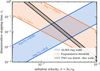 |
Fig. 8 Constraints on the particle aerodynamic size (Stokes number τs) and turbulence intensity of the gas, where σ is identified as the root mean square turbulent gas velocity. The constraints follow from simulating the TNO size distribution (run turb-1p, black line), ALMA ring morphological analysis (blue lines; Rosotti 2023), and particle fragmentation velocity (orange lines; the adopted value for the Keplerian velocity vK is the circular motion at 20 au). Under the assumption that the primordial belt featured conditions similar to ALMA rings, the degeneracy between τs and σ (or αD; Equation (16)) can be lifted and we find, τs ~ 0.01, αD ~ 10−3, and a fragmentation threshold of ~2 m s−1. |
4.2 A laminar disk
If pebbles are not entrained by a pressure maximum and freely drift inward, the relative velocity between planetesimals and pebbles is given by the global disk pressure gradient η. From Equation (8), σ = η ≈ 5 × 10⁻³ for a power-law index of pressure on radius of 2 and from the τs−σ relationship (Equation (15)), we then find an aerodynamic size of a mere τs = 7 × 10⁻⁴, which is rather small for pebbles. The radial drift timescale
![Mathematical equation: $\[t_{\mathrm{drift}}=\frac{r}{v_r}=\frac{1}{2 \eta \tau_s \Omega}\]$](/articles/aa/full_html/2025/03/aa53420-24/aa53420-24-eq51.png) (19)
(19)
![Mathematical equation: $\[=2 \times 10^6 ~\mathrm{yr}\left(\frac{\eta}{5 \times 10^{-3}}\right)^{-1}\left(\frac{\tau_s}{7 \times 10^{-4}}\right)^{-1}\left(\frac{r}{20 ~\mathrm{au}}\right)^{3 / 2}\]$](/articles/aa/full_html/2025/03/aa53420-24/aa53420-24-eq52.png) (20)
(20)
already rivals the disk lifetime, suggesting that particles hardly drift. In addition, the growth of planetesimals by such small particles would be excruciatingly slow, tgr ~ t0/τs ~ 50 Myr for the parameters listed in Equation (5), far exceeding the lifetime of the gas disk. A growth timescale ≲106 yr would therefore imply a (midplane) dust-to-gas ratio Zpeb ~ 1, which seems unlikely for small τs particles. In summary, it is unlikely that TNOs could accrete pebbles from an inward-drifting pebble stream in the standard, laminar disk model.
In addition, pebble accretion in a laminar disk is lossy (Ormel 2017; Lin et al. 2018). In the scenario where the birth ring is supported by pressure, all pebbles can (eventually) be accreted. That is, the efficiency is near 100%. This contrasts with the smooth disk scenario, where pebbles that fail to be accreted are lost. Consequently, the total mass in pebbles required for accretion, mneeded, exceeds the mass in pebbles actually accreted (mpeb). In a laminar disk, we can estimated mneeded as
![Mathematical equation: $\[\begin{aligned}m_{\text {needed }} & \sim 2 \pi r v_r \rho_{\mathrm{peb}} H_{\mathrm{peb}} t \sim 4 \pi M_{\odot} \eta h \tau_s \sqrt{\frac{\alpha_z}{\alpha_z+\tau_s}} \frac{t}{t_0} \\& \sim 1.4 \times 10^3 ~m_{\oplus}\left(\frac{h}{0.07}\right)^3\left(\frac{\alpha_z / \tau_s}{1}\right)^{1 / 2} \frac{t}{t_0 / \tau_s}\end{aligned}\]$](/articles/aa/full_html/2025/03/aa53420-24/aa53420-24-eq53.png) (21)
(21)
where t is the duration of the pebble accretion, ![Mathematical equation: $\[H_{\mathrm{peb}}=h r \sqrt{\alpha_z /\left(\alpha_z+\tau_s\right)}\]$](/articles/aa/full_html/2025/03/aa53420-24/aa53420-24-eq54.png) the pebble scale height (Dubrulle et al. 1995), and ρpeb the pebble density for which we substituted Equation (5). In the second line, we used again t ~ t0/τ. Equation (21) highlights that a great number of pebbles – far exceeding the mass actually accreted (mpeb) – is required, underscoring the inefficiency of pebble accretion in the primordial belt in a laminar setting. For small τs, the problem is that pebbles are not sufficiently concentrated in the midplane, whereas large τs implies a short duration of pebbles in the primordial belt.
the pebble scale height (Dubrulle et al. 1995), and ρpeb the pebble density for which we substituted Equation (5). In the second line, we used again t ~ t0/τ. Equation (21) highlights that a great number of pebbles – far exceeding the mass actually accreted (mpeb) – is required, underscoring the inefficiency of pebble accretion in the primordial belt in a laminar setting. For small τs, the problem is that pebbles are not sufficiently concentrated in the midplane, whereas large τs implies a short duration of pebbles in the primordial belt.
All these concerns would be reduced considerably when the disk is colder. Expressed in terms of the disk aspect ratio (h ∝ T1/2), η ∝ h2 and therefore τs ∝ σ−3 ∝ h−6 from Equation (15). For example, when h = 0.05 (about 35 K at 20 au; see Equation (7)), τs ≈ 6 × 10⁻³, a factor of 10 increase, the drift timescale reduces by a factor of 4 compared to Equation (19), the growth timescale may fall below the lifetime of the disk, and the required pebble mass, mneeded, to values below 500 m⊕. These numbers are within the realm of pebble accretion models (Lambrechts et al. 2019), although on the high side. A question that arises, however, is where these 500 m⊕ in solids would end up as the Solar System’s giant planets, while enriched, are not dominated in metals.
5 Discussion
5.1 Pebble accretion in the cold classical belt?
The absence of Hr < 5 bodies in the cold classical belt strongly suggests that pebble accretion did not play a significant role in the formation of these objects. Compared to the primordial belt, which has an estimated mass of ~20 m⊕, the cold belt is four orders of magnitude less massive (Kavelaars et al. 2020). If accretion is local, as in the turbulent model, the far smaller number of bodies in the cold belt implies a significantly reduced pebble density (ρpeb), which would make growth by pebble accretion ineffective. Alternatively, in the laminar scenario the number of pebbles that could have drifted through would be much greater. However, the drawbacks outlined in the previous section would only intensify. The greater distance of the cold belt (~40 au instead of ~20 au) and the correspondingly higher aspect ratio h, would increase the characteristic growth timescale t0/τs, the pebble drift timescale tdrift (Equation (19)) and the total mass of the pebble reservoir (mneeded; Equation (21)) to levels that become unrealistic. In addition, the conditions in the cold belt may have been such to inherently prevent pebble accretion from being triggered, i.e., m ≪ m*. The brightest cold classical is the binary (79360) Sila-Nunam (Huang et al. 2022) with an estimated system mass of 1.1 × 10²² g (Grundy et al. 2012) (D ≈ 280 km). From Figure 7, it is evident that these bodies barely fulfill the criterion for pebble accretion. While the specific conditions in the cold classical belt may differ, the parameters involved in setting the value of m* do not help. First, the higher η would increase m* and, second, a lower τs, while it would bring down m*, would slow down pebble accretion to levels that make it unviable. In conclusion, it is highly improbable that the bodies in the cold belt grew substantially from a passing swarm of pebbles.
5.2 Formation time constraints
Recently, Cañas et al. (2024) also investigated the growth of TNOs by pebble accretion. Their approach is complementary to ours. In particular, their study emphasizes the composition and internal density of TNOs. A key constraint is that small TNOs of radius 50–100 km could not have formed too quickly as radiogenic heating (primarily Al-26 decay at a half-life of 0.7 Myr; Norris et al. 1983) would have melted these bodies and reduced their porosity. This outcome is in contrast with observationally inferred densities of TNOS, implying that these TNOs have retained significant porosity (Bierson & Nimmo 2019).
Cañas et al. (2024) addressed this conundrum by hypothesizing that the initial distribution of TNOs formed through streaming instabilities dominated by large, ice-rich pebbles. Processes such as photodesorption could have resulted in a compositional dichotomy where ice is effectively transferred to the larger particles that settled to the midplane layers that were shielded from stellar UV irradiation. Cañas et al. (2024) argue that streaming instability would favor the larger ice-rich pebbles over the smaller Al-26 rich ones. Hence, the first-generation planetesimals were low in Al-26 and the early heating problem outlined by Bierson & Nimmo (2019) is avoided. Subsequently, these bodies accreted smaller, more water-poor, and denser pebbles over much longer timescales when heating by Al-26 decay is less significant.
Alternatively, TNOs may have formed late, only after several half-lives of Al-26 (Bierson & Nimmo 2019). This scenario implies that the conditions necessary for the primordial belt to form only emerged after several million years. Subsequently, pebble accretion could proceed without significant heating constraints. However, it would then be limited by the remaining time of the gaseous disk. Formation in a ring setting, where accretion timescales are short (~1 Myr) is then the preferred scenario.
5.3 TNOs formation by planetesimal accretion
An alternative to formation of TNOs by pebbles is growth among the planetesimal population itself (e.g., Kenyon & Bromley 2004). In this scenario accretion first proceeds through a rapid runaway growth phase (Wetherill & Stewart 1989), followed by a slower oligarchic growth phase (Kokubo & Ida 1998). Runaway growth conditions require that the initial population of bodies of mass m0 is dynamically quiescent (zero eccentricity), such that gravitational focusing becomes more effective for higher mass bodies. During runaway growth, a small number of bodies of mass much higher than m0 emerge on a timescale that is a fraction of the collision timescale among the initial population, tcoll,0. The distribution evolves into a mass spectrum dN/dm ∝ m−2.5 (Kokubo & Ida 1996; Barnes et al. 2009; Ormel et al. 2010b; Morishima et al. 2013). During the subsequent oligarchic growth, the most massive bodies separate from the continuous mass distribution, resulting in a flattening of the cumulative mass function. However, these oligarchs dynamically excite the planetesimal population, increasing their eccentricities and significantly slowing down growth.
The similarity of the TNO mass distribution to a p = −2.5 power law (see Figure 2) has been interpreted as evidence for a runaway growth origin (Ormel et al. 2010a; Kenyon & Bromley 2012; Morishima 2017). For the tapered-exponential distribution of Equation (2), it is natural to let m0 coincide with the mass scale where most of the population mass resides (i.e., m0 ~ 4mbrk ≈ 1021 g; see Appendix A), corresponding to a radius of about 50 km. The initial collision timescale then evaluates
![Mathematical equation: $\[\begin{aligned}t_{\mathrm{col}, 0} & \sim \frac{\rho_{\bullet} R}{\sum_{\mathrm{pltm} \Omega}}=\frac{2 \pi r W_r \rho_{\bullet} R}{\left(G m_{\odot} / r^3\right)^{1 / 2} m_{\mathrm{PB}}} \\& =67 ~\mathrm{Myr}\left(\frac{m_{\mathrm{PB}}}{20 ~m_{\oplus}}\right)^{-1}\left(\frac{r}{20 ~\mathrm{au}}\right)^{7 / 2} \frac{W_r / r}{0.2} \frac{\rho_{\bullet}}{1 \mathrm{~g~cm}^{-3}} \frac{R}{50 \mathrm{~km}},\end{aligned}\]$](/articles/aa/full_html/2025/03/aa53420-24/aa53420-24-eq55.png) (22)
(22)
where mPB is the mass of the primordial belt and Wr/r its fractional width. Unlike pebble accretion, planetesimal-driven growth does not need to be completed before the gas disk disperses, but it must conclude before the onset of the dynamical instability. The survival of the binary Jupiter trojan Patroclus–Menoetius puts constraints on the level of dynamical interactions in the precursor primordial belt. Specifically, Nesvorný et al. (2018) find a surviving probability exponentially decaying by a factor of 10 for every 100 Myr. Studies simulating the timing of the giant planet instability are consistent with these constraints (de Sousa et al. 2020). Thus, while these constraints limit the time for collisional processing in the primordial belt, the runaway growth phase is likely to have been sufficiently rapid (Equation (22)) to establish the p = −2.5 mass spectrum.
However, the TNO size distribution flattens at high mass, suggesting that the high-mass bodies (Triton, Pluto, Eris) accreted significantly more mass than their low-mass counter-parts. This characteristic is a hallmark of oligarchic growth, but it could also be achieved with pebble accretion (see, e.g., the lami-1p-himass model in Figure 6). Oligarchic growth, however, proceeds much more slowly than runaway growth and it may be challenging to meet the aforementioned timescale constraints. Alternatively, the runaway growth phase could have continued until Pluto-sized bodies formed, resulting in a continuous p = −2.5 mass spectrum, but with the subsequent stochastic implantation retaining a much higher fraction of TNO dwarf planets. In order to determine whether planetesimal or pebble accretion was the dominant formation mechanism, future simulations are needed to evaluate the scenarios under equivalent conditions. These efforts would greatly benefit from a more extensive and complete sample of TNOs.
5.4 The definition of a dwarf planet
The International Astronomical Union (IAU) defines a dwarf planet as “an object in orbit around the Sun that is large enough to pull itself into a nearly round shape but has not been able to clear its orbit of debris”10. While planetesimals that formed through SI can exhibit irregular shapes (as exemplified by Arrokoth’s bi-lobed structure), significant pebble accretion would naturally lead to more spherical bodies through the slow settling of material and the isotropy of the accretion process. Therefore, a body grown by pebble accretion with mfinal ≫ minit is expected to have a nearly round shape. Specifically, if we set the mass gain factor at 10, mfinal = 10minit, our simulations indicate that TNOs with masses greater than ~10−4m⊕ (or 6 × 10²³ g, comparable to Orcus) would fulfill the IAU requirement of dwarf planet (Figure 7). Future stellar occultations of TNOs are essential to test this hypothesis.
6 Conclusions
In this study, we investigated a scenario in which high-mass trans-Neptunian objects (TNOs) accreted pebbles before being implanted into their current locations. The characteristics of the TNO size distribution suggest that the dynamically hot bodies featured processing at the high-mass end, where the distribution significantly flattens (see Figure 2). This finding aligns with the pebble accretion mechanism, which operates preferentially on the most massive bodies, those exceeding the critical mass threshold m* (Figure 4). Focusing on a carefully selected sample of dynamically hot TNOs within 48 au, for which we argue the population is complete (Hr < 5 for bodies in the Minor Planet Survey and Hr < 8.3 for bodies in OSSOS++), we performed an MCMC analysis to best reproduce the observed present-day size distribution. This analysis allowed us to constrain the key parameters that describe the pebble accretion process, specifically the pebble aerodynamic size (τs) and the pebble-planetesimal velocity (Δv).
Our main conclusions are the following:
- 1
The TNO size distribution tightly constrains the combination of the TNO-pebble relative velocity Δv and pebble aerodynamic size τs in the primordial belt (Table 2 and Equation (15)). This corresponding threshold mass m*, implies that bodies above ~1022 g have enjoyed significant growth by pebble accretion (see Figure 7). While simulations featuring τs smaller than ~10−3 would formally fit the data, they imply very long accretion times, which rival the lifetime of the disk. Bodies exceeding m* increase their mass several tenfold and become dwarf planets (see Figure 7);
- 2
The data can be fitted with either a laminar or a turbulent velocity field. There is at present no evidence of a second pebble size. This stems mainly from the lack of bodies in the high-mass tail of the TNO distribution, which render the fit insensitive to this part;
- 3
TNOs likely did not form in a laminar disk. In such an environment, the radial pressure gradient would imply the particle aerodynamic size τs ≲ 10−3. Such small pebbles couple too well to the gas for pebble accretion to be effective. It would have made the process too slow in comparison to disk lifetimes. In addition, pebble accretion in smooth disks would put enormous demands on the total mass of pebbles that must have passed through the primordial belt (Equation (21), most of which do not get accreted). These issues would be mitigated, however, in a cold disk environment;
- 4
Most likely, pebble accretion proceeded locally, under conditions where pebbles are entrained by pressure and could not escape from the birth ring. In this case, η = 0 and the relative velocity is due to turbulence. These conditions would resemble the observed continuum millimeter emission from continuum rings by ALMA. The inferred (σ, τs) relation from this work can be combined with the constraints that the extent of the rings provide to give a preferred pebble aerodynamic size of τs ≈ 10−2. Pebble accretion could have been complete in ~0.1–1 Myr.
Future surveys like CLASSY (Fraser et al. 2022) and especially the advent of the Vera C. Rubin Observatory (Vera C. Rubin Observatory LSST Solar System Science Collaboration 2021) will greatly expand the TNO inventory by many times over. This will allow us to further constrain the pebble accretion process and deepen our understanding of planet formation in greater detail.
Acknowledgements
This work is supported by the National Natural Science Foundation of China under grant No. 12473065, 12233004, and 12250610189. Y.H. acknowledges funding support from Tsinghua University and National Observatory of Japan. The authors appreciate the referee for a thoughtful report, B. Gladman and E. Kokubo for useful discussions, and J.-M. Petit for providing the original OSSOS++ data.
Appendix A TNO masses
Kavelaars et al. (2021) modeled the magnitude distribution of the cold belt as
![Mathematical equation: $\[N\left(<H_r\right)=10^{\alpha^{\prime}\left(H_r-H_0\right)} \exp \left[-10^{-\beta\left(H_r-H_B\right)}\right] .\]$](/articles/aa/full_html/2025/03/aa53420-24/aa53420-24-eq56.png) (A.1)
(A.1)
where Hr is the OSSOS magnitude, α′ is the slope at low brightness objects, β describes the strength of the exponential tapering, which kicks in at Hr ~ HB, and H0 is a normalization parameter. If we define a mass-magnitude relation as
![Mathematical equation: $\[m=m_B 10^{-3 H_r / 5}\]$](/articles/aa/full_html/2025/03/aa53420-24/aa53420-24-eq57.png) (A.2)
(A.2)
we can relate the parameters appearing in Equation (A.1) to the cumulative distribution defined in Equation (2):
![Mathematical equation: $\[\gamma=\frac{5}{3} \beta ; \quad \alpha=\frac{5}{3} \alpha^{\prime} ; \quad \frac{m_B}{m_{\mathrm{brk}}}=10^{\beta H_B / \gamma} ; \quad N_{\mathrm{pre}}=10^{-\alpha^{\prime} H_0}\left(\frac{m_B}{m_{\mathrm{bkr}}}\right)^\alpha .\]$](/articles/aa/full_html/2025/03/aa53420-24/aa53420-24-eq58.png) (A.3)
(A.3)
With α′ = 0.4 and β = 0.252 (Kavelaars et al. 2021), we obtain α = 0.67 and γ = 0.42. We adopt the mass-magnitude conversion of Petit et al. (2023), where in Equation (A.2)
![Mathematical equation: $\[m_B=9.685 \times 10^{23} \mathrm{~g}\left(\frac{\rho_{\bullet} v^{-1.5}}{1 \mathrm{~g} \mathrm{~cm}^{-3}}\right)\]$](/articles/aa/full_html/2025/03/aa53420-24/aa53420-24-eq59.png) (A.4)
(A.4)
with v the albedo. For the cold belt, we take v = 0.15 and ρ• = 1 g cm−3 (Petit et al. 2023), which, with β = 0.252 and HB = 8.1 (Kavelaars et al. 2021), amounts to a breaking mass of mbkr = 2.3 × 10²⁰ g and a prefactor for the cold belt Ncold = Npre = 1.9 × 10⁴. For reference, the total mass, integrating Equation (2), amounts to
![Mathematical equation: $\[m_{\mathrm{tot}}=\frac{\Gamma[(1-\alpha) / \gamma]}{\gamma} m_{\mathrm{bkr}} N_{\mathrm{pre}}=2.81 m_{\mathrm{bkr}} N_{\mathrm{pre}},\]$](/articles/aa/full_html/2025/03/aa53420-24/aa53420-24-eq60.png) (A.5)
(A.5)
which equals 2.0 × 10⁻³ m⊕ for the cold belt. In addition, the characteristic mass of the population, defined as the ratio of the second to first moment of the mass distribution, is m* = 2 Γ[(2 − α)/γ]/Γ[(1 − α)/γ] = 3.97 mbkr.
For the hot belt, Petit et al. (2023) have shown that the shape of the magnitude distribution is the same as the cold belt with the number elevated by a factor of 2.2. This would nevertheless amount to a different shape for the mass distribution (Equation (2)) since the albedos of the hot and cold belts differ, as is commonly assumed. Specifically, we take ν = 0.08 and ρ• = 1 g cm−3 for bodies in P48. However, at high mass it is known that the mass-magnitude relationship represented by Equations (A.2) and (A.6) breaks (see Figure A.1). Several TNOs have mass estimates (those in P48 are listed in Table A.1) and we can use them to fit a mass-radius relationship for the high-mass end:
![Mathematical equation: $\[m=m_{\mathrm{tr}} 10^{-p_{\mathrm{hm}}\left(H_r-H_{\mathrm{tr}}\right)} \quad\left(m>m_{\mathrm{tr}}\right).\]$](/articles/aa/full_html/2025/03/aa53420-24/aa53420-24-eq61.png) (A.6)
(A.6)
Thus, at the point (Htr, mtr) the mass-magnitude relationship transitions from the low-mass expression (Equation (A.2)) to Equation (A.6), valid at high mass. Performing the fit, we obtain Htr = 4.12 and phm = 0.3638.
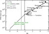 |
Fig. A.1 Mass-magnitude relationship for the hot main belt. At low mass we adopt the relationship given by Petit et al. (2023), Equations (A.2) and (A.6) (dashed line). At high mass we fit a power-law relationship to the TNOs for which the mass is known. |
All TNOs in the MPC sample.
References
- Abod, C. P., Simon, J. B., Li, R., et al. 2019, ApJ, 883, 192 [Google Scholar]
- Adams, E. R., Gulbis, A. A. S., Elliot, J. L., et al. 2014, AJ, 148, 55 [Google Scholar]
- Agnor, C. B., & Hamilton, D. P. 2006, Nature, 441, 192 [NASA ADS] [CrossRef] [Google Scholar]
- Andrews, S. M., Huang, J., Pérez, L. M., et al. 2018, ApJ, 869, L41 [NASA ADS] [CrossRef] [Google Scholar]
- Bae, J., Isella, A., Zhu, Z., et al. 2023, in Astronomical Society of the Pacific Conference Series, 534, eds. S. Inutsuka, Y. Aikawa, T. Muto, K. Tomida, & M. Tamura, 423 [Google Scholar]
- Bannister, M. T., Gladman, B. J., Kavelaars, J. J., et al. 2018, ApJS, 236, 18 [CrossRef] [Google Scholar]
- Barnes, R., Quinn, T. R., Lissauer, J. J., & Richardson, D. C. 2009, Icarus, 203, 626 [Google Scholar]
- Bernardinelli, P. H., Bernstein, G. M., Sako, M., et al. 2022, ApJS, 258, 41 [NASA ADS] [CrossRef] [Google Scholar]
- Bierson, C. J., & Nimmo, F. 2019, Icarus, 326, 10 [NASA ADS] [CrossRef] [Google Scholar]
- Birnstiel, T., Ormel, C. W., & Dullemond, C. P. 2011, A&A, 525, A11 [NASA ADS] [CrossRef] [EDP Sciences] [Google Scholar]
- Brown, M. E. 2008, The Largest Kuiper Belt Objects, eds. M. A. Barucci, H. Boehnhardt, D. P. Cruikshank, & A. Morbidelli, The Solar System Beyond Neptune (Tucson: University of Arizona Press) [Google Scholar]
- Brozović, M., & Jacobson, R. A. 2024, AJ, 167, 256 [Google Scholar]
- Cañas, M. H., Lyra, W., Carrera, D., et al. 2024, Planet. Sci. J., 5, 55 [CrossRef] [Google Scholar]
- Canup, R. M. 2005, Science, 307, 546 [NASA ADS] [CrossRef] [Google Scholar]
- Chen, Y.-T., Gladman, B., Volk, K., et al. 2019, AJ, 158, 214 [NASA ADS] [CrossRef] [Google Scholar]
- Cuzzi, J. N., Hogan, R. C., Paque, J. M., & Dobrovolskis, A. R. 2001, ApJ, 546, 496 [NASA ADS] [CrossRef] [Google Scholar]
- de Sousa, R. R., Morbidelli, A., Raymond, S. N., et al. 2020, Icarus, 339, 113605 [NASA ADS] [CrossRef] [Google Scholar]
- Doressoundiram, A., Peixinho, N., Bergh, C. d., et al. 2002, AJ, 124, 2279 [NASA ADS] [CrossRef] [Google Scholar]
- Drązkowska, J., Bitsch, B., Lambrechts, M., et al. 2023, in Astronomical Society of the Pacific Conference Series, 534, eds. S. Inutsuka, Y. Aikawa, T. Muto, K. Tomida, & M. Tamura, 717 [Google Scholar]
- Dubrulle, B., Morfill, G., & Sterzik, M. 1995, Icarus, 114, 237 [Google Scholar]
- Fernández-Valenzuela, E., Pinilla-Alonso, N., Stansberry, J., et al. 2021, Planet Sci. J., 2, 10 [Google Scholar]
- Foreman-Mackey, D., Hogg, D. W., Lang, D., & Goodman, J. 2013, PASP, 125, 306 [Google Scholar]
- Fraser, W. C., Brown, M. E., Morbidelli, A., Parker, A., & Batygin, K. 2014, ApJ, 782, 100 [Google Scholar]
- Fraser, W., Lawler, S., Ashton, E., et al. 2022, in AAS/Division for Planetary Sciences Meeting Abstracts, 54, 414.01 [Google Scholar]
- Gladman, B., Marsden, B. G., & Vanlaerhoven, C. 2008, The Solar System Beyond Neptune, 43, Nomenclature in the Outer Solar System, eds. M. A. Barucci, H. Boehnhardt, D. P. Cruikshank, & A. Morbidelli (Tucson University of Arizona Press) [Google Scholar]
- Gomes, R. S. 2003, Icarus, 161, 404 [Google Scholar]
- Grundy, W., Benecchi, S., Rabinowitz, D., et al. 2012, Icarus, 220, 74 [Google Scholar]
- Grundy, W. M., Noll, K. S., Roe, H. G., et al. 2019, Icarus, 334, 62 [CrossRef] [Google Scholar]
- Güttler, C., Blum, J., Zsom, A., Ormel, C. W., & Dullemond, C. P. 2010, A&A, 513, A56 [Google Scholar]
- Huang, Y. 2023, Dynamics of transneptunian objects under the influence of a rogue planet, PhD Thesis (Vancouver, Canada: University of British Columbia) [Google Scholar]
- Huang, Y., Gladman, B., & Volk, K. 2022, ApJS, 259, 54 [Google Scholar]
- Ida, S., & Makino, J. 1993, Icarus, 106, 210 [NASA ADS] [CrossRef] [Google Scholar]
- Ida, S., Guillot, T., & Morbidelli, A. 2008, ApJ, 686, 1292 [Google Scholar]
- Jeffreys, H. 1998, The Theory of Probability (Oxford University Press) [Google Scholar]
- Jiang, H., Macías, E., Guerra-Alvarado, O. M., & Carrasco-González, C. 2024, A&A, 682, A32 [NASA ADS] [CrossRef] [EDP Sciences] [Google Scholar]
- Jones, R., Gladman, B., Petit, J.-M., et al. 2006, Icarus, 185, 508 [Google Scholar]
- Kavelaars, J., Lawler, S. M., Bannister, M. T., & Shankman, C. 2020, The Trans-Neptunian Solar System, Perspectives on the distribution of orbits of distant Trans-Neptunian objects (Elsevier) [Google Scholar]
- Kavelaars, J. J., Petit, J.-M., Gladman, B., et al. 2021, ApJ, 920, L28 [NASA ADS] [CrossRef] [Google Scholar]
- Kenyon, S. J., & Bromley, B. C. 2004, AJ, 128, 1916 [Google Scholar]
- Kenyon, S. J., & Bromley, B. C. 2012, AJ, 143, 63 [NASA ADS] [CrossRef] [Google Scholar]
- Kokubo, E., & Ida, S. 1996, Icarus, 123, 180 [Google Scholar]
- Kokubo, E., & Ida, S. 1998, Icarus, 131, 171 [Google Scholar]
- Lacerda, P., & Jewitt, D. C. 2007, AJ, 133, 1393 [NASA ADS] [CrossRef] [Google Scholar]
- Lambrechts, M., & Johansen, A. 2012, A&A, 544, A32 [NASA ADS] [CrossRef] [EDP Sciences] [Google Scholar]
- Lambrechts, M., Morbidelli, A., Jacobson, S. A., et al. 2019, A&A, 627, A83 [NASA ADS] [CrossRef] [EDP Sciences] [Google Scholar]
- Levison, H. F., Morbidelli, A., VanLaerhoven, C., Gomes, R., & Tsiganis, K. 2008, Icarus, 196, 258 [NASA ADS] [CrossRef] [Google Scholar]
- Lin, J. W., Lee, E. J., & Chiang, E. 2018, MNRAS, 480, 4338 [Google Scholar]
- Liu, B., & Ji, J. 2020, Res. Astron. Astrophys., 20, 164 [Google Scholar]
- Liu, B., & Ormel, C. W. 2018, A&A, 615, A138 [NASA ADS] [CrossRef] [EDP Sciences] [Google Scholar]
- Lyra, W., Youdin, A. N., & Johansen, A. 2021, Icarus, 356, 113831 [CrossRef] [Google Scholar]
- Lyra, W., Johansen, A., Cañas, M. H., & Yang, C.-C. 2023, ApJ, 946, 60 [CrossRef] [Google Scholar]
- Malhotra, R. 1993, Nature, 365, 819 [CrossRef] [Google Scholar]
- McKinnon, W. B., Richardson, D. C., Marohnic, J. C., et al. 2020, Science, 367, aay6620 [NASA ADS] [CrossRef] [Google Scholar]
- Morbidelli, A., Levison, H. F., Tsiganis, K., & Gomes, R. 2005, Nature, 435, 462 [Google Scholar]
- Morgado, B. E., Sicardy, B., Braga-Ribas, F., et al. 2023, Nature, 614, 239 [NASA ADS] [CrossRef] [Google Scholar]
- Morishima, R. 2017, Icarus, 281, 459 [Google Scholar]
- Morishima, R., Golabek, G. J., & Samuel, H. 2013, Earth Planet. Sci. Lett., 366, 6 [Google Scholar]
- Müller, T., Lellouch, E., & Fornasier, S. 2020, The Trans-Neptunian Solar System, (Elsevier) 153 [Google Scholar]
- Napier, K. J., Lin, H. W., Gerdes, D. W., et al. 2024, Planet. Sci. J., 5, 50 [NASA ADS] [CrossRef] [Google Scholar]
- Nesvorný, D. 2015, AJ, 150, 73 [CrossRef] [Google Scholar]
- Nesvorný, D., Youdin, A. N., & Richardson, D. C. 2010, AJ, 140, 785 [Google Scholar]
- Nesvorný, D., Vokrouhlický, D., & Morbidelli, A. 2013, ApJ, 768, 45 [CrossRef] [Google Scholar]
- Nesvorný, D., Vokrouhlický, D., & Roig, F. 2016, ApJ, 827, L35 [CrossRef] [Google Scholar]
- Nesvorný, D., Vokrouhlický, D., Bottke, W. F., & Levison, H. F. 2018, Nat. Astron., 2, 878 [Google Scholar]
- Nesvorný, D., Li, R., Youdin, A. N., Simon, J. B., & Grundy, W. M. 2019, Nat. Astron., 3, 808 [CrossRef] [Google Scholar]
- Noll, K. S., Grundy, W. M., Nesvorný, D., & Thirouin, A. 2020, Trans-Neptunian binaries (2018), eds. D. Prialnik, M. A. Barucci, & L. A. Young, The Trans-Neptunian Solar System (Amsterdam: Elsevier Science Publishing) [Google Scholar]
- Norris, T. L., Gancarz, A. J., Rokop, D. J., & Thomas, K. W. 1983, Lunar Planet. Sci. Conf. Proc., 88, B331 [Google Scholar]
- Ormel, C. W. 2017, in Astrophysics and Space Science Library, 445, eds. M. Pessah & O. Gressel, 197 [Google Scholar]
- Ormel, C. W., & Cuzzi, J. N. 2007, A&A, 466, 413 [NASA ADS] [CrossRef] [EDP Sciences] [Google Scholar]
- Ormel, C. W., & Klahr, H. H. 2010, A&A, 520, A43 [NASA ADS] [CrossRef] [EDP Sciences] [Google Scholar]
- Ormel, C. W., & Liu, B. 2018, A&A, 615, A178 [NASA ADS] [CrossRef] [EDP Sciences] [Google Scholar]
- Ormel, C. W., Dullemond, C. P., & Spaans, M. 2010a, ApJ, 714, L103 [Google Scholar]
- Ormel, C. W., Dullemond, C. P., & Spaans, M. 2010b, Icarus, 210, 507 [Google Scholar]
- Parker, A., Buie, M. W., Grundy, W., et al. 2018, in AAS/Division for Planetary Sciences Meeting Abstracts, 50, 509.02 [Google Scholar]
- Petit, J.-M., Morbidelli, A., & Valsecchi, G. B. 1999, Icarus, 141, 367 [NASA ADS] [CrossRef] [Google Scholar]
- Petit, J. M., Kavelaars, J. J., Gladman, B. J., et al. 2011, AJ, 142, 131 [NASA ADS] [CrossRef] [Google Scholar]
- Petit, J.-M., Gladman, B., Kavelaars, J. J., et al. 2023, ApJ, 947, L4 [NASA ADS] [CrossRef] [Google Scholar]
- Pike, R. E., & Lawler, S. M. 2017, AJ, 154, 171 [CrossRef] [Google Scholar]
- Pike, R. E., Proudfoot, B. C. N., Ragozzine, D., et al. 2020, Nat. Astron., 4, 89 [Google Scholar]
- Proudfoot, B. C. N., & Ragozzine, D. 2019, AJ, 157, 230 [NASA ADS] [CrossRef] [Google Scholar]
- Ragozzine, D., & Brown, M. E. 2009, AJ, 137, 4766 [NASA ADS] [CrossRef] [Google Scholar]
- Rosotti, G. P. 2023, New A Rev., 96, 101674 [NASA ADS] [CrossRef] [Google Scholar]
- Schäfer, U., Yang, C.-C., & Johansen, A. 2017, A&A, 597, A69 [Google Scholar]
- Schwamb, M. E., Fraser, W. C., Bannister, M. T., et al. 2019, ApJS, 243, 12 [Google Scholar]
- Souami, D., Braga-Ribas, F., Sicardy, B., et al. 2020, A&A, 643, A125 [NASA ADS] [CrossRef] [EDP Sciences] [Google Scholar]
- Trilling, D. E., Gerdes, D. W., Jurić, M., et al. 2024, AJ, 167, 132 [Google Scholar]
- Trujillo, C. A., & Brown, M. E. 2002, ApJ, 566, L125 [Google Scholar]
- Vera C. Rubin Observatory LSST Solar System Science Collaboration (Jones, R. L., et al.) 2021, Bull. AAS, 53, 236 [Google Scholar]
- Vilenius, E., Stansberry, J., Müller, T., et al. 2018, A&A, 618, A136 [NASA ADS] [CrossRef] [EDP Sciences] [Google Scholar]
- Villenave, M., Stapelfeldt, K. R., Duchêne, G., et al. 2022, ApJ, 930, 11 [NASA ADS] [CrossRef] [Google Scholar]
- Visser, R. G., & Ormel, C. W. 2016, A&A, 586, A66 [NASA ADS] [CrossRef] [EDP Sciences] [Google Scholar]
- Volk, K., Murray-Clay, R., Gladman, B., et al. 2016, AJ, 152, 23 [Google Scholar]
- Weidenschilling, S. J. 1977, MNRAS, 180, 57 [Google Scholar]
- Weiss, B. P., Bai, X.-N., & Fu, R. R. 2021, Sci. Adv., 7, eaba5967 [NASA ADS] [CrossRef] [Google Scholar]
- Weryk, R. J., Lilly, E., Chastel, S., et al. 2016, arXiv e-prints [arXiv:1607.04895] [Google Scholar]
- Wetherill, G. W., & Stewart, G. R. 1989, Icarus, 77, 330 [Google Scholar]
- Zsom, A., Ormel, C. W., Güttler, C., Blum, J., & Dullemond, C. P. 2010, A&A, 513, A57 [NASA ADS] [CrossRef] [EDP Sciences] [Google Scholar]
The absolute magnitude measured with the r filter (Hr) is often used to study the size of TNOs. For the conversion between Hr and TNO mass, see Section 2.1 and Appendix A.
The relation between the Hr magnitude, mass, and diameter is detailed in Appendix A. When quoting diameters, a nominal internal density of 1 g cm−3 is assumed.
The file distant_extended.dat was retrieved from https://www.minorplanetcenter.net/data on November 92024.
This assumes that the implantation probability of bodies ending up as TNOs is similar to the capture probability by Neptune.
Haumea family members with Hr > 5 are not corrected, as the OSSOS survey reveals a significant scarcity of small members within the Haumea family (Pike et al. 2020).
Ormel & Liu (2018) express these expression in terms of an efficiency ![Mathematical equation: $\[\epsilon=\dot{M} / 2 \pi r \sum v_r\]$](/articles/aa/full_html/2025/03/aa53420-24/aa53420-24-eq62.png) . We take their 3D expression,
. We take their 3D expression, ![Mathematical equation: $\[\epsilon=0.39 q / \eta h_{\mathrm{peb}} \times f_{\mathrm{set}}^2\]$](/articles/aa/full_html/2025/03/aa53420-24/aa53420-24-eq63.png) . With the drift velocity vr = 2ηvKτs and
. With the drift velocity vr = 2ηvKτs and ![Mathematical equation: $\[\rho_{\mathrm{peb}}=\Sigma_{\mathrm{peb}} / \sqrt{2 \pi} h_{\mathrm{peb}}\]$](/articles/aa/full_html/2025/03/aa53420-24/aa53420-24-eq64.png) , we obtain Equation (10).
, we obtain Equation (10).
We estimate the 2σ error, again from inspecting Figure 1 of Petit et al. (2023), to be decreasing linearly with Hr from 0.4 dex at Hr = 5 to 0.13 dex at Hr = 6.8, whereafter it stays constant at this value.
Here we have related the parameter αD, which expresses the diffusivity of the gas, to the rms velocity of the turbulent gas motions σ. The turbulent diffusivity of the gas is parameterized in terms of α as ![Mathematical equation: $\[D_{\text {gas }}=\alpha_D c_s^2 / \Omega\]$](/articles/aa/full_html/2025/03/aa53420-24/aa53420-24-eq65.png) . In general, we can write
. In general, we can write ![Mathematical equation: $\[D_{\mathrm{gas}}=V_L^2 t_L\]$](/articles/aa/full_html/2025/03/aa53420-24/aa53420-24-eq66.png) , where VL and tL are, respectively, the velocities and turnover times of the largest eddies in the turbulent cascade. A common choice for rotating systems is
, where VL and tL are, respectively, the velocities and turnover times of the largest eddies in the turbulent cascade. A common choice for rotating systems is ![Mathematical equation: $\[t_L=\Omega_K^{-1}\]$](/articles/aa/full_html/2025/03/aa53420-24/aa53420-24-eq67.png) and therefore
and therefore ![Mathematical equation: $\[V_L=\sqrt{\alpha_D} c_s\]$](/articles/aa/full_html/2025/03/aa53420-24/aa53420-24-eq68.png) (Cuzzi et al. 2001). Furthermore, if the turbulence is Kolmogorov, the rms velocities of the turbulent gas is Δv = ℳcs = (3/2)VL. Then, we obtain αD = (2ℳ/3)2 = (2σ/3h)2.
(Cuzzi et al. 2001). Furthermore, if the turbulence is Kolmogorov, the rms velocities of the turbulent gas is Δv = ℳcs = (3/2)VL. Then, we obtain αD = (2ℳ/3)2 = (2σ/3h)2.
This is the rms particle-particle relative velocity between two particles in the inertial range. The rms particle-planetesimal relative velocity for τs < 1 particles is Δv = ℳcs.
All Tables
All Figures
|
Fig. 1 Envisioned chronology of the formation of trans-Neptunian objects. I. Formation. An initial burst of planetesimal formation populates bodies in the primordial belt (PB) at ~20 au and the cold classicals at ~40–50 au). It is assumed that the shape of the cold classicals and the primordial belt size distributions are similar, both featuring a tapered exponential at high mass. II. Growth: Pebble accretion, acting preferentially on the massive bodies, alters the size distribution of the PB. Growth takes place in a gas-rich medium. This is the phase investigated in this work. III. Implantation. Neptune’s migration disperses the PB with a implantation fraction fimpl,P48 populating the dynamically hot bodies within 48 au (population P48). |
| In the text | |
|
Fig. 2 Cumulative number distribution (N<m) of bodies in the cold belt and the dynamical hot P48. The cold belt is well described by the analytical fit of Kavelaars et al. (2021) (Equation (2)), whose shape is assumed to be identical to the distribution of the bodies in the primordial belt. Population P48 is reconstructed by taking all bodies brighter than Hr = 5 and within 48 au from the MPC database (histograms) while bodies 5 ≤ Hr ≤ 8.3 are assumed to follow the completeness-corrected distribution from OSSOS++. The corresponding cumulative mass function is given by the black curve. The conversion between mass and magnitude (top) assumes an albedo typical for hot belt bodies (see Appendix A). The dotted lines labeled p = −2.0 and p = −2.5 correspond to N<m ∝ m1+p with p = −2 indicating an equal amount of mass per logarithmically spaced mass bin (the corresponding indices in terms of a radius spectrum dN/dR ∝ Rq are q = −4 and q = −5.5, respectively). Pebble accretion operates to selectively grow the largest TNOs, flattening the size distribution. |
| In the text | |
|
Fig. 3 Implantation fractions for bodies of the primordial belt into the trojans, hot classicals, and P48. Numbers in bold are used in this work (see text for motivation) and others are given as context. The numbers for the Jupiter trojans follow Nesvorný et al. (2013) and those for the entire dynamically hot TNO population Nesvorný et al. (2016) and Huang (2023). |
| In the text | |
|
Fig. 4 Growth timescales for pebble accretion (settling mechanism, red) and Safronov accretion (gravitational focusing in the absence of gas drag; yellow) for a velocity parameter of σ = Δv/vK = 10−3, dimensionless stopping time τs = 2 × 10⁻³, and internal density parameter χ• = 5 × 10⁻⁴. The critical mass q* = σ3 τs (or rather a fraction of this number; vertical dashed line) indicates the point where the settling mechanism becomes operational. In the case where the approach velocity is due to turbulence, such that Δv follows a distribution, the transition is more gradual (thin red line). Pebble accretion acts on the high-mass tail of the distribution where the length of the arrows is proportional to the growth rate (Equation (10); gray). |
| In the text | |
|
Fig. 5 MCMC posterior distribution of the single particle laminar model (lami-1p). The 16%, 50%, and 84% confidence levels are indicated above each histogram. The runs cluster around the line of constant τsσ3, which indicates a mass scale above which pebble accretion operates (panel b). High-velocity solutions, as in a smooth disk (σ = ηirr), have difficulty fitting the data (panel a). The mass of the accreted pebbles is lower than the mass of the initial popluation by around 0.4 dex (panel n). |
| In the text | |
|
Fig. 6 Cumulative distributions (a) and histograms (b) of sample model runs. An implantation factor of fimpl = 2 × 10⁻³ has been applied, after which the simulated distributions can be compared to the P48 population (black). In (b) the low number of bodies (and large Poisson error bars) illustrate why the fits tend to be rather insensitive to the specifics at the high-mass end of the distribution. Runs featuring small τs are associated with high σ due to the degeneracy between these quantities (see Table 3). Runs with small τs are disfavored, however, as pebble accretion operates too slowly. |
| In the text | |
|
Fig. 7 Final vs initial mass for several simulation runs (see Table 3). The vertical lines denote 10% of m* = σ3 τsm⊙, which is the scale where pebble accretion begins. The dashed line is the identity line (y = x). Bodies ≳1022 grow their mass by several tenfold by pebble accretion and become dwarf planets. The gain in mass at low mass in the lami-1p-etairr and turb-1p-best is due to the slow pace of pebble accretion, allowing Safronov interactions to become important at low planetesimal masses. |
| In the text | |
|
Fig. 8 Constraints on the particle aerodynamic size (Stokes number τs) and turbulence intensity of the gas, where σ is identified as the root mean square turbulent gas velocity. The constraints follow from simulating the TNO size distribution (run turb-1p, black line), ALMA ring morphological analysis (blue lines; Rosotti 2023), and particle fragmentation velocity (orange lines; the adopted value for the Keplerian velocity vK is the circular motion at 20 au). Under the assumption that the primordial belt featured conditions similar to ALMA rings, the degeneracy between τs and σ (or αD; Equation (16)) can be lifted and we find, τs ~ 0.01, αD ~ 10−3, and a fragmentation threshold of ~2 m s−1. |
| In the text | |
|
Fig. A.1 Mass-magnitude relationship for the hot main belt. At low mass we adopt the relationship given by Petit et al. (2023), Equations (A.2) and (A.6) (dashed line). At high mass we fit a power-law relationship to the TNOs for which the mass is known. |
| In the text | |
Current usage metrics show cumulative count of Article Views (full-text article views including HTML views, PDF and ePub downloads, according to the available data) and Abstracts Views on Vision4Press platform.
Data correspond to usage on the plateform after 2015. The current usage metrics is available 48-96 hours after online publication and is updated daily on week days.
Initial download of the metrics may take a while.