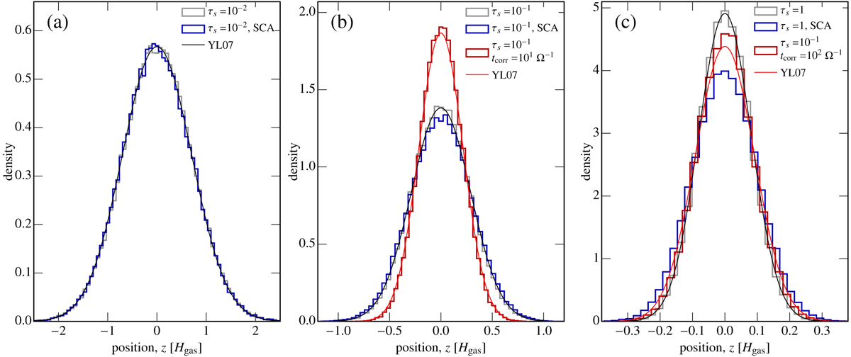
Vertical distribution for particles of different stopping times: τ_s = t_stopΩ = 10⁻² (panel a), 10⁻¹ (panel b), and 1 (panel c). Histograms plot the numerically obtained distributions with the stochastic equation of motion (SEOM; gray and red) and strong coupling approximation (SCA; blue) methods. Long t_corr runs are shown with red histograms (the t_corr = 10² Ω⁻¹, τ_s = 0.1 run is displayed in panel c). Thin curves gives the normal distribution with the scaleheight of Eq. (15) (Youdin & Lithwick 2007). Note the different scaling among the panels.