| Issue |
A&A
Volume 612, April 2018
|
|
|---|---|---|
| Article Number | A102 | |
| Number of page(s) | 16 | |
| Section | Interstellar and circumstellar matter | |
| DOI | https://doi.org/10.1051/0004-6361/201730837 | |
| Published online | 04 May 2018 | |
An X-ray survey of the central molecular zone: Variability of the Fe Kα emission line★
1
APC, Université Paris Diderot, CNRS/IN2P3, CEA/Irfu, Observatoire de Paris, Sorbonne Paris Cité,
10 rue Alice Domon et Léonie Duquet,
75205
Paris Cedex 13, France
e-mail: This email address is being protected from spambots. You need JavaScript enabled to view it.
2
Space Sciences Laboratory, 7 Gauss Way, University of California,
Berkeley,
CA
94720-7450, USA
3
Service d’Astrophysique/IRFU/DRF, CEA Saclay, Bât. 709,
91191
Gif-sur-Yvette Cedex, France
4
Max-Planck-Institut für extraterrestrische Physik,
Giessenbachstrasse 1,
85748
Garching bei München, Germany
5
Department of Physics and Astronomy, University of California,
Los Angeles,
CA
90095-1547, USA
Received:
21
March
2017
Accepted:
30
November
2017
Abstract
There is now abundant evidence that the luminosity of the Galactic super-massive black hole (SMBH) has not always been as low as it is nowadays. The observation of varying non-thermal diffuse X-ray emission in molecular complexes in the central 300 pc has been interpreted as delayed reflection of a past illumination by bright outbursts of the SMBH. The observation of different variability timescales of the reflected emission in the Sgr A molecular complex can be well explained if the X-ray emission of at least two distinct and relatively short events (i.e. about 10 yr or less) is currently propagating through the region. The number of such events or the presence of a long-duration illumination are open questions. Variability of the reflected emission all over of the central 300 pc, in particular in the 6.4 keV Fe Kα line, can bring strong constraints. To do so we performed a deep scan of the inner 300 pc with XMM-Newton in 2012. Together with all the archive data taken over the course of the mission, and in particular a similar albeit more shallow scan performed in 2000–2001, this allows for a detailed study of variability of the 6.4 keV line emission in the region, which we present here. We show that the overall 6.4 keV emission does not strongly vary on average, but variations are very pronounced on smaller scales. In particular, most regions showing bright reflection emission in 2000–2001 significantly decrease by 2012. We discuss those regions and present newly illuminated features. The absence of bright steady emission argues against the presence of an echo from an event of multi-centennial duration and most, if not all, of the emission can likely be explained by a limited number of relatively short (i.e. up to 10 yr) events.
Key words: Galaxy: center / X-rays: general
Images of the Fe Kα emission as FITS files are only available at the CDS via anonymous ftp to cdsarc.u-strasbg.fr (130.79.128.5) or via http://cdsarc.u-strasbg.fr/viz-bin/qcat?J/A+A/612/A102
© ESO 2018
1 Introduction
The super-massive black hole (SMBH) at the centre of our Galaxy is accreting matter at a very low rate (Wang et al. 2013). Its associated source, Sgr A⋆, has a bolometric luminosity of only ~1036 erg s−1 which is more than eight orders of magnitude smaller than the Eddington luminosity of a SMBH of about 4 million solar mass (Boehle et al. 2016). It is highly variable in the infrared and experiences regular flares in X-rays, with a measured frequency of 1.1 per day above 1034 erg s−1 (Neilsen et al. 2013). The most dramatic changes in luminosity have been observed in X-rays with flux increases of more than two orders of magnitude compared to quiescent levels (Goldwurm et al. 2003; Porquet et al. 2008; Nowak et al. 2012; Barrière et al. 2014; Ponti et al. 2015b).
There are many phenomena that might have been caused by intense past periods of activity of Sgr A⋆ (see e.g. Ponti et al. 2013). An active phase a few million years ago could explain the existence of the huge Fermi bubbles extending 10 kpc above and below the Galactic centre (GC; Su et al. 2010; Zubovas et al. 2011; Guo & Mathews 2012) as well as the high level of ionization in the Magellanic stream observed by Bland-Hawthorn et al. (2013). Similarly, a large region located 2° below Sgr A⋆ filled with out-of-equilibrium plasma recombining for about 100 kyr was possibly produced by an energetic event at the GC about 100 kyr ago (Nakashima et al. 2013).
There are also numerous lines of evidence that Sgr A⋆ was much brighter in the more recent past. X-ray light echoes, mostly through the fluorescent Fe Kα line (Sunyaev et al. 1993; Koyama et al. 1996), have been observed in many locations within the 150 pc radius region surrounding Sgr A⋆ which is usually referred to as the central molecular zone (CMZ; Morris & Serabyn 1996). This gas is optically thick enough to efficiently scatter X-rays emitted by a source in the GC region.
Variations of the reflected emission have been observed in a number of distinct places in the CMZ: in the Sgr A complex (Muno et al. 2007; Ponti et al. 2010; Capelli et al. 2011, 2012; Clavel et al. 2013, 2014) as well as in Sgr B (Inui et al. 2009; Terrier et al. 2010; Nobukawa et al. 2011; Zhang et al. 2015). Besides establishing the nature of the emission as reflection, these rapid variations of the non-thermal X-ray emission from molecular clouds provide fundamental information on the temporal behaviour of the illuminating source.
The detailed light curves of the emission measured on small scales in the Sgr A complex with Chandra have so far revealed two distinct time constants in the region: a steady variation over 10 yr and a rapid rise and decay over a few years. Clavel et al. (2013) have concluded that at least two distinct events are currently propagating through the Sgr A complex; one has a typical duration of about 10 yr while the other is much shorter, perhaps 2 yr or less. Both are intense, with typical luminosities of the order of 1039 erg s−1 or more, and are likely originating in Sgr A⋆.
Understanding these centennial outbursts of Sgr A⋆ requires knowledge of the number and typical recurrence rate of events currently being reflected by the CMZ. If only reflections occurring within particular molecular complexes are considered, it is difficult to see the full picture: are all reflections due to the same events? Was there a long-term period of sustained activity, or conversely, were there multiple short events (see e.g. Ryu et al. 2013)? To answer these questions, it is necessary to have a global view of variations in the region.
To achieve this, XMM-Newton performed a deep (640 ks) scan of the CMZ at the end of 2012. A comparison with older data and in particular with a shallower survey performed in the early mission in 2000–2001, makes it possible to assess the level of variation in the whole region.
We present in this paper a systematic comparison of these two datasets. Following the approach of Clavel et al. (2013), we determine the 6.4 keV line flux in 1′ pixels over the entire CMZ at various epochs to test for variability in a systematic manner. We show that most of the regions that are bright in this line have experienced significant variation over the 12 yr of XMM-Newton observations.
Examining the variable emission from a number of molecular complexes, we confirm the presence of variations characterised by two distinct time constants observed in various parts of the Sgr A complex; we report the first signature of a decrease of the Fe Kα flux observed in Sgr C and discuss the characteristic duration of the associated event; we also provide evidence suggesting an increase of the emission from the Sgr D complex between 2000 and 2012. We report the sudden illumination of a large elongated structure covering more than 25 pc in projection. Finally, we argue that these findings support the idea that almost all of the Fe Kα emission can be attributed to relatively short-duration events (i.e. up to 10–20 yr) and that no long-term sustained activity is required to explain the observations.
2 XMM-Newton observations and data analysis
Since its launch in 1999, the XMM-Newton satellite has been regularly monitoring the inner GC region, mostly focusing on Sgr A⋆ and on pointed observations of bright sources, but also through two more extended scans covering about 2° in longitude and 0.5° in latitude, performed in 2000–2001 and in 2012. In particular, the 2012 scan uniformly covers the sky between l = −0.8° and l = +1.5° with 16 pointings of 40 ks each, evenly separated by 7.8′ (bottom panel in Fig. 1).
These two scans as well as a large number of observations pointed within 1° were used to produce complete maps of the X-ray emission in the CMZ (Ponti et al. 2015c). We use here the same dataset which yields 101 observations with data from at least one EPIC detector, and a total of 285 single-exposure images.
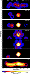 |
Fig. 1 Time exposure maps for the 7 epochs in which the XMM-Newton data have been grouped (in units of seconds, with 2.5″ pixel size, and in Galactic coordinates) after applying the exposure time cuts discussed in Sect. 2.1. The darker circular regions correspond to the point sources that have been excluded (see the list in Table A.1). The MOS1 and MOS2 exposures have been rescaled to take into account the different MOS and PN effective areas in order to create the PN-equivalent exposure mosaics shown here. |
2.1 Imaging analysis
The selected dataset was analysed in a uniform way using the XMM-Newton Extended Source Analysis Software (ESAS; Snowden et al. 2008)included in the version 12.0.1 of the XMM-Newton Science Analysis Software (SAS). For each available exposure, calibrated event lists were produced using the SAS emchain and epchain scripts and periods affected by soft proton flaring were excluded using ESAS mos-filter and pn-filter. The quiescent particle background was obtained using filter wheel closed event lists provided by the ESAS calibration database.
Since the goal of our study is to follow the Fe Kα variability across the CMZ through a uniform analysis and within different epochs, we based our investigation on the imaging (rather than the spectral) analysis of the XMM-Newton data, which allows us to simultaneously study large regions, on different angular scales, and to follow the morphological changes of the emission with time. Therefore, for each instrument and observation, count, background and exposure time maps were produced in the 4.7–6.3 keV continuum energy band and in two narrow bands centred at 6.4 and 6.7 keV (ΔE = 160 keV) in order to produce background- and continuum-subtracted images at 6.4 keV. The continuum band was chosen in order to have sufficient signal statistic in an energy range not affected by the presence of emission lines from the GC or instrumental background lines. The continuum underlying the 6.4 keV emission line was estimated using the flux of the 4.7–6.3 and 6.62–6.78 keV energy bands and assuming a simple model to represent the X-ray emission spectrum: a power law with photon index Γ = 2 (modelled with powerlaw in Xspec) and a plasma component (apec) with temperature kT = 6.5 keV and solar abundances. Both components were absorbed by a foreground column density of NH = 7 × 1022 cm−2 (Ponti et al. 2015c). This allows allows a (background- and continuum-subtracted) net count map to be produced at 6.32–6.48 keV for each instrument and each observation. In order to obtain the total net counts included in the 6.4 keV line, we applied an efficiency correction to the 6.32–6.48 keV net count map. This correction is required to correct for leakage of events outside the selected band because of energy dispersion. The probability that the energy of a line photon is measured in the energy range is obtained from the canned redistribution matrices1.
The same correction was also applied to the 6.62–6.78 keV flux map before using it to estimate the continuum contribution at 6.4 keV. For this band, the correction is applied only to the fraction of flux that is expected to be contained in the line following the model and parameters considered here (i.e. 82% of the total 6.7 keV flux, while the rest is continuum emission).
To be able to combine images from the different instruments, the exposure time maps were renormalized taking into account the differentefficiencies of the three EPIC detectors. In addition, circular regions corresponding to some of the brightest transient or persistent X-ray point sources have been excluded (see Fig. 1 and Table A.1). In particular for the transient sources, the corresponding region was excluded only when the source was found to be in outburst.
Each net count and exposure time map was then reprojected with the Chandra tool reproject_image_grid to a common, specified grid. We produced reprojected maps with different spatial resolutions using pixel sizes of 2.5″ and 1′. To produce the final mosaics, summed count and summed exposure time maps were produced and the intensity maps were computed. In order to exclude the less exposed regions, for example, the image borders, which might induce spurious results in the variability analysis, we removed: (1) in each observation, the pixels with exposure times less than 10% of the maximum in that specific observation, and (2) in each mosaic, the pixels with exposure times less than 20% of the median in that specific mosaic.
The variability analysis presented in the following is mostly based on the final mosaic images at 6.4 keV produced by grouping the data taken within the years 2000–2001, 2002–2003, 2004–2005, 2006–2007, 2008–2009, 20112, and 2012. Two mosaics were created for 2012, one with all data collected that year (for comparison with the other epochs) and the other with only the 16 pointings of the survey (for comparison only with the 2000–2001 scan). Even though the selected time periods have quite different exposure coverage, most of the regions of interest for our study are covered for a minimum of 3–4 epochs (e.g. Sgr B, Sgr C, Sgr D) and up to 7 epochs for the 15′ radius around Sgr A⋆ (Fig. 1).
2.2 Comparison of the imaging and spectral fluxes
In order to validate the results obtained from the imaging analysis, we compared the Fe Kα fluxes measured with our procedure to those obtained with the standard ESAS spectral analysis for some specific regions. For this purpose, we selected four circular regions of different surface brightness within 12′ of Sgr A⋆. In particular, two low-brightness regions with a radius of 164″ were chosen at the west of Sgr A⋆ (regions labelled “north” and “south”), while a high-brightness region with the same radius was centred to the south-east of Sgr A⋆ (“east”), including the bright cloud G0.11–0.11. At intermediate brightness values, a region of 102″ radius was selected that includes the Arches cloud and cluster (“Arches”).
For each time period and each region, the spectra of all observations and from all instruments have been fitted simultaneously with the model also used to estimate the continuum emission underlying the 6.4 keV line in the imaging analysis (Sect. 2.1), in order to have fully comparable results. Considering that this model is not necessarily adapted to each region, we find a good agreement between the two methods, with an average difference of the imaging versus spectral fluxes of 3%, − 10%, 8%, and − 2% for the north, south, east, and Arches regions, respectively (Fig. 2). In particular, the most extreme outlier for the Arches region corresponds to the 2006–2007 period when the increased 6.7 keV line due to a flare of the Arches cluster contaminates the 6.4 keV line in the spectral fitting (Capelli et al. 2011).
About 60% of the tested regions have their 6.4 keV fluxes consistent within 10% with the spectral extraction and all but one are consistent within 15%. Since the level of background emission is also varying with longitude in the CMZ, we also compared the fluxes in more distant regions. In the region G0.66–0.03 (ℓ ~ 0.7°, see Table A.2), the fluxes are consistent within 7%, while in the weak and distant region Sgr D-Core (ℓ ~ 1.1°, see Table A.2), they are consistent within 16%. We therefore conclude that our systematic uncertainty on the flux value resulting from imagery is at the level of 10–15%.
We also evaluated the impact of the chosen plasma models to extract the 6.4 keV line flux. In particular, changing the abundance of the kT = 6.5 keV apec to 2 as was found by, for example, Capelli et al. (2012), we found typical flux variations inferior to 3% well below the level of systematics discussed above.
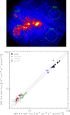 |
Fig. 2 Comparison of the Fe Kα fluxes extracted from the mosaic images with those obtained from the spectral fitting for the four test regions within 12′ of Sgr A⋆ visible in the inset. The data have been grouped into eight periods as described in the text (with the 2012 data split between the March and autumn observations). The dashed line indicates where regions with the same fluxes from imaging andspectral analysis should lie and the dotted lines represent the 10% dispersion around it. |
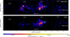 |
Fig. 3 Background- and continuum-subtracted intensity maps of the inner GC region measured by XMM-Newton at 6.4 keV in 2000–2001 (top) and 2012 (bottom). The maps are in units of ph cm −2 s −1 pixel−1, with 2.5″ pixel size, and smoothed using a Gaussian kernel of 5 pixels radius. The dotted square regions are discussed in more detail in Sect. 4. |
3 Variability of the Fe Kα line
Thanks to the extensive XMM-Newton coverage of the CMZ we are for the first time able to follow the variations of the Fe Kα line emission over 13 yr simultaneously in several molecular complexes. Figure 3 presents the Fe Kα intensity maps of the2000–2001 and 2012 XMM scans (which cover similar sky areas) with a pixel size of 2.5″ ×2.5″. The variability of the 6.4 keV emission is clearly visible all over the central degree. To quantitatively study variability on large scales and to produce light curves of specific regions we used maps with a coarser binning of 1′ × 1′ pixels, which provide a larger number of counts per pixel.
We first compare the 2000–2001 and 2012 scans; then using all mosaics we determine regions of the CMZ which have 6.4 keV emission significantly varying over the 12 yr period considered here. Finally in Sect. 4, we provide light curves of the Fe Kα emission and discuss its evolution for most of the 6.4 keV bright structures in the CMZ.
3.1 Comparison of the 2000–2001 and 2012 scans of the CMZ
When comparing the global 6.4 keV maps obtained in 2000–2001 and 2012, it is already evident at first glance that a global decrease is observed between these two epochs (see Fig. 3 and Ponti et al. 2014). The total 6.4 keV emission within a common rectangular area of 19 × 112 arcmin2 size decreased from Ftot(2000–2001) = (1.76 ± 0.03) × 10−3 ph cm−2 s−1 to Ftot(2012) = (1.507 ± 0.009) × 10−3 ph cm−2 s−1, corresponding to a total decrease of 14%, which is marginally significant given the typical systematic error on the Fe Kα line flux obtained with the imaging approach. The average surface brightness over the same area decreased from Btot (2000–2001) = (8.6 ± 0.1) × 10−7 ph cm−2 s−1 arcmin−2 to Btot (2012) = (7.36 ± 0.04) × 10−7 ph cm−2 s−1 arcmin−2. These averaged values may be smoothing out strong variations occurring over a small fraction of the region.
In order to quantify the significance of the variations in the different regions, we applied to the 1 arcmin intensity maps the false discovery rate (FDR) technique. This method (whose application to astrophysical data is described by Miller et al. 2001) allows us to compare data against a model hypothesis while a priori controlling the number of false rejections, rather than setting a confidence limit as is done in standard procedures. The FDR has the advantage of providing a comparable rate of correct detections but fewer false detections than other common statistical methods.
Within the rectangular area common to the two scans, we retained only pixels that were exposed during both scans and where the 6.4 keV emission was detected at ≥3σ in at least one of the two epochs. As a result, 1092 pixels are selected in which we can test for variability. A false rejection rate of 10% has been chosen in order to obtain a good balance between the number of false and true detections. We also verified with a rate of 5% that the regions detected to vary are substantially the same as for 10%. Out of the 1207 pixels tested, 60 show significant variability, representing 5% of the total. Of the variable pixels, the large majority (80%) are found to decrease from 2000–2001 to 2012.
While they represent a small fraction of the total number of pixels, these variable pixels are in fact all among the brightest ones. If we limit the sample to the pixels having a brightness larger than 3 × 10⁻⁶ ph cm−2 s−1 arcmin−2 in at least one of the two scans, we find that the majority (70 out of 105) of the bright pixels vary significantly (beyond 2σ, see Fig. 4). The significantly variable pixels are therefore the brightest. The numerous pixels which do not show significant variation are, of course, not necessarily constant. We lack the sensitivity to observe variations in fainter pixels mainly because the first survey is not deep enough. The relevant point here is that most, if not all, bright pixels do vary on a 10 yr timescale.
When limiting the comparison to the bright Fe Kα pixels, a larger decrease by more than 30% is detected, the average surface brightness of these pixels varying from Bbright(2000–2001) = (46.9 ± 0.9) × 10−7 ph cm−2 s−1 arcmin−2 to Bbright(2012) = (31.7 ± 0.3) × 10−7 ph cm−2 s−1 arcmin−2.
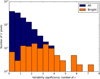 |
Fig. 4 Histogram of the significance of variations of Fe Kα line emission in 1′ pixels between the 2000–2001 and 2012 surveys. Nearly all pixels with a brightness larger than 3 × 10⁻⁶ ph cm−2 s−1 arcmin−2 are found tovary. |
3.2 Multi-year variability
To characterise localised variations in the whole CMZ region over several years, we performed a systematic analysis following the method presented by Clavel et al. (2013). We made use of the Fe Kα mosaic images grouped by periods of 2 yr and extracted a light curve for each pixel of 1′ size (see Sect. 2.1). Each pixel’s light curve was fitted with both constant and a linearly varying intensity model using χ2 statistics to provide rejection probabilities for both models. These resulting probabilities were then combined on scales of 2 × 2 arcmin2. The latter step has the advantage of emphasising the results on more extended regions showing similar trends, while on the other hand it makes it difficult to estimate a precise fraction of variable regions over the whole survey area, as a one-to-one correspondence between the initial maps and the significance map is lost. To limit false variability detections, we corrected the probabilities for the number of trials, which is given by the total number of pixels in the map for which variability can be detected3. In Fig. 5 the results of the variability analysis are presented for this selection of pixels with sufficient statistics to be able to detect a minimum level of variability.
A significant deviation from a constant fit is observed in several large regions, which are associated with the Sgr A, B, and C complexes. The structures in Sgr B, as well as most of the Sgr A complex, present the most significant variations (≥ 4σ post-trial). The large majority of the variable pixels can be clearly associated with either well-known bright molecular clouds, or to fainter molecular clumps. We note that the variable pixels just to the Galactic west of Sgr A⋆ are most likely due to residual variability of the neutron star X-ray binary AX J1745.6-2901, not completely removed during the exposure cut (see e.g. Ponti et al. 2015a).
In order to have an indication of whether an increase or a decrease of emission is observed, the map giving the slope of the linear fit at each position is reported in Fig. 5 (bottom panel). Although the observed variations are, for the large majority, linear, non-linear variability has been significantly detected on arcmin scale in the Sgr A complex (see centre panel of Fig. 5), in particular in MC1 and MC2, in the Bridge, around the Arches cluster, and in the south-east part of G0.11–0.11 (the regions are detailed in Table A.2 and in Sect. 4.1). This confirms the results obtained with Chandra observations from 1999 to 2011 on smaller scales for the Bridge as well as MC1 and MC2 clouds (Clavel et al. 2013). Therefore, on the observed scales, there does not seem to be strong indication for non-linear variability except for that already reported in the Sgr A complex by Clavel et al. (2013). This is likely due to the more limited time sampling outside Sgr A (see Fig. 1).
In some regions, the variability is not significantly detected by this kind of analysis on arcmin scales; for example, the northern part of the Sgr C complex and the G0.24–0.17 filamentary region (see later). This is due to the low surface brightness of these regions and to the fact that propagation of the emission is observed here rather than an on-off behaviour. Indeed, when applying the same kind of analysis but combining the χ2 probabilities on 3 × 3 arcmin2 scales, the significance of rejection of a constant fit increases to ~3σ for the northern region of Sgr C. However it still remains negligible for G0.24–0.17 because of its elongated structure.
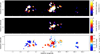 |
Fig. 5 Maps resulting from the variability study of 7 periods from 2000 to 2012, using a 1′ pixel size. Top: significance of rejection for a fit with a constant-intensity model applied to each bin light curve, and after performing aχ2 smoothing (see text for details). Centre: same as top panel but applying a linear fit. Bottom: slope of the linear fit for the pixels for which variability can be detected and with non-zero significance shown in the top panel. |
4 Variability in specific regions
We discuss here variability of specific regions. We consider most of the regions that have already been the subject of a number of studies as well as a few others revealed in this analysis. We refer to Table A.2 for details and relevant references. All errors shown on the light curves are 1σ errors (68% confidence level).
4.1 Sgr A: two distinct timescales
Figure 6 shows the evolution of the Fe Kα emission in the whole Sgr A complex. If the global flux does not vary significantly, variability on small scales is very strong. Such variability has previously been detected in several regions with XMM and Chandra (Muno et al. 2007; Ponti et al. 2010; Capelli et al. 2011; Clavel et al. 2013, 2014). Since the complete XMM data set covers a larger sky area and longer time period, we are able here to follow the evolution of known varying regions and detect variability from additional molecular structures.
In particular, a complex variability behaviour is detected north of the MC1 and bridge clouds, in a region corresponding to two molecular filaments that seem to connect these regions to the Arches and to the DX clouds. These filamentary structures correspond to molecular matter in the −35–5 and 35–65 km s−1 ranges, respectively (Tsuboi et al. 2011), and therefore similar velocity ranges as the MC1 and Arches cloud for the former and the Bridge (Br1 and Br2 regions) for the latter (see Fig. 6). The Arched filaments show globally increasing emission, while the 6.4 keV emission of the western filament is decreasing (see Fig. 5). We extracted the light curves of these regions in two elliptical regions, named G0.02+0.01 and G0.09–0.02 (see Table A.2). The former shows a steady 25% linear flux decrease over the 12 yr, while the flux of the latter increases by more than 35% in the same time period with a constant flux rejected at nearly 5σ (see last panels of Fig. 7).
The Arches and DX clouds themselves are detected to have decreased during the 12 yr separating the two surveys. A spectral analysis of the Arches region variability was performed and described in Clavel et al. (2014). Our new results are in full agreement and we refer to this paper for a light curve of the region. The DX light curve (Fig. 7, last row second panel) shows a clear smooth decrease (rejection of a constant fit at 6.4σ) and no indication for a peak in 2004 is found, contrary to what was reported by Capelli et al. (2011). To ensure that the discrepancy is not caused by the different time binning of the data, we extracted a light curve using only the observations and instrument exposures used by Capelli et al. (2011) and grouping them in the same way. We found flux points consistent with those obtained by Capelli et al. (2011) within the quoted uncertainties, but the overall light curve is smoother with no hint of a peak in August/September 2004, and thus not supporting the hypothesis of a strong flux increase in 2004.
On the other hand we can confirm that not only is the propagation of the signal, which has already been observed in several regions of Sgr A, still on-going in the Br1, Br2, MC1 and MC2 clouds, but that it is also observable in other regions. In particular, the emission displacement is visible further away from Sgr A⋆, that is, within the G0.11–0.11 cloud, where the two brightest regions of 2000–2001 appear to be shifted towards the Galactic east and to have significantly dimmed in the 2012 map (Figs. 3 and 6). Moreover, we detect for the first time here the variability at 6.4 keV of the region south of Br1/MC2, named G0.04–0.13 in Clavel et al. (2013). The light curve extracted from this region over the 12 yr shows a smooth increase and a plateau (Fig. 7, last row middle panel). When looking on smaller scales (Fig. 6), one can observe the propagation of the 6.4 keV emission along a structure extending towards the south of the Bridge. The CS emission of the molecular counterpart of this region is faint and is not visible in the last panel of Fig. 6.
As predicted by Clavel et al. (2013), the large-scale emission of MC1 has started to decrease, following a peak in 2011. Within the elliptical region of Fig. 6, the flux in 2012 has decreased by about 15% with respect to that in 2011 and the 12 yr light curve now reveals significant variability in this cloud even on arcmin scales (Fig. 7). A very thin filament (0.2 × 8 pc2) was detected within Br2 in the 2011 Chandra observations during which it showed a sharp emission increase consistent with a two-year variation (Clavel et al. 2013). It is also detected by XMM in 2011 and its flux is observed to be decreasing in 2012 (by about 20% compared to 2011), supporting the hypothesis that it is reflecting a short flaring event (rejection of a constant fit at 13σ; Fig. 7, first row, right panel). The corresponding region is not shown in Fig. 6 but is detailed in Table A.2.
Molecular features highlighted by CS emission in the 40–70 km s−1 range all show strong variability with a typical timescale of about 1–2 yr (see the Br1, Br2 and 2011 filament light curves; the case of the faint region G0.09–0.02 is less clear). As shown by Clavel et al. (2013), they must have been illuminated by a short event with a maximum duration of ~2 yr. All the other 6.4 keV emitting regions display a smooth evolution over the 12 yr covered and are likely due to a longer-duration (typically 10 yr) event.
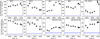 |
Fig. 7 Fe Kα light curve of the illuminated clouds in the Sgr A complex (regions indicated in Fig. 6). The blue band shows the level of background line emission estimated in a large region below Sgr A⋆. All errors shown on the light curves are 1σ errors (68% confidence level). |
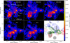 |
Fig. 6 Fe Kα flux images of the Sgr A complex in the period 2000–2012. The dotted lines mark the regions discussed in the text and whose light curves are extracted. The bottom right panel shows the same regions, as grey ellipses, compared to the various structures of the molecular complexes traced by CS shown as solid lines (blue −20–10 km s−1, red 10–40 km s−1 and green 40–70 km s−1). Short timescale (≲2 yr) variations are mostly visible in structures in the last velocity range. |
4.2 Sgr B: a strong flux decay and newly illuminated structures
The reflected emission in the Sgr B region is known to decay both in the Fe Kα line and hard X-ray continuum (Inui et al. 2009; Terrier et al. 2010; Nobukawa et al. 2011; Zhang et al. 2015); Figs. 8 and 9 clearly confirm this.
On large scales, the Sgr B circular region, which has a radius of ~16 pc at the GC distance enclosing most of the molecular complex, experienced a 6.4 keV line flux variation of a factor of 2 over approximately 10 yr. This variation is strongly statistically significant with a constant level rejected at 18σ. The total flux peaked in 2000–2001 at BSgr B(2000–2001) = (17.7 ± 0.7) × 10−7 ph cm−2 s−1 arcmin−2; it quickly dropped to BSgr B(2004) = (13.6 ± 0.3) × 10−7 ph cm−2 s−1 arcmin−2 and then decreased more smoothly to reach BSgr B(2012) = (9.0 ± 0.2) × 10−7 ph cm−2 s−1 arcmin−2. This emission is still a factor of 2 larger than the more diffuse emission that pervades the inner degree and is therefore clearly connected to the Sgr B molecular complex.
This behaviour at large scales masks more complex evolutions in smaller, localised regions. In the early measurements, most of the flux is due to a few very bright regions. The flux of these compact and dense cores decayed much more rapidly than the ten-year timescale observed in the larger region. If one excludes those cores, the large-scale brightness variation is less spectacular, as expected given the very large light-crossing time of the whole Sgr B2 complex. The small and bright cores having short light-crossing time, have emission light curves more closely reflecting the illumination light curve.
The 2 arcmin around the core of the Sgr B2 cloud were very bright in 2000–2001, with a brightness of BSgr B2 Core (2000–2001) = (50.4 ± 3.8) × 10−7 ph cm−2 s−1 arcmin−2, which fell by a factor of 4–5 over a duration of approximately 11 yr to BSgr B2 Core(2012) = (11.5 ± 0.6) × 10−7 ph cm−2s−1 arcmin−2, which is only slightly larger than the average brightness in the whole Sgr B region in 2012.
The huge column density of the core could also completely screen 6.4 keV emission as the echo propagates deeper into the core and produces a more rapid evolution than the actual illumination duration (e.g. Walls et al. 2016). In particular, we note that NuStarobserved significant hard X-ray emission from the dense cores in 2013, most likely because of multiple scatterings in very high opacity regions (Zhang et al. 2015).
A similar rapid decay is observed in the G0.74–0.10 region (Nobukawa et al. 2011) where the flux is diminished by a factor of about 5 from BG0.74-0.10(2000–2001) = (45.9 ± 4.8) × 10−7 ph cm−2 s−1 arcmin−2 to BG0.74-0.10(2012) = (10.7 ± 0.7) × 10−7 ph cm−2 s−1 arcmin−2, again only slightly larger than the average brightness in the whole Sgr B region. The flux of region G0.50–0.11, discovered by Nobukawa et al. (2008), is also declined by nearly a factor of 3 to reach a similar flux level.
Finally, the 2012 survey saw the appearance of two new illuminated regions. The first one, G0.66–0.13, was first reported by Zhang et al. (2015). It is clearly visible on the maps (see Figs. 3 and 8) and its light curve (fourth panel of Fig. 9) shows an increase with a 3.1σ statistical significance level. NuStar observations suggest it was already dim in 2013 (Zhang et al. 2015), suggesting that a short duration event might be propagating in the region. The second region G0.56–0.11 has a flux level consistent with the background, except in 2012 where it reaches (14.0 ± 0.8) × 10−7 ph cm−2 s−1 arcmin−2, rejecting a constant flux by 7σ.
Further observations and studies of variations of these regions will be necessary to constrain the number and duration of the events propagating in the Sgr B complex.
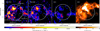 |
Fig. 8 Fe Kα images of the Sgr B complex. The right panel shows the total gas column density measured by Herschel (Molinari et al. 2011). |
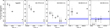 |
Fig. 9 Fe Kα light curves of the Sgr B complex integrated over the regions indicated in Fig. 8. All errors shown on the light curves are 1σ errors (68% confidence level). |
4.3 Sgr C: decrease and displacement
ASCA and more recently Suzaku have shown that several regions within the Sgr C molecular complex emit at 6.4 keV (Murakami et al. 2001b; Nakajima et al. 2009; Ryu et al. 2013). Only limited variability had been reported by Ryu et al. (2013) for the X-ray clump named C1 between two Suzaku observations (+8% at 2.9σ level), and apossible positional shift compared to past ASCA images was suggested (Nakajima et al. 2009).
The data presented here show for the first time a highly significant and large variation of the Fe Kα flux in the Sgr C complex, detected with the same instruments and therefore free from cross-calibration issues. When the bulk of the 6.4 keV emission is integrated (elliptical region labelled Sgr C in Fig. 10), the total brightness is found to have decreased from BSgr C(2000–2001) = (12.7 ± 0.6) × 10−7 ph cm−2 s−1 arcmin−2 to BSgr C(2012) = (9.1 ± 0.3) × 10−7 ph cm−2 s−1 arcmin−2, that is, by 28%. A constant flux is excluded at the 5.5σ significance level. The amplitude of the variation is only a lower limit to the true amplitude, since the large-scale background level in the vicinity of Sgr C (and outside the bright clumps discussed here; see Fig. 10) is on average about Bbkg, Sgr C ~ 6 × 10⁻⁷ ph cm−2 s−1 arcmin−2 (Fig. 11).
The actual pattern of the variations is complex. Light curves of smaller-scale regions are presented in Fig. 11. These regions, described in Table A.2, are taken from Nakajima et al. (2009) and Ryu et al. (2013), and we add a new one we call C4 following the nomenclature used in the latter paper. We find no significant emission from the small clump M359.38–0.00 in excess of the background. The large region called C3 shows no significant variations. Regions C2 and C4 both decrease significantly, with a constant flux rejected at 4.7 and 5.8σ, respectively. Their brightnesses have decreased by ~50% from 2000 to 2012.
The structure called C1 does not show a significant flux variation over the 12 yr, with a brightness measured at (15.3 ± 0.7) × 10−7 ph cm−2 s−1 arcmin−2 in 2012. Yet, time-resolved images show a clear positional displacement of the 6.4 keV centroid for the C1 clump (Fig. 10). To quantify the displacement, we determined the position of the centroid at each period by computing the barycenter of the emission in the C1 region from the flux maps shown in Fig. 10. In 2012, the centroid is displaced by about 1.6′ from the Sgr A⋆ direction compared to its position in 2000–2001. When comparing the centroid positions to the molecular matter distribution (rightmost panel of Fig. 10), one can see the 6.4 keV emission moving along a rather filamentary structure, which is visible in the velocity range from −80 to −60 km s−1 in the HCNmap. Besides, while not perfectly aligned with the molecular matter, the Fe Kα emission in C1 is elongated in a similar direction. All this suggests we are observing the propagation of the illuminated region along a dense matter structure. This is the first time this phenomenon is observed at negative longitudes and it is consistent with Sgr A⋆ as the illuminating source. We can also use this propagation to constrain the duration of the illumination; see Sect. 5.
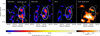 |
Fig. 10 Fe Kα maps of the Sgr C complex for three periods of XMM-Newton observations (first three panels from the left) and Mopra HCN map integrated over the − 80 to − 60 km s−1 velocity band for the same region (right panel). The yellow, green, and cyan dots give the position of the centroid of the emission in the C1 region in 2000−2001, 2006−2007 and 2012, respectively. A displacement of 1.6′ of the emission in a direction similar to that of the molecular feature is visible. The Fe Kα maps are in units of ph cm−2 s−1 pixel−1, with 2.5″ pixel size, and smoothed using a Gaussian kernel of 8 pixels radius. The solid line region labelled Sgr C includes the bulk of the Fe Kα bright clumps, while the smaller regions reported by other papers plus the C4 clump newly labelled here are shown in dotted lines. |
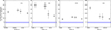 |
Fig. 11 Fe Kα light curves of the Sgr C complex (circles) integrated over the regions indicated in Fig. 10. The blue band indicates the level of background emission measured in a large region defined in Table A.2. All errors shown on the light curves are 1σ errors (68% confidence level). |
4.4 Propagation in M359.23–0.04
We also investigate the region M359.23–0.04 that was discovered by Nakashima et al. (2010) during a Suzaku observation in 2008. It was found to be coincident with two molecular features one appearing in the velocity range −140 to −120 km s−1 and a second in the range −20 to 0 km s−1. Because of its distance to Sgr A⋆ Nakashima et al. (2010) argued that the origin of the illumination could also be the nearby 1E 1740.7–2942 (6′ in projection).
M359.23–0.04 is visible only in our 2000–2001 and 2012 maps. An elongated feature is visible and is found to be well aligned with the molecular matter traced by CS in the velocity band −140 to −120 km s−1 (see Fig. 12). The latter is therefore the likely matter counterpart of this reflection nebula. The nebula appears weakly variable in the systematic search presented in Sect. 3.2 but an apparent displacement of the emission towards the Galactic west is suggested by the Fe Kα maps (Fig. 12). This displacement follows the distribution of dense gas4.
To quantify this, we define two regions encompassing the two blobs of the molecular structure which are well exposed with XMM and we extract their 6.4 keV flux (see Table A.2). The brightness of the first blob decreases from (10.5 ± 1.2) × 10−7 to (6.6 ± 0.6) × 10−7 ph cm−2 s−1 arcmin−2 (a 2.8σ variation), while the brightness of the second, located farther away from Sgr A⋆, increases from (7.4 ± 1.2) × 10−7 to (12.1 ± 0.9) × 10−7 ph cm−2 s−1 arcmin−2 in the same period (a 3.1σ variation). Although the statistical significance of the variations is not very strong, it is tempting to interpret this as the light echo propagating along a molecular structure, as in the case of the C1 feature discussed above. This positional shift towards the Galactic west would be consistent with an origin of the echo in the inner regions of the GC rather than in the nearby binary. In that case, as was shown by Nakashima et al. (2010), a ~1039 erg s−1 flare from Sgr A⋆ could explain the observed luminosity. Further deep observations of the region are needed to convincingly validate this interpretation.
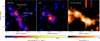 |
Fig. 12 Left: Fe Kα maps centred at the position of the M359.23–0.04 structure during the 2000–2001 and 2012 XMM-Newton observations. The maps are in units of ph cm−2 s−1 pixel−1, with 2.5″ pixel size, and smoothed using a Gaussian kernel of 15 pixels in radius. Right: CS(1–0) map integrated in the −140 to −120 km s −1 velocity band. |
4.5 Sgr D: reflection in a distant cloud and weak evidence for variation
Sgr D is located at the Galactic east of Sgr A⋆ at a projected distance of about 180 pc and this more distant molecular structure is also less massive than Sgr A, B or C. Therefore, this cloud isonly intercepting a very limited fraction of the signal emitted by the central source, making detection and variability studies of its 6.4 keV emission very challenging. Before our deep 2012 observation, Sgr D had been observed with BeppoSAX, with XMM (in 2000 and 2005) and with Suzaku (in 2007). These earlier observations revealed multiple sources of X-ray emission in the region (Sidoli et al. 2001, 2006; Sawada et al. 2009; Ponti et al. 2015c), including an extended 6.4 keV clump (Ryu 2013). In 2007, this extended feature had a surface brightness of I6.4 keV = (2.7 ± 0.3) × 10−7 ph cm−2 s−1 arcmin−2 (unabsorbed, corresponding to a measured brightness of ~ 2.2 × 10⁻⁷ ph cm−2 s−1 arcmin−2 and a possible X-ray nebula origin was then mentioned (Ryu 2013).
Making use of the 2012 observations covering Sgr D, we confirm this result with a clear detection of its 6.4 keV emission with XMM. The bulk of the Fe Kα emission is contained in the elliptical region we call “Sgr D core” (see Fig. 13 and Table A.2). This emission is found to be coincident with a molecular feature in the CS data in the velocity range 50 to 70 km s−1. In 2012, it has a surface brightness of 3.8 ± 0.3 × 10⁻⁷ ph cm−2 s−1 arcmin−2. In 2000 and 2005, the 6.4 keV line emission of this region was compatible with the background level. However, the lower statistics of these earlier observations only provide weak evidence for the variability of Sgr D: the constant fit of the XMM light curve is rejected at a 3.3σ level and a linear fit is preferred over the constant one at a 3.7σ level5.
If this increasing trend is confirmed, Sgr D would be the furthest dense cloud from Sgr A⋆ (in projection) for which the Fe Kα emission and variability are observed, providing a constraint on the past event from Sgr A⋆ causing this echo to have occurred between 300 and 1100 yr ago (assuming that the line of sight distance of this cloud to the sky plane of Sgr A⋆ is less than 130 pc).
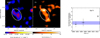 |
Fig. 13 Left: Fe Kα map centred at the position of Sgr D during the 2012 XMM-Newton observations. The map is in units of ph cm −2 s−1 pixel−1, with 2.5″ pixel size, and smoothed using a Gaussian kernel of 15 pixels radius. The region labelled Sgr D includes the bulk of the Fe Kα emission in the complex. Middle: CS map integrated in the velocity range 50 to 70 km s−1 showing the molecular counterpart of the 6.4 keV emission. Right: Fe Kα light curve of the Sgr D complex integrating over the region indicated on the maps. The blue band indicates the level of background emission. All errors shown on the light curves are 1σ errors (68% confidence level). |
4.6 G0.24–0.17: rapid illumination of a 25 pc-long structure
An interesting filamentary structure that appeared to be newly illuminated in 2012 (hereafter G0.24–0.17) is observed south-eastof the Sgr A complex. This feature has an elongated shape, roughly parallel to the Galactic plane (Fig. 14) which connects to the G0.11–0.11 cloud on its western edge. Looking into molecular tracer maps to search for a corresponding feature, we found a relatively faint filamentary structure of about 25 × 2 pc2 in projected size in the CS(1–0) maps obtained from the 7 mm Mopra survey of the CMZ (Jones et al. 2013), in the velocity range between 27 and 35 km s−1 (see Fig. 14). While not significant in itself, the very clear morphological match between the 6.4 keV and CS features strongly suggests the latter is real and is the molecular counterpart of the Fe Kα line emission observed by XMM-Newton in 2012.
We selected a polygonal region containing most of the CS line and the 2012 Fe Kα line emissions of the filament and computed the total flux at different epochs (Fig. 14). A constant fit of this light curve is rejected at 3.9σ. For each epoch we also compared the surface brightness of the filament with that of the background within the same mosaic image, estimated over a circular region southof Sgr A⋆, free of bright 6.4 keV emission. In the 2012 mosaic, a total brightness of (12.5 ± 0.5) × 10−7 ph cm−2 s−1 arcmin−2 is measured compared to a 2000–2001 brightness of(7.8 ± 1.2) × 10−7 ph cm−2 s−1 arcmin−2, which is compatible with the average background within 2σ (Fig. 14). In addition, the brightest emission in 2000–2001 seems to rather come from across the north-east border of the polygonal region. This suggests that the illumination propagated through the 25 pc-long filament within less than the 12 yr separating the two surveys; another case of superluminal echo. This places strong constraints on the filament location and orientation with respect to the illuminating source. Furthermore, the faintness of the CS counterpart indicates that the column density of this molecular structure is small and hence that the luminosity of the source must be large. We discuss these constraints further in the following Section.
Finally, we note that a complex region of 6.4 keV emission is also visible in 2012 around − 0.10° < b < −0.15°, and 0.15° < ℓ < 0.35°; see Fig. 14. The flux variation of this feature has positive slope in Fig. 5. This suggests that the illumination is propagating farther than the Sgr A molecular complex.
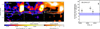 |
Fig. 14 Left images: Fe Kα maps centred at the position of the G0.24–0.17 filament during the 2000–2001 and 2012 XMM-Newton observations. The maps are in units of ph cm−2 s−1 pixel−1, with 2.5″ pixel size, and smoothed using a Gaussian kernel of 8 pixels in radius. Centre: Mopra CS(1–0) map integrated over the 27–35 km s−1 velocity band. Right: Fe Kα light curve of the G0.24–0.17 filament. The blue band indicates the level of background emission measured in a circular region south of Sgr A⋆. All errors shown on the light curves are 1σ errors (68% confidence level). |
5 Discussion
5.1 Timescales of variations
We have shown, in Sect. 3.1, that most bright regions have significantly varied over the 12 yr separating the two XMM surveys. In particular, very few regions that were bright during the 2000–2001 scan have a compatible flux in 2012. We can therefore conclude that typical timescales in these regions are of the order of or shorter than 10 yr. Those regions are not illuminated by a century-long steady event; if they were we would have observed more stable flux levels.
We also confirm the existence of two distinct timescales in the variations observed in the Sgr A complex as was first noted by Clavel et al. (2013). These patterns are observed in distinct molecular structures which are located in different velocity ranges. The rapid variations are limited to structures in the 40–70 km s−1 velocity range (the so-called Bridge), while the longer variations (10 yr timescale linear variations) are visible mostly in molecular features visible in the −20 to 10 and 10 to 40 km s−1 ranges (see Fig. 6). If, as suggested by Churazov et al. (2017b), every Fe Kα bright cloud is illuminated by only one short event, they all should lie in a very limited range of positions along the line of sight. This seems unlikely. Indeed, while one can assume that some of the clouds are interacting, we note that the molecular structures, which represent most of the mass in this direction, are distributed over a broad range of velocities and cover more than 20 pc in projected distance. Therefore we consider that several events are required to explain the observations.
The variations observed in the Sgr B complex are rather rapid. The bright regions, Sgr B2 core and G0.74–0.10, have decayed by a factor of 4–5 in 12 yr and are now at a level similar to the average brightness level of the Sgr B complex. This decrease is much more rapid than what is observed in most regions of the Sgr A complex, such as MC1 and MC2, which have similar or smaller physical sizes. This might suggest, at first, that these clouds are illuminated by a short flare of a few years in duration, but absorption and propagation effects can also strongly modify the light curve. Sgr B2 is the most massive cloud in the Galaxy, with a peak column density beyond 1024 cm−2 (Protheroe et al. 2008) and is therefore opaque at 6.4 keV. In this energy range, we can only see reflection from the skin of the densest regions, whereas hard X-rays can still escape from the cores, as seen by NuSTAR (Zhang et al. 2015). The 6.4 keV light curve of less dense clouds in the region should follow more closely the illumination. In that respect, we note that the future evolution of the newly illuminated features, G0.66–0.13 and G0.56–0.11, will be very beneficial for constraining the illuminating event light curve. NuSTAR observations carried out in 2013 suggest the flux of the former has already decreased (Zhang et al. 2015).
5.2 Duration of the illumination in Sgr C
The overall emission in the Sgr C complex is decreasing. In particular, regions C2 and C4 show a significant and rapid decrease. The case of region C1 is more subtle: if the total flux does not show any significant variation, the centroid of the emission is moving in a direction following the elongated molecular structure shown in Fig. 10. We argued that this is consistent with the displacement of the illuminated region of the molecular structure because of the lightfront propagation. If this is correct, we can constrain the duration of the event reflected in the C1 region.
In 2000, the illuminated length was Δl = 2.9′ or about 6.5 pc at the GC distance. In 2012, this illuminated length was found unchanged but the centroid of the emission was offset by δx = 1.6′. From these measurements, we can extract an estimate of the duration, Δ T, of the event illuminating this region. A priori, the unknown position and inclination of the structure with respect to the line-of-sight hampers a direct estimation of Δ T. Yet, if we assume that the molecular structure is rectilinear, we have Δl = vappΔT, where vapp is the apparent velocity of the light front along the linear feature.
Similarly, if the time between two measurements, δt, is short compared to the age of the event, it is proportional to the displacement along the structure, δx = vappδt. We have then:
 (1)
where δx = 1.6′ and δt = 12 yrs. We deduce that ΔT ~ 22 yr.
(1)
where δx = 1.6′ and δt = 12 yrs. We deduce that ΔT ~ 22 yr.
The duration of the event illuminating the C1 region of the Sgr C complex is therefore comparable to the one observed in the G0.11–0.11 or MC1 clouds of the Sgr A complex by Clavel et al. (2013), which has a typical rise-time of 10 yr. It is therefore plausible that the event illuminating this part of Sgr C is also the one causing variations in Sgr A. Constraints on the geometry will be necessary to test this hypothesis.
5.3 Illumination of a 25 pc long feature in 10 yr
The newly illuminated filamentary region G0.24–0.17 is approximately 25 pc × 2 pc in projection. It is apparently fully illuminated in 12 yr or less. It must therefore have a very specific location and angle with respect to the line of sight. At any point, the surface of equal delays is a paraboloid centred on Sgr A⋆, so the filament has to be nearly tangent to one such paraboloid.
Except for a 3.5′ long enhancement in the region of l = 0.285°, the 6.4 keV intensity is relatively flat along the filament. Since the light curve of the flare should be partly reflected along the structure, this would indicate that there are limited flux variations in the illuminating flux.
Given the very low signal in the CS data, the molecular filament must be thin. The integrated CS flux is more than an order of magnitude smaller in the filament than that in the G0.11–0.11 cloud. The NH estimated for the latter range from 2 × 1022 cm−2 (Amo-Baladrón et al. 2009) to 6 × 1023 cm−2 (Handa et al. 2006). The NH of the G0.24–0.17 filament can therefore not be larger than a few 1022 cm−2. Here, we assume a density of about 1000 cm−3 for the structure; the total NH integrated over its 3 pc thickness is then ~1022 cm−2. The cloud is therefore optically thin.
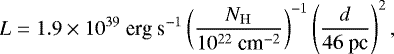
If we neglect flux dilution along the filament, we can apply the simple derivation given by Sunyaev & Churazov (1998) to infer the typical minimal brightness of the illuminating source. Because the cloud is not spherical here, we have to correct the formula for the apparent size of the filament seen from the illuminating source. Remembering that the cloud has to be tangent to the paraboloid of equal delays to be quickly illuminated, we can conclude that the apparent size of the filament seen from Sgr A⋆ is the same as its apparent size for the observer at infinity, because of the geometrical properties of the parabola. We therefore get the luminosity of the illuminating event:
 (2)
(2)
where d is the physical distance from Sgr A⋆ to the centre of the filament. Weassumed an E−2 power-law spectrum to estimate the luminosity over the 2 to 10 keV range. This value is consistent with values obtained for other clouds in the CMZ.
It is likely that the illuminating event is one of those visible in the Sgr A complex and discussed in Sect. 4.1 and in Clavel et al. (2013). The apparent connection with the G0.11–0.11 cloud, visible both at 6.4 keV and in CS molecule line maps, suggests that the signal in the latter cloud is now propagating in G0.24–0.17. Further monitoring of the filament will be necessary to see whether the time behaviour is similar. A rapid decay of the flux would suggest a shorter event than the one observed in G0.11–0.11.
6 Conclusions
We have performed a systematic analysis of Fe Kα line variations in the central 300 pc with XMM-Newton over a period spanning 12 yr from 2000 to 2012. In particular, two complete surveys of the region were performed in 2000–2001 and 2012 and allow a comparison of variations of the line flux. We find that, in the limit of the surveys’ sensitivity, most of the Fe Kα bright regions show significant variations between the two dates. This excludes sub-relativistic ion bombardment as the origin of the bright regions since their cooling time is significantly longer. We cannot exclude that cosmic rays play a significant role in some fainter, constant, diffuse 6.4 keV emission regions (as discussed, e.g. in Capelli et al. 2012). Yet, we note that Dogiel et al. (2013) have shown that such a scenario applied to the overall diffuse 6.4 keV emission in the CMZ would lead to ionization levels, as inferred from H molecule emission, much larger than observed.
The rapid variations of the 6.4 keV bright regions are also evidence that the reflection consists of relatively brief illumination episodes, lasting typically 10 yr or less. If a long duration steady illumination was significantly contributing to the illumination of the inner 300 pc, we should have observed regions of bright and stable Fe Kα emission. The conclusion of Clavel et al. (2013) that at least two distinct events, with typical durations of 2 and 10 yr, are required to explain the variations is confirmed. This is supported by the presence of variations on two distinct time scales observed in the Sgr A complex, by the rapid variations observed in the Sgr B complex and by the measurement of a displacement of the illumination in the Sgr C region. Whether more events are required is still an open question. In particular, we note that the emission from the more distant Sgr D complex could have a significantly larger delay and could be caused by a more ancient event.
Calculation of the exact date of the outbursts will require detailed spectral modelling of molecular clouds (Walls et al. 2016; Chuard et al. 2018). Other approaches based on the apparent velocity of reflected features would also allow one to date the illumination (Churazov et al. 2017b) assuming it is caused by a single flash. Further monitoring of the illuminated regions will be crucial to disentangle illumination and matter distribution effects. Long-term evolution of the reflection as well as X-ray polarimetric observations will also help constrain the location of the illuminating source (Churazov et al. 2017a).
Acknowledgements
The authors acknowledge the Centre National d’Études Spatiales (CNES) for financialsupport. G.P. acknowledges support via an EU Marie Curie Intra-European fellowship under contract no. FP-PEOPLE-2012-IEF-331095. This work has been partly supported by the LabEx UnivEarthS6 project “Impact of black holes on their environment”. Partial support through the COST action MP0905 Black Holes in a Violent Universe is acknowledged.
Appendix A: Regions
A.1: Regions excluded from analysis
To avoid pollution by bright point sources, we have excluded circular regions around a number of bright objects. Transients objects are removed only during periods when their emission is bright. The list of removed sources is given in Table A.1.
Exclusion regions corresponding to known bright transient and persistent sources in the CMZ.
Parameters of the regions of interest considered in this work.
A.2: 6.4 keV bright regions
Light curveshave been extracted in various regions to study variability of the 6.4 keV emission. A large fraction of these regions have been previously studied and the rest was found thanks to the systematic search for variability described above. The regions are ellipses and we give their parameters (centre coordinates, radii and rotation angle) in Table A.1. We note that the region G0.24–0.17 is a polygon in our analysis. For simplicity we give the parameters of an ellipse matching as closely as possible its morphology. Regions used to estimate the background level in different regions of the CMZ are also given.
References
- Amo-Baladrón, M. A., Martín-Pintado, J., Morris, M. R., Muno, M. P., & Rodríguez-Fernández, N. J. 2009, ApJ, 694, 943 [NASA ADS] [CrossRef] [Google Scholar]
- Barrière, N. M., Tomsick, J. A., Baganoff, F. K., et al. 2014, ApJ, 786, 46 [NASA ADS] [CrossRef] [Google Scholar]
- Bland-Hawthorn, J., Maloney, P. R., Sutherland, R. S., & Madsen, G. J. 2013, ApJ, 778, 58 [NASA ADS] [CrossRef] [Google Scholar]
- Boehle, A., Ghez, A. M., Schödel, R., et al. 2016, ApJ, 830, 17 [NASA ADS] [CrossRef] [Google Scholar]
- Capelli, R., Warwick, R. S., Porquet, D., Gillessen, S., & Predehl, P. 2011, A&A, 530, A38 [NASA ADS] [CrossRef] [EDP Sciences] [Google Scholar]
- Capelli, R., Warwick, R. S., Porquet, D., Gillessen, S., & Predehl, P. 2012, A&A, 545, A35 [NASA ADS] [CrossRef] [EDP Sciences] [Google Scholar]
- Chuard, D., Terrier, R., Goldwurm, A., et al. 2018, A&A, 610, A34 [NASA ADS] [CrossRef] [EDP Sciences] [Google Scholar]
- Churazov, E., Khabibullin, I., Ponti, G., & Sunyaev, R. 2017a, MNRAS, 468, 165 [NASA ADS] [CrossRef] [Google Scholar]
- Churazov, E., Khabibullin, I., Sunyaev, R., & Ponti, G. 2017b, MNRAS, 465, 45 [NASA ADS] [CrossRef] [Google Scholar]
- Clavel, M., Terrier, R., Goldwurm, A., et al. 2013, A&A, 558, A32 [NASA ADS] [CrossRef] [EDP Sciences] [Google Scholar]
- Clavel, M., Soldi, S., Terrier, R., et al. 2014, MNRAS, 443, L129 [NASA ADS] [CrossRef] [Google Scholar]
- Dogiel, V. A., Chernyshov, D. O., Tatischeff, V., Cheng, K.-S., & Terrier, R. 2013, ApJ, 771, L43 [Google Scholar]
- Fukuoka, R., Koyama, K., Ryu, S. G., & Tsuru, T. G. 2009, PASJ, 61, 593 [NASA ADS] [Google Scholar]
- Goldwurm, A., David, P., Foschini, L., et al. 2003, A&A, 411, L223 [NASA ADS] [CrossRef] [EDP Sciences] [Google Scholar]
- Guo, F., & Mathews, W. G. 2012, ApJ, 756, 181 [NASA ADS] [CrossRef] [Google Scholar]
- Handa, T., Sakano, M., Naito, S., Hiramatsu, M., & Tsuboi, M. 2006, ApJ, 636, 261 [NASA ADS] [CrossRef] [Google Scholar]
- Inui, T., Koyama, K., Matsumoto, H., & Tsuru, T. G. 2009, PASJ, 61, 241 [Google Scholar]
- Jones, P. A., Burton, M. G., Cunningham, M. R., Tothill, N. F. H., & Walsh, A. J. 2013, MNRAS, 433, 221 [NASA ADS] [CrossRef] [Google Scholar]
- Koyama, K., Maeda, Y., Sonobe, T., et al. 1996, PASJ, 48, 249 [NASA ADS] [CrossRef] [Google Scholar]
- Koyama, K., Inui, T., Hyodo, Y., et al. 2007, PASJ, 59, 221 [NASA ADS] [CrossRef] [Google Scholar]
- Krivonos, R. A., Tomsick, J. A., Bauer, F. E., et al. 2014, ApJ, 781, 107 [NASA ADS] [CrossRef] [Google Scholar]
- Miller, C. J., Genovese, C., Nichol, R. C., et al. 2001, AJ, 122, 3492 [NASA ADS] [CrossRef] [Google Scholar]
- Molinari, S., Bally, J., Noriega-Crespo, A., et al. 2011, ApJ, 735, L33 [NASA ADS] [CrossRef] [Google Scholar]
- Morris, M., & Serabyn, E. 1996, ARA&A, 34, 645 [NASA ADS] [CrossRef] [Google Scholar]
- Muno, M. P., Baganoff, F. K., Brandt, W. N., Park, S., & Morris, M. R. 2007, ApJ, 656, L69 [NASA ADS] [CrossRef] [Google Scholar]
- Murakami, H., Koyama, K., Sakano, M., Tsujimoto, M., & Maeda, Y. 2000, ApJ, 534, 283 [NASA ADS] [CrossRef] [Google Scholar]
- Murakami, H., Koyama, K., & Maeda, Y. 2001a, ApJ, 558, 687 [NASA ADS] [CrossRef] [Google Scholar]
- Murakami, H., Koyama, K., Tsujimoto, M., Maeda, Y., & Sakano, M. 2001b, ApJ, 550, 297 [NASA ADS] [CrossRef] [Google Scholar]
- Nakajima, H., Tsuru, T. G., Nobukawa, M., et al. 2009, PASJ, 61, 233 [NASA ADS] [Google Scholar]
- Nakashima, S., Nobukawa, M., Tsuru, T. G., Koyama, K., & Uchiyama, H. 2010, PASJ, 62, 971 [NASA ADS] [CrossRef] [Google Scholar]
- Nakashima, S., Nobukawa, M., Uchida, H., et al. 2013, ApJ, 773, 20 [NASA ADS] [CrossRef] [Google Scholar]
- Neilsen, J., Nowak, M. A., Gammie, C., et al. 2013, ApJ, 774, 42 [NASA ADS] [CrossRef] [Google Scholar]
- Nobukawa, M., Tsuru, T. G., Takikawa, Y., et al. 2008, PASJ, 60, S191 [NASA ADS] [CrossRef] [Google Scholar]
- Nobukawa, M., Ryu, S. G., Tsuru, T. G., & Koyama, K. 2011, ApJ, 739, L52 [NASA ADS] [CrossRef] [Google Scholar]
- Nowak, M. A., Neilsen, J., Markoff, S. B., et al. 2012, ApJ, 759, 95 [NASA ADS] [CrossRef] [Google Scholar]
- Ponti, G., Terrier, R., Goldwurm, A., Belanger, G., & Trap, G. 2010, ApJ, 714, 732 [NASA ADS] [CrossRef] [Google Scholar]
- Ponti, G., Morris, M. R., Terrier, R., & Goldwurm, A. 2013, in Cosmic Rays in Star-Forming Environments, eds. D. F. Torres, & O. Reimer, Astrophys. Space Sci. Proc., 34,331 [NASA ADS] [CrossRef] [Google Scholar]
- Ponti, G., Morris, M. R., Clavel, M., et al. 2014, in The Galactic Center: Feeding and Feedback in a Normal Galactic Nucleus, eds. L. O. Sjouwerman, C. C. Lang, & J. Ott, IAU Symp., 303, 333 [NASA ADS] [Google Scholar]
- Ponti, G., Bianchi, S., Muñoz-Darias, T., et al. 2015a, MNRAS, 446, 1536 [NASA ADS] [CrossRef] [Google Scholar]
- Ponti, G., De Marco, B., Morris, M. R., et al. 2015b, MNRAS, 454, 1525 [NASA ADS] [CrossRef] [Google Scholar]
- Ponti, G., Morris, M. R., Terrier, R., et al. 2015c, MNRAS, 453, 172 [NASA ADS] [CrossRef] [Google Scholar]
- Porquet, D., Grosso, N., Predehl, P., et al. 2008, A&A, 488, 549 [NASA ADS] [CrossRef] [EDP Sciences] [Google Scholar]
- Protheroe, R. J., Ott, J., Ekers, R. D., Jones, D. I., & Crocker, R. M. 2008, MNRAS, 390, 683 [NASA ADS] [Google Scholar]
- Ryu, S. G. 2013, Ph.D. thesis, Kyoto University, Japan [Google Scholar]
- Ryu, S. G., Nobukawa, M., Nakashima, S., et al. 2013, PASJ, 65, 33 [NASA ADS] [CrossRef] [Google Scholar]
- Sakano, M., Warwick, R. S., & Decourchelle, A. 2006, J. Phys. Conf. Ser., 54, 133 [NASA ADS] [CrossRef] [Google Scholar]
- Sawada, M., Tsujimoto, M., Koyama, K., et al. 2009, PASJ, 61, S209 [NASA ADS] [Google Scholar]
- Sidoli, L., Mereghetti, S., Treves, A., et al. 2001, A&A, 372, 651 [NASA ADS] [CrossRef] [EDP Sciences] [Google Scholar]
- Sidoli, L., Mereghetti, S., Favata, F., Oosterbroek, T., & Parmar, A. N. 2006, A&A, 456, 287 [NASA ADS] [CrossRef] [EDP Sciences] [Google Scholar]
- Snowden, S. L., Mushotzky, R. F., Kuntz, K. D., & Davis, D. S. 2008, A&A, 478, 615 [NASA ADS] [CrossRef] [EDP Sciences] [Google Scholar]
- Su, M., Slatyer, T. R., & Finkbeiner, D. P. 2010, ApJ, 724, 1044 [NASA ADS] [CrossRef] [Google Scholar]
- Sunyaev, R., & Churazov, E. 1998, MNRAS, 297, 1279 [NASA ADS] [CrossRef] [Google Scholar]
- Sunyaev, R. A., Markevitch, M., & Pavlinsky, M. 1993, ApJ, 407, 606 [NASA ADS] [CrossRef] [Google Scholar]
- Tatischeff, V., Decourchelle, A., & Maurin, G. 2012, A&A, 546, A88 [Google Scholar]
- Terrier, R., Ponti, G., Bélanger, G., et al. 2010, ApJ, 719, 143 [NASA ADS] [CrossRef] [Google Scholar]
- Tsuboi, M., Tadaki, K.-I., Miyazaki, A., & Handa, T. 2011, PASJ, 63, 763 [NASA ADS] [CrossRef] [Google Scholar]
- Walls, M., Chernyakova, M., Terrier, R., & Goldwurm, A. 2016, MNRAS, 463, 2893 [NASA ADS] [CrossRef] [Google Scholar]
- Wang, Q. D., Nowak, M. A., Markoff, S. B., et al. 2013, Science, 341, 981 [NASA ADS] [CrossRef] [Google Scholar]
- Yusef-Zadeh, F., Law, C., & Wardle, M. 2002, ApJ, 568, L121 [NASA ADS] [CrossRef] [Google Scholar]
- Zhang, S., Hailey, C. J., Mori, K., et al. 2015, ApJ, 815, 132 [NASA ADS] [CrossRef] [Google Scholar]
- Zubovas, K., King, A. R., & Nayakshin, S. 2011, MNRAS, 415, L21 [NASA ADS] [CrossRef] [Google Scholar]
http://xmm2.esac.esa.int/external/xmm_sw_cal/calib/epic_files.shtml. It is position dependent, especially for the EPIC/pn, due to changing energy resolution when moving from the optical axis to the detector edges. Maps of the position-dependent correction factor were computed for each instrument based on its redistribution matrix. For each observation and instrument, the corrected net line flux is obtained by dividing the net counts maps by the corresponding efficiency map reprojected according to the astrometry.
There are no data from 2010 in our data set.
We considered that variability can be detected in pixels whose light curves have (1) at least 2 degrees of freedom for the constant fit and at least 3 for the linear fit; (2) at least one data point detected at more than 3σ; (3) a minimum detectable absolute slope for a linear fit ≤ 0.7 × 10⁻⁷ ph cm−2 s−1 arcmin−2 yr−1, where the minimum slope is the smallest between that determined by the largest error bars of the data points in the light curve and that provided by the error bars of the two most distant points (in time) in the light curve.
We note that we have little exposure farther out and that we might miss emission from a fraction of the elongated matter structure. We note also that the morphology of the emission observed by Suzaku is very similar to that in our 2012 image.
The “Sgr D core” region we consider here is only partly included in the larger region chosen for the Suzaku analysis (Ryu 2013), so this additional 6.4 keV measurement in 2007 could not be used in our variability analysis.
This region has a box shape, not an elliptical one.
All Tables
Exclusion regions corresponding to known bright transient and persistent sources in the CMZ.
All Figures
|
Fig. 1 Time exposure maps for the 7 epochs in which the XMM-Newton data have been grouped (in units of seconds, with 2.5″ pixel size, and in Galactic coordinates) after applying the exposure time cuts discussed in Sect. 2.1. The darker circular regions correspond to the point sources that have been excluded (see the list in Table A.1). The MOS1 and MOS2 exposures have been rescaled to take into account the different MOS and PN effective areas in order to create the PN-equivalent exposure mosaics shown here. |
| In the text | |
|
Fig. 2 Comparison of the Fe Kα fluxes extracted from the mosaic images with those obtained from the spectral fitting for the four test regions within 12′ of Sgr A⋆ visible in the inset. The data have been grouped into eight periods as described in the text (with the 2012 data split between the March and autumn observations). The dashed line indicates where regions with the same fluxes from imaging andspectral analysis should lie and the dotted lines represent the 10% dispersion around it. |
| In the text | |
|
Fig. 3 Background- and continuum-subtracted intensity maps of the inner GC region measured by XMM-Newton at 6.4 keV in 2000–2001 (top) and 2012 (bottom). The maps are in units of ph cm −2 s −1 pixel−1, with 2.5″ pixel size, and smoothed using a Gaussian kernel of 5 pixels radius. The dotted square regions are discussed in more detail in Sect. 4. |
| In the text | |
|
Fig. 4 Histogram of the significance of variations of Fe Kα line emission in 1′ pixels between the 2000–2001 and 2012 surveys. Nearly all pixels with a brightness larger than 3 × 10⁻⁶ ph cm−2 s−1 arcmin−2 are found tovary. |
| In the text | |
|
Fig. 5 Maps resulting from the variability study of 7 periods from 2000 to 2012, using a 1′ pixel size. Top: significance of rejection for a fit with a constant-intensity model applied to each bin light curve, and after performing aχ2 smoothing (see text for details). Centre: same as top panel but applying a linear fit. Bottom: slope of the linear fit for the pixels for which variability can be detected and with non-zero significance shown in the top panel. |
| In the text | |
|
Fig. 7 Fe Kα light curve of the illuminated clouds in the Sgr A complex (regions indicated in Fig. 6). The blue band shows the level of background line emission estimated in a large region below Sgr A⋆. All errors shown on the light curves are 1σ errors (68% confidence level). |
| In the text | |
|
Fig. 6 Fe Kα flux images of the Sgr A complex in the period 2000–2012. The dotted lines mark the regions discussed in the text and whose light curves are extracted. The bottom right panel shows the same regions, as grey ellipses, compared to the various structures of the molecular complexes traced by CS shown as solid lines (blue −20–10 km s−1, red 10–40 km s−1 and green 40–70 km s−1). Short timescale (≲2 yr) variations are mostly visible in structures in the last velocity range. |
| In the text | |
|
Fig. 8 Fe Kα images of the Sgr B complex. The right panel shows the total gas column density measured by Herschel (Molinari et al. 2011). |
| In the text | |
|
Fig. 9 Fe Kα light curves of the Sgr B complex integrated over the regions indicated in Fig. 8. All errors shown on the light curves are 1σ errors (68% confidence level). |
| In the text | |
|
Fig. 10 Fe Kα maps of the Sgr C complex for three periods of XMM-Newton observations (first three panels from the left) and Mopra HCN map integrated over the − 80 to − 60 km s−1 velocity band for the same region (right panel). The yellow, green, and cyan dots give the position of the centroid of the emission in the C1 region in 2000−2001, 2006−2007 and 2012, respectively. A displacement of 1.6′ of the emission in a direction similar to that of the molecular feature is visible. The Fe Kα maps are in units of ph cm−2 s−1 pixel−1, with 2.5″ pixel size, and smoothed using a Gaussian kernel of 8 pixels radius. The solid line region labelled Sgr C includes the bulk of the Fe Kα bright clumps, while the smaller regions reported by other papers plus the C4 clump newly labelled here are shown in dotted lines. |
| In the text | |
|
Fig. 11 Fe Kα light curves of the Sgr C complex (circles) integrated over the regions indicated in Fig. 10. The blue band indicates the level of background emission measured in a large region defined in Table A.2. All errors shown on the light curves are 1σ errors (68% confidence level). |
| In the text | |
|
Fig. 12 Left: Fe Kα maps centred at the position of the M359.23–0.04 structure during the 2000–2001 and 2012 XMM-Newton observations. The maps are in units of ph cm−2 s−1 pixel−1, with 2.5″ pixel size, and smoothed using a Gaussian kernel of 15 pixels in radius. Right: CS(1–0) map integrated in the −140 to −120 km s −1 velocity band. |
| In the text | |
|
Fig. 13 Left: Fe Kα map centred at the position of Sgr D during the 2012 XMM-Newton observations. The map is in units of ph cm −2 s−1 pixel−1, with 2.5″ pixel size, and smoothed using a Gaussian kernel of 15 pixels radius. The region labelled Sgr D includes the bulk of the Fe Kα emission in the complex. Middle: CS map integrated in the velocity range 50 to 70 km s−1 showing the molecular counterpart of the 6.4 keV emission. Right: Fe Kα light curve of the Sgr D complex integrating over the region indicated on the maps. The blue band indicates the level of background emission. All errors shown on the light curves are 1σ errors (68% confidence level). |
| In the text | |
|
Fig. 14 Left images: Fe Kα maps centred at the position of the G0.24–0.17 filament during the 2000–2001 and 2012 XMM-Newton observations. The maps are in units of ph cm−2 s−1 pixel−1, with 2.5″ pixel size, and smoothed using a Gaussian kernel of 8 pixels in radius. Centre: Mopra CS(1–0) map integrated over the 27–35 km s−1 velocity band. Right: Fe Kα light curve of the G0.24–0.17 filament. The blue band indicates the level of background emission measured in a circular region south of Sgr A⋆. All errors shown on the light curves are 1σ errors (68% confidence level). |
| In the text | |
Current usage metrics show cumulative count of Article Views (full-text article views including HTML views, PDF and ePub downloads, according to the available data) and Abstracts Views on Vision4Press platform.
Data correspond to usage on the plateform after 2015. The current usage metrics is available 48-96 hours after online publication and is updated daily on week days.
Initial download of the metrics may take a while.