| Issue |
A&A
Volume 612, April 2018
|
|
|---|---|---|
| Article Number | A36 | |
| Number of page(s) | 15 | |
| Section | Interstellar and circumstellar matter | |
| DOI | https://doi.org/10.1051/0004-6361/201730561 | |
| Published online | 17 April 2018 | |
Radio and infrared study of southern H II regions G346.056−0.021 and G346.077−0.056★
1
Indian Institute of Space Science and Technology,
Trivandrum
695547, India
e-mail: swagat.12@iist.ac.in
2
Korea Astronomy and Space Science Institute 776,
Daedeokdae-ro, Yuseong-gu,
Daejeon
305-348, Republic of Korea
3
East Asian Observatory,
660 N. A’ohoku Place,
Hilo, HI
96720, USA
4
National Centre For Radio Astrophysics,
Pune
411007,
India
Received:
4
February
2017
Accepted:
4
October
2017
Aim. We present a multiwavelength study of two southern Galactic H II regions G346.056−0.021 and G346.077−0.056 which are located at a distance of 10.9 kpc. The distribution of ionized gas, cold and warm dust, and the stellar population associated with the two H II regions are studied in detail using measurements at near-infrared, mid-infrared, far-infrared, submillimeter and radio wavelengths.
Methods. The radio continuum maps at 1280 and 610 MHz were obtained using the Giant Metrewave Radio Telescope to probe the ionized gas. The dust temperature, column density, and dust emissivity maps were generated using modified blackbody fits in the far-infrared wavelength range 160–500 μm. Various near- and mid-infrared color and magnitude criteria were adopted to identify candidate ionizing star(s) and the population of young stellar objects in the associated field.
Results. The radio maps reveal the presence of diffuse ionized emission displaying distinct cometary morphologies. The 1280 MHz flux densities translate to zero age main sequence spectral types in the range O7.5V–O7V and O8.5V–O8V for the ionizing stars of G346.056−0.021 and G346.077−0.056, respectively. A few promising candidate ionizing star(s) are identified using near-infrared photometric data. The column density map shows the presence of a large, dense dust clump enveloping G346.077−0.056. The dust temperature map shows peaks towards the two H II regions. The submillimeter image shows the presence of two additional clumps, one being associated with G346.056−0.021. The masses of the clumps are estimated to range between ~1400 and 15250 M⊙. Based on simple analytic calculations and the correlation seen between the ionized gas distribution and the local density structure, the observed cometary morphology in the radio maps is better explained invoking the champagne-flow model.
Key words: infrared: ISM / radio continuum: ISM / HII regions / ISM: individual objects: G346.056–0.021 / ISM: individual objects: G346.077–0.056
GMRT data (FITS format) are only available at the CDS via anonymous ftp to cdsarc.u-strasbg.fr (130.79.128.5) or via http://cdsarc.u-strasbg.fr/viz-bin/qcat?J/A+A/612/A36
© ESO 2018
1 Introduction
Massive O and B star formation is accompanied by enormous Lyman continuum emission. The outpouring of UV photons ionize the surrounding interstellar medium (ISM) forming H II regions and thus revealing the location of ongoing high-mass star formation through radio free-free emission. In the evolutionary sequence, it starts with the deeply embedded, hypercompact H II regions which eventually expand forming the ultra-compact (UCH II ), compact, and extended or classical H II regions. The earliest evolutionary phase is closely linked to the formation process where the newly born massive star is still in the accretion phase. The classical H II regions on the other hand are mostly associated with more evolved objects. Apart from being bright in the radio, the high luminosity of the massive stars also makes the H II regions bright in the infrared (IR). The UV and optical radiation from the star is absorbed by the dust and is re-emitted in the IR. The radio and the thermal IR being least affected by extinction, studies in these wavelength regimes allow us to probe deep into the star forming clouds to unravel the processes associated with high-mass star formation and the cooler dust environment. Complimentary near-infrared (NIR) studies further provide the census of the associated young stellar population. Excellent reviews on the nature and physical properties of H II regions can be found in Hoare et al. (2007), Wood & Churchwell (1989), Churchwell (2002), Garay & Lizano (1999).
In this paper, we study two southern H II regions from IR through radio wavelengths. These are G346.056−0.021 and G346.077−0.056. IRAS 17043−4027, with IRAS colors consistent with UCH II regions (Bronfman et al. 1996), is associated with G346.077−0.056. From the 13CO observationsof candidate massive young stellar objects (YSOs) in the southern Galactic plane, Urquhart et al. (2007b) give the kinematic distance estimate of 5.7 kpc (near) and 10.8 kpc (far) for G346.056−0.021 and 5.8 kpc (near) and 10.7 kpc (far) for G346.077−0.056. In a later paper (Urquhart et al. 2014), they resolve the kinematic distance ambiguity by using H I self-absorption analysis and place both the sources at the far-distance of 10.9 kpc. We adopt this distance in our study. As part of the Green Bank Telescope (GBT) H II Region Discovery Survey, hydrogen radio recombination line (RRL) emission was detected towards G346.056−0.021 and G346.077−0.056 (Anderson et al. 2011) and helium and carbon RRLs were observed towards G346.056−0.021 (Wenger et al. 2013). From their 1400 MHz Galactic plane survey, Zoonematkermani et al. (1990) listed G346.056−0.021 and G346.077−0.056 as small diameter radio sources with sizes of 18′′.8 and 9′′, respectively. Apart from this, G346.077−0.056 was observed at 4800 and 8640 MHz by Urquhart et al. (2007a) as part of the Red MSX Sources (RMS) survey to obtain radio observations of candidate massive YSOs. Other than the 13CO survey mentioned above, a few other molecular line studies have been conducted toward G346.077−0.056 (Bronfman et al. 1996; Hoq et al. 2013; Yu et al. 2015). G346.077−0.056 has been part of a 6.7 GHz methanol maser detection survey which yielded negative results (van der Walt et al. 1995). A similar result was also obtained from the recent 6.7 GHz methanol maser survey (Caswell et al. 2010). Further, a sparsely populated embedded cluster, VVV CL094, is reported to be associated with G346.077−0.056 (Borissova et al. 2011; Morales et al. 2013). As is evident from the literature survey, there have been no dedicated studies of either of these two H II regions.
Figure 1 displays a color-composite image of the associated region showing the location and the dust environment. The 8 μm emission is relatively localized towards the center of G346.077−0.056 as compared to G346.056−0.021 where it displays an extended bubble-type morphology towards the south-west. Probing the warm dust component, 24 μm emission is seen predominantly towards G346.056−0.021 and the central portion of G346.077−0.056. The 870 μm component which traces the cold dust environment is seen as a prominent, large clump enveloping G346.077−0.056 with a distinct filamentary structure towards the west connecting to G346.056−0.021.
Presenting a multiwavelength study of the complex associated with these two H II regions, we have organized the paper in the following way. Section 2 describes the radio continuum observation and the associated data reduction procedure. In this section, we have also discussed the various archival data used in this study. Study of the ionized and the dust component and the associated stellar population is presented in Sect. 3. Possible mechanisms responsible for the morphology of the ionized emission for both H II regions are explored in Sect. 4. The summary of the results obtained is compiled in Sect. 5.
2 Observation and archival data sets
2.1 Radio continuum observations
To probe the ionized emission associated with the H II regions, radio continuum mapping was carried out at 610 and 1280 MHz using the Giant Metrewave Radio Telescope (GMRT), Pune India. GMRT contains 30 dishes of 45 m diameter, each arranged in a hybrid “Y” shaped configuration. This ensures a wide UV coverage. The central square of GMRT has 12 antennae randomly arranged within a compact area of 1 × 1 km2. The remaining 18 antennae are placed in the arms of the “Y” with each arm comprising six antennae. With the possible baselines ranging between ~ 100 m and ~ 25 km, GMRT enables us to probe the ionized emission at various resolutions and spatial scales. Swarup et al. (1991) provides detail information regarding GMRT and its configuration.
The continuum observations were carried out at 610 and 1280 MHz with a bandwidth of 32 MHz. This was done in the spectral line mode to minimize the effects of bandwidth smearing and narrowband RFI. The on-source integration time is ~ 4 h. The radio sources 3C48 and 3C286 were used as primary flux calibrators and 1626−298 was used as a phase calibrator. These provide the amplitude and phase gains for flux and phase calibration of the measured visibilities, respectively. Data reduction was carried out using Astronomical Image Processing System (AIPS). The tasks UVPLT, VPLOT and TVFLG were used to check the data carefully and bad data (dead antenna, dead baseline, spikes, RFI, etc.) were edited out using the tasks TVFLG and UVFLG. To keep the bandwidth smearing effect negligible the calibrateddata were averaged in frequency. We adopt the wide-field imaging technique to account for the w-term effect. Several iterations of “phase-only” self calibration were done to minimize amplitude and phase errors and obtain better rms noise in the maps. Primary beam correction was applied with the task PBCOR.
While observing towards the Galactic plane, the contribution from the Galactic diffuse emission is appreciable and leads to the rise in system temperature. The flux calibration is based on the sources which are off the Galactic plane. Hence, it becomes essential to rescale the generated maps. G346.056−0.021 and G346.077−0.056 are located north-east of the bubble S10 which is studied in detail in Ranjan Das et al. (2016). Both these H II regions were observed as part of the same field with S10 being at the phase center. Thus we use the same scaling factors of 1.2 (1280 MHz) and 1.7 (610 MHz) derived in Ranjan Das et al. (2016).
2.2 Archival data sets
2.2.1 Near-infrared data from VVV and 2MASS
NIR (JHK/K_s) photometric data for point sources around our region of interest are obtained from the VISTA Variables in Via Lactea (VVV; Minniti et al. 2010) and Two Micron All Sky Survey Point Source Catalog (2MASSPSC; Skrutskie et al. 2006). The VVV and 2MASS images have resolutions of ~0.8′′and 5′′, respectively. Good quality photometric data are retrieved from these catalogs and used to study the nature of the stellar population associated with the two H II regions.
2.2.2 Mid-infrared data from Spitzer
Mid-infrared (MIR) data enclosing the two H II regions have been obtained from the archive of Spitzer Space Telescope. The Infra-Red Array Camera (IRAC) and Multiband Imaging Photometer (MIPS) are the two onboard instruments. Simultaneous images at 3.6, 4.5, 5.8, 8.0 μm are obtained by IRAC with angular resolutions <2′′ (Fazio et al. 2004). The Level-2 Post-Basic Calibrated Data (PBCD) images from the Galactic Legacy Infrared Mid-Plane Survey Extraordinaire (GLIMPSE; Benjamin et al. 2003) and photometric data from the “highly reliable” GLIMPSE I Spring’07 catalog are used in this paper. These data are used to study the population of young stellar objects (YSOs) and warm dust associated with the regions.
2.2.3 Far-infrared data from Herschel
Far-infrared (FIR) maps for our regions in the wavelength range 70–500 μm were retrieved from the Herschel Space Observatory archives. These regions were observed as part of the Herschel Infrared Galactic Plane Survey (HI-GAL; Molinari et al. 2010). We used the images obtained with the Photodetector Array Camera and Spectrometer (PACS; Poglitsch et al. 2010) and Spectral and Photometric Imaging Receiver (SPIRE; Griffin et al. 2010). We used Level-2 PACS images at 70 and 160 μm and Level-3 SPIRE images at 250, 350 and 500 μm from the archive for our study. The images used have resolutions of 5′′.9, 11′′.6, 18′′.5, 25′′.3 and 36′′.9 and pixel sizes of 3′′.2, 3′′.2, 6′′, 10′′and 14′′at 70, 160, 250, 350, and 500 μm, respectively.The Herschel Interactive Processing Environment (HIPE)1 is used for processing the images. We used the FIR data to study the physical properties of cold dust emission associated with the regions.
2.2.4 870 μm data from ATLASGAL
The 870 μm image used in this study has been obtained from the archivesof the Apex Telescope under the Apex Telescope Large Area Survey of the Galaxy (ATLASGAL)2 which used the LABOCA bolometer array (Schuller et al. 2009). The resolution of ATLASGAL image is 18.2′′. This data is used to study the properties of cold dust clumps associated with these H II regions.
3 Results and discussion
3.1 Emission from ionized gas
The radio emission associated with the two H II regions mapped at 610 and 1280 MHz is shown in Fig. 2. These maps are generated by setting the “robustness” parameter to −5 (on a scale where +5 represents pure natural weighting and −5 is for pure uniform weighting of the baselines) while running the task IMAGR and considering the entire uv coverage. However, for probing the larger spatial scales of the extended diffuse, ionized emission in these regions we also generate continuum maps by setting the “robustness” parameter to +1 and weigh down the long baselines using the task UVTAPER. These lower resolution maps are shown in Fig. 3. The details of observation and the generated maps are listed in Table 1. The positional offsets of the peaks in these maps are within ~2′′.
As seen from the figures, the ionized emission associated with the H II region G346.056−0.021 displays a distinct cometary morphology at both 610 and 1280 MHz with a steep intensity gradient towards the east. A faint, broad and diffuse tail is seen towards the west-south-west. The observed morphology suggests that this H II region is density bounded towards the south-west and ionization bounded towards the north-east. The emission from G346.077−0.056 is also seen to be cometary in nature with the signature being more pronounced at 1280 MHz. The higher-resolution maps more closely corroborate the above picture. The higher-resolution 1280 MHz map displays an interesting morphology where a compact, cometary structure is seen towards the west of G346.077−0.056. This could possibly be another H II region with its cometary head facing that of G346.077−0.056. However, we cannot rule out the other possibility of an externally ionized clump arising due to density inhomogeneities. An extended low-intensity (at 3σ level) detached component is also seen at 1280 MHz in Fig. 3. It is difficult to ascertain the physical association of this feature with G346.077−0.056. Using the Australia Telescope Compact Array, Urquhart et al. (2007a) observed the two regions at 3.6 cm (8640 MHz) and 6.0 cm (4800 MHz) with a spatial resolution of ~1–2′′and sensitivity ~0.3 mJy. Radio emission is detected at both frequencies for G346.077−0.056 with the peak positions in good agreement (within 2.5′′) with the GMRT maps. They classified this H II region as one displaying a cometary morphology which is consonant with the GMRT maps. However, G346.056−0.021 is not listed under the RMS sources having associated radio emission. Table 2 allows a comparison of GMRT results with that of Urquhart et al. (2007a) and Zoonematkermani et al. (1990). The integrated flux densities derived from the GMRT 1280 MHz map is larger than that from the 1400 MHz VLA observations obtained by Zoonematkermani et al. (1990). This is understandable considering the fact that the integration time for their observation was only 120 s and hence not expected to be sensitive to the extended, faint diffuse emission. Similarly, the high-resolution ATCA maps would have also resolved out a good fraction of the diffuse emission.
For deriving the physical parameters of the two H II regions, we use the lower-resolution GMRT maps which sample most of the associated ionized emission. For this we first convolve the 1280 MHz map to the resolution of the 610 MHz map. From the peak flux densities at 610 and 1280 MHz, we estimate the radio spectral index α (Fν ∝ ν α) to be − 0.1 ± 0.06 and 0.01 ± 0.004 for G346.056−0.021 and G346.077−0.056, respectively. Taking the integrated flux densities, we estimate spectral index values of − 0.3 ± 0.06 and − 0.4 ± 0.06 for G346.056−0.021 and G346.077−0.056, respectively.Here, we have sampled the same region defined by the 3σ contour of the 610 MHz map. The spectral index values obtained from the peak flux densities are consistent with optically thin free-free emission. However, the values obtained from the integrated flux densities are indicative of non-thermalemission (Rosero et al. 2016; Kobulnicky & Johnson 1999; Rodriguez et al. 1993). Thus a scenario of co-existing free-free and non-thermal emission can be visualized for the H II regions as has been addressed by several authors (Russeil et al. 2016; Veena et al. 2016; Nandakumar et al. 2016; Mücke et al. 2002; Das et al. 2017). The above interpretation should be taken with caution because GMRT is not a scaled array between the observed frequencies and the observed visibilities span different uv ranges. This implies that the generated maps at 610 and 1280 MHz are sensitive to different spatial scales thus rendering the estimated spectral indices uncertain.
Following the method discussed in Quireza et al. (2006), Anderson et al. (2015), Luisi et al. (2016), we derive the electron temperature, Te , towards both these regions. This formulation assumes local thermodynamic equilibrium for the RRL lines, and is given by the following expression
![\begin{align*}&T_{e}[{\textrm{K}}] = \left \{ 7103.3 \left (\frac{\nu}{\textrm{GHz}}\right ){}^{1.1} \left (\frac{T_C}{T_L(\textrm{H}^+)}\right ) \left( \frac{{\mathrm{\Delta}} V(\textrm{H}^+)}{{\textrm{km\ s}^{-1}}} \right )^{-1} \right. \nonumber\\ &\qquad\quad \ \ \left. \times \left( 1+ \frac{{\textrm{n}({}^4\textrm{He}^+)}}{\textrm{n}(\textrm{H}^+)} \right )^{-1} \right \}^{0.87}, \end{align*}](/articles/aa/full_html/2018/04/aa30561-17/aa30561-17-eq1.png) (1)
(1)
where, ν is the observing frequency for the RRL lines, TC is the peak continuum antenna temperature, TL is the peak antenna temperature for hydrogen RRL line, ΔV (H+) is the full width at half maximum (FWHM) line width for the RRL line and  is the helium ionic abundance ratio. The hydrogen RRL line parameters for both the H II regions are taken from Anderson et al. (2011). The helium ionic abundance ratio has been derived from the hydrogen and helium RRL line properties and using the following equation (Quireza et al. 2006; Wenger et al. 2013)
 (2)
(2)
where TL is the peak line intensity and ΔV is the FWHM line width. We have derived the value of y+ to be 0.11 for the H II region G346.056−0.021 using the hydrogen and helium RRL line parameters from Wenger et al. (2013). For G346.077−0.056, no helium RRL observation is available, hence we use an average valueof y+ = 0.07 estimated from a sample of H II regions (Wenger et al. 2013). From the above expressions and observed parameters, we estimate the electron temperature to be 5500 K and 8900 K for the H II regions G346.056−0.021 and G346.077−0.056, respectively. These values fall within the range of ~5000 to ~10 000 K seen for Galactic H II regions (Quireza et al. 2006).
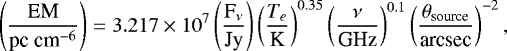
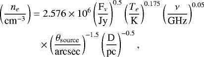
In order to derive the other physical properties of the ionized emission associated with the two H II regions, we adopted the expressions from Schmiedeke et al. (2016). Lucid explanations coupled with rigorous derivations of physical properties of H II regions can be found in the original papers of Mezger & Henderson (1967), Rubin (1968), Schraml & Mezger (1969), Panagia (1973). The H II regions are considered as Strömgren’s spheres which are fully ionized spherical regions of uniform electron density. Assuming the radio emission at 1280 MHz to be optically thin and emanating from a homogeneous, isothermal medium, the electron density, ne, the emission measure, EM, and the number of Lyman-continuum photons per second, NLy, are estimated using the following equations (Schmiedeke et al. 2016)
 (3)
(3)
 (4)
(4)
 (5)
(5)
where, Fν is the integrated flux density of ionized region, Te is the electron temperature, ν is the frequency, θsource is the angular diameter of the H II region, and D is the distance to these regions. Theangular extents of the ionized emission associated with G346.056−0.021 and G346.077−0.056 are estimated from the 1280 MHz map to be 61′′× 49′′and 34′′× 32′′, respectively. These values are the FWHMx ×FWHMy obtained using the 2D Clumpfind algorithm (Williams et al. 1994) for a 3σ threshold level. Applying beam corrections, we derive the deconvolved sizes to be 33′′× 38′′and 17′′× 19′′for G346.056−0.021 and G346.077−0.056, respectively. For θsource, we have taken the geometric mean of the deconvolved FWHM. The physical parameters thus derived are listed in Table 3.
If single zero age main sequence (ZAMS) stars are responsible for the ionization of the H II regions, then using Table I of Martins et al. (2005), the estimated Lyman continuum flux translates tospectral types O7.5V – O7V and O8.5V – O8V for G346.056−0.021 and G346.077−0.056, respectively.Similar spectral types are obtained if we use the results of Davies et al. (2011) and Mottram et al. (2011). If we consider the compact, cometary H IIregion seen in the higher-resolution 1280 MHz map to be internally ionized, then the integrated flux density implies a massive star of spectral type B0.5 – B0. The spectral type estimate for the ionizing star of G346.077−0.056 remains the same if we subtract out the flux density of this component. Taking the bolometric luminosities from the RMS survey paper by Lumsden et al. (2013) and comparing the same with the tables of Mottram et al. (2011), we obtain consistent spectral type estimates of O8 – O7.5 for both the H II regions. As mentioned earlier, this estimate is with the assumption of optically thin emission and hence servesas a lower limit as the emission could be optically thick at 1280 MHz. Several studies have shown that dust absorption of Lyman continuum photons can be very high (Inoue et al. 2001; Arthur et al. 2004; Paron et al. 2011). With limited knowledge of the dust properties, we have not accounted for the dust absorption in the above estimates. The Lyman continuum fluxes suggest massive stars of masses ~ 25 and ~ 20 M⊙ responsible for the ionized emission of G346.056−0.021 and G346.077−0.056, respectively (Davies et al. 2011).
We use a simple model discussed in Spitzer (1978), Dyson & Williams (1980) to estimate the dynamical ages of the two H IIregions. If an H II region evolves in a homogeneous medium then its dynamical age can be estimated from the following expressions
![\begin{align*} & R_{\textrm{st}} = \left[\frac{3\it N_{\textrm{Ly}}}{4\ \pi\ n_{H,0}^{2}\ \alpha_{B}} \right]^{1/3},\\ & t_{\textrm{dyn}} = \frac{4}{7}\ \frac{R_{\textrm{st}}}{C_{\textrm{Hii}}} \left[ \left(\frac{R_{\textrm{if}}}{R_{\textrm{st}}}\right)^{7/4}\ -1\right],\end{align*}](/articles/aa/full_html/2018/04/aa30561-17/aa30561-17-eq7.png) (6) (7)
(6) (7)
where, Rst is the Strömgren radius, NLy is the Lyman continuum photons coming from the ionizing source,nH,0 is the particle density of the neutral gas, and αB is the coefficient of radiative recombination and is taken to be 2.6 × 10⁻¹³ 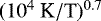 cm3 s−1 from Kwan (1997). In the second expression, tdyn is the dynamical age, CHii is the isothermal sound speed of ionized gas (assumed to be 10 km s−1), and Rif is the radius of the H II region. For Rif, we use the deconvolved sizes of 17′′(0.9 pc) and 9′′(0.5 pc) for G346.056−0.021 and G346.077−0.056, respectively. nH,0 is estimated from the column density map (refer to Sect. 3.3) and is found to be 6.2 × 104cm−3 and 4.8 × 104 cm−3 for G346.056−0.021 and G346.077−0.056, respectively. For G346.077−0.056, the estimated values of nH,0 is higher than that obtained by Yu et al. (2015) by a factor of approximately 6. Using these values in the above equations, we estimate the dynamical ages for G346.056−0.021 and G346.077−0.056 to be 0.5 and 0.2 Myr, respectively. The derived age should however be treated with caution since the assumption of expansion in a homogeneous medium is not a realistic one.
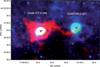 |
Fig. 1 Color composite image of the region associated with G346.056−0.021 and G346.077−0.056 using IRAC 8.0 μm band (see Sect. 2.2.2; blue), MIPS 24 μm (MIPSGAL Survey; Carey et al. 2009; green), and ATLASGAL 870 μm (see Sect. 2.2.4; red). Positions of the H II regions as listed in Anderson et al. (2011) are shown with the “×” symbols. The “+” symbol shows the position of IRAS 17043−4027. It should be noted here that a few pixels toward the central part of the 24 μm emission associated with G346.077−0.056 are saturated. |
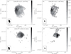 |
Fig. 2 Ionized emission associated with the H IIregions – panels a and b: 610 and 1280 MHz maps for the region associated with G346.056−0.021; panels c and d: 610 and 1280 MHz emission for the region around G346.077−0.056. The contourlevels are 3, 5, 10, 15, 20, 25, 30, and 35 times σ, where σ is equal to 0.3 mJy beam−1 and 0.2 mJybeam−1 at 610 MHz and 1280 MHz, respectively. Beam in each band is shown as filled ellipse. These maps are generated by setting the “robustness parameter” to −5 and withoutany uv tapering. |
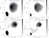 |
Fig. 3 Sameas in Fig. 2, but for maps generated with “robustness parameter” +1 and appropriate uv tapering to weigh down long baselines. The contour levels are 3, 5, 7, 11, 15, 20, 25, 30, 40, and 55 times σ where σ is 2.1 mJy beam−1 and 0.5 mJybeam−1 at 610 MHz and 1280 MHz, respectively. Beam in each band is shown as filled ellipse. |
Details of the radio interferometric continuum observations and generated maps.
GMRT, ATCA (Urquhart et al. 2007a), and 1.4 GHz (Zoonematkermani et al. 1990) results.
Derived physical parameters of H II regions.
3.2 Associated stellar population
Figure 4 shows the NIR view of the region associated with the two H II regions. The region is seen to be densely populated. The zoom of the region associated with G346.077−0.056 shows the presence of faint K-band nebulosity harboring the IR cluster VVVCL094 (Borissova et al. 2011). These authors have estimated the cluster radius to be 20′′. After a statistical decontamination of field star population, they propose 20 probable members for this cluster. As part of another statistical study of clusters in the inner Galaxy, Morales et al. (2013) classified VVVCL094 as an embedded cluster whose estimated center coincides with the ATLASGAL peak. Given the correlation of the cluster with the probed ionized region, it is likely that the most massive members of it are responsible for the detected H II region.
Using the NIR data from the VVV and 2MASS surveys, we attempt to identify candidate ionizing star(s) responsible for the H II regions and study the distribution of the associated YSOs. We probe the region shown in Figs. 1 and 4. Following the criteria outlined in Froebrich (2013), we retain sources satisfying mergedClass values of −1 or −2, pstar ≥ 0.999656 and priOrSec set to 0 or frameSetID. This ensures that the retrieved sample contains stellar objects with good quality photometry. Given the VVV saturation limit of 11 mag in the JHK bands, we include sources with good quality photometry (“read-flag” = 2) from the 2MASSPSC brighter than 11 mag. Further, in our sample we have included a few sources fainter than 11 mag from the 2MASSPSC which do not have good-quality VVV photometry in all bands. Adopting the set of criteria described above we generate a merged catalog of 2013 sources with 1927 and 86 sources from the VVV catalog and the 2MASSPSC, respectively.
Figure 5 shows the (J−H) vs (H−K) color-color plot (CCP) and K vs (H−K) color-magnitude plot (CMP) for the sources in our merged catalog. In our search for the candidate ionizing stars, we take into accounttwo points - (i) the ionizing stars are likely to be located within the radio contours and (ii) the Lyman continuum photon flux estimates from the GMRT radio maps (see Sect. 3.1) sets lower limits on the spectral types of O7.5V–O7V and O8.5V–O8V for G346.056−0.021 and G346.077−0.056, respectively.Hence, on the CCP and CMP we highlight the sources falling within the 3σ contours of the radio emission for G346.056−0.021 and G346.077−0.056, respectively and also lying above the reddening vector for spectral type O9. The identified sources are labeled #1 to #6 (black filled circles) for G346.056−0.021 and #7 to #11 (black open circles) for G346.077−0.056. Table 4 lists the position and photometric magnitudes of these sources and Fig. 6a shows the location of these sources on the MIR 8 μm IRAC imagewith overlaid radio contours. The ATLASGAL clumps, discussed in the following section are also shown in this figure. Figure 6b and c show the zoomed-in region for G346.077−0.056 and G346.056−0.021, respectively, on the K-band VVV image.
As seen from the CCP, apart from sources #7 and #11, the rest of the likely candidates earlier than O9 fall in the region occupied by main sequence or Class III sources. The location of sources #7 and #11 indicates that they are mostly reddened Herbig AeBe stars. Further, given the distance of 10.9 kpc to the H II regions and assuming a foreground extinction of AV ~ 1 per kpc, the CMP suggests that sources #8 and #10 are unlikely to be associated with the H II regions. This makes the source #9, which coincides with the radio peak (within 1′′) a promising candidate ionizing star responsible for G346.077−0.056. In case of G346.056−0.021, all the early-type stars within the ionized region lie close to the left-most reddening vector. Within the photometric errors and the uncertainty involved in defining the reddening vector itself, sources #1, #3, #5, and #6 may be considered as Class III sources. However, one cannot rule out the possibility of these being highlyreddened giants. Looking at their distribution within the ionized region, source #5 has a better chance of qualifying as the ionizing source. This corroborates well with the fact that G346.056−0.021 is a young, compact H II region and thus one expects the ionizing star to be close to the radio peak. Another likely candidate would be the Class II source (located at α2000 = 17:07:41.13, δ2000 = −40:31:19.67 with J = 17.16, H = 16.14, and K = 15.22) located close to source #5. This can also be considered as a massive, embedded exciting source. In their study of the IR dust bubble S51, Zhang & Wang (2012) identified a Class II massive (O-type) source as the candidate ionizing star. Detailed spectroscopy and spectral energy distribution (SED) modeling is required to confirm the identified candidates.
To understand the star formation activity towards the H IIregions, we examine the spatial distribution of YSOs using the Spitzer GLIMPSE, VVV, and 2MASS point source photometry. The various schemes adopted for YSO identification are outlined below.
-
Here, we have used the classification criteria discussed in Allen et al. (2004). In this method, the Class I (sources dominated by protostellar envelope emission) and Class II (sources dominated by protoplanetary disk) sources are segregated based on model IRAC colors. The [3.6]–[4.5] vs [5.8]–[8.0] IRAC CCP is used and is shown in Fig. 7a. The boxes which are adopted from Vig et al. (2007) demarcate the location of Class I and Class II sources in the CCP.
-
This identification scheme is based on the slope of the SED. As explained in Lada (1987), IRAC spectral index (α = d log(λFλ)∕d log(λ)) is calculated for each source using a linear regression fit. Subsequently, we follow the classification scheme of Chavarría et al. (2008) and identify Class I (α > 0) and Class II sources (−2 ≤ α ≤ 0). The number distribution of Class I and II sources is shown in Fig. 7b.
-
NIR CCP is also an efficient tool to understand the nature of stellar populations (Sugitani et al. 2002; Ojha et al. 2004a,b; Tej et al. 2006). As seen in Fig. 5, the CCP is divided into three regions. Sources in the “F” region are mainly field stars, Class III, or Class II sources with small NIR excess. The “T” region is mainly for classical T-Tauri or Class II stars and the “P” region is populated by Class I sources or reddened Herbig AeBe stars. From the sources in our sample, we estimate a mean photometric error of ~0.06 mag in all three bands. To account for this photometric uncertainty and the error involved in defining the reddening vector, we take a conservative offset of three times the photometric error to eliminate contamination to the Class II sample from the field star population. This is shown as the dotted line. It should be noted here that there might be a few genuine Class II sources which get filtered out in this process.
Based on the above three criteria, we identify 12 Class I and 80 Class II sources in the probed region, and Fig. 6a shows their distribution on the MIR 8.0 μm IRAC image. The distribution is random with a marginal overdensity of Class I sources within the dust clump associated with G346.077−0.056 and the absence of Class I sources in the region related to G346.056−0.021. Figure 6b and c zoom in to the respective H II regions. Spectroscopic studies are essential to ascertain the nature of these identified YSOs and their association with the H II regions. It should be kept in mind that our YSO sample is not complete. The overwhelming MIR diffuse emission associated with the H II regions, especially G346.077−0.056, renders the detection and photometry of point sources impossible which reflects a lack of point sources in the GLIMPSE catalog.
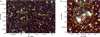 |
Fig. 4 Panel a: NIR color composite image of the region associated with the H II regions using VVV JHK bandimages (red – K; green – H; blue – J). “×” marks show the location of the H II regions. Panel b: zoomed in view of indicated region related to G346.077−0.056. The yellow circle denotes the size of the cluster as estimated by Borissova et al. (2011). The cyan contours show the higher-resolution 1280 MHz radio emission with the levels same as those plotted in Fig. 2. |
Details of the candidate ionizing star(s) for the H II regions.
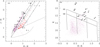 |
Fig. 5 Panel a: (J−H) vs (H−K) CCP for the region associated with the H II regions. The loci of main sequence (thin line) and giants (thick line) are taken from Bessell & Brett (1988). The classical T Tauri locus (long dashed line) is adopted from Meyer et al. (1997) and that for the Herbig AeBe stars (short dashed line) is from Lada & Adams (1992). The parallel lines are thereddening vectors where cross marks indicate intervals of 5 mag of visual extinction. The interstellar reddening law assumed is from Rieke & Lebofsky (1985). The colors and curves in the CCP are all converted into Bessell & Brett (1988) system. The regions “F”, “T”, and “P” are discussed in the text. The dotted line parallel to the reddening vector accounting for an offset of three times the photometric error in the bands. On the CCP, the Class I sources (blue) and Class II sources (red) are shown as filled circles. The candidate ionizing stars are shown as filled black circles (for G346.056−0.021) and open circles (for G346.077−0.056) on both CCP and CMP. The individual error bars on the colors and magnitude are also plotted. Panel b: K vs (H−K) CMP for the region associated with the H II regions. The nearly vertical solid lines represent the ZAMS loci with 0, 10, 20 and 30 magnitudes of visual extinction corrected for the distance. The slanting lines show the reddening vectors for spectraltypes O9 and O5. The magnitudes and the ZAMS loci are all plotted in the Bessell & Brett (1988) system. |
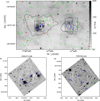 |
Fig. 6 Panel a: distribution of candidate ionizing stars and YSOs on the Spitzer 8.0 μm image. Identified YSOs have the following color coding – Class I (red), Class II (green). The ionizing stars are shown in blue. The detected clump apertures (see Sect. 3.3) are displayed in black. 1280 MHz (low resolution) radio contours are overlaid with levels of 3, 9, 13, 25, 30, 40, and 50 times σ. Panels b and c: zooms of regions (marked as black rectangles in panel a) associated with G346.077−0.056 and G346.056−0.021, respectively, on the K-band VVV image. In panel b, we have overlaid the high-resolution 1280 MHz radio contours shown in Fig. 2 to reveal the finer structures. |
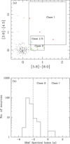 |
Fig. 7 Panel a: IRAC color-color plot for the sources in the H IIregions. The boxes demarcate the location of Class I (larger box)and Class II (smaller box) (Vig et al. 2007). Sources falling in the overlapping area are designated as Class I/II. The identified YSOs have the following color coding - Class I (red), Class II (green) and Class I/II (cyan). Panel b: histogram showing the number of sources within specified spectral index bins. The regions demarcated on the plot are adopted from Chavarría et al. (2008) for classification of YSOs. |
3.3 Emission from dust component
Figure 8 shows the MIR and FIR emission sampled in the IRAC, MIPSGAL, and Hi-Gal images. Diffuse emission is seen towards the H II regions in all four IRAC bands. As discussed in Watson et al. (2008), various processes contribute to the emission in each IRAC band. These include thermal emission from the circumstellar dust heated by the stellar radiation and emission due to excitation of polycyclic aromatic hydrocarbons (PAHs) by UV photonsin the Photo Dissociation Regions. In H II regions there would be significant contribution from trapped Lyα heated dust as well (Hoare et al. 1991). Apart from this, diffuse emission in the Brα and Pfβ lines and H2 line emission from shocked gas would also exist (Watson et al. 2008). The shorter IRAC bands (3.6, 4.5 μm) reveal the point sources, since emission here is dominated by the stellar photosphere. As seen in the figure, the two H II regions show up as faint, compact nebulosities. The extent and brightness of the diffuse emission increases from 3.6 to 8.0 μm. Further, at 5.8 and 8.0 μm, G346.056−0.021 shows an extended bubble-type morphology towards the south-west. G346.077−0.056 shows an extended, diffuse morphology with an irregular distribution of MIR emission (see Fig. 11). This will be discussed in more detail in a later section. The comparison of the [5.8] band, which is mostly a dust tracer, and the [4.5] band, which has significant contribution from Brα emission (H+ tracer; Churchwell et al. 2004) shows that the two H IIregions are dominated by dust emission. The 24 μm emission is in unison with the radio free-free emission. This emission which spatially correlates well with the ionized component can be attributed to Lyα heating of normal-size dust grains that could maintain the temperatures close to 100 K in the ionized region (Hoare et al. 1991). Few authors also associate the 24 μm emission in H II regions with either Very Small Grains or Big Grain replenishment (Everett & Churchwell 2010; Paladini et al. 2012). As we move towards the cold dust sampled with the Herschel bands, filamentary structures are prominent and seem to connect the two H II regions. The extent and brightness of G346.056−0.021 decreases and that of G346.077−0.056 increases as we go longward of 160 μm suggesting the dominance of warm dust in G346.056−0.021 and cold dust in G346.077−0.056.
We study the nature of the cold dust emission using the Herschel FIR bands. Line-of-sight average molecular hydrogen column density and dust temperature maps are generated by pixel-wise modified single temperature blackbody fits using the background-corrected fluxes and assuming the emission at these wavelengths to be optically thin. As discussed and adopted in several studies (Peretto et al. 2010; Anderson et al. 2010; Battersby et al. 2011; Liu et al. 2016), we have also excluded the 70 μm emission. This is because the emission at 70 μm may not be optically thin. Apart from this, there would be significant contribution from warm dust components and hence the SED cannot be modeled with a single-temperature graybody. Thus we have only four points, mostly on the Raleigh-Jeans part, to constrain the model.
The first step involves converting the SPIRE map units from MJy sr−1 to Jy pixel−1 which is the unit of the PACS images. Subsequently, the 70, 160, 250, and 350 μm images are convolved and regridded to the lowest resolution (35.7′′) and largest pixel size (14′′) of the 500 μm image. The convolution kernels are taken from Aniano et al. (2011). The above steps are carried out using the Herschel data reduction software HIPE3 .
We have estimated the background flux, I bg , in each band from a relatively smooth and dark region devoid of bright diffuse emission and filamentary structures. This region is located at an angular distance of ~ 1° from the H II regions and centered at α2000 = 17:11:57.17, δ2000 = −41:06:38.99. The background value was estimated by fitting a Gaussian function to the distribution of individual pixels in the specified region. The fitting was carried out iteratively by rejecting the pixels with values outside ±2σ till the fit converged (Battersby et al. 2011; Launhardt et al. 2013). We have used the same region for the determination of background offset in all the bands. I bg is estimated to be −3.22, 1.45, 0.72, and 0.26 Jy pixel−1 at 160, 250, 350, and 500 μm, respectively. The negative flux value at 160 μm is due to the arbitrary scaling of the PACS images.
The pixel-to-pixel SED fitting was carried out by adopting the following expressions (Battersby et al. 2011; Faimali et al. 2012; Launhardt et al. 2013; Mallick et al. 2015).
 (8)
(8)
where, Sν(ν) is the observed flux density, Ibg(ν) is the background flux, Bν(ν, Td) is the Planck’s function, Td is the dust temperature, Ω is the solid angle (in steradians) from where the flux is obtained (solid angle subtended by a 14″× 14″ pixel),  is the mean molecular weight, mH is the mass of hydrogen atom, κν is the dust opacity and N(H2) is the column density. We have assumed a value of 2.8 for
  (Kauffmann et al. 2008). The dust opacity κν is defined to be
  , where, β is the dust emissivity spectral index (Hildebrand 1983; Beckwith et al. 1990; André et al. 2010). The above model was fitted to the four data points using the non-linear least square Levenberg–Marquardt algorithm, where Td and N(H2) are kept as free parameters. Given the limited number of data points, we prefer to fix the value of β to 2 (Hildebrand 1983; Beckwith et al. 1990; André et al. 2010) which is also a typical value estimated for a large sample of H II regions (Anderson et al. 2012). We have used a conservative 15% uncertainty on the background-subtracted flux densities (Launhardt et al. 2013). The generated column density, dust temperature maps, and the corresponding χ2 map are shown in Fig. 9. We have overlaid the 1280 MHz radio map to correlate the emission from ionized gas and the cold dust component. The fitting uncertainties are small as is evident from the χ2 map where the maximum value for individual pixel fits is ~ 1.
The column density map shows a large clump enveloping the H II region G346.077−0.056 with the previously mentioned western filamentary structure visible. The region associated with G346.056−0.021 shows relatively low column density which is indicative of a less significant cold dust component. The peak (5.9 × 1022 cm−2) is located close to the radio peak of G346.077−0.056. Apart from the H II regions, a compact, spherical clump is seen to the south of G346.077−0.056. The association of this clump with the H II regions is not certain as there is no supporting literature available. As expected, we see regions of higher dust temperature toward both the H II regions. The dust temperature map shows extended warm distribution towards the north-east of G346.056−0.021 with the dust temperature distribution peaking just north of G346.056−0.021. This extended distribution coincides with a faint diffuseionized structure (detected at the 3σ level of the 1280 MHz emission). The southern compact clump displays the coldest dust temperature.
To identify and study the cold dust clumps, we use the ATLASGAL 870 μm map because this wavelength is sensitive to the colder dust components and also the emission is optically thin. Further, the resolution of the ATLASGAL map is better (18. ′′2) compared to the column density map (35′′.7). We use the two-dimensional (2D) Clumpfind algorithm (Williams et al. 1994) with a 2σ (where, σ = 0.06 Jy beam−1) threshold and optimum contour levels to detect the clumps. Using this threshold three clumps are detected, the retrieved apertures of which are shown overlaid on the ATLASGAL image in Fig. 10. Clump 1 overlaps with the southern part of the H II region G346.056−0.021 and is mostly part of the filamentary structure. Clump 2 is seen to be associated and enveloping G346.077−0.056. Clump 3 is located towards the south of G346.077−0.056. Masses of the clumps are estimated using the following expression
 (10)where mH is the mass of hydrogen, Apixel is the pixel area in cm2,
  is the mean molecular weight and ΣN(H2) is the integrated column density over the pixel area. Clump apertures retrieved from the Clumpfind algorithm are used to determine ΣN(H2) from the column density map. Location of 870 μm peaks, deconvolved sizes, mean dust temperature, mean column density, integrated column density, masses and number density (
 , r being the radius) of the clumps are estimated and listed in Table 5. Clump 2 has been studied by Yu et al. (2015). They have estimated the mass of the clump from 870 μm integrated flux density. Assuming a dust temperature of 30 K, they obtain a mass of 13 013 M⊙. This is a factor of ~1.2 lower than the estimates from our column density map. The possible reason for the higher mass estimate in our work could be the lower dust temperature (21 K) and different dust opacity assumed. One also cannot exclude the effect of flux loss associated with ground-based observations (Liu et al. 2017).
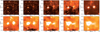 |
Fig. 8 Dust emission associated with the H II regions is shown: top panel from left 3.6, 4.5, 5.8, 8.0, 24 μm ; bottom panel from left 70, 160, 250, 350, 500 μm. The “×” marks are the positions of the H II regions. The “+” mark shows the position of the associated IRAS point source, IRAS 17043−4027. |
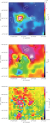 |
Fig. 9 Column density (panel a), dust temperature (panel b) and chi-square (χ2 ) (panel c) maps of the region associated to H II regions. 1280 MHz GMRT radio emission is shown as contours. The contour levels are same as those plotted in Fig. 6. The dashed line on the H II regions shows the projections, the column density variation which is used to understand the morphology of the ionized region in a later section. |
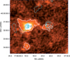 |
Fig. 10 ATLASGAL image shown, on top of which the clump apertures are overlaid. The clumps are labeled as 1, 2, and 3. 1280 MHz GMRT radio emission is shown as cyan contours with the same levels as those plotted in Fig. 6. |
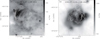 |
Fig. 11 1280 MHz radio contours overlaid on the 8.0 μm gray-scale image of panel a: G346.056−0.021 and panel b: G346.077−0.056. In panel a we have overlaid the lower-resolution contours presented inFig. 3 and in panel b to show the finer structures, we plot the higher-resolution contours as shown in Fig. 2. |
Physical parameters of the clumps.
4 Morphology of the H II regions
As mentioned in Sect. 3.1, both the H II regions show signature of cometary morphology in the radio. This morphology shows up as a bright, arc-type head and a diffuse, broad tail emission. In Fig. 11, we compare the radio morphology with the MIR emission in IRAC 8.0 μm band. The radio and MIR emission associated with G346.056−0.021 is seen to spatially correlate towards the head but there is a void in the MIR emission towards the tail implying that the H II region is density-bounded towards the south-west. The picture presented by G346.056−0.021 is similar tothat of the cometary H II region G331.1465+00.1343 shown in Fig. 1 of Hoare et al. (2007). In contrast, the MIR emission associated with G346.077−0.056 is extended and envelopes most of the ionized region. The radio peak and the possible second H II region is seen to coincide with the enhanced MIR emission towards the east.
In this section, we attempt to understand the origin of such cometary morphologies that are commonly seen in H II regions (Wood & Churchwell 1989). Several models have been proposed in the literature to address this, of which the frequently used ones are (i) the bow-shock model and (ii) the champagne-flow model. The former is due to the interaction of a supersonically moving, wind-blowing, ionizing star with the dense surrounding molecular gas. The latter model is a result of a steep density gradient encountered by an expanding H II region around a nearly stationary, ionizing source. Here, the ionizing star is possibly located at the edge of a dense clump where the ionized gas expands asymmetrically out towards regions of minimum density. Initial papers by Reid & Ho (1985), van Buren et al. (1990), Mac Low et al. (1991), Israel (1978),Tenorio-Tagle (1979) offer a detailed insight into these two models and the related physical conditions favoring one over the other. Recently, more involved radiation-hydrodynamic models have been proposed that include density gradient in the surrounding medium and a stellar wind contribution from an ionizing star in addition to its supersonic motion within the ambient cloud (Arthur & Hoare 2006). Another recent paper by Roth et al. (2014) explores a quasi-one-dimensional, steady-state wind model to explain the cometary morphology of UCH II regions. High spatial and spectral resolution observations of the MIR [Ne II] fine structure line in a sample of H II and UCH II regions by Zhu et al. (2005), Zhu et al. (2008) have shed further light on the various models. These studies show the co-existence of H II regions with dense and massive molecular cores where the ionized emission displays parabolic shells with the open end facing away from the dense cores and the kinematics reveal gas flow tangential to these shells. RRL studies of cometary H II regions have also invoked “hybrid” (combination of bow-shock and champagne-flow) models to explain the observed velocity structure (Immer et al. 2014).
Based on simple analytic expressions and arguments, we aim at interpreting the observed morphology of the ionized emission and the column density distribution associated with our H II regions. We first consider the bow-shock model and derive the bow-shock parameters along the lines discussed in Reid & Ho (1985), van Buren et al. (1990), Mac Low et al. (1991). In this model, the stellar wind freely streams in all directions until it encounters a terminal shock. In the direction of motion, the shock occurs at a distance ls (stand-off-distance) from the star, where the momentum flux of the wind equals ram pressure of the surrounding ambient ISM. This “bow-shock” gives rise to a H II region resembling a thin paraboloidal shell in the plane of the sky.
The stand-of distance ls is estimated using the following expressions (van Buren et al. 1990; Mac Low et al. 1991)
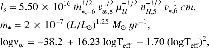 (11) (12) (13)
where ṁ*,−6 = ṁ* × 106 M⊙ yr−1 is the stellar wind mass-loss rate, vw,8 = vw × 108 cm s−1 is the terminal velocity of the wind, μH is the mean mass per hydrogen nucleus, nH,5 = nH × 105 cm−3 is the hydrogen gas density, v*,6 = v* × 106 cm s−1 is the relative velocity of star, L and L⊙ are the luminosity of star and sun, respectively, and Teff is the effective temperature of the star. The medium through which the star moves would be a combination of ionized and neutral medium. We consider a neutral medium here and take μH = 1.4 mH, where mH is taken as one atomic mass unit. We estimate nH to be 6.2 × 104 cm−3 and 4.8 × 104 cm−3 for G346.056−0.021 and G346.077−0.056, respectively, from the column density maps (refer Sect. 3.3). For the estimated spectral type of the ionizing stars, we assume luminosities in the range 1.0 × 10⁵-1.3 × 10⁵L⊙ and 6.6 × 10⁴-8.0 × 10⁴L⊙ for G346.056−0.021 and G346.077−0.056, respectively,from Martins et al. (2005). We further assume a typical velocity of 10 km s−1 (van Buren & Mac Low 1992) for the ionizing star. Plugging in these values in the above equations, we calculatethe expected stand-off distances. For G346.056−0.021 we obtain a value of 0.4′′(0.02 pc)–0.5′′(0.03 pc) and for G346.077−0.056 we estimate 0.2′′(0.01 pc)–0.3′′(0.016 pc). In the image plane, the stand-off distance is defined as the distance between the steep density gradient at the cometary head and the radio peak (assuming this to be the location of the ionizing star). Hence from the radio maps, we estimate ls to be ~9′′(0.5pc) and ~11′′(0.6pc) for G346.056−0.021 and G346.077−0.056, respectively.These values are significantly larger than the expected theoretical values. The discrepancies between the theoretical and observed stand-off distance estimates narrows down if we consider ionizing stars to move slower, with a velocity of ~ 1 km s−1. It should be noted here that the ionizing star need not always be at the location of the radio peak (Martín-Hernández et al. 2003) and that the viewing angle would also play a role in the estimated stand-off distance.
Further light can be shed by deriving the trapping parameter (τbs). As discussed in Mac Low et al. (1991), the dense shells swept up by the supersonically moving, ionizing star trap the H II region and the ram pressure inhibits their further dynamical expansion. This parameter is so defined that its inverse gives the ionization fraction. The shell thus traps the H IIregion when there are more recombinations in the shell compared to ionizing photons. This happens when τbs > 1. This parameter is shown to be much larger (τbs >> 1) as computed by Mac Low et al. (1991) for a sample of cometary H II regions. We estimate τbs for G346.056−0.021 and G346.077−0.056 using the following expression from Mac Low et al. (1991)
 (14)
(14)
where TII = TII,4 × 104 is the temperature of ionized gas, N ly = Nly49 × 1049 is the ionizing photon flux, γ is the ratio between specific heats, α is the hydrogen recombination rate to all levels but the ground state, given in units of 10−13cm3 s−1, and Nly is 3.2 × 1048 photons s−1 and 1.6 × 1048 photons s−1 for G346.056−0.021 and G346.077−0.056, respectively (refer Sect. 3.1). The temperature of ionized gas is 5500 K and 8900 K for G346.056−0.021 and G346.077−0.056, respectively, and the value of γ is 5/3. The value of α is estimated to be 4.3 × 10⁻¹³ cm3 s−1 and 3.0 × 10⁻¹³ cm3 s−1 at 5500 K and 8900 K, respectively, by a linear interpolation of the optically thick case from Osterbrock (1989). The derived values of τbs lie in the range 4.3–2.7 and 1.8–1.2 for G346.056−0.021 and G346.077−0.056, respectively. These values suggest weak or no bow shock.
Considering the above, it is less likely that the bow-shock mechanism is in play in G346.056−0.021 and G346.077−0.056. Given this, we explore the alternate model of champagne flow. Here, the morphology of the H II region is mostly dictated by the density structure of the molecular cloud. The H II region expands preferentially toward low-density regions resulting in a champagne flow. To probe this, we try to understand the variation in ionized emission and correlate with the column density distribution along the respective cometary axes which are marked in Fig. 9. We choose the 1280 MHz map. These projected lines also pass through the respective radio peaks of G346.056−0.021 and G346.077−0.056. The profiles are displayed in Fig. 12. Here, the x-axis shows the positional offset from the radio peak increasing towards the direction of the “tail”. The y-axis of the top panels which shows the variation in radio flux density is normalized to the peak values. In the bottom panels, the column density values are given in terms of 1022 cm−2. The ionized emission profiles are characteristic of cometary morphology (Wood & Churchwell 1989). What is interesting is the correlation with the density structure. As visible from the plots, the column density distribution peaks ahead of the ionized emission for both the regions implying that dense molecular gas is located at the head of the cometary arc of the H II regions which stalls the ionization front thus keeping the H II regions pressure and ionization bounded in the north-east and east directions for G346.056−0.021 and G346.077−0.056, respectively. On the other side, ionized gas streams away into the more rarefied environment which reveals itself as a decreasing column density distribution. These are signatures of a champagne flow. Thus it is likely that the cometary morphology is due to the density gradient rather than the supersonic motion of the ionizing star. It should be noted here that the above discussions are based on the projected morphology of the ionized and molecular gas where we have not considered the effect of viewing angle. One also has to keep in mind that the resolution and pixel sizes of the two maps used here are very different and hence crucial small-scale correlation is not possible. Though the analytical calculation based on simple assumptions do not present a strong case for a bow-shock scenario and the observed morphology agrees well with the champagne-flow model, it is necessary to study in detail the gas kinematics with the highest spectral and spatial resolution in order to understand the physical mechanism responsible for the cometary structure of the ionized regions.
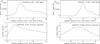 |
Fig. 12 Relative distribution of radio emission and column density with respect to the radio peaks for G346.056−0.021 and G346.077−0.056 along the projections shown in the column density map in Fig. 9. Zero on the x-axis corresponds to the position of the radio peaks increasing towards the direction of the tail (south-west for G346.056−0.021 and east for G346.077−0.056). The radio flux densities plotted are normalized to the peak flux densities and the column density is given in terms of 1022 cm −2. |
5 Summary
We have carried out a detailed study of the complex associated with the two southern galactic H II regions, G346.056−0.021 and G346.077−0.056. Based on our analysis we deduce the following.
-
Radio continuum emission is detected towards both H IIregions at 610 and 1280 MHz. The ionized emission morphology shows a cometary structure for G346.056−0.021. The morphology for G346.077−0.056 is mostly compact and spherical with a faint cometary signature.
-
The ZAMS spectral type of the ionizing sources are estimated to lie in the range O7.5V–O7V and O8.5V–O8V for G346.056−0.021 and G346.077−0.056, respectively. The dynamical ages of G346.056−0.021 and G346.077−0.056 are similar and estimated to be ~0.5–0.2 Myr.
-
Emission from the dust component shows cold dust to be predominantly located near G346.077−0.056 and the region associated with G346.056−0.021 contains relatively warmer dust. The column density map shows the presence of a dense clump towards G346.077−0.056. Two additional clumps are detected in the 870 μm image, one of which is towards G346.056−0.021.
-
Assuming the clumps to be physically associated and hence at the same distance, the masses are estimated to be 1922, 15 248, and 1412 M⊙ for clumps 1, 2, and 3, respectively, from the column density map.
-
Simple analytical calculations show that the bow-shock mechanism is less likely to be responsible for the observed cometary morphology. The variation of the ionized gas and the column density along the cometary axis favors the champagne-flow model for both H II regions.
Acknowledgements
We thank the referee for valuable comments and suggestions, which have helped to improve the quality of the paper. We thank the staff of the GMRT that made the radio observations possible. GMRT is run by the National Centre for Radio Astrophysics of the Tata Institute of Fundamental Research. This publication makes use of data products from the Two Micron All Sky Survey, which is a joint project of the University of Massachusetts and the Infrared Processing and Analysis Center/California Institute of Technology, funded by the NASA and the NSF. Point Source Catalog (PSC; Skrutskie et al. 2006)
References
- Allen, L. E., Calvet, N., D’Alessio, P., et al. 2004, ApJS, 154, 363 [NASA ADS] [CrossRef] [Google Scholar]
- Anderson, L. D., Zavagno, A., Rodón, J. A., et al. 2010, A&A, 518, L99 [NASA ADS] [CrossRef] [EDP Sciences] [Google Scholar]
- Anderson, L. D., Bania, T. M., Balser, D. S., & Rood, R. T. 2011, ApJS, 194, 32 [NASA ADS] [CrossRef] [Google Scholar]
- Anderson, L. D., Zavagno, A., Deharveng, L., et al. 2012, A&A, 542, A10 [NASA ADS] [CrossRef] [EDP Sciences] [Google Scholar]
- Anderson, L. D., Hough, L. A., Wenger, T. V., Bania, T. M., & Balser, D. S. 2015, ApJ, 810, 42 [NASA ADS] [CrossRef] [Google Scholar]
- André, P., Men’shchikov, A., Bontemps, S., et al. 2010, A&A, 518, L102 [NASA ADS] [CrossRef] [EDP Sciences] [Google Scholar]
- Aniano, G., Draine, B. T., Gordon, K. D., & Sandstrom, K. 2011, PASP, 123, 1218 [NASA ADS] [CrossRef] [Google Scholar]
- Arthur, S. J., & Hoare, M. G. 2006, ApJS, 165, 283 [NASA ADS] [CrossRef] [Google Scholar]
- Arthur, S. J., Kurtz, S. E., Franco, J., & Albarrán, M. Y. 2004, ApJ, 608, 282 [NASA ADS] [CrossRef] [Google Scholar]
- Battersby, C., Bally, J., Ginsburg, A., et al. 2011, A&A, 535, A128 [NASA ADS] [CrossRef] [EDP Sciences] [Google Scholar]
- Beckwith, S. V. W., Sargent, A. I., Chini, R. S., & Guesten, R. 1990, AJ, 99, 924 [NASA ADS] [CrossRef] [Google Scholar]
- Benjamin, R. A., Churchwell, E., Babler, B. L., et al. 2003, PASP, 115, 953 [NASA ADS] [CrossRef] [Google Scholar]
- Bessell, M. S., & Brett, J. M. 1988, PASP, 100, 1134 [NASA ADS] [CrossRef] [Google Scholar]
- Borissova, J., Bonatto, C., Kurtev, R., et al. 2011, A&A, 532, A131 [NASA ADS] [CrossRef] [EDP Sciences] [Google Scholar]
- Bronfman, L., Nyman, L.-A., & May, J. 1996, A&AS, 115, 81 [NASA ADS] [Google Scholar]
- Carey, S. J., Noriega-Crespo, A., Mizuno, D. R., et al. 2009, PASP, 121, 76 [NASA ADS] [CrossRef] [Google Scholar]
- Caswell, J. L., Fuller, G. A., Green, J. A., et al. 2010, MNRAS, 404, 1029 [NASA ADS] [CrossRef] [Google Scholar]
- Chavarría, L. A., Allen, L. E., Hora, J. L., Brunt, C. M., & Fazio, G. G. 2008, ApJ, 682, 445 [NASA ADS] [CrossRef] [Google Scholar]
- Churchwell, E. 2002, ARA&A, 40, 27 [Google Scholar]
- Churchwell, E., Whitney, B. A., Babler, B. L., et al. 2004, ApJS, 154, 322 [NASA ADS] [CrossRef] [Google Scholar]
- Das, S. R., Tej, A., Vig, S., et al. 2017, MNRAS, 472, 4750 [NASA ADS] [CrossRef] [Google Scholar]
- Davies, B., Hoare, M. G., Lumsden, S. L., et al. 2011, MNRAS, 416, 972 [NASA ADS] [CrossRef] [Google Scholar]
- Dyson, J. E., & Williams, D. A. 1980, Physics of the Interstellar Medium [Google Scholar]
- Everett, J. E.,& Churchwell, E. 2010, ApJ, 713, 592 [NASA ADS] [CrossRef] [Google Scholar]
- Faimali, A., Thompson, M. A., Hindson, L., et al. 2012, MNRAS, 426, 402 [NASA ADS] [CrossRef] [Google Scholar]
- Fazio, G. G., Hora, J. L., Allen, L. E., et al. 2004, ApJS, 154, 10 [NASA ADS] [CrossRef] [Google Scholar]
- Froebrich, D. 2013, Int. J. Astron. Astrophys., 3, 161 [CrossRef] [Google Scholar]
- Garay, G., & Lizano, S. 1999, PASP, 111, 1049 [NASA ADS] [CrossRef] [Google Scholar]
- Griffin, M. J., Abergel, A., Abreu, A., et al. 2010, A&A, 518, L3 [Google Scholar]
- Hildebrand, R. H. 1983, QJRAS, 24, 267 [NASA ADS] [Google Scholar]
- Hoare, M. G., Roche, P. F., & Glencross, W. M. 1991, MNRAS, 251, 584 [NASA ADS] [Google Scholar]
- Hoare, M. G., Kurtz, S. E., Lizano, S., Keto, E., & Hofner, P. 2007, Protostars and Planets V, 181 [Google Scholar]
- Hoq, S., Jackson, J. M., Foster, J. B., et al. 2013, ApJ, 777, 157 [NASA ADS] [CrossRef] [Google Scholar]
- Immer, K., Cyganowski, C., Reid, M. J., & Menten, K. M. 2014, A&A, 563, A39 [NASA ADS] [CrossRef] [EDP Sciences] [Google Scholar]
- Inoue, A. K., Hirashita, H., & Kamaya, H. 2001, ApJ, 555, 613 [NASA ADS] [CrossRef] [Google Scholar]
- Israel, F. P. 1978, A&A, 70, 769 [NASA ADS] [Google Scholar]
- Kauffmann, J., Bertoldi, F., Bourke, T. L., Evans, II, N. J., & Lee, C. W. 2008, A&A, 487, 993 [NASA ADS] [CrossRef] [EDP Sciences] [Google Scholar]
- Kobulnicky, H. A., & Johnson, K. E. 1999, ApJ, 527, 154 [NASA ADS] [CrossRef] [Google Scholar]
- Kwan, J. 1997, ApJ, 489, 284 [NASA ADS] [CrossRef] [Google Scholar]
- Lada, C. J. 1987, in Star Forming Regions, eds. M. Peimbert & J. Jugaku, IAU Symp., 115, 1 [NASA ADS] [CrossRef] [Google Scholar]
- Lada, C. J., & Adams, F. C. 1992, ApJ, 393, 278 [NASA ADS] [CrossRef] [Google Scholar]
- Lal, D. V., & Rao, A. P. 2007, MNRAS, 374, 1085 [NASA ADS] [CrossRef] [Google Scholar]
- Launhardt, R., Stutz, A. M., Schmiedeke, A., et al. 2013, A&A, 551, A98 [NASA ADS] [CrossRef] [EDP Sciences] [Google Scholar]
- Liu, H.-L., Li, J.-Z., Wu, Y., et al. 2016, ApJ, 818, 95 [NASA ADS] [CrossRef] [Google Scholar]
- Liu, H.-L., Figueira, M., Zavagno, A., et al. 2017, A&A, 602, A95 [NASA ADS] [CrossRef] [EDP Sciences] [Google Scholar]
- Luisi, M., Anderson, L. D., Balser, D. S., Bania, T. M., & Wenger, T. V. 2016, ApJ, 824, 125 [NASA ADS] [CrossRef] [Google Scholar]
- Lumsden, S. L., Hoare, M. G., Urquhart, J. S., et al. 2013, ApJS, 208, 11 [NASA ADS] [CrossRef] [Google Scholar]
- Mac Low, M.-M., van Buren, D., Wood, D. O. S., & Churchwell, E. 1991, ApJ, 369, 395 [NASA ADS] [CrossRef] [Google Scholar]
- Mallick, K. K., Ojha, D. K., Tamura, M., et al. 2015, MNRAS, 447, 2307 [NASA ADS] [CrossRef] [Google Scholar]
- Martín-Hernández, N. L., Bik, A., Kaper, L., Tielens, A. G. G. M., & Hanson, M. M. 2003, A&A, 405, 175 [NASA ADS] [CrossRef] [EDP Sciences] [Google Scholar]
- Martins, F., Schaerer, D., & Hillier, D. J. 2005, A&A, 436, 1049 [NASA ADS] [CrossRef] [EDP Sciences] [Google Scholar]
- Meyer, M. R., Calvet, N., & Hillenbrand, L. A. 1997, AJ, 114, 288 [NASA ADS] [CrossRef] [Google Scholar]
- Mezger, P. G., & Henderson, A. P. 1967, ApJ, 147, 471 [NASA ADS] [CrossRef] [Google Scholar]
- Minniti, D., Lucas, P. W., Emerson, J. P., et al. 2010, New A, 15, 433 [Google Scholar]
- Molinari, S., Swinyard, B., Bally, J., et al. 2010, A&A, 518, L100 [NASA ADS] [CrossRef] [EDP Sciences] [Google Scholar]
- Morales, E. F. E., Wyrowski, F., Schuller, F., & Menten, K. M. 2013, A&A, 560, A76 [NASA ADS] [CrossRef] [EDP Sciences] [Google Scholar]
- Mottram, J. C., Hoare, M. G., Davies, B., et al. 2011, ApJ, 730, L33 [NASA ADS] [CrossRef] [Google Scholar]
- Mücke, A., Koribalski, B. S., Moffat, A. F. J., Corcoran, M. F., & Stevens, I. R. 2002, ApJ, 571, 366 [NASA ADS] [CrossRef] [Google Scholar]
- Nandakumar, G., Veena, V. S., Vig, S., et al. 2016, AJ, 152, 146 [NASA ADS] [CrossRef] [Google Scholar]
- Ojha, D. K., Tamura, M., Nakajima, Y., et al. 2004a, ApJ, 608, 797 [NASA ADS] [CrossRef] [Google Scholar]
- Ojha, D. K., Tamura, M., Nakajima, Y., et al. 2004b, ApJ, 616, 1042 [NASA ADS] [CrossRef] [Google Scholar]
- Osterbrock, D. E. 1989, Astrophysics of Gaseous Nebulae and Active Galactic Nuclei (Mill Valley; University Science Books) [Google Scholar]
- Paladini, R., Umana, G., Veneziani, M., et al. 2012, ApJ, 760, 149 [NASA ADS] [CrossRef] [Google Scholar]
- Panagia, N. 1973, AJ, 78, 929 [NASA ADS] [CrossRef] [Google Scholar]
- Paron, S., Petriella, A., & Ortega, M. E. 2011, A&A, 525, A132 [NASA ADS] [CrossRef] [EDP Sciences] [Google Scholar]
- Peretto, N., Fuller, G. A., Plume, R., et al. 2010, A&A, 518, L98 [NASA ADS] [CrossRef] [EDP Sciences] [Google Scholar]
- Poglitsch, A., Waelkens, C., Geis, N., et al. 2010, A&A, 518, L2 [NASA ADS] [CrossRef] [EDP Sciences] [Google Scholar]
- Quireza, C., Rood, R. T., Bania, T. M., Balser, D. S., & Maciel, W. J. 2006, ApJ, 653, 1226 [NASA ADS] [CrossRef] [Google Scholar]
- Ranjan Das, S., Tej, A., Vig, S., Ghosh, S. K., & Ishwara Chandra C. H. 2016, AJ, 152, 152 [NASA ADS] [CrossRef] [Google Scholar]
- Reid, M. J., & Ho, P. T. P. 1985, ApJ, 288, L17 [NASA ADS] [CrossRef] [Google Scholar]
- Rieke, G. H., & Lebofsky, M. J. 1985, ApJ, 288, 618 [NASA ADS] [CrossRef] [Google Scholar]
- Rodriguez, L. F., Marti, J., Canto, J., Moran, J. M., & Curiel, S. 1993, Rev. Mex. Astron. Astrofis., 25, 23 [NASA ADS] [Google Scholar]
- Rosero, V., Hofner, P., Claussen, M., et al. 2016, ApJS, 227, 25 [NASA ADS] [CrossRef] [Google Scholar]
- Roth, N., Stahler, S. W., & Keto, E. 2014, MNRAS, 438, 1335 [NASA ADS] [CrossRef] [Google Scholar]
- Rubin, R. H. 1968, ApJ, 153, 761 [NASA ADS] [CrossRef] [Google Scholar]
- Russeil, D., Tigé, J., Adami, C., et al. 2016, A&A, 587, A135 [NASA ADS] [CrossRef] [EDP Sciences] [Google Scholar]
- Sánchez-Monge, Á., Kurtz, S., Palau, A., et al. 2013, ApJ, 766, 114 [NASA ADS] [CrossRef] [Google Scholar]
- Schmiedeke, A., Schilke, P., Möller, T., et al. 2016, A&A, 588, A143 [NASA ADS] [CrossRef] [EDP Sciences] [Google Scholar]
- Schraml, J., & Mezger, P. G. 1969, ApJ, 156, 269 [NASA ADS] [CrossRef] [Google Scholar]
- Schuller, F., Menten, K. M., Contreras, Y., et al. 2009, A&A, 504, 415 [NASA ADS] [CrossRef] [EDP Sciences] [Google Scholar]
- Skrutskie, M. F., Cutri, R. M., Stiening, R., et al. 2006, AJ, 131, 1163 [NASA ADS] [CrossRef] [Google Scholar]
- Spitzer, L. 1978, Physical Processes in the Interstellar Medium (New York: Wiley Interscience) [Google Scholar]
- Sugitani, K., Tamura, M., Nakajima, Y., et al. 2002, ApJ, 565, L25 [NASA ADS] [CrossRef] [Google Scholar]
- Swarup, G., Ananthakrishnan, S., Kapahi, V. K., et al. 1991, No.2/JAN25, P. 95, Curr. Sci., 60, 95 [Google Scholar]
- Tej, A., Ojha, D. K., Ghosh, S. K., et al. 2006, A&A, 452, 203 [NASA ADS] [CrossRef] [EDP Sciences] [Google Scholar]
- Tenorio-Tagle,G. 1979, A&A, 71, 59 [NASA ADS] [Google Scholar]
- Urquhart, J. S., Figura, C. C., Moore, T. J. T., et al. 2014, MNRAS, 437, 1791 [NASA ADS] [CrossRef] [Google Scholar]
- Urquhart, J. S., Busfield, A. L., Hoare, M. G., et al. 2007a, A&A, 461, 11 [NASA ADS] [CrossRef] [EDP Sciences] [Google Scholar]
- Urquhart, J. S., Busfield, A. L., Hoare, M. G., et al. 2007b, A&A, 474, 891 [NASA ADS] [CrossRef] [EDP Sciences] [Google Scholar]
- van Buren, D., & Mac Low M.-M. 1992, ApJ, 394, 534 [NASA ADS] [CrossRef] [Google Scholar]
- van Buren, D., Mac Low, M.-M., Wood, D. O. S., & Churchwell, E. 1990, ApJ, 353, 570 [NASA ADS] [CrossRef] [Google Scholar]
- van der Walt, D. J., Gaylard, M. J., & MacLeod, G. C. 1995, A&AS, 110, 81 [NASA ADS] [Google Scholar]
- Veena, V. S., Vig, S., Tej, A., et al. 2016, MNRAS, 456, 2425 [NASA ADS] [CrossRef] [Google Scholar]
- Vig, S., Ghosh, S. K., Ojha, D. K., & Verma, R. P. 2007, A&A, 463, 175 [NASA ADS] [CrossRef] [EDP Sciences] [Google Scholar]
- Watson, C., Povich, M. S., Churchwell, E. B., et al. 2008, ApJ, 681, 1341 [NASA ADS] [CrossRef] [Google Scholar]
- Wenger, T. V., Bania, T. M., Balser, D. S., & Anderson, L. D. 2013, ApJ, 764, 34 [NASA ADS] [CrossRef] [Google Scholar]
- Williams, J. P., de Geus, E. J., & Blitz, L. 1994, ApJ, 428, 693 [NASA ADS] [CrossRef] [Google Scholar]
- Wood, D. O. S., & Churchwell, E. 1989, ApJS, 69, 831 [NASA ADS] [CrossRef] [Google Scholar]
- Yu, N., Wang, J.-J., & Li, N. 2015, MNRAS, 446, 2566 [NASA ADS] [CrossRef] [Google Scholar]
- Zhang, C. P., & Wang, J. J. 2012, A&A, 544, A11 [NASA ADS] [CrossRef] [EDP Sciences] [Google Scholar]
- Zhu, Q.-F., Lacy, J. H., Jaffe, D. T., Richter, M. J., & Greathouse, T. K. 2005, ApJ, 631, 381 [NASA ADS] [CrossRef] [Google Scholar]
- Zhu, Q.-F., Lacy, J. H., Jaffe, D. T., Richter, M. J., & Greathouse, T. K. 2008, ApJS, 177, 584 [NASA ADS] [CrossRef] [Google Scholar]
- Zoonematkermani, S., Helfand, D. J., Becker, R. H., White, R. L., & Perley, R. A. 1990, ApJS, 74, 181 [NASA ADS] [CrossRef] [Google Scholar]
All Tables
GMRT, ATCA (Urquhart et al. 2007a), and 1.4 GHz (Zoonematkermani et al. 1990) results.
All Figures
|
Fig. 1 Color composite image of the region associated with G346.056−0.021 and G346.077−0.056 using IRAC 8.0 μm band (see Sect. 2.2.2; blue), MIPS 24 μm (MIPSGAL Survey; Carey et al. 2009; green), and ATLASGAL 870 μm (see Sect. 2.2.4; red). Positions of the H II regions as listed in Anderson et al. (2011) are shown with the “×” symbols. The “+” symbol shows the position of IRAS 17043−4027. It should be noted here that a few pixels toward the central part of the 24 μm emission associated with G346.077−0.056 are saturated. |
| In the text | |
|
Fig. 2 Ionized emission associated with the H IIregions – panels a and b: 610 and 1280 MHz maps for the region associated with G346.056−0.021; panels c and d: 610 and 1280 MHz emission for the region around G346.077−0.056. The contourlevels are 3, 5, 10, 15, 20, 25, 30, and 35 times σ, where σ is equal to 0.3 mJy beam−1 and 0.2 mJybeam−1 at 610 MHz and 1280 MHz, respectively. Beam in each band is shown as filled ellipse. These maps are generated by setting the “robustness parameter” to −5 and withoutany uv tapering. |
| In the text | |
|
Fig. 3 Sameas in Fig. 2, but for maps generated with “robustness parameter” +1 and appropriate uv tapering to weigh down long baselines. The contour levels are 3, 5, 7, 11, 15, 20, 25, 30, 40, and 55 times σ where σ is 2.1 mJy beam−1 and 0.5 mJybeam−1 at 610 MHz and 1280 MHz, respectively. Beam in each band is shown as filled ellipse. |
| In the text | |
|
Fig. 4 Panel a: NIR color composite image of the region associated with the H II regions using VVV JHK bandimages (red – K; green – H; blue – J). “×” marks show the location of the H II regions. Panel b: zoomed in view of indicated region related to G346.077−0.056. The yellow circle denotes the size of the cluster as estimated by Borissova et al. (2011). The cyan contours show the higher-resolution 1280 MHz radio emission with the levels same as those plotted in Fig. 2. |
| In the text | |
|
Fig. 5 Panel a: (J−H) vs (H−K) CCP for the region associated with the H II regions. The loci of main sequence (thin line) and giants (thick line) are taken from Bessell & Brett (1988). The classical T Tauri locus (long dashed line) is adopted from Meyer et al. (1997) and that for the Herbig AeBe stars (short dashed line) is from Lada & Adams (1992). The parallel lines are thereddening vectors where cross marks indicate intervals of 5 mag of visual extinction. The interstellar reddening law assumed is from Rieke & Lebofsky (1985). The colors and curves in the CCP are all converted into Bessell & Brett (1988) system. The regions “F”, “T”, and “P” are discussed in the text. The dotted line parallel to the reddening vector accounting for an offset of three times the photometric error in the bands. On the CCP, the Class I sources (blue) and Class II sources (red) are shown as filled circles. The candidate ionizing stars are shown as filled black circles (for G346.056−0.021) and open circles (for G346.077−0.056) on both CCP and CMP. The individual error bars on the colors and magnitude are also plotted. Panel b: K vs (H−K) CMP for the region associated with the H II regions. The nearly vertical solid lines represent the ZAMS loci with 0, 10, 20 and 30 magnitudes of visual extinction corrected for the distance. The slanting lines show the reddening vectors for spectraltypes O9 and O5. The magnitudes and the ZAMS loci are all plotted in the Bessell & Brett (1988) system. |
| In the text | |
|
Fig. 6 Panel a: distribution of candidate ionizing stars and YSOs on the Spitzer 8.0 μm image. Identified YSOs have the following color coding – Class I (red), Class II (green). The ionizing stars are shown in blue. The detected clump apertures (see Sect. 3.3) are displayed in black. 1280 MHz (low resolution) radio contours are overlaid with levels of 3, 9, 13, 25, 30, 40, and 50 times σ. Panels b and c: zooms of regions (marked as black rectangles in panel a) associated with G346.077−0.056 and G346.056−0.021, respectively, on the K-band VVV image. In panel b, we have overlaid the high-resolution 1280 MHz radio contours shown in Fig. 2 to reveal the finer structures. |
| In the text | |
|
Fig. 7 Panel a: IRAC color-color plot for the sources in the H IIregions. The boxes demarcate the location of Class I (larger box)and Class II (smaller box) (Vig et al. 2007). Sources falling in the overlapping area are designated as Class I/II. The identified YSOs have the following color coding - Class I (red), Class II (green) and Class I/II (cyan). Panel b: histogram showing the number of sources within specified spectral index bins. The regions demarcated on the plot are adopted from Chavarría et al. (2008) for classification of YSOs. |
| In the text | |
|
Fig. 8 Dust emission associated with the H II regions is shown: top panel from left 3.6, 4.5, 5.8, 8.0, 24 μm ; bottom panel from left 70, 160, 250, 350, 500 μm. The “×” marks are the positions of the H II regions. The “+” mark shows the position of the associated IRAS point source, IRAS 17043−4027. |
| In the text | |
|
Fig. 9 Column density (panel a), dust temperature (panel b) and chi-square (χ2 ) (panel c) maps of the region associated to H II regions. 1280 MHz GMRT radio emission is shown as contours. The contour levels are same as those plotted in Fig. 6. The dashed line on the H II regions shows the projections, the column density variation which is used to understand the morphology of the ionized region in a later section. |
| In the text | |
|
Fig. 10 ATLASGAL image shown, on top of which the clump apertures are overlaid. The clumps are labeled as 1, 2, and 3. 1280 MHz GMRT radio emission is shown as cyan contours with the same levels as those plotted in Fig. 6. |
| In the text | |
|
Fig. 11 1280 MHz radio contours overlaid on the 8.0 μm gray-scale image of panel a: G346.056−0.021 and panel b: G346.077−0.056. In panel a we have overlaid the lower-resolution contours presented inFig. 3 and in panel b to show the finer structures, we plot the higher-resolution contours as shown in Fig. 2. |
| In the text | |
|
Fig. 12 Relative distribution of radio emission and column density with respect to the radio peaks for G346.056−0.021 and G346.077−0.056 along the projections shown in the column density map in Fig. 9. Zero on the x-axis corresponds to the position of the radio peaks increasing towards the direction of the tail (south-west for G346.056−0.021 and east for G346.077−0.056). The radio flux densities plotted are normalized to the peak flux densities and the column density is given in terms of 1022 cm −2. |
| In the text | |
Current usage metrics show cumulative count of Article Views (full-text article views including HTML views, PDF and ePub downloads, according to the available data) and Abstracts Views on Vision4Press platform.
Data correspond to usage on the plateform after 2015. The current usage metrics is available 48-96 hours after online publication and is updated daily on week days.
Initial download of the metrics may take a while.