| Issue |
A&A
Volume 611, March 2018
|
|
|---|---|---|
| Article Number | A18 | |
| Number of page(s) | 18 | |
| Section | Planets and planetary systems | |
| DOI | https://doi.org/10.1051/0004-6361/201630175 | |
| Published online | 15 March 2018 | |
Local growth of dust- and ice-mixed aggregates as cometary building blocks in the solar nebula
1
Max Planck Institute for Solar System Research,
37077
Göttingen, Germany
e-mail: This email address is being protected from spambots. You need JavaScript enabled to view it.
2
Astrophysics Research Centre, Queen’s University Belfast,
Belfast
7 1NN, UK
3
Institut für Geophysik und extraterrestrische Physik, Technische Universität Braunschweig,
Mendelssohnstr. 3,
38106
Braunschweig, Germany
Received:
1
December
2016
Accepted:
22
November
2017
Abstract
Context. Comet formation by gravitational instability requires aggregates that trigger the streaming instability and cluster in pebble-clouds. These aggregates form as mixtures of dust and ice from (sub-)micrometre-sized dust and ice grains via coagulation in the solar nebula.
Aim. We investigate the growth of aggregates from (sub-)micrometre-sized dust and ice monomer grains. We are interested in the properties of these aggregates: whether they might trigger the streaming instability, how they compare to pebbles found on comets, and what the implications are for comet formation in collapsing pebble-clouds.
Methods. We used Monte Carlo simulations to study the growth of aggregates through coagulation locally in the comet-forming region at 30 au. We used a collision model that can accommodate sticking, bouncing, fragmentation, and porosity of dust- and ice-mixed aggregates. We compared our results to measurements of pebbles on comet 67P/Churyumov-Gerasimenko.
Results. We find that aggregate growth becomes limited by radial drift towards the Sun for 1 μm sized monomers and by bouncing collisions for 0.1 μm sized monomers before the aggregates reach a Stokes number that would trigger the streaming instability (Stmin). We argue that in a bouncing-dominated system, aggregates can reach Stmin through compression in bouncing collisions if compression is faster than radial drift. In the comet-forming region (~30 au), aggregates with Stmin have volume-filling factors of ~10−2 and radii of a few millimetres. These sizes are comparable to the sizes of pebbles found on comet 67P/Churyumov-Gerasimenko. The porosity of the aggregates formed in the solar nebula would imply that comets formed in pebble-clouds with masses equivalent to planetesimals of the order of 100 km in diameter.
Key words: protoplanetary disks / planets and satellites: formation / methods: numerical
© ESO 2018
1 Introduction
The comets we observe in the solar system stem from the population of kilometre-sized icy planetesimals that formed in the solar nebula beyond the snow line about 4.6 Gyr ago. Comets are highly porous objects (~70%–80% porosity Blum et al. 2006; Kofman et al. 2015; Fulle et al. 2016; Pätzold et al. 2016), and are composed of refractory dust and ices of different volatiles. Their bulk density is very low, about 0.5 g cm−3 (Blum et al. 2006; A’Hearn 2011; Sierks et al. 2015; Pätzold et al. 2016). However, we still lack detailed knowledge of the formation process of these fluffy objects. Two scenarios are currently under debate: 1) (porous) coagulation from (sub-)micrometre-sized dust and ice monomers to kilometre-sized planetesimals (e.g. Weidenschilling 1997; Okuzumi et al. 2012; Kataoka et al. 2013a), and 2) the gravitational instability of so-called pebble-clouds formed by the streaming instability (e.g. Youdin & Goodman 2005; Johansen et al. 2007). The term pebble refers to millimetre- to decimetre-sized aggregates and not to their dynamical behaviour. In this size range, however, aggregates develop significant drift with respect to the gas, which allows for the onset of the streaming instability. Both formation scenarios imply properties for the resulting bodies (e.g. tensile strength, density) that can be compared to the observed material properties of comets. Based on this, increasing evidence is piling up in favour of the pebble-cloud model for comet formation (Blum et al. 2014; Fulle & Blum 2017).
In the classical coagulation scenario, gas-drag-induced radial drift of aggregates towards the Sun, bouncing collisions, and fragmentation of aggregates prevent aggregates from growing beyond about centimetre in size (Weidenschilling 1977a; Blum & Wurm 2008; Güttler et al. 2010; Zsom et al. 2010). The sticking properties of water ice (Gundlach et al. 2011a; Gundlach & Blum 2015) and the formation of highly porous aggregates with densities ≲10−3 g cm−3 could, in principle, circumvent these limitations (Kataoka et al. 2013a). Porosity leads to accelerated growth through two effects. Firstly, the change of drag regime from Epstein to Stokes. The Stokes number is proportional to the aggregate size, a, in the Epstein regime and ∝ a2 in the Stokes regime. Therefore, a small increase in size leads to strong changes in aerodynamic behaviour, which slows down radial drift. Secondly, the collisional cross-section of porous aggregates is larger than for compact aggregates, which accelerates growth. These two effects combined make it possible to avoid the radial drift problem. Furthermore, the sticking property of water ice reduces the effect of fragmentation and allows for growing larger aggregates. However, this heavily relies on 0.1 μm ice monomers and a high threshold velocity for erosion and fragmentation (Okuzumi et al. 2012; Wada et al. 2013; Kataoka et al. 2013a; Krijt et al. 2015).
The basic idea of the gravitational instability model for comet formation is as follows (Blum et al. 2014; Wahlberg Jansson & Johansen 2014; Lorek et al. 2016; Wahlberg Jansson et al. 2017). The streaming instability leads to strong clustering of aggregates when certain criteria (Bai & Stone 2010; Carrera et al. 2015; Krijt et al. 2016; Yang et al. 2017) are met, namely: i) the aggregates have Stokes numbers (see Appendix A.2 for a definition) between 10−3 and 5; ii) the vertically integrated solid-to-gas ratio of the protoplanetary disk (hereafter metallicity, Z) is above a Stokes-number-dependent threshold, whose minimum is Z ≈ 0.015 for St ≈ 0.1; and iii) the mass loading of aggregates in the disk midplane exceeds unity, where the mass loading ρd ∕ρg is the ratio of dust (ρd) and gas density (ρg).
Once theaggregate clusters reach Roche density, they become gravitationally bound pebble-clouds. The subsequent gravitational collapse of the pebble-clouds, triggered by energy dissipation due to inelastic collisions, forms planetesimals with sizes ranging from a few kilometres up to a few hundred kilometres (Nesvorný et al. 2010; Wahlberg Jansson & Johansen 2014; Schäfer et al. 2017). This mechanism avoids the aforementioned limitations to growth and produces highly porous planetesimalswith tensile strengths consistent with those required to explain activity on comets (Skorov & Blum 2012; Blum et al. 2014). The high porosity obtained in this model is due to the combination of the aggregate porosity (volume-filling factor ≲0.4 Zsom et al. 2010, depending on the amount of collisional compression) and the random packing of the aggregates (volume-filling factor ~ 0.6 Skorov & Blum 2012; Fulle & Blum 2017). The porosity of the comet is thus about 70% to 80%, or higher if the aggregates are more porous. The gravitational collapse of the pebble-cloud can be described as a sequence of bouncing collisions of the aggregates. The low velocity at which the aggregates eventually stick (~ mm s−1) and the porosity of the aggregates result in a small contact area between them. Skorov & Blum (2012) showed that this leads to a tensile strength as low as ~ 1 Pa for millimetre-sized dust aggregates. In contrast, (porous) coagulation (of ice) produces more compact planetesimals (~ 60% porosity) with a significantly higher tensile strength (103 –104 Pa) (Blum et al. 2006, 2014) because the growth process is ballistic particle-cluster aggregation and the collision velocities are higher (~ m s −1 for mass transfer collisions), which produces rather compact aggregates (Kothe et al. 2010).
Lorek et al. (2016) studied the compression of centimetre-sized porous aggregates that is the result of bouncing collisions during the gravitational collapse of a pebble-cloud. Higher cloud masses lead to stronger compression because the collision speeds are higher. Lorek et al. (2016) used their results to constrain which combinations of initial aggregate properties (porosity, dust-to-ice ratio) and pebble-cloud masses would lead to planetesimals with densities in agreement with the measured bulk density of comets (0.5 g cm−3). Lorek et al. (2016) concluded that without further knowledge of the initial aggregate porosity, there are two indistinguishable ways to form comet-like planetesimals (see their Fig. 5): 1) collapse of clouds with masses corresponding to small (≲100 km) planetesimals and initially compact aggregates with volume-filling factor 0.4; and 2) collapse of more massive clouds, corresponding to large (≳100 km) planetesimals, regardless of initial aggregate porosity. In both cases the dust-to-ice ratio of the collapsed material must be in the range between 3 and 9 because aggregates with a dust-to-ice ratio in this range experience the right amount of compression such that the comet has a density of 0.5 g cm−3. Higher or lower dust-to-ice ratios result in stronger or weaker compressed aggregates and comets with higher or lower density (for a given random packing of aggregates). While the dust-to-ice ratio is broadly consistent with measurements of comets (e.g. Rotundi et al. 2015; Fulle 2017, who derived a value of ~5 for 67P/Churyumov-Gerasimenko), the initial aggregate porosity needs to be constrained from aggregate growth models to be able to distinguish between cases 1 and 2, respectively.
The main goal of this paper is to determine the properties of the aggregates that would be concentrated in pebble-clouds by the streaming instability and that would provide the building blocks of comets formed by the gravitational collapse of these clouds. We conduct simulations of aggregate growth from a two-component system of (sub-)micrometre-sized dust and ice monomers and address the question whether porous coagulation leads to aggregates with the right aerodynamic properties for streaming instability (e.g. Dra̧żkowska & Dullemond 2014; Krijt et al. 2015, 2016). We focus entirely on the Stokes number criterion for streaming instability and ignore conditions ii) and iii) mentioned above for the following reasons: Firstly, our current understanding of aggregate growth in the solar nebula shows that the formation of larger bodies is problematic because of growth-limiting processes (bouncing, fragmentation). Hence, it is important to study whether aggregates reach the minimum size for streaming instability at all. Secondly, we simulate aggregate growth in a vertically integrated model, which does not allow us to study particle concentration in the disk midplane other than through sedimentation. Sedimentation is in general not sufficient to produce condition iii) because turbulent diffusion puffs up the dust disk, resulting in a mass loading in the midplane ≪1. However, the turbulent motion of the protoplanetary disk gas passively concentrates dust in local pressure maxima through turbulent eddies, pressure bumps, or vortices. This should be sufficient to produce the initial situation of a mass loading ≳1 (Johansen et al. 2014). A detailed treatment, however, is beyond the scope of this work. Thirdly, it makes sense to assume that the metalllicity is ≳0.01 because although it is hard to measure, observations of protoplanetary disks show values spread over the range 0.01–0.1 (Williams & Best 2014). Our model is a local formation model, and we address the question whether comets can form by streaming instability in situ at a certain heliocentric distance. Recently, Poulet et al. (2016) measured the sizes of pebbles that were found on comet 67P/Churyumov-Gerasimenko (hereafter 67P). These pebbles have diameters between 3 mm and 16 mm, a size range that is typically obtained in coagulation simulations with a realistic collision model (Zsom et al. 2010; Windmark et al. 2012). We compare our simulations to these cometary pebbles. By varying different aspects of our model, we further aim at finding solar nebula conditions that favour formation of such aggregates. Adding a better knowledge of aggregate properties to previous work on pebble-cloud collapse (Lorek et al. 2016; Wahlberg Jansson et al. 2017) helps to understand whether comets might have formed with the help of the streaming instability.
We structure the manuscript as follows: in Sect. 2we outline and motivate the coagulation model that we use. A more technical description of the model can be found in Appendices A and B. We present the results of our simulations in Sect. 3 and discuss implication and caveats in Sect. 4. We conclude the paper in Sect. 5.
2 Coagulation model
Here, we briefly motivate our coagulation model and the choice of parameters. An elaborated and more technical description of the disk model and the collision model is presented in the appendix.
2.1 Disk structure
We studied aggregate growth in a minimum mass solar nebula (MMSN) around a solar-mass star with a gas surface density varying with heliocentric distance (r) as Σg ∝ r−3∕2 and temperature as T ∝ r−1∕2 (Weidenschilling 1977b; Hayashi 1981). As we are interested in comet formation, we placed our nominal simulation in the Kuiper Belt at a heliocentric distance of 30 au, which is in agreement with the typical formation region of comets estimated from the D/H-ratios of comets and the observation of N2 in 67P (Altwegg et al. 2015; Rubin et al. 2015). However, to investigate how aggregate growth depends on heliocentric distance, we also performed simulations at 5 au, 15 au, and 50 au.
We simulated aggregate growth in an annulus of surface area 𝒮 centred at heliocentric distance r using the representative particle method (Zsom & Dullemond 2008). The total dust mass in the annulus is  , which we distributed equally among 2000 representative particles. We used a metallicity of Z = 0.03, which is enhanced by a factor of three compared to MMSN (Z = 0.01) because numerical studies have shown that a streaming instability requires at least Z ≈ 0.015 (Carrera et al. 2015; Krijt et al. 2016; Yang et al. 2017). Initially, all aggregates were monomers of the same radius of either 0.1 μm (sub-micron case) or 1 μm (micron case). We included two types of monomers that are made of either silicates or water ice. The water-ice monomers can be pictured as water ice that condensed on small silicate grains whose contribution to the bulk grain density is negligible.
The dust-to-ice ratio (ξ = Md∕Mi)sets the amount of water ice and silicate dust in our simulation because the total mass in solids is M = Md + Mi. Comets are icy dirtballs with dust-to-ice ratios of ≳1 (Keller 1989; Sykes & Walker 1992; Küppers et al. 2005; Rotundi et al. 2015; Fulle 2017). For comet 67P, a dust-to-ice ratio of ~5 was measured (Rotundi et al. 2015; Fulle 2017). We assumed here that the dust-to-ice ratio of the comet is an imprint of the dust-to-ice ratio of the formation region of the comet, which we varied between 1 (equal mass in dust and ice) and 10 (dust dominated). The observational fact that cometary activity persists over many perihelion passages of the comet can only be explained if the active areas on the nucleus surface are not covered by thick layers of dust, which would quench activity (Gundlach et al. 2011b). Comets spend the majority of their lifetime in the outer solar system, which means that they should have largely preserved their pristine properties since formation. Thus and because activity sheds the surface layers of the nucleus, gradually exposing preserved material from the interior, the dust-to-ice ratio derived from the emitted dust and gas (sublimated ice) must be the same as the internal dust-to-ice ratio of the nucleus, which is an imprint of formation (Keller 1989). However, the high dust-to-ice remains puzzling because condensation of ice outside the snow line would suggest values around unity (Lodders 2003). Ida & Guillot (2016) proposed that planetesimals with a high dust-to-ice ratio could form just inside the snow line, where sublimation of icy aggregates drifting in from the outer disk releases small silicate dust grains that accumulate and form planetesimals by gravitational instability. However, it is not clear how to incorporate highly volatile species into the nucleus in this scenario, which makes it less favourable for comet formation.
We used the α-turbulence model (Shakura & Sunyaev 1973) and set the turbulent strength to α = 10−3 (Cuzzi et al. 2005, based on mass accretion rates of protoplanetary disks) as the nominal value for the turbulence in the solar nebula. However, to account for the fact that α is not very well known, we also performed simulations with α = 10−2 (strong turbulence) and α = 10−4 (weak turbulence).
Unless mentioned otherwise, we followed the time evolution of the system for a total time of 5000 orbits. All input parameters of the model are listed in Table 1.
Simulation parameters for the nominal run.
2.2 Collision model
Our collision model is based on the results from laboratory experiments (e.g. Güttler et al. 2009, 2010; Weidling et al. 2009; Windmark et al. 2012; Gundlach & Blum 2015). These experiments provide criteria for the collision outcome that depend on the aggregate collision velocity and the masses of target and projectile. We took sticking, bouncing, fragmentation, mass transfer, and erosion into account.
Furthermore, we included the porosity evolution of the aggregates from fractal growth in hit-and-stick collisions to compression in sticking and bouncing collision, as well as static compression by gas drag and gravity, because it has been shown that porosity has a crucial impact on aggregate growth (Ormel et al. 2007; Okuzumi et al. 2012; Kataoka et al. 2013a).
Recently, Landeck (2016) used drop tower experiments to study collisions between millimetre-sized highly porous dust aggregates. The aggregates were produced by random-ballistic deposition (Blum & Schräpler 2004) and had volume-filling factors of 0.15, which translates into approximately two contacts per monomer (coordination number). This coordination number is thesame as for fractal aggregates, although the aggregates are not fractals. In contrast to numerical studies, which claim that highly porous aggregates do not bounce unless the coordination number is ≳6 (Wada et al. 2011; Seizinger & Kley 2013), Landeck (2016) observed bouncing collisions for collision velocities higher than 0.13–0.23 m s−1. This experimental result motivated us to include bouncing collisions in our main set of simulations.
Comets are mixtures of dust and (mainly water) ice. Thus, we included these two components in our coagulation model and implemented a collision model that was able to treat such a two-component system and the growth of aggregates of mixed composition. This approach has been outlined and used in Lorek et al. (2016). Based on the fractional abundances of dust and ice monomers within the aggregate, we linearly interpolated the collisional and compressional properties between those of pure dust and pure ice aggregates. This is a reasonable approximation because the thresholds for any collision outcome (sticking, bouncing, fragmentation) require creating, rearranging, or breaking contacts between monomers (Dominik & Tielens 1997; Blum & Wurm 2000), which is in good approximation equal to the number of monomers. Thus, if an aggregate, for instance, has a higher dust content, there are more contacts between dust monomers, and the aggregate behaviour is closer to dust than to ice. This approach is valid if the aggregate is a homogeneous mixture of dust and ice monomers.
3 Results
We followed the time evolution of the peak of the mass distribution function (mdf) per logarithmic mass bin (Ormel & Spaans 2008). With f(m)dm being the number of aggregates in the mass interval between m andm + dm, the mdf per logarithmic mass bin is m2f (m). The mdf is dimensionless (mass per unit mass). The main quantities we are interested in are the mass-weighted averages of mass and porosity (but we can follow other quantities as well) because they trace the properties of the aggregates that dominate the mass of the system:
 (1)
(1)
mi and ϕi are the mass and volume-filling factor of the individual representative particles, respectively. 𝒩i is the number of physical particles a representative particle i represents (see Appendix C for more details).
The growth timescale of the aggregate is defined as  and the drift timescale as
  , where Δvr is the radial drift velocity (see Eq. (A.7)). When tgrow is longer than tdrift, aggregate growth is drift limited. Aggregates would drift radially inward to the Sun faster than they would gain in mass, and our local approach breaks down. We used the criterion tgrowth = tdrift∕30, which takes into account that growth is not only due to collisions between equal-mass aggregates (Okuzumi et al. 2012), to identify this stage. On the other hand, when dm∕dt → 0, aggregates stop growing because bouncing collisions prevent further growth. When dm∕dt = 0, the system is bouncing dominated. Further evolution of the aggregates is then limited by radial drift. For a local growth model, the question is whether the properties of the aggregates are limited by radial drift or by bouncing, and which limiting process occurs first. We determined for each simulation the times when either of these regimes occurred and decided based on the mass distribution function whether the system was drift limited or bouncing dominated.
To study the conditions for streaming instability within the limitation mentioned earlier, we also determined when the mass-weighted average of the Stokes number (St) reached the required minimum value of Stmin = 1.5 × 10⁻³ for the metallicity of Z = 0.03 we used (Carrera et al. 2015; Yang et al. 2017). For later use, we call ΔtSt the time interval from the bouncing barrier to Stmin. We considered our local aggregate growth model successful when growth was not drift limited, aggregates reached Stmin, and ΔtSt was shorter than tdrift of the bouncing aggregates.
For each simulation we took the average of five runs with different random seeds to reduce Monte Carlo noise.
3.1 Nominal case: aggregate growth at 30 au
Figure 1 shows the results of our coagulation simulations with full collision model at 30 au (hereafter referred to as nominal case). We plot the time evolution of mass and volume-filling factor (see Eq. (1)) in terms of orbital periods (P).
Initially, all aggregates are monomers with a volume-filling factor of unity. The monomers grow to aggregates with fractal dimension of ~ 2 (Kempf et al. 1999) and very low volume-filling factors (ϕ ~ 10−4) due to hit-and-stick collisions driven by Brownian motion. After ~ 200 P, turbulence causes higher collision speeds and sticking collisions of aggregates are energetic enough to compress the newly formed aggregate. The formation of fractal aggregates is associated with early hit-and-stick growth (ballistic cluster-cluster aggregation) and ends when compression starts, rendering the internal structure more homogeneous. The fractal dimension increases to values ≳2. The volume-filling factor remains roughly constant for some time because the increase in porosity by sticking is compensated by collisional compression. When the aggregates grow larger, they eventually reach the bouncing barrier and the system becomes bouncing dominated. Now, the volume-filling factor increases sharply, while the mass remains constant. Because of the compression, the geometrical cross-section of the aggregate shrinks and the Stokes number increases. Collision velocities increase with Stokes number and aggregates with a dust-to-ice ratio ≳5 start to fragment significantly because they traversed the bouncing regime and reached the fragmentation regime. The curves make a turn to lower masses, while the volume-filling factor increases only slightly because aggregates and fragments are already compact.
A lower dust-to-ice ratio produces more massive and less compact aggregates. This is a consequence of the sticking property of water ice, which shifts the collision regimes to higher velocities and reduces compression because of the increased rolling friction force of ice monomers (Gundlach & Blum 2015).
We find that for 1 μm sized monomers, the system becomes drift limited while aggregates are still growing (see Fig. 1b). This means that at 30 au, 1 μm sized monomers cannot grow to aggregates that are large enough for streaming instability to potentially set in. Collisional evolution of the aggregates while drifting radially inward is not excluded. However, we cannot follow this in our local approach. On the other hand, 0.1 μm sized monomers behave differently. The system becomes bouncing dominated, and because growth stops at the bouncing barrier, further evolution is limited by radial drift of the bouncing aggregates (Fig. 1a). In this case, it is possible for aggregates to reach Stmin as a result of compression in bouncing collisions if ΔtSt is shorter than tdrift of the bouncing aggregates. We find that this is the case because the aggregates are compressed to Stmin within 10–1500 P, which is approximately 70–1000 times shorter than tdrift.
Figures 2 and 3 clearly show this behaviour. While for 0.1 μm sized monomers the mdf at the times when the system becomes drift limited and bouncing dominated, respectively, are nearly identical, showing that the system has already reached a steady state (Fig. 2), this is not the case for 1 μm sized monomers (Fig. 3).
The different behaviour is due to the different porosities of the aggregates. 0.1 μm sized monomers grow to aggregates with higher porosity (i.e. lower volume-filling factor) than 1 μm sized monomers. A higher porosity leads to a lower Stokes number of the aggregates and changes their aerodynamic behaviour. Radial drift is slowed down, which allows the aggregates to grow to sizes for which bouncing collisions dominate. This is not the case for 1 μm sized monomers, where the aggregates are more compact. Additionally, more porous aggregates grow faster because of the increased collisional cross-section. This shows that the monomer size is important for aggregate growth when porosity is included.
In summary, while radial drift might not be a stumbling block in the sub-micron case, growth in models with larger monomers proceeds more slowly, such that aggregates drift out of the local domain before Stmin is reached.
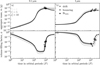 |
Fig. 1 Aggregate mass and volume-filling factor vs time. The heliocentric distance is 30 au. Panels a and b: mass evolution for 0.1 μm and 1 μm sized monomers, while panels c and d: volume-filling factor evolution. The diamond and the circle indicate when the system becomes drift limited and bouncing dominated, respectively. A square indicates when the aggregates reach Stmin = 1.5 × 10⁻³ (Yang et al. 2017). To clearly indicate the case when the system becomes drift limited, the lines continue as dashed lines after this point. |
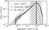 |
Fig. 3 Mass distribution function for 1 μm monomers in the nominal case. Same as Fig. 2, but for 1 μm sized monomers. Here, the mdf differ significantly between drift and bouncing. Growth of aggregates is drift limited, which prevents the aggregates from growing locally to Stmin. |
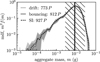 |
Fig. 2 Mass distribution function for 0.1 μm monomers in the nominal case. Mass distribution functions at times when the system becomes drift limited (drift), bouncing dominated (bouncing), and when the aggregates reach Stmin (SI) are plotted. Numbers next to the labels show the times in orbital periods. Vertical lines mark the peak of the distribution function, and the hatched area highlights the region around the peak that contributes 95% to the peak. The mdf show that the system becomes bouncing dominated for 0.1 μm sized monomers. The peak between drift and bouncing changes by ≲ 2%, and the two mdf differ by ≲ 5% around the peak where most of the mass is contained. The larger uncertainties at the low-mass and high-mass ends of the mdf are due to the low resolution of the representative particle method in this part. |
3.2 Parameter study for aggregate growth
We now discuss the influence in more detail that certain parameters and model designs have on aggregate growth. An overview of the variations is given in Table 2, and the results are summarised in Table 3.
Overview of model designs used in parameter study.
Aggregate growth for different model settings.
3.2.1 Heliocentric distance
In addition to the nominal case at 30 au, we performed simulations at 5 au, 15 au, and 50 au to sample the region where comets form.
We find that in the sub-micron case, aggregate growth is bouncing dominated, and we conclude that it is possible for aggregates to reach Stmin allowing for local formation of comets inside ~ 50 au. The picture changes for 1 μm sized monomers. Aggregate growth is bouncing dominated only at 5 au, while it is drift limited for larger heliocentric distances. This means that local formation of comets by streaming instability is not possible in these cases. The maximum mass that can locally be reached decreases from ~ 0.1 g at 5 au to ~ 10−4 g at 50 au (Fig. 4).
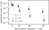 |
Fig. 4 Aggregate mass vs heliocentric distance. Small and large symbols are for 0.1 μm and 1 μm monomers, respectively. A filled square shows the mass of the aggregates that reached Stmin. If Stmin is not reached, the maximum mass to which aggregates can locally grow because of drift (diamond) or bouncing (circle) is shown with an open symbol instead. |
3.2.2 Turbulence
Figure 5 shows that a higher value for the turbulent strength α leads to significantly less porous (before the bouncing barrier) and less massive aggregates, whereas for a lower value of α, we observe the opposite. Furthermore, for higher α, aggregate growth is faster than for lower values of α. The reason for these effects is that the collision velocities are driven by turbulence scale as  . Thus, higher values of α lead to higher velocities, which shifts the onset of bouncing or fragmentation to lower masses and also increases the collision rates, so that coagulation proceeds faster.
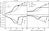 |
Fig. 5 Aggregate mass and volume-filling factor vs time for different values of α. The heliocentric distance is 30 au. Panels a and b: mass evolution for 0.1 μm and 1 μm sized monomers, while panels c and d: volume-filling factor evolution. The diamond and the circle indicate when the system becomes drift limited and bouncing dominated, respectively. A square indicates when the aggregates reach Stmin = 1.5 × 10⁻³ (Yang et al. 2017). To clearly indicate the case when the system becomes drift limited, the lines continue as dashed lines after this point. Increasing or reducing turbulence affects both the mass of the aggregates and the collision rate, i.e. growth is faster for higher values of α. |
3.2.3 Varying the gas surface density
Figure 6 shows that increasing the gas surface density to twice the MMSN value increases the mass of the aggregates, while decreasing the surface density reduces the mass. A higher gas surface density (but fixed metallicity) leads to a lower Stokes number of the aggregates because  . A lower Stokes number, in turn, leads to lower collision velocities, which shifts bouncing and fragmentation to higher aggregate masses. The collision rate, on the other hand, is not affected by varying the gas surface density because in the turbulence-dominated regime, the collision rate is constant and ∝ ZΩ.
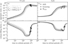 |
Fig. 6 Aggregate mass and volume-filling factor vs time for different disk surface densities. The heliocentric distance is 30 au. Panels a and b: mass evolution for 0.1 μm and 1 μm sized monomers, while panels c and d: volume-filling factor evolution. The diamond and the circle indicate when the system becomes drift limited and bouncing dominated, respectively. A square indicates when the aggregates reach Stmin = 1.5 × 10⁻³ (Yang et al. 2017). To clearly indicate the case when the system becomes drift limited, the lines continue as dashed lines after this point. An increased gas surface density leads to higher aggregate masses, and vice versa. |
3.2.4 Gas-disk dispersal
From observations we know that protoplanetary disks disperse over time with a mean lifetime of τ ≈ 3 Myr (Haisch et al. 2001; Fedele et al. 2010). To test whether the dispersal of the solar nebula gas affects the growth of aggregates, we performed a simulation in which we decreased the gas density exponentially with time as 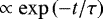 with τ = 3 Myr. Because the effect of a solar nebula dispersal becomes more pronounced with increasing time, we integrated the system for 10 000 orbits insteadof 5000 orbits.
Figure 7 shows the results of this experiment. In the sub-micron case, fragmentation of aggregates is stronger, leading to smaller aggregates at the end of the simulation. The reason for this is the significantly reduced gas density at later times. The reduced friction between gas and aggregates leads to higher Stokes numbers. Thus, the aggregates start to fragment once they traverse the bouncing regime and reach the fragmentation regime. Other than this, aggregate growth is not affected by disk dispersal.
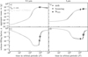 |
Fig. 7 Aggregate mass and volume-filling factor vs time for a dispersing solar nebula. The heliocentric distance is 30 au. Panels a and b: mass evolution for 0.1 μm and 1 μm sized monomers, while panels c and d: volume-filling factor evolution. The diamond and the circle indicate when the system becomes drift limited and bouncing dominated, respectively. A square indicates when the aggregates reach Stmin = 1.5 × 10⁻³ (Yang et al. 2017). To clearly indicate the case when the system becomes drift limited, the lines continue as dashed lines after this point. The solar nebula disperses with mean lifetime of 3 Myr. Reducing the gas density pushes aggregates through the bouncing regime until they start to fragment. Other than this, aggregate growth is not affected. |
3.2.5 Increased stickiness
We tested theeffect of increased stickiness of ice on aggregate growth by increasing the rolling energy and the threshold velocities for sticking, bouncing, and fragmentation of ice by a factor of 5 each.
Stickier ice does not significantly change aggregate growth (see Fig. 8). The aggregates gain at most a factor two in mass. However, increased stickiness prevents aggregate fragmentation towards the end of the simulation.
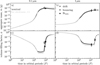 |
Fig. 8 Aggregate mass and volume-filling factor vs time for increased stickiness of ice. The heliocentric distance is 30 au. Panels a and b: mass evolution for 0.1 μm and 1 μm sized monomers, while panels c and d: volume-filling factor evolution. The diamond and the circle indicate when the system becomes drift limited and bouncing dominated, respectively. A square indicates when the aggregates reach Stmin = 1.5 × 10⁻³ (Yang et al. 2017). To clearly indicate the case when the system becomes drift limited, the lines continue as dashed lines after this point. Increasing the threshold velocities of sticking, bouncing, and fragmentation of ice by a factor of 5 does not affect aggregate growth significantly. |
3.2.6 Bouncing only for compact aggregates
We set up a simulation in which we permitted bouncing collisions to occur only for aggregates with volume-filling factors ϕ > 0.1.
The results are shown in Fig. 9. This modification prevents bouncing collisions because collisional compression in sticking collisions increases the volume-filling factors of the aggregates only to ϕ = 10−4 to 10−2 depending onmonomer size. The aggregates then start to fragment until a growth/fragmentation equilibrium is reached. Fragmentation increases the volume-filling factor, because we kept the fractal dimension constant (and not the volume-filling factor; see Appendix B.4.3), which implies that the fragments have a higher volume-filling factor than the progenitor aggregate. At the end, the volume-filling factors of the bulk of the aggregates are 10−3 and 10−2 for the sub-micron and micron cases, respectively.
Without the bouncing barrier, aggregates grow to much larger sizes before fragmentation sets in. Because of the high porosityof the aggregates, the growth timescale is shorter than radial drift and the maximum mass of the aggregates is limited by fragmentation. Aggregates grow to Stmin regardless of initial monomer size.
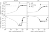 |
Fig. 9 Aggregate mass and volume-filling factor vs time for the case of limited bouncing. The heliocentric distance is 30 au. Panels a and b: mass evolution for 0.1 μm and 1 μm sized monomers, while panels c and d: volume-filling factor evolution. The diamond and the circle indicate when the system becomes drift limited and bouncing dominated, respectively. A square indicates when the aggregates reach Stmin = 1.5 × 10⁻³ (Yang et al. 2017). To clearly indicate the case when the system becomes drift limited, the lines continue as dashed lines after this point. Only aggregates with volume-filling factor ϕ ≥ 0.1 are allowed to bounce. While aggregates generally grow to higher masses, their volume-filling factors remain very low, and bouncing collisions practically do not occur. In both cases, Stmin is reached. |
4 Discussion
4.1 Implications for comet formation
We found in Sect. 3.1 that depending on the monomer size, the system evolves differently because of porosity effects. While aggregate growth is drift limited for 1 μm sized monomers, which prevents growth up to Stmin, aggregate growth is bouncing dominated for 0.1 μm sized monomers. The latter case allows aggregates to reach Stmin through collisional compression in bouncing collisions. Because the compression is faster than the radial drift of the bouncing aggregates, streaming instability leading to local formation of comets should be possible. The aggregates that would participate in the streaming instability have masses between 0.1 mg and 100 mg and volume-filling factors between 10−2 and 0.1.
Varying different parameters in our simulations affects aggregate growth differently, as shown in the previous section. However, our result that growth from 1 μm sized monomers is drift limited, which prevents aggregates from reaching Stmin, is seen throughout the parameter study. The same holds for our result for 0.1 μm sized monomers, which evolve into a bouncing-dominated system of aggregates.
Poulet et al. (2016) measured the sizes of pebbles on comet 67P, which they argued cannot have formed recently because their size distribution differs significantly from young cometary particles (dust in the coma, boulders on the surface). The measured pebbles are most likely the building blocks from which the comet once formed, although a different formation process, for example, through erosive processes or redeposition (Bibring et al. 2015), cannot be entirely ruled out (Poulet et al. 2016). Pebble sizes are in the range 3 mm to 1.6 cm. Towards small pebble sizes (<5 mm), the cumulative size-frequency distribution of the pebbles reaches a plateau, which is partly attributed to the spatial resolution of ~ 1 mm of the CIVA images (Poulet et al. 2016).
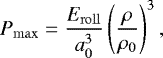
In Figs. 10 and 11, we compare our results to the 3 mm to 1.6 cm size range of 67P pebbles. Because we find in our simulations that the aggregates are porous when reaching Stmin, we need to take compression of aggregates during the gravitational collapse of the pebble-cloud into account to obtain a comet-like planetesimal (Lorek et al. 2016). This compression requires pebble clouds with masses equivalent to planetesimals ≳100 km, which is also the typical size found in numerical simulations of planetesimal formation by streaming instability (Johansen et al. 2007; Schäfer et al. 2017).
From Table 2 and Fig. 4 of Lorek et al. (2016), we can estimate the maximum volume-filling factor, ϕmax, to which aggregates are compressed during the collapse, depending on cloud mass, initial volume-filling factor, and dust-to-ice ratio. For a pebble-cloud with a mass equivalent to a 100 km planetesimal, ϕmax is in the range between 0.24 and 0.37 for dust dust-to-ice ratios between 1 and 10, respectively. We calculated the post-collapse radius, a*, of the aggregates from the definition of the volume-filling factor as 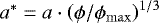 and applied it to the aggregates from our simulations. We then compared these radii to the size range of 67P pebbles.
We find that the post-collapse aggregate radii are in broad agreement with what is found on 67P if the comet forms in situ at a distance between 5 au and 15 au (see Fig. 10). However, at our nominal location at 30 au and beyond, the post-collapse radii of the aggregates are with typically 1 mm slightly smaller than the observed pebbles on 67P, unless the dust-to-ice ratio is unity. However, if all aggregates had a dust-to-ice ratio of unity, it would imply that the comet had a dust-to-ice ratio of unity, which is neither in agreement with measurements (dust-to-ice ratio ~4–6 Rotundi et al. 2015; Fulle 2017) nor with models of comet formation in collapsing pebble-clouds (dust-to-ice ratio ~3–9 Lorek et al. 2016).
A less turbulent environment promotes the growth of larger aggregates because lower collision velocities prevent aggregates from fragmentation. The post-collapse radii of these aggregates agree very well with the measured size range of pebbles on 67P.
Limiting bouncing collisions to compact aggregates only produces larger aggregates. While the post-collapse aggregate radius is within the observed range for 1 μm sized monomers, they are twice as large as the largest pebbles on 67P for 0.1 μm sized monomers. Bentley et al. (2016) measured the sub-structure of dust aggregates from 67P with the atomic force microscope of the MIDAS experiment on board Rosetta. They found that even the aggregates of about 1 μm in size consist of smaller units down to 0.1 μm. Even smaller units cannot be excluded because of the resolution limit of the MIDAS experiment. We conclude from this that without bouncing collisions, aggregates would most likely be larger than the observed pebble sizes for a realistic range of the monomer size between sub-micrometre and micrometre.
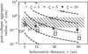 |
Fig. 10 Post-collapse aggregate radius vs heliocentric distance. The hatched area marks the range of pebble sizes measured on 67 P by the CIVA camera on board Rosetta/Philae (Poulet et al. 2016). The square symbols show aggregate sizes at Stmin. Large and small symbols are for 1 μm and 0.1 μm sized monomers, respectively. Symbols are filled if aggregates might trigger the streaming instability (Table 3). Dashed lines indicate the minimum size for aggregates with a given volume-filling factor to have Stmin. ϕ0 refers to the initial aggregate porosity (i.e. before compression). |
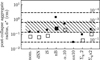 |
Fig. 11 Post-collapse aggregate radii for the parameter study at 30 au. Symbols, hatched area, and dashed curves are the same as in Fig. 10. The abbreviations for the different models are the same as in Table 2. |
4.2 Comparison with dust coagulation models
Krijt et al. (2015) investigated coagulation of icy dust including a simple erosion model. Erosion of the target occurs when the mass ratio between projectile and target is low and the collision speed is higher than an erosion threshold velocity. The threshold is taken between 20 m s−1 (efficient erosion) and 60 m s−1 (inefficient erosion). For efficient erosion, Krijt et al. (2015) found that aggregates grow to a maximum mass of ~109 g (see their Fig. 13) with Stokes numbers suitable for streaming instability. Their highly porous aggregates would be several tens of metres in the comet-forming region (see Fig. 14 of Krijt et al. 2015). Even compressed, the aggregates would have sizes of a few metres, which is orders of magnitudes larger than what is observed by CIVA (Poulet et al. 2016). However, the so-called goosebumps have characteristic sizes of a few metres (Sierks et al. 2015; Davidsson et al. 2016). Whether the goosebumps are pristine structures is still under debate.
Krijt et al. (2016) modelled coagulation of icy dust in the entire disk. They found that while erosion-limited growth of icy aggregates can easily produce aggregates with the right Stokes number for streaming instability, the mass loading in the disk midplane is too low in large parts of the disk. Estrada et al. (2016) performed global simulations of dust growth in protoplanetary disks. While they took detailed physics into account, such as condensation fronts and a collision model comparable to ours, porosity was not considered. They found that with low turbulence (α = 4 × 10⁻⁴), aggregates grow to sizes in the range 10−2 cm to 10 cm in the comet-forming region between 5 au and 50 au. For stronger turbulence (α = 4 × 10⁻³), aggregates reach sizes in the range between 0.1 cm to 1 cm (see their Fig. 17). In both cases, the Stokes numbers are around 10−2, which, according to Yang et al. (2017), should be high enough for streaming instability. However, they also found that the mass loading in the midplane is typically too low (well below unity, with one exception, close to evaporation front around 5 au).
Compared to Krijt et al. (2015, 2016), our aggregates have masses orders of magnitude lower. This is expected because bouncing terminates growth at masses ≲10−1 g in the collision model used in our study. On the other hand, erosion sets in when the collision velocity between two aggregates with a mass ratio below a critical value of 10−2 exceeds the erosion threshold in the collision model used by Krijt et al. (2015). Aggregates need to grow to St ~ 1 to develop significant collision speeds as a result of differential radial drift. This terminates growth at masses of ≳104–108 g depending on porosity. The aggregates in Estrada et al. (2016) have a density of roughly 1.5 g cm−3. Thus, masses are between 6 mg and 6 g in the strong turbulence case. This compares reasonably well to our results because the collision model used in Estrada et al. (2016) is similar to the one used here, although without porosity. However, we also find that the mass loading in the midplane is too low.
Lastly, Zsom et al. (2010) and Windmark et al. (2012) found a bouncing-dominated population of dust aggregates. Their simulations were located at 1 au and 3 au, respectively, which is inside the region relevant for comet formation. However, their results, that is, that bouncing produces a narrow size distribution of aggregates, compare well with our findings.
4.3 Caveat: dust concentration
The main focus of our study was on the question whether aggregates reacha minimum size, respectively Stokes number, for streaming instability to be possible. We omit the problem of aggregate concentration such that the local mass loading exceeds unity. However, a mass loading ≳1 is an important prerequisite for the streaming instability. The sedimentation of aggregates to the disk midplane, which is the only process about which we can make a statement, is not sufficient to produce this condition because the mass loading remains low,  for typical values of Z = 0.03, α = 10−3, and St = Stmin ≈ 10−3 (see also Krijt et al. 2016; Estrada et al. 2016). Hence, there is a formidable gap between our simulation results, showing that aggregates would have the right aerodynamic properties and the actual onset of the streaming instability. However, we speculate that under realistic conditions in a turbulent disk, a concentration of aggregates in pressure maxima between turbulent eddies that have overturn timescales of the order of the stopping time of Stmin aggregates (e.g. Cuzzi et al. 2001, 2010; Cuzzi & Weidenschilling 2006) or pile-up of material caused by pressure bumps or vortices should be possible (e.g. Kretke & Lin 2007; Johansen et al. 2009; Pinilla et al. 2012). We leave a more quantitative assessment for future work and only stress that this problem clearly is a caveat of our study.
4.4 Caveat: local approximation
The local approximation (tgrow ≲ tdrift, Sect. 3) we made use of in our simulations holds true if the total drift distance of the aggregates Δrdrift = ∫ Δvr dt is small compared to the orbital distance (Δrdrift ≪ r) (Ormel et al. 2008). Here, Δvr is the radial drift velocity of aggregates (Eq. (A.7)). Integrating from time t = 0 (start of the simulation) until the time when aggregates become bouncing dominated, Δrdrift∕r ≈ 10−3 for 0.1 μm sized monomers at 30 au, whereas Δrdrift∕r ≈ 10−1 for 1 μm sized monomers. Hence, the local approximation is fine for sub-micrometre monomers. However, for larger monomers, aggregates drift ≈10% closer to the Sun, which corresponds to a few astronomical units at 30 au and might already affect the growth process. Calculating Δrdrift for the time interval from the bouncing barrier until aggregates reach Stmin due to compression (ΔtSt) gives similar values of Δrdrift∕r ≈ 10−2 for 0.1 μm sized monomers. Hence, we conclude that the local approximation is valid for 0.1 μm sized monomers and that aggregates can locally reach the right aerodynamic properties for streaming instability.
4.5 Caveat: collision model
As there were most likely no pure dust and ice aggregates present in the solar nebula, we used aggregates of mixed composition and implemented a collision model, which interpolates linearly between the collision properties of pure ice and pure dust aggregates (see Appendix B.5). However, there are limitations to this approach. Although we have detailed knowledge about dust from laboratory experiments (e.g. Güttler et al. 2010; Windmark et al. 2012), data for ice aggregates are sparse, but they support the key idea of scaling the threshold quantities for ice by a factor of ten (e.g Gundlach et al. 2011a; Gundlach & Blum 2015).
The bouncing behaviour of highly porous aggregates is very uncertain. Numerical experiments by Wada et al. (2011); Seizinger & Kley (2013) predict bouncing only for compact aggregates (volume-filling factors ≳0.3). On the other hand, bouncing was observed for aggregates with volume-filling factors ≳0.1 (Güttler et al. 2009; Weidling et al. 2009) and recently also for aggregates with volume-filling factors of 0.15 and coordination numbers of 2, comparable to highly porous and fractal aggregates (Landeck 2016). The experiments by Landeck (2016) are in contrast to the numerical results, which require coordination numbers ≳6 for bouncing.We emphasise that our collision model does not predict bouncing for fractal aggregates, which has indeed never been observed. The formation of fractal aggregates is associated with hit-and-stick collisions (ballistic cluster-cluster aggregation) without internal restructuring of the aggregates. When the collision energy increases and eventually exceeds the rolling energy of the monomers, sticking collisions result in restructuring and compression. This ends fractal growth because the internal structure becomes more homogeneous with each collision. Thus, bouncing aggregates might be highly porous with a coordination number of 2, but not fractals. This is in agreement with the Landeck (2016) results. As we rely on experimental work for our collision model, this is a key argument for including bouncing. However, our implementation of bouncing for porous aggregates should be considered as a hypothesis which needs to be explored in the future with more laboratory experiments and with numerical simulations of aggregate collisions.
5 Summary
We studied the growth of aggregates from a two-component system of (sub-)micrometre-sized dust and ice monomers to find the properties of aggregates that trigger the streaming instability and become the building blocks of comets formed by gravitational collapse of pebble-clouds. We used aggregates of mixed composition and implemented a collision model for these aggregates based on interpolating the collision behaviour between pure ice and pure dust aggregates (Lorek et al. 2016); we also included porosity. The dust-to-ice ratio in our simulations were in the range between 1 and 10. With these tools, we performed Monte Carlo simulations of coagulation, employing the representative particle approach developed by Zsom & Dullemond (2008). We used the measurements of pebbles on 67P (Poulet et al. 2016) to discuss the implication of our aggregate growth model for comet formation. Our main findings are listed below.
In general, aggregate growth is bouncing dominated for 0.1 μm sized monomers and drift limited for 1 μm sized monomers. In the bouncing-dominated cases, aggregates reach Stmin as a result of compression in bouncing collision before the bouncing aggregates are removed by radial drift. In the drift-limited cases, aggregates do not reach Stmin.
Because of the low value of Stmin, aggregates that would participate in the streaming instability in the comet-forming region around 30 au are porous, with volume-filling factors ~10−2, but more compact (volume-filling factor ~0.1) closer to the Sun; their sizes are of a few millimetres. However, these are the properties of aggregates before the pebble-cloud collapse. Taking compression during the collapse into account, we obtained post-collapse aggregate radii that broadly agree with the pebbles measured on comet 67P (Poulet et al. 2016).
Our result, that is, that aggregates are porous when triggering the streaming instability, requires comet formation in pebble-clouds with masses equivalent to planetesimals ≳100 km in diameter (Lorek et al. 2016). This would be in agreement with the typical mass of pebble-clouds that formed in numerical simulations of a streaming instability (Schäfer et al. 2017).
Acknowledgements
The authors thank the referee for constructive feedback and a discussion that helped improving the quality of this manuscript. S. Lorek is a member of the International Max Planck Research School (IMPRS) for Solar System Science at the Max Planck Institute for Solar System Research (MPS) in Göttingen.
Appendix A Gas disk model
A.1 Disk structure
In the MMSN, the gas surface density and the gas temperature decrease with heliocentric distance (r) according to 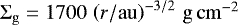 and
and 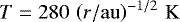 , respectively (Weidenschilling 1977b; Hayashi 1981). The mean molecular weight of the gas is μ = 2.34, which results in a sound speed of
 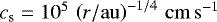 . The mean thermal velocity of the gas molecules is
  . The Keplerian orbital frequency is
  , and the Keplerian velocity is vK = r Ω. Thus, we obtain for the relative pressure scale height of the gas disk
  . The disk is in hydrostatic equilibrium, which results in a Gaussian vertical density profile
  , where z is the height above the midplane.
The dust distribution follows the gas distribution, which means that the density profile of the dust is also Gaussian,
 (A.1)
(A.1)
where Σd = Z Σg is the dust surface density, and Z is the metallicity (solid-to-gas ratio). The nominal value for the metallicity is Z = 1% (Dubrulle et al. 1995; Carballido et al. 2006). The scale height of the dust is
![Mathematical equation: \begin{equation} h_\mathrm{d}=h_\mathrm{g}\left[1+\frac{\stokes}{\alpha}\frac{1+2\stokes}{1+\stokes}\right]^{-1/2} \label{eq:dustscaleheight} \end{equation}](/articles/aa/full_html/2018/03/aa30175-16/aa30175-16-eq18.png) (A.2)
(A.2)
(Dubrulle et al. 1995; Carballido et al. 2006; Youdin & Lithwick 2007) and depends on the disk turbulence via the α-parameter (Shakura & Sunyaev 1973) and the coupling of solids to gas characterised by the Stokes number St (see Appendix A.2). Aggregates start to settle towards the midplane once they reach Stokes numbers St ≫ α.
A.2 Drag force
In contrast to the dust aggregates, the solar nebula gas is pressure supported and orbits at sub-Keplerian speed,  , where η is related to the pressure gradient (Weidenschilling 1977a; Nakagawa et al. 1986)
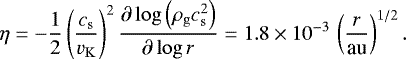 (A.3)
(A.3)
The dust aggregates experience a drag force fD = 1∕2 CDAρgΔv2, where CD is the drag coefficient, A is the geometrical cross-section of the aggregate, and Δv is the relative velocity between dust and gas. The drag coefficient takes different values depending on the ratio of aggregate size (a) and mean free path (λ) of the gas molecules and the Reynolds number (Re) of the gas flow around the aggregate. The mean free path is λ = μmH∕ρgAmol, where Amol = 2 × 10⁻¹⁵ cm2 is the collisional cross-section of the gas molecules. The Reynolds number is Re = 2aΔv∕ν, where ν = 1∕2 λvthm is the molecular viscosity.
Following Weidenschilling (1977a), the drag coefficient is
 (A.4)
(A.4)
in the Epstein regime for λ∕a > 4∕9, and takes values
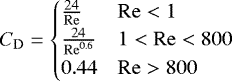 (A.5)
(A.5)
in the Stokes and non-linear regimes, where λ∕a < 4∕9.
We used the drag force to define the stopping time of the aggregates as ts = mΔv∕fD. From the stopping time, we constructed the dimensionless Stokes number as St = Ωts. The Stokes number quantifies the coupling between the dust aggregates and the gas. For St ≪ 1, the dust aggregates are very well coupled to the gas and follow the gas flow, while for St ≫ 1, dust and gas are decoupled and the dust aggregates are exposed to a constant headwind, ηvK, which causes them to slowly spiral towards the Sun. For St ≈ 1, dust and gas are marginally coupled.
We considered three sources of relative velocities between gas and dust: turbulent stirring, radial drift, and azimuthal drift. Brownian motion is, in principle, also a source of relative velocity between gas and dust. We neglected it here and included Brownian motion only for relative velocities between aggregates (see Appendix B.2). Turbulent stirring is caused by the turbulent motion of the gas. According to Cuzzi & Hogan (2003); Ormel & Cuzzi (2007), we have
 (A.6)
(A.6)
where Ret = αcshg∕ν is the turbulent Reynolds number.
Radial and azimuthal drift are both a consequence of the sub-Keplerian motion of the gas due to the pressure support and the headwind on the dust aggregates. The radial drift velocity is
 (A.7)
(A.7)
and the azimuthal drift relative to Keplerian speed is
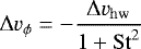 (A.8)
(A.8)
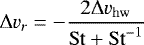
(Weidenschilling 1977a). Here, Δvhw is the disk headwind velocity, which is the velocity difference between the gas velocity and Keplerian speed, Δvhw = vK − vg = η vK. For the azimuthal drift of the dust relative to the gas, we then have to take  . To obtain the total relative velocity between gas and dust, we summed the squares of the individual components and took the square root
 (A.9)
(A.9)
We used Δv to calculate the Stokes number of the aggregates.
In the Epstein regime and the first Stokes regime, we can easily calculate the Stokes number as St does not depend on Δv. For Re > 1, however, the Stokes number depends on the relative velocity between gas and dust through the drag coefficient, and the relative velocity depends on the Stokes number. In this case, we used an iterative scheme to self-consistently determine Δv and St.
Appendix B Dust collision model
To study the growth of aggregates of mixed composition through coagulation from a two-component system of dust and ice monomers, we employed the collision model outlined in Lorek et al. (2016).
B.1 Dust properties
B.1.1 Monomers
We used (sub-)micrometre-sized monomers, which are composed of either silicate dust or water ice, and required that all monomers have the same size. The bulk densities of the dust and water ice monomers were ρd = 3 g cm−3 and ρi = 1 g cm−3, respectively. The rolling friction force was measured in the laboratory for a0 = 1.45 μm ice monomers and is Froll = 114.8 × 10⁻⁵ dyn, while Froll = 12.1 × 10⁻⁵ dyn for a0 = 0.75 μm SiO2 monomers (Gundlach et al. 2011a). The rolling friction force is important for modelling the porosity evolution of the aggregates. According to Krijt et al. (2014), the rolling friction force scales with monomer radius as  . The rolling energies for dust and ice are then
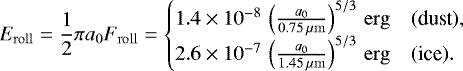 (B.1)
(B.1)
Compared to dust, the rolling energy of ice is roughly ten times higher. Thus, we can already expect that aggregates with a higher dust content are easier to compress.
B.1.2 Aggregates
The aggregates are agglomerates of Nd dust and Ni ice monomers. Mass and volume-filling factor describe the aggregates, from which other properties, such as size and density, can be derived. The volume-filling factor is defined as the ratio of compact volume to actual volume as ϕ = NV0∕V, where N = Nd + Ni is the total number of monomers, V0 is the volume of a single monomer, and V is the aggregate volume. The aggregate volume is V = 4πa3∕3, where a is the characteristic radius of the aggregate (Okuzumi et al. 2009).
The volume-filling factor is a measure for the porosity of the aggregate, as it quantifies the amount of void space within the aggregate. A volume-filling factor of ϕ = 1 describes a solid sphere with no void space, while ϕ = 0.1 corresponds to an aggregate with 90% porosity. Therefore, monomers have ϕ = 1, but the aggregates will have ϕ < 1, in general.
For the aggregate-gas interaction (see Appendix A.2), the geometrical cross-section of the aggregate is relevant. We calculated the geometrical cross-section according to Eq. (47) of Okuzumi et al. (2009). The collisional cross-section, relevant for collisions between two aggregates, is given by π(a1 + a2)2.
B.2 Collision velocities
Collisions between aggregates are driven by Brownian motion, turbulence, and radial and azimuthal drift. We restrict our study to the disk midplane, which means that the vertical settling velocity is zero.
The relative velocity between two aggregates of masses m1 and m2 due to Brownian motion is
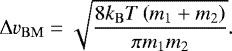 (B.2)
(B.2)
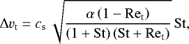
For turbulence induced collisions, we used the closed form expressions given in Ormel & Cuzzi (2007) for St2 ≤ St1
![Mathematical equation: \begin{align} &{\rm{\Delta}} v_\mathrm{t}^2=\alpha c_\mathrm{s}^2 \nonumber \\* &\times\begin{cases} \frac{\stokes_1-\stokes_2}{\stokes_1+\stokes_2}\left(\frac{{\stokes_1^2}}{{\stokes_1+\mathrm{Re}_\mathrm{t}^{-1/2}}}-\frac{{\stokes_2^2}}{{\stokes_2+\mathrm{Re}_\mathrm{t}^{-1/2}}}\right) & \stokes_1,\stokes_2<\mathrm{Re}_\mathrm{t}^{-1/2} \\ \left[2y_\mathrm{a}-\left(1+\beta\right)+\frac{2}{1+\beta}\left(\frac{1}{1+y_\mathrm{a}}+\frac{\beta^3}{y_\mathrm{a}+\beta}\right)\right]\stokes_1 & \mathrm{Re}_\mathrm{t}^{-1/2}<\stokes_1<1 \\ \frac{1}{1+\stokes_1}+\frac{1}{1+\stokes_2} & \stokes_1>1 \end{cases}, \end{align}](/articles/aa/full_html/2018/03/aa30175-16/aa30175-16-eq31.png) (B.3)
(B.3)
where ya = 1.6 and β = St1∕St2.
The relative velocities introduced by differential drift follow from Eqs. (A.7) and (A.8) as
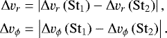 (B.4) (B.5)
We summed the squares of the individual contributions to obtain the total collision velocity between aggregates 1 and 2,
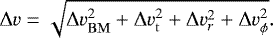 (B.6)
(B.6)
The collision energy,
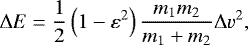 (B.7)
(B.7)
is the amount of energy that is dissipated within the aggregate in the collision and is therefore available for restructuring and breaking bonds between the monomers. Here, ε is the coefficient of restitution. For purely inelastic collision, as is the case for sticking, ε = 0; while for purely elastic collision ε = 1. Otherwise, when collisions lead to bouncing but dissipate energy, the coefficient of restitution is in the range 0 < ε < 1.
B.3 Collision regimes
From laboratory work (e.g. Güttler et al. 2010), we know that collisions between dust aggregates lead to various outcomes. These are sticking, bouncing, fragmentation, erosion, and mass transfer, depending on the collision velocity Δv (Windmark et al. 2012).
Windmark et al. (2012) provided the threshold velocities forsticking, bouncing, and the onset of fragmentation of dust aggregates as power laws in mass, Δv ∝ mb, with a slope b = −5∕18 for sticking and bouncing collisions
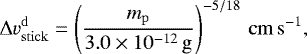 (B.8)
(B.8)
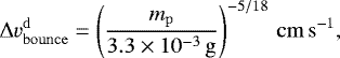 (B.9)
(B.9)
and b = −0.16 for fragmentation
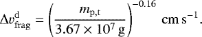 (B.10)
In each case, the normalisation constants were obtained from laboratory experiments (see Weidling et al. 2012, for details). Here, mp,t is the mass of projectile or target, respectively. In the case of fragmentation, the threshold velocity is compared to the centre-of-mass velocity of target and projectile,
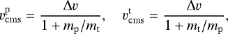 (B.11)
in order to calculate fragmentation of target and projectile individually, which is important for the distinction between global fragmentation of both aggregates, mass transfer, and erosion.
The threshold velocities Eqs. (B.8)–(B.10) are valid for dust aggregates. For ice, we scaled the threshold velocities by factor of 10, for instance,  , and similar for bouncing and fragmentation, as laboratory work by Gundlach & Blum (2015) suggests.
B.4 Porosity
Porosity evolution is a key component in our simulations. Here, we summarise how sticking, bouncing, fragmentation, and non-collisional processes change the porosity of the aggregate.
B.4.1 Sticking collisions
We included the Okuzumi et al. (2012) porosity model for sticking collisions. Equations (B.12)–(B.14) of this model describe the whole bandwidth from hit-and-stick collisions without restructuring, which produce fractal aggregates, to sticking collisions with compression. For two dust aggregates of volumes V1 and  , a sticking collision results in an aggregate with a new volume of
![Mathematical equation: \begin{equation} V_{1+2}=\left[\left(1-\frac{{\rm{\Delta}} E}{3bE_\mathrm{roll}}\right)V_{1+2,\,\mathrm{HS}}^{5/6}+\frac{{\rm{\Delta}} E}{3bE_\mathrm{roll}}\left(V_1^{5/6}+V_2^{5/6}\right)\right]^{6/5}, \label{eq:newvolume1} \end{equation}](/articles/aa/full_html/2018/03/aa30175-16/aa30175-16-eq41.png) (B.12) if
(B.12) if  and ΔE < 3bEroll,
![Mathematical equation: \begin{equation} V_{1+2}=\left[\frac{\left(3/5\right)^5\left({\rm{\Delta}} E-3bE_\mathrm{roll}\right)}{N_{1+2}^5bE_\mathrm{roll}V_0^{10/3}}+\left(V_1^{5/6}+V_2^{5/6}\right)^{-4}\right]^{-3/10}, \label{eq:newvolume2} \end{equation}](/articles/aa/full_html/2018/03/aa30175-16/aa30175-16-eq43.png) (B.13)
(B.13)
if  and ΔE > 3bEroll, or
![Mathematical equation: \begin{equation} V_{1+2}=\left[\frac{\left(3/5\right)^5{\rm{\Delta}} E}{N_{1+2}^5bE_\mathrm{roll}V_0^{10/3}}+V_{1+2,\mathrm{HS}}^{-10/3}\right]^{-3/10}, \label{eq:newvolume3} \end{equation}](/articles/aa/full_html/2018/03/aa30175-16/aa30175-16-eq45.png) (B.14)
(B.14)
if  . Here, b = 0.15 is a fitting parameter from the numerical work of Wada et al. (2008). V0 is the volume of a single monomer, N1+2 = (m1 + m2)∕m0 is the number of monomers in the new aggregate, and m0 is the monomer mass. Finally, V1+2, HS = V1 + V2 + Vvoid is the volume of the new aggregate for a hit-and-stick collision, where Vvoid is the void space created in the collision,
 (B.15)
The coefficient of restitution in Eq. (B.7) used in Eqs. (B.12)–(B.14) is set to ε = 0 because the aggregates stick to each other.
B.4.2 Bouncing collisions
Bouncing collisions compress the aggregates. We used the compression curves of dust and ice aggregates to calculate the change in volume-filling factor in a single collision (Güttler et al. 2010; Lorek et al. 2016). The aggregate is compressed if ϕ < ϕmax, where ϕmax is the maximum volume-filling factor according to the compression curve and ϕ is the current value of the aggregate. The functional form of the compression curve is given by
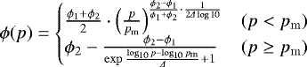 (B.16)
(Güttler et al. 2009, 2010). Here, p is the pressure applied to the aggregate in the collision. The pressure depends on aggregate density, ρ, and collision velocity, Δv, as p ∝ ρΔv2. For the parameters ϕ1, ϕ2, Δ, and pm, we summarise the values in Table B.1.
Parameters for the dust and ice compression curves.
B.4.3 Fragmentation, mass transfer, and erosion
We followed Krijt et al. (2015) and assumed that the fragments produced in a fragmenting or erosive collision have the same fractal dimension, Df, as the progenitor aggregate. We estimated the fractal dimension according to
![Mathematical equation: \begin{equation} D_\mathrm{f}=3\left[1-\frac{\log_{10}\phi}{\log_{10}N}\right]^{-1}, \label{eq:fractaldimension} \end{equation}](/articles/aa/full_html/2018/03/aa30175-16/aa30175-16-eq49.png) (B.17)
(B.17)
where N is the total number of monomers and ϕ is the volume-filling factor of the target before the collision. We then calculated the new aggregate radius from the general mass-radius relation, m ∝ aDf, for fractal aggregates. Because the volume-filling factor is ϕ = N1−3∕Df, the fragment is more compact than the progenitor aggregate for Df ≲3, which is the case for porous aggregation (see Wada et al. 2008, Df ≈ 2.5). An increase in volume-filling factor furthermore reflects the fact that aggregates should be compressed in energetic fragmenting collisions.
B.4.4 Non-collisional compression
Kataoka et al. (2013a) introduced non-collisional mechanisms that further compress the aggregates. These are compaction due to self-gravity and compaction due to ram-pressure of the gas. We included both self-consistently in our simulations. Based on Kataoka et al. (2013b), the maximum pressure an aggregate of density ρ can withstand is
 (B.18)
where ρ0 is the monomer density. This means that we can calculate the equilibrium density 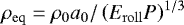 for a given pressure P ≥ Pmax. P is the sum of the gravitational pressure Pgrav = Gm2∕πa4 and the ram pressure of the gas Pram = mΔvΩ∕πa2St. Again, Δv is the relative velocity between gas and dust. The pressure depends on the density of the aggregate because ρ = m∕V and the volume is 4πa3∕3. This requires an iterative scheme to self-consistently calculate ρeq. As the aggregate is compressed, the interaction with the gas changes because the geometrical cross-section changes. Thus, the Stokes number has also to be re-evaluated at each iteration step.
B.5 Mixed aggregates
We adjusted the collision and porosity model for the treatment of a two-component system consisting of dust and ice monomers. As mentioned in Appendix B.1.1, we assumed a single size for the monomers, regardless of composition. We used the fractional abundance of dust monomers, x = Nd∕N, within the aggregate to linearly interpolate the collision behaviour between the cases of pure dust and pure ice (see Lorek et al. 2016, for details).
Thus, we write the threshold velocity for sticking as
 (B.19)
and similar for bouncing and fragmentation.
Accordingly, because it is important for the porosity model, we introduce the rolling energy for mixed aggregates as
 (B.20)
and the compression curve as
 (B.21)
Furthermore, because of our assumption that all monomers have the same size, we can write ρ0 in Eq. (B.18) as 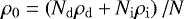 .
.
A final remark on the fractional abundance of dust monomers that we used. When it was necessary to treat target and projectile together, we took  . This is the case for the sticking and bouncing threshold velocities and for the rolling energy in the collisional compression in sticking collisions. In contrast, when the two aggregates were treated individually, we used
  . This is the case for the fragmentation threshold velocity, the compression curve, and the rolling energy in the non-collisional compression.
Appendix C Numerical method
To study the growth from (sub-)micrometre-sized monomers to aggregates, we employed the representative particle approach of Zsom & Dullemond (2008) (see also Ormel et al. 2007; Zsom et al. 2010; Dra̧żkowska et al. 2013, 2014; Dra̧żkowska & Dullemond 2014, for further details).
C.1 Representative particle approach
The representative particle approach is a Monte Carlo method for studying the mass evolution of an ensemble of particles. As it is a particle-based method, additional material properties in addition to the mass, for example, porosity, can easily be added. The ensemble of 𝒩 physical particles has a total mass ℳ. The particles are homogeneously distributed in a volume 𝒱. We chose a number of  particles at random, the so-called representative particles. Each representative particle accounts for a fixed fraction of the total mass, Mswm = M∕n, which means that each representative particle i of mass mi carries along a swarm of 𝒩i = Mswm∕mi identical swarm particles with the same properties as the representative particle. The representative particles are allowed to interact with all other swarm particles (including their own), but not with other representative particles. For this to hold, we require
  for all representative particles. To evolve the system in time, we calculate the collision rate between representative particle i and swarm j for i, j = 1, …, n according to the particle-in-a-box approximation:
 (C.1)
(C.1)
where σij is the collisional cross-section and Δvij is the collision velocity between representative particle i and swarm j. The collision rate between a representative particle i and any swarm particle j is obtained by summing Eq. (C.1) over all swarms j
 (C.2)
(C.2)
and, consequently, the total collision rate by summing Eq. (C.2) over all representative particles i
 (C.3)
(C.3)
Let now t be the current time, the next collision occurs at t + δt, where the time step is calculated from the total collision rate according to  , with u being a random number with uniform distribution in the interval between 0 and 1.
Once we know the time of the next collision, we determine the collision partners. The probability that representative particle i undergoes the collision is Pi = Ci∕C. Thus, interpreting a new random number u as the cumulative probability P≤i = ∑l≤iPl gives the representative particle i as the largest index l for which P≤i > u but l+ 1 would result in P≤i < u. Since we fixed the representative particle, we find the swarm particle in a similar fashion by drawing another random number and comparing it to the probability Pij = Cij∕Ci.
Based on our collision model, we then calculated the collision outcome. However, only the properties of the representative particle i change. The swarm particle j remains unchanged because we only followed the representative particles. In case of sticking, for instance, the mass of representative particle i was updated to mi ← mi + mj.
Finally, we updated the collision rates and repeated the procedure until the final time of our simulation was reached. For details on how to efficiently update the collision rates, see Zsom & Dullemond (2008).
C.2 Vertically integrated collision rate
We performed our simulations in the midplane of a 1D column with surface area 𝒮 located at fixed heliocentric distance r. Thus, we needed to vertically integrate the collision rate, Eq. (C.1), while taking into account that aggregates i and j follow a Gaussian density distribution (see Appendix A.1). This leads to
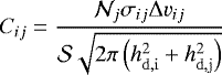 (C.4)
(C.4)
for the final collision rate (Okuzumi et al. 2012; Krijt et al. 2015).
Appendix D Validity check – only sticking collisions
We ran simulations with the simple assumption of perfect sticking for all collisions. This allowed us to compare our results qualitatively to Krijt et al. (2015) and Okuzumi et al. (2012).
The initial conditions were the same as for the simulations discussed in the main text. While aggregate growth was due to porosity faster than radial drift at a heliocentric distance of 5 au, growth was drift limited for larger distances (≳15 au, see Figs. D.1 and D.2), which is in agreement with previous studies (Okuzumi et al. 2012; Kataoka et al. 2013b; Krijt et al. 2015).
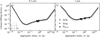 |
Fig. D.1 Volume-filling factor vs peak mass at heliocentric distance of 5 au. Monomer size is a) 0.1 μm, and b) 1 μm. A square indicates when the aggregates reach Stmin (Yang et al. 2017). A triangle pointing to the right denotes the change from the Epstein drag regime to the Stokes drag regime. We plot the results in the same way as Okuzumi et al. (2012). |
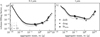 |
Fig. D.2 Volume-filling factor vs peak mass at heliocentric distance of 30 au. Symbols as in Fig. D.1. Additionally, the diamond indicates the drift limit. To clearly indicate the case when the system becomes drift limited, the lines continue as dashed lines after this point. Even though aggregate growth is drift limited and planetesimals cannot form directly, aggregates with Stmin can form. |
Despite growth being drift-limited at 30 au, aggregates still reached the minimum Stokes number (Fig. D.2). In the sub-micron case, the aggregates had masses in the range 430 g and 3700 g and volume-filling factors in the range from 5.2 × 10⁻⁵ to 1.1 × 10⁻⁴. While for 1 μm sized monomers, masses were significantly lower, with values in the range from 0.1 g to 3 g, and the volume-filling factors were higher, with values between 1.7 × 10⁻³ to 6.3 × 10⁻³.
Post-collapse radii of the aggregates were in the ranges 2.5–6.2 cm and 0.2–0.7 cm for the sub-micron and micron cases, respectively. Even though this would be in agreement with the sizes measured on 67P (Poulet et al. 2016), the assumption of only sticking collisions is highly idealised, as we know from laboratory work (e.g. Güttler et al. 2010; Windmark et al. 2012; Landeck 2016).
References
- A’Hearn, M. F. 2011, ARA&A, 49, 281 [NASA ADS] [CrossRef] [Google Scholar]
- Altwegg, K., Balsiger, H., Bar-Nun, A., et al. 2015, Science, 347, 1261952 [Google Scholar]
- Bai, X.-N., & Stone, J. M. 2010, ApJ, 722, 1437 [NASA ADS] [CrossRef] [Google Scholar]
- Bentley, M. S., Schmied, R., Mannel, T., et al. 2016, Nature, 537, 73 [NASA ADS] [CrossRef] [Google Scholar]
- Bibring, J.-P., Langevin, Y., Carter, J., et al. 2015, Science, 349, aab0671 [CrossRef] [Google Scholar]
- Blum, J., & Schräpler, R. 2004, Phys. Rev. Lett., 93, 115503 [NASA ADS] [CrossRef] [PubMed] [Google Scholar]
- Blum, J., & Wurm, G. 2000, Icarus, 143, 138 [NASA ADS] [CrossRef] [Google Scholar]
- Blum, J., & Wurm, G. 2008, ARA&A, 46, 21 [NASA ADS] [CrossRef] [EDP Sciences] [Google Scholar]
- Blum, J., Schräpler, R., Davidsson, B. J. R., & Trigo-Rodríguez, J. M. 2006, ApJ, 652, 1768 [NASA ADS] [CrossRef] [Google Scholar]
- Blum, J., Gundlach, B., Mühle, S., & Trigo-Rodriguez, J. M. 2014, Icarus, 235, 156 [NASA ADS] [CrossRef] [Google Scholar]
- Carballido, A., Fromang, S., & Papaloizou, J. 2006, MNRAS, 373, 1633 [NASA ADS] [CrossRef] [Google Scholar]
- Carrera, D., Johansen, A., & Davies, M. B. 2015, A&A, 579, A43 [NASA ADS] [CrossRef] [EDP Sciences] [Google Scholar]
- Cuzzi, J. N., & Hogan, R. C. 2003, Icarus, 164, 127 [NASA ADS] [CrossRef] [Google Scholar]
- Cuzzi, J. N., & Weidenschilling, S. J. 2006, Particle-Gas Dynamics and Primary Accretion, eds. D. S. Lauretta & H. Y. McSween (Tucson, USA: University of Tucson Arizona Press), 353 [Google Scholar]
- Cuzzi, J. N., Hogan, R. C., Paque, J. M., & Dobrovolskis, A. R. 2001, ApJ, 546, 496 [NASA ADS] [CrossRef] [Google Scholar]
- Cuzzi, J. N., Ciesla, F. J., Petaev, M. I., et al. 2005, in Chondrites and the Protoplanetary Disk, eds. A. N. Krot, E. R. D. Scott, & B. Reipurth, ASP Conf. Ser., 341, 732 [NASA ADS] [Google Scholar]
- Cuzzi, J. N., Hogan, R. C., & Bottke, W. F. 2010, Icarus, 208, 518 [NASA ADS] [CrossRef] [Google Scholar]
- Davidsson, B. J. R., Sierks, H., Güttler, C., et al. 2016, A&A, 592, A63 [NASA ADS] [CrossRef] [EDP Sciences] [Google Scholar]
- Dominik, C., & Tielens, A. G. G. M. 1997, ApJ, 480, 647 [NASA ADS] [CrossRef] [Google Scholar]
- Dra̧żkowska, J., & Dullemond, C. P. 2014, A&A, 572, A78 [NASA ADS] [CrossRef] [EDP Sciences] [Google Scholar]
- Dra̧żkowska, J., Windmark, F., & Dullemond, C. P. 2013, A&A, 556, A37 [NASA ADS] [CrossRef] [EDP Sciences] [Google Scholar]
- Dra̧żkowska, J., Windmark, F., & Dullemond, C. P. 2014, A&A, 567, A38 [NASA ADS] [CrossRef] [EDP Sciences] [Google Scholar]
- Dubrulle, B., Morfill, G., & Sterzik, M. 1995, Icarus, 114, 237 [NASA ADS] [CrossRef] [Google Scholar]
- Estrada, P. R., Cuzzi, J. N., & Morgan, D. A. 2016, ApJ, 818, 200 [NASA ADS] [CrossRef] [Google Scholar]
- Fedele, D., van den Ancker, M. E., Henning, T., Jayawardhana, R., & Oliveira, J. M. 2010, A&A, 510, A72 [NASA ADS] [CrossRef] [EDP Sciences] [Google Scholar]
- Fulle, M. 2017, Nat. Astron., 1, 0018 [NASA ADS] [CrossRef] [Google Scholar]
- Fulle, M., & Blum, J. 2017, MNRAS, 469, S39 [CrossRef] [Google Scholar]
- Fulle, M., Della Corte, V., Rotundi, A., et al. 2016, MNRAS, 462, S132 [CrossRef] [Google Scholar]
- Gundlach, B., & Blum, J. 2015, ApJ, 798, 34 [NASA ADS] [CrossRef] [Google Scholar]
- Gundlach, B., Kilias, S., Beitz, E., & Blum, J. 2011a, Icarus, 214, 717 [NASA ADS] [CrossRef] [Google Scholar]
- Gundlach, B., Skorov, Y. V., & Blum, J. 2011b, Icarus, 213, 710 [NASA ADS] [CrossRef] [Google Scholar]
- Güttler, C., Krause, M., Geretshauser, R. J., Speith, R., & Blum, J. 2009, ApJ, 701, 130 [NASA ADS] [CrossRef] [Google Scholar]
- Güttler, C., Blum, J., Zsom, A., Ormel, C. W., & Dullemond, C. P. 2010, A&A, 513, A56 [NASA ADS] [CrossRef] [EDP Sciences] [Google Scholar]
- Haisch, Jr. K. E., Lada, E. A., & Lada, C. J. 2001, ApJ, 553, L153 [NASA ADS] [CrossRef] [Google Scholar]
- Hayashi, C. 1981, Prog. Theor. Phys. Suppl., 70, 35 [NASA ADS] [CrossRef] [MathSciNet] [Google Scholar]
- Ida, S., & Guillot, T. 2016, A&A, 596, L3 [Google Scholar]
- Johansen, A., Oishi, J. S., Mac Low, M.-M., et al. 2007, Nature, 448, 1022 [Google Scholar]
- Johansen, A., Youdin, A., & Klahr, H. 2009, ApJ, 697, 1269 [NASA ADS] [CrossRef] [Google Scholar]
- Johansen, A., Blum, J., Tanaka, H., et al. 2014, Protostars and Planets VI, 547 [Google Scholar]
- Kataoka, A., Tanaka, H., Okuzumi, S., & Wada, K. 2013a, A&A, 557, L4 [NASA ADS] [CrossRef] [EDP Sciences] [Google Scholar]
- Kataoka, A., Tanaka, H., Okuzumi, S., & Wada, K. 2013b, A&A, 554, A4 [NASA ADS] [CrossRef] [EDP Sciences] [Google Scholar]
- Keller, H. U. 1989, Physics and Mechanics of Cometary Materials, 302, eds. J. J. Hunt & T. D. Guyenne (ESA Special Publication) [Google Scholar]
- Kempf, S., Pfalzner, S., & Henning, T. K. 1999, Icarus, 141, 388 [NASA ADS] [CrossRef] [Google Scholar]
- Kofman, W., Herique, A., Barbin, Y., et al. 2015, Science, 349, aab0639 [Google Scholar]
- Kothe, S., Güttler, C., & Blum, J. 2010, ApJ, 725, 1242 [NASA ADS] [CrossRef] [Google Scholar]
- Kretke, K. A., & Lin, D. N. C. 2007, ApJ, 664, L55 [NASA ADS] [CrossRef] [Google Scholar]
- Krijt, S., Dominik, C., & Tielens, A. G. G. M. 2014, J. Phys. D. Appl. Phys., 47, 175302 [NASA ADS] [CrossRef] [Google Scholar]
- Krijt, S., Ormel, C. W., Dominik, C., & Tielens, A. G. G. M. 2015, A&A, 574, A83 [NASA ADS] [CrossRef] [EDP Sciences] [Google Scholar]
- Krijt, S., Ormel, C. W., Dominik, C., & Tielens, A. G. G. M. 2016, A&A, 586, A20 [NASA ADS] [CrossRef] [EDP Sciences] [Google Scholar]
- Küppers, M., Bertini, I., Fornasier, S., et al. 2005, Nature, 437, 987 [NASA ADS] [CrossRef] [Google Scholar]
- Landeck, W. A. 2016, Stöße zwischen hochporösen Staubagglomeraten im Laborfallturm, Bachelor Thesis, Technische Universität Braunschweig, Germany [Google Scholar]
- Lodders, K. 2003, ApJ, 591, 1220 [NASA ADS] [CrossRef] [Google Scholar]
- Lorek, S., Gundlach, B., Lacerda, P., & Blum, J. 2016, A&A, 587, A128 [NASA ADS] [CrossRef] [EDP Sciences] [Google Scholar]
- Nakagawa, Y., Sekiya, M., & Hayashi, C. 1986, Icarus, 67, 375 [NASA ADS] [CrossRef] [Google Scholar]
- Nesvorný, D., Youdin, A. N., & Richardson, D. C. 2010, AJ, 140, 785 [NASA ADS] [CrossRef] [Google Scholar]
- Okuzumi, S., Tanaka, H., & Sakagami, M.-a. 2009, ApJ, 707, 1247 [NASA ADS] [CrossRef] [Google Scholar]
- Okuzumi, S., Tanaka, H., Kobayashi, H., & Wada, K. 2012, ApJ, 752, 106 [NASA ADS] [CrossRef] [Google Scholar]
- Ormel, C. W., & Cuzzi, J. N. 2007, A&A, 466, 413 [NASA ADS] [CrossRef] [EDP Sciences] [Google Scholar]
- Ormel, C. W., & Spaans, M. 2008, ApJ, 684, 1291 [NASA ADS] [CrossRef] [EDP Sciences] [Google Scholar]
- Ormel, C. W., Spaans, M., & Tielens, A. G. G. M. 2007, A&A, 461, 215 [NASA ADS] [CrossRef] [EDP Sciences] [Google Scholar]
- Ormel, C. W., Cuzzi, J. N., & Tielens, A. G. G. M. 2008, ApJ, 679, 1588 [NASA ADS] [CrossRef] [Google Scholar]
- Pätzold, M., Andert, T., Hahn, M., et al. 2016, Nature, 530, 63 [NASA ADS] [CrossRef] [Google Scholar]
- Pinilla, P., Birnstiel, T., Ricci, L., et al. 2012, A&A, 538, A114 [NASA ADS] [CrossRef] [EDP Sciences] [Google Scholar]
- Poulet, F., Lucchetti, A., Bibring, J.-P., et al. 2016, MNRAS, 462, S23 [CrossRef] [Google Scholar]
- Rotundi, A., Sierks, H., Della Corte, V., et al. 2015, Science, 347, aa3905 [Google Scholar]
- Rubin, M., Altwegg, K., Balsiger, H., et al. 2015, Science, 348, 232 [NASA ADS] [CrossRef] [Google Scholar]
- Schäfer, U., Yang, C.-C., & Johansen, A. 2017, A&A, 597, A69 [NASA ADS] [CrossRef] [EDP Sciences] [Google Scholar]
- Seizinger, A., & Kley, W. 2013, A&A, 551, A65 [NASA ADS] [CrossRef] [EDP Sciences] [Google Scholar]
- Shakura, N. I., & Sunyaev, R. A. 1973, A&A, 24, 337 [NASA ADS] [Google Scholar]
- Sierks, H., Barbieri, C., Lamy, P. L., et al. 2015, Science, 347, 1044 [NASA ADS] [CrossRef] [Google Scholar]
- Skorov, Y., & Blum, J. 2012, Icarus, 221, 1 [NASA ADS] [CrossRef] [Google Scholar]
- Sykes, M. V., & Walker, R. G. 1992, Icarus, 95, 180 [NASA ADS] [CrossRef] [Google Scholar]
- Wada, K., Tanaka, H., Suyama, T., Kimura, H., & Yamamoto, T. 2008, ApJ, 677, 1296 [NASA ADS] [CrossRef] [Google Scholar]
- Wada, K., Tanaka, H., Suyama, T., Kimura, H., & Yamamoto, T. 2011, ApJ, 737, 36 [NASA ADS] [CrossRef] [Google Scholar]
- Wada, K., Tanaka, H., Okuzumi, S., et al. 2013, A&A, 559, A62 [NASA ADS] [CrossRef] [EDP Sciences] [Google Scholar]
- Wahlberg Jansson, K., & Johansen, A. 2014, A&A, 570, A47 [NASA ADS] [CrossRef] [EDP Sciences] [Google Scholar]
- Wahlberg Jansson, K., Johansen, A., Bukhari Syed, M., & Blum, J. 2017, ApJ, 835, 109 [NASA ADS] [CrossRef] [Google Scholar]
- Weidenschilling, S. J. 1977a, MNRAS, 180, 57 [NASA ADS] [CrossRef] [Google Scholar]
- Weidenschilling, S. J. 1977b, Ap&SS, 51, 153 [NASA ADS] [CrossRef] [Google Scholar]
- Weidenschilling, S. J. 1997, Icarus, 127, 290 [NASA ADS] [CrossRef] [Google Scholar]
- Weidling, R., Güttler, C., Blum, J., & Brauer, F. 2009, ApJ, 696, 2036 [NASA ADS] [CrossRef] [Google Scholar]
- Weidling, R., Güttler, C., & Blum, J. 2012, Icarus, 218, 688 [NASA ADS] [CrossRef] [Google Scholar]
- Williams, J. P., & Best, W. M. J. 2014, ApJ, 788, 59 [NASA ADS] [CrossRef] [Google Scholar]
- Windmark, F., Birnstiel, T., Güttler, C., et al. 2012, A&A, 540, A73 [NASA ADS] [CrossRef] [EDP Sciences] [Google Scholar]
- Yang, C.-C., Johansen, A., & Carrera, D. 2017, A&A, 606, A80 [NASA ADS] [CrossRef] [EDP Sciences] [Google Scholar]
- Youdin, A. N., & Goodman, J. 2005, ApJ, 620, 459 [NASA ADS] [CrossRef] [Google Scholar]
- Youdin, A. N., & Lithwick, Y. 2007, Icarus, 192, 588 [NASA ADS] [CrossRef] [Google Scholar]
- Zsom, A., & Dullemond, C. P. 2008, A&A, 489, 931 [NASA ADS] [CrossRef] [EDP Sciences] [Google Scholar]
- Zsom, A., Ormel, C. W., Güttler, C., Blum, J., & Dullemond, C. P. 2010, A&A, 513, A57 [NASA ADS] [CrossRef] [EDP Sciences] [Google Scholar]
All Tables
All Figures
|
Fig. 1 Aggregate mass and volume-filling factor vs time. The heliocentric distance is 30 au. Panels a and b: mass evolution for 0.1 μm and 1 μm sized monomers, while panels c and d: volume-filling factor evolution. The diamond and the circle indicate when the system becomes drift limited and bouncing dominated, respectively. A square indicates when the aggregates reach Stmin = 1.5 × 10⁻³ (Yang et al. 2017). To clearly indicate the case when the system becomes drift limited, the lines continue as dashed lines after this point. |
| In the text | |
|
Fig. 3 Mass distribution function for 1 μm monomers in the nominal case. Same as Fig. 2, but for 1 μm sized monomers. Here, the mdf differ significantly between drift and bouncing. Growth of aggregates is drift limited, which prevents the aggregates from growing locally to Stmin. |
| In the text | |
|
Fig. 2 Mass distribution function for 0.1 μm monomers in the nominal case. Mass distribution functions at times when the system becomes drift limited (drift), bouncing dominated (bouncing), and when the aggregates reach Stmin (SI) are plotted. Numbers next to the labels show the times in orbital periods. Vertical lines mark the peak of the distribution function, and the hatched area highlights the region around the peak that contributes 95% to the peak. The mdf show that the system becomes bouncing dominated for 0.1 μm sized monomers. The peak between drift and bouncing changes by ≲ 2%, and the two mdf differ by ≲ 5% around the peak where most of the mass is contained. The larger uncertainties at the low-mass and high-mass ends of the mdf are due to the low resolution of the representative particle method in this part. |
| In the text | |
|
Fig. 4 Aggregate mass vs heliocentric distance. Small and large symbols are for 0.1 μm and 1 μm monomers, respectively. A filled square shows the mass of the aggregates that reached Stmin. If Stmin is not reached, the maximum mass to which aggregates can locally grow because of drift (diamond) or bouncing (circle) is shown with an open symbol instead. |
| In the text | |
|
Fig. 5 Aggregate mass and volume-filling factor vs time for different values of α. The heliocentric distance is 30 au. Panels a and b: mass evolution for 0.1 μm and 1 μm sized monomers, while panels c and d: volume-filling factor evolution. The diamond and the circle indicate when the system becomes drift limited and bouncing dominated, respectively. A square indicates when the aggregates reach Stmin = 1.5 × 10⁻³ (Yang et al. 2017). To clearly indicate the case when the system becomes drift limited, the lines continue as dashed lines after this point. Increasing or reducing turbulence affects both the mass of the aggregates and the collision rate, i.e. growth is faster for higher values of α. |
| In the text | |
|
Fig. 6 Aggregate mass and volume-filling factor vs time for different disk surface densities. The heliocentric distance is 30 au. Panels a and b: mass evolution for 0.1 μm and 1 μm sized monomers, while panels c and d: volume-filling factor evolution. The diamond and the circle indicate when the system becomes drift limited and bouncing dominated, respectively. A square indicates when the aggregates reach Stmin = 1.5 × 10⁻³ (Yang et al. 2017). To clearly indicate the case when the system becomes drift limited, the lines continue as dashed lines after this point. An increased gas surface density leads to higher aggregate masses, and vice versa. |
| In the text | |
|
Fig. 7 Aggregate mass and volume-filling factor vs time for a dispersing solar nebula. The heliocentric distance is 30 au. Panels a and b: mass evolution for 0.1 μm and 1 μm sized monomers, while panels c and d: volume-filling factor evolution. The diamond and the circle indicate when the system becomes drift limited and bouncing dominated, respectively. A square indicates when the aggregates reach Stmin = 1.5 × 10⁻³ (Yang et al. 2017). To clearly indicate the case when the system becomes drift limited, the lines continue as dashed lines after this point. The solar nebula disperses with mean lifetime of 3 Myr. Reducing the gas density pushes aggregates through the bouncing regime until they start to fragment. Other than this, aggregate growth is not affected. |
| In the text | |
|
Fig. 8 Aggregate mass and volume-filling factor vs time for increased stickiness of ice. The heliocentric distance is 30 au. Panels a and b: mass evolution for 0.1 μm and 1 μm sized monomers, while panels c and d: volume-filling factor evolution. The diamond and the circle indicate when the system becomes drift limited and bouncing dominated, respectively. A square indicates when the aggregates reach Stmin = 1.5 × 10⁻³ (Yang et al. 2017). To clearly indicate the case when the system becomes drift limited, the lines continue as dashed lines after this point. Increasing the threshold velocities of sticking, bouncing, and fragmentation of ice by a factor of 5 does not affect aggregate growth significantly. |
| In the text | |
|
Fig. 9 Aggregate mass and volume-filling factor vs time for the case of limited bouncing. The heliocentric distance is 30 au. Panels a and b: mass evolution for 0.1 μm and 1 μm sized monomers, while panels c and d: volume-filling factor evolution. The diamond and the circle indicate when the system becomes drift limited and bouncing dominated, respectively. A square indicates when the aggregates reach Stmin = 1.5 × 10⁻³ (Yang et al. 2017). To clearly indicate the case when the system becomes drift limited, the lines continue as dashed lines after this point. Only aggregates with volume-filling factor ϕ ≥ 0.1 are allowed to bounce. While aggregates generally grow to higher masses, their volume-filling factors remain very low, and bouncing collisions practically do not occur. In both cases, Stmin is reached. |
| In the text | |
|
Fig. 10 Post-collapse aggregate radius vs heliocentric distance. The hatched area marks the range of pebble sizes measured on 67 P by the CIVA camera on board Rosetta/Philae (Poulet et al. 2016). The square symbols show aggregate sizes at Stmin. Large and small symbols are for 1 μm and 0.1 μm sized monomers, respectively. Symbols are filled if aggregates might trigger the streaming instability (Table 3). Dashed lines indicate the minimum size for aggregates with a given volume-filling factor to have Stmin. ϕ0 refers to the initial aggregate porosity (i.e. before compression). |
| In the text | |
|
Fig. 11 Post-collapse aggregate radii for the parameter study at 30 au. Symbols, hatched area, and dashed curves are the same as in Fig. 10. The abbreviations for the different models are the same as in Table 2. |
| In the text | |
|
Fig. D.1 Volume-filling factor vs peak mass at heliocentric distance of 5 au. Monomer size is a) 0.1 μm, and b) 1 μm. A square indicates when the aggregates reach Stmin (Yang et al. 2017). A triangle pointing to the right denotes the change from the Epstein drag regime to the Stokes drag regime. We plot the results in the same way as Okuzumi et al. (2012). |
| In the text | |
|
Fig. D.2 Volume-filling factor vs peak mass at heliocentric distance of 30 au. Symbols as in Fig. D.1. Additionally, the diamond indicates the drift limit. To clearly indicate the case when the system becomes drift limited, the lines continue as dashed lines after this point. Even though aggregate growth is drift limited and planetesimals cannot form directly, aggregates with Stmin can form. |
| In the text | |
Current usage metrics show cumulative count of Article Views (full-text article views including HTML views, PDF and ePub downloads, according to the available data) and Abstracts Views on Vision4Press platform.
Data correspond to usage on the plateform after 2015. The current usage metrics is available 48-96 hours after online publication and is updated daily on week days.
Initial download of the metrics may take a while.