| Issue |
A&A
Volume 609, January 2018
|
|
|---|---|---|
| Article Number | A91 | |
| Number of page(s) | 19 | |
| Section | Interstellar and circumstellar matter | |
| DOI | https://doi.org/10.1051/0004-6361/201731443 | |
| Published online | 18 January 2018 | |
X-ray radiative transfer in protoplanetary disks
The role of dust and X-ray background fields
1 University of Vienna, Dept. of Astrophysics, Türkenschanzstr. 17, 1180 Wien, Austria
e-mail: This email address is being protected from spambots. You need JavaScript enabled to view it.
2 SUPA, School of Physics & Astronomy, University of St. Andrews, North Haugh, St. Andrews KY16 9SS, UK
3 Kapteyn Astronomical Institute, University of Groningen, PO Box 800, 9700 AV Groningen, The Netherlands
4 Max-Planck-Institut für extraterrestrische Physik, Giessenbachstrasse 1, 85748 Garching, Germany
5 SRON Netherlands Institute for Space Research, Sorbonnelaan 2, 3584 CA Utrecht, The Netherlands
6 Astronomical Institute Anton Pannekoek, University of Amsterdam, Science Park 904, 1098 XH Amsterdam, The Netherlands
7 INAF, Osservatorio Astronomico di Cagliari, via della Scienza 5, 09047 Selargius, Italy
8 Leiden Observatory, Leiden University, PO Box 9513, 2300 RA Leiden, The Netherlands
Received: 25 June 2017
Accepted: 16 November 2017
Abstract
Context. The X-ray luminosities of T Tauri stars are about two to four orders of magnitude higher than the luminosity of the contemporary Sun. As these stars are born in clusters, their disks are not only irradiated by their parent star but also by an X-ray background field produced by the cluster members.
Aims. We aim to quantify the impact of X-ray background fields produced by young embedded clusters on the chemical structure of disks. Further, we want to investigate the importance of the dust for X-ray radiative transfer in disks.
Methods. We present a new X-ray radiative transfer module for the radiation thermo-chemical disk code PRODIMO (PROtoplanetary DIsk MOdel), which includes X-ray scattering and absorption by both the gas and dust component. The X-ray dust opacities can be calculated for various dust compositions and dust-size distributions. For the X-ray radiative transfer we consider irradiation by the star and by X-ray background fields. To study the impact of X-rays on the chemical structure of disks we use the well established disk ionization tracers N2H+ and HCO+.
Results. For evolved dust populations (e.g. grain growth), X-ray opacities are mostly dominated by the gas; only for photon energies E ≳ 5−10 keV do dust opacities become relevant. Consequently the local disk X-ray radiation field is only affected in dense regions close to the disk midplane. X-ray background fields can dominate the local X-ray disk ionization rate for disk radii r ≳ 20 au. However, the N2H+ and HCO+ column densities are only significantly affected in cases of low cosmic-ray ionization rates (≲10-19 s-1), or if the background flux is at least a factor of ten higher than the flux level of ≈10-5 erg cm-2 s-1 expected for clusters typical for the solar vicinity.
Conclusions. Observable signatures of X-ray background fields in low-mass star-formation regions, like Taurus, are only expected for cluster members experiencing a strong X-ray background field (e.g. due to their location within the cluster). For the majority of the cluster members, the X-ray background field has relatively little impact on the disk chemical structure.
Key words: stars: formation / circumstellar matter / radiative transfer / astrochemistry / methods: numerical
© ESO, 2018
1. Introduction
Strong X-ray emission is a common property of pre-main sequence stars. T Tauri stars, often considered as young solar analogs, show strong X-ray emission with luminosities in the range of approximately 1029−1031 erg s-1 (e.g. Preibisch et al. 2005; Güdel et al. 2007a), which is about 102−104 times higher than the X-ray luminosity of the contemporary Sun (Feigelson et al. 2002). The origin of such high X-ray luminosities is likely the enhanced stellar and magnetic activity of the young stars (e.g. Feigelson et al. 2002), but also jets close to the star and the protoplanetary disk (Güdel et al. 2007c), caused by interaction of the stellar and disk magnetic fields (e.g. X-wind Shu et al. 1997), might contribute. Accretion shocks probably do not contribute significantly to the X-ray emission of T Tauri stars (Güdel et al. 2007b), but accreting material absorbs soft X-rays and might cool the hot coronal gas (Güdel & Telleschi 2007).
X-ray irradiation plays an important role for the thermal and chemical structure of protoplanetary disks. Soft X-rays heat the upper disk layers to temperatures larger than 5000 K (Glassgold et al. 2004; Nomura et al. 2007; Aresu et al. 2011) and possibly drive, together with far and extreme ultraviolet radiation, disk photo-evaporation (e.g. Ercolano et al. 2008a; Gorti & Hollenbach 2009). Diagnostics of the interaction of X-rays with the disk atmosphere are mainly atomic lines (e.g. Gorti & Hollenbach 2004; Meijerink et al. 2008; Ercolano et al. 2008a; Ádámkovics et al. 2011; Aresu et al. 2012). These lines trace the hot upper layers (vertical column densities of 1019−1020 cm-2) in the inner ≈10−50 au of protoplanetary disks (Glassgold et al. 2007; Aresu et al. 2012). X-rays can influence atomic line emission via heating (e.g. [OI], Aresu et al. 2014) and/or direct ionization (e.g. the neon ion fine-structure lines Glassgold et al. 2007). Güdel et al. (2010) found a correlation between the [NeII] 12.81 μm line, observed with the Spitzer Space telescope, and stellar X-ray luminosity in a sample of 92 pre-main sequence stars. Such a correlation is consistent with predictions of several thermo-chemical disk models (Meijerink et al. 2008; Gorti & Hollenbach 2008; Schisano et al. 2010; Aresu et al. 2012).
Hard X-ray emission with energies larger than 1 keV can also penetrate deeper disk layers where they become an important ionization source of molecular hydrogen (e.g. Igea & Glassgold 1999; Ercolano & Glassgold 2013) and therefore drive molecular-ion chemistry. However, in those deep layers X-rays compete with other high-energy ionization sources such as cosmic rays, decay of short-lived radionuclides (e.g. Umebayashi & Nakano 2009; Cleeves et al. 2013b), and stellar energetic particles (Rab et al. 2017b). Observationally, those ionization processes can be traced by molecular ions, where HCO+ and N2H+ are the most frequently observed (e.g. Thi et al. 2004; Dutrey et al. 2007, 2014; Öberg et al. 2011b; Cleeves et al. 2015; Guilloteau et al. 2016). In contrast to the atomic lines, X-ray heating does not play a prominent role for molecular ion line emission. Consequently, molecular ions are good tracers of chemical processes such as ionization. Nevertheless, there is still no clear picture, both observationally and theoretically, of the main ionization process determining the abundances of those molecules. For example, Salter et al. (2011) found no correlation of HCO+ millimetre line fluxes with stellar properties like mass, bolometric luminosity, or X-ray luminosity.
Predictions from models concerning the impact of X-ray emission on HCO+ and N2H+ are quite different. The models of Teague et al. (2015) indicate a strong sensitivity of the HCO+ column density to the X-ray luminosity at all disk radii assuming an ISM-like cosmic-ray ionization rate. However, in the models of Cleeves et al. (2014), HCO+ and N2H+ column densities only become sensitive to stellar X-rays if the cosmic-ray ionization rate is as low as ζCR ≈ 10-19 s-1. Walsh et al. (2012) concluded that far-UV photochemistry plays a more dominant role for molecular ions than X-rays (using ζCR ≈ 10-17 s-1). Rab et al. (2017b) included energetic stellar particles as an additional high-energy ionization source. In their models, N2H+ is sensitive to X-rays but only for low cosmic-ray ionization rates, where HCO+ might be dominated by stellar particle ionization, assuming that the paths of the particles are not strongly affected by magnetic fields that may guide them away from the disk.
An aspect not yet considered in radiation thermo-chemical disk models is X-ray background fields of embedded clusters. Adams et al. (2012) estimated the X-ray background flux distribution for typical clusters in the solar vicinity. They find that the background flux impinging on the disk surface can be higher than the stellar X-ray flux in the outer disk regions (r ≳ 10 au).
In this work we introduce a new X-ray radiative transfer module for the radiation thermo-chemical disk code PRODIMO. This module includes X-ray scattering and a detailed treatment of X-ray dust opacities, considering different dust compositions and grain size distributions. In addition, we also include an X-ray background field, as proposed by Adams et al. (2012), as an additional disk irradiation source. We investigate the impact of X-ray background fields on the disk chemistry, in particular on the common disk ionization tracers HCO+ and N2H+.
In Sect. 2, we describe the X-ray radiative transfer module and our disk model used to investigate the impact of stellar and interstellar X-ray radiation. Our results are presented in Sect. 3. At first we show the resulting X-ray disk ionization rates for models including scattering, X-ray dust opacities, and X-ray background fields. The impact on the disk ion chemistry is studied via comparison of HCO+ and N2H+ column densities. In Sect. 4, we discuss observational implications of X-ray background fields also in the context of enhanced UV background fields. A summary and our main conclusions are presented in Sect. 5.
2. Methods
We use the radiation thermo-chemical disk code PRODIMO (PROtoplanetary DIsk MOdel) to model the thermal and chemical structure of a passive disk irradiated by the stellar and interstellar radiation fields. PRODIMO solves consistently for the dust temperature, gas temperature, and chemical abundances in the disk (Woitke et al. 2009) and includes modules producing observables like spectral energy distributions (Thi et al. 2011) and line emission (Kamp et al. 2010; Woitke et al. 2011).
The disk model we use here is based on the so-called reference model developed for the DIANA1 (DiscAnalysis) project. This model is consistent with typical dust and gas observational properties of T Tauri disks, and is described in detail in Woitke et al. (2016) and Kamp et al. (2017). We therefore provide here only a brief overview of this reference model (Sect. 2.1). For this work we also use different dust size distributions to study the impact of dust on the X-ray RT; those models are described in Sect. 2.2. The new X-ray radiative transfer module of PRODIMO is described in Sect. 2.3.
2.1. Reference model
In the following we describe the gas and dust disk structure of the reference model and the chemical network we used. In Table 1 we provide an overview of all model parameters including the properties of the central star. The stellar and interstellar X-ray properties are described in Sect. 2.3.
Main parameters for the reference disk model.
2.1.1. Gas disk structure
We use a fixed parameterized density structure for the disk. The axisymmetric flared two-dimensional (2D) gas density structure as a function of the cylindrical coordinates r and z (height of the disk) is given by (e.g. Lynden-Bell & Pringle 1974; Andrews et al. 2009; Woitke et al. 2016) ![Mathematical equation: \begin{equation} \label{eqn:density} \rho(r,z)=\frac{\Sigma(r)}{\sqrt{2\pi}\cdot h(r)}\exp\left(-\frac{z^2}{2h(r)^2}\right)\;\;\mathrm{[g\,cm^{-3}]}\;. \end{equation}](/articles/aa/full_html/2018/01/aa31443-17/aa31443-17-eq53.png) (1)For the vertical disk scale height h(r) we use a radial power-law
(1)For the vertical disk scale height h(r) we use a radial power-law  (2)where H(100au) is the disk scale height at r = 100 au (here H(100au) = 10 au) and β = 1.15 is the flaring power index. For the radial surface density we use again a power-law with a tapered outer edge
 ![Mathematical equation: \begin{equation} \Sigma(r)=\Sigma_0 \left(\frac{r}{R_\mathrm{in}}\right)^{-\epsilon}\exp\left(-\left(\frac{r}{R_{\mathrm{tap}}}\right)^{2-\epsilon}\right)\;\;\mathrm{[g\,cm^{-2}]}\;. \label{eqn:surfdens} \end{equation}](/articles/aa/full_html/2018/01/aa31443-17/aa31443-17-eq60.png) (3)The inner disk radius is Rin = 0.07 au (the dust condensation radius), the characteristic radius is Rtap = 100 au, and the outer radius is Rout = 620 au, where the total vertical hydrogen column density is as low as N⟨ H ⟩ ,ver ≈ 1020 cm-2. The constant Σ0 is given by the disk mass Mdisk = 0.01 M⊙ and determined via the relation Mdisk = 2π∫Σ(r)rdr to be 1011 [g cm-2]. The 2D gas density structure and the radial column density profile of the disk are shown in Fig. 1. The gas density structure is the same for all models presented in this paper.
(3)The inner disk radius is Rin = 0.07 au (the dust condensation radius), the characteristic radius is Rtap = 100 au, and the outer radius is Rout = 620 au, where the total vertical hydrogen column density is as low as N⟨ H ⟩ ,ver ≈ 1020 cm-2. The constant Σ0 is given by the disk mass Mdisk = 0.01 M⊙ and determined via the relation Mdisk = 2π∫Σ(r)rdr to be 1011 [g cm-2]. The 2D gas density structure and the radial column density profile of the disk are shown in Fig. 1. The gas density structure is the same for all models presented in this paper.
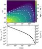 |
Fig. 1 Gas disk structure. Top panel: total hydrogen number density n⟨ H ⟩. The height of the disk z is scaled by the radius r. The white dashed contours correspond to the density levels shown in the colour bar. Bottom panel: total vertical hydrogen column number density N⟨ H ⟩ ,ver as a function of radius where on the right-hand side also the scale for the surface density Σ in g cm-2 is given. |
2.1.2. Dust disk structure
We assume a dust to gas mass ratio of δ = 0.01, which also determines the total dust mass. However, due to dust-evolution processes such as dust growth, dust settling, and drift (see e.g. Birnstiel et al. 2012), the dust density structure in a protoplanetary disk does not necessarily follow the gas density structure.
We account for this by including a dust-size distribution with a minimum dust grain size of amin = 0.05 μm and a maximum grain size of amax = 3000 μm. The size distribution itself is given by a simple power-law f(a) ∝ a− apow with apow = 3.5 (Mathis et al. 1977). Dust settling is incorporated by applying the method of Dubrulle et al. (1995), using a turbulent mixing parameter of αsettle = 10-2. This results in a grain size and gas-density dependent dust scale height and the dust to gas mass ratio varies within the disk. For example, at r = 100 au the local dust to gas mass ratio varies from δlocal ≈ 0.1 close to the midplane to values δlocal ≲ 0.001 in the upper layers of the disk. We note that the total dust to gas mass ratio δ stays the same (for more details see Woitke et al. 2016). We use porous grains composed of a mixture of amorphous carbon and silicate (see Table 1). The resulting dust grain density is ρgr = 2.1 g cm-3. Our model does not account for possible radial drift of large dust particles (see Sect. 4.3 for a discussion).
In PRODIMO, the same dust model is consistently used for the radiative transfer, including X-rays and the chemistry. For more details on the dust model and opacity calculations, see Woitke et al. (2016), Min et al. (2016).
2.1.3. Chemical network
Our chemical network is based on the gas-phase chemical database UMIST 2012 (McElroy et al. 2013) where we only use a subset of reactions according to our selection of species. Additionally to the gas phase reactions from the UMIST database we include detailed X-ray chemistry (Meijerink et al. 2012), charge exchange chemistry of PAHs (Polycyclic aromatic hydrocarbons, Thi et al. 2014, 2017), excited H2 chemistry, H2 formation using the analytical function of Cazaux & Tielens (2002, 2004) and adsorption and thermal, photo, and cosmic-ray desorption of ices (including PAHs). Dust surface chemistry is not included in our model.
The chemical network used here is described in detail in Kamp et al. (2017). We used their so-called large chemical network which consists of 235 chemical species (64 of them are ices) and 3143 chemical reactions. The element abundances are listed in Kamp et al. (2017). The element abundances correspond to the group of low metal abundances (e.g. Graedel et al. 1982; Lee et al. 1998). Further details concerning the chemistry of HCO+ and N2H+ and the used binding energies are given in Rab et al. (2017b).
To solve for the chemical abundances, we used the steady-state approach. In Woitke et al. (2016) and Rab et al. (2017b) comparisons of time-dependent and steady-state chemistry models are presented, which show that in our models steady-state is reached within typical lifetimes of disks in most regions of the disk. In Rab et al. (2017b) it is shown that the assumption of steady-state is well justified for HCO+ and N2H+ (see also Aikawa et al. 2015). The resulting differences between the steady-state and time-dependent models in the radial column density profiles of the molecular ions are not significant for our study.
Dust models.
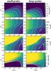 |
Fig. 2 Large grains (left column) and small grains (right column) disk model. From top to bottom the dust density, dust temperature, gas temperature and the disk UV radiation field χ in units of the Draine field are shown. The dashed contours in each plot correspond to the levels shown in the respective colour bar. The additional contours in the UV plots (bottom row) indicate where the radial (red solid line) and vertical (black solid line) visual extinctions are equal to unity. For both models, the same gas density structure as shown in Fig. 1 is used. |
2.2. Model groups
2.2.1. Dust models
For our investigations of the impact of the dust on the X-ray radiative transfer and on the molecular column densities we use three different dust-size distributions. All three distributions have the same dust composition as listed in Table 1. The parameters varied are amin, amax, and apow. In all three dust models the gas density structure is the same as described in Sect. 2.1.1 and the total dust to gas mass ratio is δ = 0.01. The details of the dust models are provided in Table 2.
The small grains model (SG) includes only a single dust size with a = 0.1 μm and no dust settling. Although such a dust model is likely not a good representation for the conditions in protoplanetary disks, is is useful as a reference and to show the impact of the dust on the X-ray radiative transfer and chemical disk structure.
The medium grain and large grain models are more appropriate in the context of grain growth and dust settling (see Sect. 2.1.2). Although, such dust models are a simplified representation of dust evolution in disks (Birnstiel et al. 2012; Vasyunin et al. 2011; Akimkin et al. 2013; Facchini et al. 2017), they still provide insight into the role of dust for the chemistry and X-ray radiative transfer. The main difference of the medium and large grain model is the amount of small particles. In the medium grain model about 10% of the total dust mass is in grains with a ≤ 1 μm, whereas in the large grain models it is only about 1.5%. Both models include dust settling as described in Sect. 2.1.2.
Most relevant for the chemistry is the total dust surface area per hydrogen nucleus (i.e. for the freeze-out of molecules). The dust surface area varies by about two orders of magnitude in our models (Table 2, see also Woitke et al. 2016; Rab et al. 2017a for details).
In Fig. 2 we show the dust density structure, the dust and gas temperature and the local UV radiation field in the disk, for the small grains and large grains model. The main difference in the dust models is the visual extinction AV, which significantly affects the dust temperature structure and the local disk radiation field.
2.2.2. Cosmic rays
There is some uncertainty about how many of the cosmic rays actually reach the disk of T Tauri stars. Similar to the Sun, the stellar wind of young stars, which might be significantly stronger compared to the Sun, can power a heliosphere-like analog which is called a “T Tauriosphere”. The existence of such a T Tauriosphere might reduce the cosmic-ray ionization rate in the disk by several orders of magnitude (Cleeves et al. 2013a).
To account for this, we use two different cosmic-ray input spectra; one is the canonical local ISM cosmic-ray spectrum (Webber 1998) and the second is a modulated spectrum which accounts for the suppression of cosmic-rays by a heliosphere. For the latter we use the “Solar Max” spectrum of Cleeves et al. (2013a). To calculate the cosmic-ray ionization rate we use the fitting formula of Padovani et al. (2013) and Cleeves et al. (2013a). The ISM cosmic-ray spectrum gives a cosmic-ray ionization rate per hydrogen nucleus of ζCR ≈ 10-17 and the Solar Max spectrum gives ζCR ≈ 10-19, which is consistent with the upper limit of the total H2 ionization rate in TW Hya derived by Cleeves et al. (2015). We call these two model groups “ISM cosmic rays” and “low cosmic rays”, respectively.
2.3. X-ray radiative transfer
For the X-ray radiative transfer (RT) we extended the already available radiative transfer module of PRODIMO to the X-ray wavelength regime. The 2D radiative transfer problem including scattering is solved with a ray-based method and a simple iterative scheme (Λ-iteration). The radiative transfer equation is solved for a coarse grid of wavelengths bands. For each band the relevant quantities (e.g. incident intensities, opacities) are averaged over the wavelength range covered by each band. The details of this method are described in Woitke et al. (2009). For the X-ray regime we find that about 20 wavelength bands are sufficient to represent the energy range of 0.1−20 keV used in our models. Besides the stellar radiation also interstellar radiation fields (UV and X-rays) are considered. For the interstellar radiation fields we assume that the disk is irradiated isotropically.
The X-ray RT module provides the X-ray radiation field for each point in the disk as a function of wavelength. Those values are used in the already available X-ray chemistry module of PRODIMO to calculate the X-ray ionization rate for the various chemical species. The X-ray chemistry used in this paper is the same as presented in Aresu et al. (2011) and Meijerink et al. (2012). As the chemistry influences the gas composition which in turn determines the gas opacities, we iterate between the X-ray RT and the chemistry. For each X-ray radiative transfer step the chemical abundances are kept fixed where for each chemistry step the X-ray ionization rates are fixed. We find that typically three to five iterations are required until convergence is reached.
2.3.1. X-ray scattering
Compton scattering, which reduces to Thomson scattering at low energies, is the dominant scattering process in the X-ray regime. The anisotropic behaviour of Compton scattering is treated via an approximation by reducing the isotropic scattering cross-section by a factor (1−g), where g = ⟨ cosθ ⟩ is the asymmetry parameter and θ is the scattering angle (see also Laor & Draine 1993). We use this approach for both the gas and the dust scattering cross-sections. We call this reduced cross-section the pseudo anisotropic (pa) scattering cross-section. g is zero for isotropic scattering and approaches unity in case of strong forward scattering. We apply this approach because the treatment of anisotropic scattering in a ray-based radiative transfer code is expensive, in contrast to Monte Carlo radiative transfer codes. Although this method is a simple approximation, it is very efficient and we find that our results concerning X-ray gas radiative transfer and the X-ray ionization rate are in reasonably good agreement with the Monte Carlo X-ray radiative transfer code MOCASSIN (see Appendix B).
2.3.2. X-ray gas opacities
For the X-ray gas opacities we used the open source library xraylib2 (Brunetti et al. 2004; Schoonjans et al. 2011). This library provides the X-ray absorption and scattering cross-sections (Rayleigh and Compton scattering) for atomic and molecular species. Concerning the X-ray gas absorption cross-section we find that the cross-section provided by xraylib are similar to the commonly used X-ray absorption cross-section of Verner & Yakovlev (1995), Verner et al. (1996).
For the calculation of the X-ray gas opacities we used the same low-metal element abundances as are used for the chemistry (see Sect. 2.1.3). As a consequence of the strong depletion of heavy metals (Na, Mg, Si, S, and Fe) by factors of 100 to 1000 compared to solar abundances, most of the absorption edges at higher energies (EX> 1 keV) disappear and the gas phase opacities in this regime are mostly dominated by hydrogen and helium (see also Bethell & Bergin 2011).
We note that we do not treat the depletion of gas-phase element abundances and the dust composition, which determines the element abundances in solids, consistently. Our approach here is to use the same dust properties (i.e. grain sizes, opacities) for the whole wavelength regime (X-ray to mm) considered in the radiative transfer modelling (see also Sect. 2.3.3 and Appendix A). The chosen dust opacities are well suited for modelling of protoplanetary disks as discussed in Woitke et al. (2016). However, for the dust compositions and the dust to gas mass ratio used in this work the sum of the gas and dust X-ray opacities are consistent within a factor of two with pure gas-phase X-ray opacities using the solar element abundances of Lodders (2003).
2.3.3. X-ray dust opacities
In the literature, only X-ray optical constants for astronomical silicates and carbon are available (Draine 2003). However, for protoplanetary disks often a mixture of different dust species is used.
We implemented the method of Draine (2003) to calculate X-ray optical constants for various dust compositions. This method uses the available optical constants, or more precisely the dielectric function, for the ultraviolet to the millimetre wavelength range and additionally the atomic gas phase photo-electric cross-sections for the X-ray regime. With this, the imaginary part of the complex dielectric function can be constructed from the X-ray to the millimetre regime. Via the Kramers-Kronig relation the real part of the dielectric function can be calculated knowing the imaginary part.
To be consistent with Draine (2003) we use the photo-electric cross-sections from Verner et al. (1996) to construct the imaginary part of the dielectric function. However, in contrast to Draine (2003) we do not include any additional measured data for the K edge absorption profiles (e.g. for graphite). The details of the absorption edges are less important here, as we are mainly interested in the resulting X-ray ionization rate which is an energy-integrated quantity.
In Fig. 3 we compare the optical constants for astronomical silicates (MgFeSiO4 composition) calculated via the above described method to the original optical constants provided by Draine (2003). The deviations of our results from the Draine (2003) data are likely a consequence of our simplified treatment of absorption edges. However, our approach is sufficient for deriving X-ray ionization rates.
By using these newly available optical constants we calculated the X-ray dust opacities with a combination of the Mie-theory, the Rayleigh-Gans approximation (Krügel 2002) and geometrical optics (Zhou et al. 2003) similar to Draine (2003) and Ercolano et al. (2008a). Also here we use the pseudo anisotropic scattering cross-sections in our calculations (see Sect. 2.3.1).
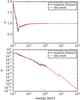 |
Fig. 3 Optical constants (n,k) for astronomical silicates in the X-ray regime. n (top panel) is the real and k (bottom panel) the imaginary part of the complex refractive index. The red solid lines show the results from this work and the black solid lines show the results from Draine (2003). |
In Fig. 4 we show the dust extinction (sum of absorption and scattering cross-sections) and the scattering cross-sections per hydrogen nucleus for three examples of dust size distributions and compositions, in a similar way as presented in Draine (2003). For comparison we also show the gas cross-section for the initial elemental abundances used in our models (low metal abundances, see Kamp et al. 2017), assuming that all hydrogen is molecular and all other elements are present as neutral atoms. For all cases shown in Fig. 4 we assumed a dust to gas mass ratio of 0.01.
The first panel in Fig. 4 shows the results for an MRN (Mathis, Rumpl, Nordsieck; Mathis et al. 1977) size distribution (amin = 0.005 μm, amax = 0.25 μm, and apow = 3.5) for pure astronomical silicates (Draine 2003). Although we do not use such a dust size distribution in our disk model the results are shown for reference. A comparison with Fig. 6 of Draine (2003) shows that our results are in good qualitative agreement with their results. However, Draine (2003) considered two individual dust populations with different dust compositions and size distributions; astronomical silicates and very small carbonaceous grains, the latter are not considered here. As a consequence, the carbon absorption edge at around 0.3 eV is missing in our MRN dust model.
Figure 4 clearly shows that for energies below 1 keV, the gas is the main opacity source even for the case of small grains. For higher energies dust becomes the dominant opacity source in the X-ray regime. However, considering a dust size distribution more typical for protoplanetary disks (amin = 0.05 μm, amax = 3000 μm, and apow = 3.5)‚ the dust extinction becomes only important for energies ≳4 keV. However, Fig. 4 also shows that the dust scattering cross-section is significantly reduced if the g factor approximation is applied. The scattering phase function for dust is strongly forward peaked resulting in a g factor very close to unity (i.e. small scattering angle Draine 2003). The main consequence is that dust scattering is insignificant for disks as it does not produce a diffuse radiation field as most photons are simply forward scattered (Bethell & Bergin 2011).
The gas scattering cross-section is nearly independent of energy and becomes the dominant opacity source for energies EX ≳ 5 keV. The scattering phase function of the gas is not strongly forward peaked as X-ray photons are mainly scattered by the electrons bound to hydrogen or helium. However, there is a slight decrease in the scattering cross-section with energy as Compton scattering becomes more anisotropic for higher energies, and in our simplified model this results in a reduced scattering cross-section.
We note that in our model the dust is simply an additional opacity source and we neglect any real interaction of X-rays with the dust, such as ionization or heating. The interaction of X-rays with solids is a very complex process (see e.g. Dwek & Smith 1996). Besides heating (e.g. Laor & Draine 1993) and ionization (Weingartner & Draine 2001), recent experiments indicate also possible dust amorphization by soft and hard X-rays (Ciaravella et al. 2016; Gavilan et al. 2016). However, we focus here on the X-ray ionization of the gas component and a detailed investigation of the impact of X-rays on the dust component is beyond the scope of this paper.
Our chemical model also includes PAHs (see Sect. 2.1.3). In Appendix C we show that the expected X-ray absorption cross-sections for PAHs are too low to play a significant role in the attenuation of X-ray radiation. As our focus here is on the X-ray ionization rates, a detailed modelling of the interaction of X-rays with PAHs is not considered.
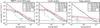 |
Fig. 4 X-ray cross-sections for the gas (black lines) and dust (blue and red lines) per hydrogen nucleus for three different dust-size distributions. The solid lines show the extinction (absorption+scattering) cross section and the dashed lines are the scattering cross sections. The left panel is for the MRN size distribution (Mathis et al. 1977) using pure astronomical silicates (Draine 2003). The two other panels are for the small and large grains dust models (see Sect. 2.2.1). For the dust, the red lines are for isotropic and the blue lines for pseudo anisotropic (pa) scattering (see Sect. 2.3.2). The pseudo anisotropic scattering values (blue dashed lines) are multiplied by a factor of 1000. The shown gas cross-sections are the same in all three panels. |
2.3.4. Stellar X-rays
To model the X-ray emission of T Tauri stars we assume that the origin of the emission is close to the stellar surface (see e.g. Ercolano et al. 2009) and place the source of the emission on the star. The spectral shape of the emission is modelled with an isothermal bremsstrahlung spectrum (Glassgold et al. 2009; Aresu et al. 2011) of the form 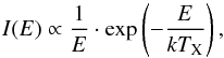 (4)where E is the energy in keV, I is the intensity, k is the Boltzman constant and TX = 2 × 10⁷ K is the plasma temperature. We considered an X-ray energy range of 0.1−20 keV for the stellar spectrum. The spectrum is normalized to a given total X-ray luminosity LX in the range 0.3−10 keV, as such an energy range is typical for reported observed X-ray luminosities (e.g. Güdel et al. 2007a).
We note that it is also possible to use a more realistic thermal line plus continuum X-ray spectrum as input in PRODIMO (see Woitke et al. 2016). However, as we do not model here a particular source, we use Eq. (4), which is a reasonable approximation for the general shape of observed X-ray spectra (Glassgold et al. 2009; Woitke et al. 2016).
2.3.5. X-ray background field
A star embedded in a young cluster likely receives X-ray radiation from the other cluster members. In Adams et al. (2012) typical flux values for such a cluster X-ray background field (XBGF) are derived, where the values depend on the cluster properties (e.g. number of cluster members) and the position of the considered target within the cluster. Such a cluster background field is probably one to two orders of magnitude stronger than the diffuse extragalactic background field (Adams et al. 2012).
In Adams et al. (2012) only the total flux or energy averaged values of the XBGF are considered and no detailed X-ray radiative transfer method is applied. Here we included the XBGF in the energy dependent X-ray radiative transfer module. To do this we modelled the spectrum of the background field in the same way as the stellar X-ray spectrum. We used an isothermal bremsstrahlung spectrum (Eq. (4)) with TX = 2 × 10⁷ K (kTX ≈ 1.7 keV) and normalized the spectrum to the given total flux in the energy range 0.1−20 keV. We assumed that the disk is irradiated isotropically by the XBGF.
Adams et al. (2012) estimated a characteristic flux level for a cluster X-ray background field (XBGF) of FXBGF = 1−6 × 10⁻⁵ erg cm-2 s-1. As discussed by Adams et al. (2012) variations from cluster to cluster and also between single cluster members (i.e. location within the cluster) can be significant. Therefore we consider here flux levels for the XBGF in the range FX = 2 × 10⁻⁶−2 × 10⁻⁴ erg cm-2 s-1, including the benchmark value of 2 × 10⁻⁵ from Adams et al. (2012). These values roughly cover the width of the X-ray background flux distributions derived by Adams et al. (2012). We note that we considered here a slightly wider X-ray energy range than Adams et al. (2012), who used 0.2−15 keV. Therefore the given total flux levels differ slightly; for example FX(0.1−20 keV) = 2 × 10⁻⁵ erg cm-2 s-1 corresponds to FX(0.2−15 keV) ≈ 1.4 × 10⁻⁵ erg cm-2 s-1.
Adams et al. (2012) assumes that there is no absorption of X-rays within the cluster. However, absorption of soft X-rays (E ≲ 1 keV) is possible, either by material between the star and the disk (see Ercolano et al. 2009) or the interstellar medium itself. To account for such a scenario in a simple way we also used input spectra with low-energy cut-offs of 0.3 and 1 keV, respectively (see Sect. 3.2.2).
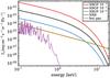 |
Fig. 5 X-ray background field spectra. The black solid line shows a cluster X-ray background field as proposed by Adams et al. (2012) with a flux of 2 × 10⁻⁵ erg cm-2 s-1 modelled with a bremsstrahlungs spectrum with TX = 2 × 10⁷K. The red and blue solid lines are for fluxes ten times higher and lower, respectively. For comparison we also show the diffuse extragalactic X-ray background field (XRB, brown solid line) using the fits described in Fabian & Barcons (1992) and a hot-gas spectrum (magenta line) from, for example, Supernova remnants (see Tielens 2005 chap. 1; Slavin & Frisch 2008). |
In Fig. 5 we show our XBGF spectra and additionally the spectrum measured for the diffuse extragalactic background field (Fabian & Barcons 1992) and a “hot gas” spectrum (e.g. produced by supernova remnants Tielens 2005). This figure shows that typically the cluster XBGF will dominate the X-ray background flux impinging on the disk.
3. Results
Our results are presented in the following way. In Sect. 3.1 we show the impact of scattering, dust opacities, and X-ray background fields on the X-ray disk ionization rate ζX. In Sect. 3.2 we present the molecular column densities of HCO+ and N2H+ for our three different dust models and for models with and without X-ray background fields.
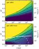 |
Fig. 6 X-ray ionization rate ζX for the 2D disk structure. Top panel: model with only gas absorption. Bottom panel: model with gas absorption and scattering. The white solid contour line shows N⟨ H ⟩ ,rad = 2 × 1024 cm-2, which corresponds roughly to the X-ray scattering surface. Below this surface ζX starts to be dominated by scattered X-ray photons. The white and red dashed lines show N⟨ H ⟩ ,ver = 2 × 1022 cm-2 and N⟨ H ⟩ ,ver = 2 × 1024 cm-2, respectively. |
3.1. X-ray disk ionization rates
In PRODIMO the X-ray ionization rate is calculated individually for the single atoms and molecules (see Meijerink et al. 2012 for details). ζX used in the following is simply the sum of the ionization rates of atomic and molecular hydrogen (we use a similar definition to Ádámkovics et al. 2011). We note that we define ζX per hydrogen nucleus, which is a factor of two lower compared to the ionization rate per molecular hydrogen. For all models discussed in this section LX = 1030 erg s-1, if not noted otherwise.
3.1.1. Impact of X-ray scattering
X-ray scattering is already a quite common ingredient in protoplanetary disk modelling codes (e.g. Igea & Glassgold 1999; Nomura et al. 2007; Ercolano et al. 2008a; Ercolano & Glassgold 2013; Cleeves et al. 2013a). In this Section we want to compare our results concerning scattering to some of those models. We also briefly discuss the importance of X-ray scattering for ζX considering both stellar X-rays and X-ray background fields.
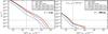 |
Fig. 7 X-ray ionization rate ζX vs. vertical column density N⟨ H ⟩ ,ver at disk radii of 1 au (left panel) and 100 au (right panel), respectively. The dashed lines show models with X-ray gas opacities only, where the purple line is for pure absorption and the orange line for absorption plus scattering. The solid lines are for models including X-ray dust opacities (absorption+scattering), where results for the small grains (SG, blue), medium grains (MG, red) and large grains (LG, black) dust models are shown. The vertical grey line in both plots indicates the scattering surface at N⟨ H ⟩ ,rad = 2 × 1024 cm-2 (see also Fig. 6); at the right hand side of this line ζX is dominated by scattered high-energy photons. The horizontal lines mark the cosmic-ray ionization rates for the ISM (ζCR ≈ 10-17), and low cosmic-ray case (ζCR ≈ 10-19 s-1). |
 |
Fig. 8 X-ray ionization rate ζX for the three different dust models including X-ray opacities for the gas and the dust. The white solid contour shows N⟨ H ⟩ ,rad = 2 × 1024 cm-2, which corresponds to the scattering surface. The dashed white contour shows where ζX is equal to ζX,abs of the gas absorption only model. Above this line ζX ≤ ζX,abs (additional absorption by the dust) and below, ζX>ζX,abs (scattering). |
In Fig. 6 we show ζX for the whole 2D disk structure for a model with X-ray gas absorption only and a model including scattering. In these models dust is not considered as an X-ray opacity source. The same models are also included in Fig. 7 where ζX is plotted as a function of vertical hydrogen column density N⟨ H ⟩ ,ver at radii of 1 and 100 au distance from the central star.
As discussed already in Igea & Glassgold (1999) and Ercolano & Glassgold (2013) it is possible to define a single scattering surface in the disk, because the scattering cross-section of the gas component is nearly constant over the whole X-ray energy range (see Fig. 4). A scattering optical depth of unity is reached at a hydrogen column density of N⟨ H ⟩ ≈ 2 × 1024 cm-2 (see Fig. 4 and Igea & Glassgold 1999). For stellar X-rays the radial column density defines the location of the scattering surface in the disk (see Fig. 6). Below the scattering surface, the X-ray ionization rate is dominated by scattered X-rays. We want to note that the location of the scattering surface depends on the location of the X-ray source. For example, in the models of Igea & Glassgold (1999) and Ercolano & Glassgold (2013), the central X-ray source is located 12 R⊙ above and below the star. Compared to our model where the X-ray source is the star itself, the scattering surface moves to deeper layers in the disk as the radial column density seen by stellar X-rays is reduced (see also Appendix B). This can cause differences in ζX by about an order of magnitude in vertical layers close to the scattering surface (Igea & Glassgold 1999). In terms of vertical column density the scattering surface is located at N⟨ H ⟩ ,ver ≈ 2 × 1022 cm-2 for r ≲ 50 au, but drops rapidly to lower vertical column densities due to the disk structure (see Fig. 6).
An X-ray background field irradiates the disk isotropically. In Fig. 6 we also mark N⟨ H ⟩ ,ver ≈ 2 × 1024 cm-2 which roughly corresponds to the scattering surface for X-ray radiation entering the disk vertically (perpendicular to the midplane). This indicates that scattering is of less importance for X-ray background fields, as only in the region with N⟨ H ⟩ ,ver ≳ 2 × 1024 cm-2 (i.e. r ≲ 10 au) can scattering become significant. However, in that region stellar X-rays will dominate the disk radiation field anyway (see Sect. 3.1.3). Test models with and without X-ray scattering indeed showed that scattering is negligible for the case of an isotropic X-ray background radiation source.
In Fig. 7, ζX is also shown for models with and without scattering. This figure shows that at high column densities, ζX is dominated by X-ray scattering, whereas at low column densities, ζX is not significantly affected by scattering and is dominated by direct stellar X-rays. The reason is that the scattering cross-section becomes only comparable to the absorption cross-section for X-ray energies E ≳ 5 keV (see Fig. 4). This means that mainly the energetic X-ray photons are scattered towards the midplane of the disk, where above the scattering surface ζX is dominated by the softer X-rays which are not efficiently scattered. This is consistent with other X-ray radiative transfer models (e.g. Igea & Glassgold 1999; Ercolano & Glassgold 2013; Cleeves et al. 2013b).
3.1.2. Impact of dust opacities
In Fig. 8 we show the X-ray ionization rate for models with three different dust size distributions: small grains, medium grains and large grains (see Sect. 2.2.1). In these models both the gas and dust opacities are considered in the X-ray RT, but the X-ray gas opacities are the same in all three dust models. To compare ζX to models without X-ray dust opacities they are also included in Fig. 7.
As already mentioned, scattering of X-rays by dust can be neglected due to the strongly forward peaked scattering phase function (see Sect. 2.3.3). As the dust acts only as an additional absorption agent, ζX is reduced wherever the dust opacity becomes similar or larger than the gas opacity. This is the case particularly for high X-ray energies (see Fig. 4) but depends on the chosen dust properties. In the case of small grains, dust absorption dominates the X-ray opacity for X-ray energies EX ≳ 1 keV. As a consequence ζX drops by about an order of magnitude and more, compared to the model with gas opacities only (see Fig. 7). For the medium and large grain models the impact of dust is much less severe. For the medium grains, dust extinction becomes relevant for EX ≳ 3 keV and for the large grains, it only becomes relevant for EX ≳ 10 keV. In the large grains model, however, gas extinction remains always higher than dust absorption (see Fig. 4).
Our results imply that dust extinction plays an important role for young disks, whereas for evolved disks with large grains, X-rays can penetrate deeper. In evolved disks, only the most energetic X-rays are affected as the gas opacity drops rapidly with energy. Therefore the impact on ζX is the largest in the deep, high-density layers of the disk where ζX is dominated by high-energy X-rays. In young objects, where the disk is still embedded in an envelope, small grains can be important and should be included in X-ray radiative transfer models. We will investigate such a scenario based on the Class I PRODIMO model presented in Rab et al. (2017a) in a future study.
3.1.3. Impact of X-ray background fields
The importance of X-ray background fields for disks was estimated analytically by Adams et al. (2012). They find that the X-ray background flux can be larger than the stellar X-ray flux for disk radii r ≳ 14 au, assuming a geometrically flat disk and a typical disk impact angle for the stellar radiation. Their estimated radius corresponds to the radius where the stellar and interstellar X-ray flux become equal. However, attenuation by the disk itself was not taken into account (i.e. they compared the stellar and background X-ray fluxes at the disk surface).
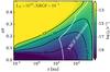 |
Fig. 9 X-ray ionization rate ζX for a model with LX = 1029 erg s-1 and FXBGF = 2 × 10⁻⁵ erg cm-2 s-1 (i.e. the benchmark values of Adams et al. 2012). The white solid contour line encloses the region where the XBGF dominates ζX (i.e. ζX,XBGF ≥ ζX, ∗). |
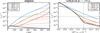 |
Fig. 10 X-ray ionization rate in the midplane (left panel) and for a vertical cut at r = 150 au (right panel) for models with fixed stellar X-ray luminosity (LX = 1030 erg s-1) but varying X-ray background fields with fluxes of 2 × 10⁻⁴ (blue), 2 × 10⁻⁵ (brown) and 2 × 10⁻⁴ erg cm-2 s-1 (red); the black lines are for the model without an XBGF. The solid lines are for the full X-ray spectra (0.1−20 keV); the dotted and dashed lines correspond to models with a low-energy cut-off at 0.3 keV and 1 keV, respectively. The horizontal lines mark the cosmic-ray ionization rates for the ISM (ζCR ≈ 10-17), and low cosmic-ray case (ζCR ≈ 10-19 s-1). In the right panel, the vertical grey solid line indicates the scattering surface at N⟨ H ⟩ ,rad = 2 × 1024 cm-2 (see also Fig. 7). |
In Fig. 9 we show ζX for our full 2D disk model using LX = 1029 erg s-1 and an X-ray background flux of FXBGF = 2 × 10⁻⁵ erg cm-2 s-1 (these are the values used by Adams et al. 2012 for their benchmark case). We mark the region of the disk where the X-ray background field dominates ζX (i.e. ζX,XBGF ≥ ζX, ∗). In the midplane of the disk (z = 0) the XBGF dominates for r ≳ 20 au. Assuming a geometrically flat disk, the XBGF dominates in our model for r ≳ 15 au (we simply projected the smallest radius at the maximum height, where the XBGF dominates, to the midplane). For the same XBGF but LX = 1030 erg s-1 we find that the XBGF dominates for r ≳ 30 au for a geometrically flat disk and r ≳ 45 au for the midplane of our 2D model. Those radii are consistent with the analytical estimates of Adams et al. (2012).
In Fig. 10 we show ζX in the midplane and for a vertical cut at r = 150 au for models with different XBGF fluxes and a fixed stellar X-ray luminosity of LX = 1030 erg s-1. Additionally we show models with a low-energy cut-off for the stellar and XBGF spectrum at 0.3 and 1 keV, respectively. With this low-energy cut-off we simulate (in a simple way) a possible absorption of the X-rays before they actually impinge on the disk. Such an absorption can happen by material close to the star (e.g. accretion columns Grady et al. 2010) for the stellar X-rays and in case of the X-ray background field additional extinction due to the interstellar medium is also possible. The corresponding absorption columns required for those cut-offs are N⟨ H ⟩ ≈ 1021 cm-2 for 0.3 keV and N⟨ H ⟩ ≈ 1022 cm-2 for 1 keV (see Fig. 4 and Ercolano et al. 2009).
As seen from the left panel of Fig. 10, ζX at the outer radius of the disk can be as high as 10-14 s-1 but strongly depends on the assumed low-energy cut-off. Adams et al. (2012) also estimated ζX for their benchmark X-ray background field (FXBGF = 2 × 10⁻⁵ erg cm-2 s-1) assuming an average X-ray photon energy of EX = 1 keV; they find ζX = 8 × 10-17 s-1. This is similar to our model with the 0.3 keV low-energy cut-off.
The low-energy cut-off has no significant impact on the radius down to which the XBGF dominates ζX. For these high-density regions, only the most energetic X-rays, which are not affected by the low-energy cut-off, are of relevance. However, as seen from Fig. 10 a possible absorption of the XBGF photons before they reach the disk has a significant impact for radii r ≳ 200 au and at higher layers of the disk. For the 1 keV-cut-off, ζX can be lower by more than an order of magnitude compared to the reference model with a minimum X-ray energy of 0.1 keV.
More important than the value of ζX at the outer disk radius is the value at higher densities where the actual emission from molecular ions originates. From Fig. 10 we can see that ζX drops already below the ISM cosmic-ray ionization rate at r ≈ 200 au even for the strongest XBGF considered. However, for the low cosmic-ray case, the XBGF can be the dominant high-energy ionization source in the midplane for radii as small as r ≈ 50 au. This is also seen in the right panel of Fig. 10; depending on the XBGF flux, ζX can reach values around 5 × 10-18 s-1 close to the midplane of the disk at r = 150 au.
3.2. Molecular ion column densities
In this section we show results for the radial column density profiles of the disk ionization tracers HCO+ and N2H+. We use these two molecules because they are the most commonly detected molecular ions in disks (e.g. Thi et al. 2004; Dutrey et al. 2007; Öberg et al. 2011a; Guilloteau et al. 2016) and because they trace different regions in the disk.
HCO+ and N2H+ are mainly formed via proton exchange of  with CO and N2, respectively. The main destruction pathway is dissociative recombination with free electrons, where the metals (e.g. sulphur) play a significant role as additional electron donors (e.g. Graedel et al. 1982; Teague et al. 2015; Kamp et al. 2013; Rab et al. 2017b). HCO+ and N2H+ are sensitive to high-energy ionization sources such as X-rays and cosmic-rays, because the formation of involves the ionization of H2 (15.4 eV ionization potential).
Besides free electrons, another efficient destruction pathway for N2H+ and HCO+ are ion-neutral reactions. N2H+ is efficiently destroyed by CO and therefore resides mainly in regions where gas phase CO is depleted (e.g. frozen-out). This makes it a good observational tracer of the CO ice line in disks (e.g. Qi et al. 2013; Aikawa et al. 2015; van’t Hoff et al. 2017). In the case of HCO+, gas phase water is the destructive reaction partner. Observations of protostellar envelopes indicate that HCO+ is indeed sensitive to the water gas phase abundances (e.g. Jørgensen et al. 2013; Bjerkeli et al. 2016; van Dishoeck et al. 2014). In disks this is more difficult to observe, due to the more complex structure and because the water snow line in disks is located at much smaller radii (r ≈ 1 au for a T Tauri star) compared to CO (r ≈ 20 au). However, HCO+ follows mainly the distribution of gas phase CO in the disks, whereas N2H+ traces regions where CO is frozen-out (i.e. where the temperature is ≲25 K).
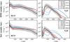 |
Fig. 11 HCO+ (left column) and N2H+ (right column) radial column density profiles for models with different dust-size distributions: small grains (SG, blue), medium grains (MG, red), and large grains (LG, black). The dashed lines are for models where only the gas component is considered in the X-ray RT, where the solid lines show models where both X-ray gas and dust opacities are included. The ISM cosmic-ray models are shown in the top row and the low cosmic-ray models are shown in the bottom row. The grey shaded area marks a difference of a factor three in N with respect to the reference model (LG gas+dust). |
For the abundance of the molecular ions, the so called sink-effect for CO and N2 is also of relevance. The main mechanism of the sink effect is the conversion of CO and N2 to less volatile species which freeze out at higher temperatures or remain on the dust grains. This can happen via surface chemistry and/or via dissociation of neutral molecules by He+ (e.g. Aikawa et al. 1996, 2015; Bergin et al. 2014; Cleeves et al. 2015; Helling et al. 2014; Furuya & Aikawa 2014; Reboussin et al. 2015). The main consequence of the sink effect is the depletion of gas phase CO and N2 in regions with temperatures above their respective sublimation temperatures. However, the efficiency of the sink effect is not very well understood as it depends on various chemical parameters (see Aikawa et al. 2015 for more details). In our model only the He+ sink-effect is considered.
Our model also includes excited H2 chemistry that opens up another formation pathway for HCO+. This formation pathway can be important close to the C+/ C/CO transition (see Greenwood et al. 2017 and Appendix D). The relevance of this pathway is discussed below.
The typical abundance structure for HCO+ and N2H+ in our reference model is presented in Rab et al. (2017b). Here we focus on the radial column densities because they can be more easily compared to observations and other thermo-chemical disk models.
3.2.1. Impact of dust grain size distributions on chemistry
In Fig. 11, we show the molecular ion column densities NHCO+ and NN2H+ for the three different dust models, small grains (SG), medium grains (MG), and large grains (LG) described in Sect. 2.2.1. For each dust model also both cases of cosmic-ray ionization rates, low and ISM cosmic rays, are shown (Sect. 2.2.2). Further we show models with and without X-ray dust opacities. All models shown in Fig. 11 have LX = 1030 erg s-1 and no X-ray background field.
It is clearly seen in Fig. 11 that neither for the medium grains nor for large grains does the inclusion of X-ray dust opacities have a significant impact on the molecular ion column densities. Only for N2H+ can a slight decrease on the column density be seen in the models with low cosmic rays (e.g. compare model MG gas with MG gas+dust). The column densities are not significantly affected by including X-ray dust opacities, as the strongest impact of the dust on ζX is limited to regions close to the midplane (see Fig. 7). There, CRs mostly dominate the molecular ion abundances as the X-ray ionization is typically ζX ≲ 10-19 s-1, even if dust opacities are not included. Further the contribution to the molecular ion column densities from regions close to the midplane is limited as the parent molecules of the ions are frozen out anyway. The situation is different for the SG model, where ζX is affected by the dust at all disk layers (see Fig. 7) and NHCO+ and NN2H+ can drop by factors of three to ten. This shows that it is justified, in case of HCO+ and N2H+, to neglect X-ray dust opacities for evolved disk dust populations but not necessarily for ISM-like dust.
Figure 11 also shows that, independent of the X-ray dust opacities, the dust grain size distributions themselves have a significant impact on the molecular column densities. In the SG model, the gas disk is more efficiently shielded from the stellar and interstellar UV radiation field but also the total dust surface per hydrogen nucleus increases significantly (see Table 2). This has two main consequences:
Firstly, the ionization of metals such as carbon and sulphur is significantly reduced. This causes a decrease in the number of free electrons available for the dissociative recombination with molecular ions. On the other hand the impact of the dust opacities on the X-ray disk radiation field (and on ζX) is less significant (SG model), or not significant at all (MG and LG model) compared to the impact of the dust on the UV radiation field. Consequently the abundance of the molecular ions increases in regions which are efficiently shielded from the UV radiation fields by the presence of small grains.
Secondly, the freeze-out and the sink effect become more important if the total dust surface increases. This reduces the abundance of molecular ions in high-density regions that are efficiently shielded from UV radiation (i.e. no photo-desorption).
These effects are best seen for NN2H+. Compared to the LG model, in the SG model the abundance of N2H+ is reduced close to the midplane of the disk due to the sink effect and freeze-out (i.e. lower gas phase abundance of the parent molecule N2) but increases in the outer and upper layers of the disk due to the shielding of the UV radiation by small grains (i.e. lower abundance of metal ions). This results in a shift of the NN2H+ peak to larger radii (r ≈ 150−200 au), and the peak is no longer tracing the radial CO ice line (which is at r ≈ 45 au in the SG model). For radii r ≲ 150 au, NN2H+ is now dominated by the N2H+ layer just below the C+/C/CO transition where the X-ray ionization rate is high enough so that N2H+ survives also in layers with gas phase CO (see Aikawa et al. 2015; van’t Hoff et al. 2017; Rab et al. 2017b). In contrast to the LG grain model, NN2H+ in the SG model can reach comparable or even higher values in the inner disk (r ≲ 100 au) compared to the peak value around r ≈ 150−200 au.
Aikawa et al. (2015) also used two different dust-size distributions (ISM-like and large grains) for their detailed study on N2H+ in protoplanetary disks. Their resulting column density profiles are very similar to what is shown in Fig. 11. In the chemical models of Dutrey et al. (2007) for DM Tau and LkCa 15 the peak in their NN2H+ profiles are at very large radii (r ≳ 400 au), which is likely due to their assumed single grain size of 0.1 μm. Cleeves et al. (2015) used a reduced dust surface area, compared to 0.1 μm grains, to model NN2H+ for TW Hya, however they also required a lower cosmic-ray ionization rate (ζCR ≈ 10-19 s-1) to match the observed sharp peak in NN2H+, located close to the CO ice line. A lower cosmic-ray ionization rate decreases the efficiency of the He+ sink effect. A strong impact of the low cosmic-ray ionization rate on the NN2H+ peak is not really seen in our models or in the models of Aikawa et al. (2015). This might be caused by differences in the time-scales for the sink effect (Bergin et al. 2014). In our LG model, steady-state for NN2H+ is already reached at a chemical age of approximately 1 Myr (see Rab et al. 2017b). For the SG models, a time-dependent test run with ISM cosmic rays showed that steady-state is only reached after 2−3 Myr in regions around the radial CO ice line, whereas at ≈1 Myr the NN2H+ peak is still tracing the radial CO ice line.
Despite the differences in the various chemical models, they all indicate that the sink effect plays a crucial role in the shape of the N2H+ radial column density profile. Further, only models accounting for dust growth are able to reproduce a sharp peak in the NN2H+ profile near the radial CO ice line as is observed for TW Hya (Qi et al. 2013; but see also Aikawa et al. 2015; van’t Hoff et al. 2017 for a discussion on the robustness of NN2H+ as a CO ice line tracer). This is consistent with dust observations clearly indicating grain growth and dust settling in disks (e.g. Andrews & Williams 2005; Pinte et al. 2016). In any case, the chemical modelling results for NN2H+ indicate that N2H+ is not only a tracer of the radial CO ice line but also for dust evolution in disks.
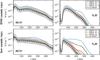 |
Fig. 12 Radial column density profiles for HCO+ and N2H+ with (coloured lines) and without (black lines) XBGF for the ISM (top row) and low (bottom row) cosmic-ray case. The dashed lines are for models with a low-energy cut-off of the X-ray spectra (stellar and XBGF) of 1 keV; for the solid lines the lowest X-ray energy is 0.1 keV. The grey shaded area marks a factor of three difference in N with respect to the models without XBGF (the solid black line). |
3.2.2. Impact of X-ray background fields on chemistry
To show the impact of X-ray background fields (XBGF) on the molecular column densities we compare in Fig. 12 models with LX = 1030 erg s-1 but varying XBGF fluxes. We also include models with a low-energy cut-off at 1 keV to show the impact of the possible absorption of soft X-rays before they reach the disk (see also Sect. 3.1.3). For each of these models the results for low and ISM cosmic rays are shown. For all models the large grains dust model is used.
For the case of the ISM cosmic-ray ionization rate, the impact of the XBGF on the column densities is limited. Only for models with the highest XBGF flux of 2 × 10⁻⁴ erg cm-2 s-1 do the column densities increase by more than a factor of three for radii r ≳ 250 au. Although the XBGF dominates the X-ray ionization rate down to r ≈ 20 au, ζX>ζCR is true only for r ≳ 200 au, and only for the case of the strongest XBGF (see Fig. 10).
The impact of the XBGF is much larger in the case of a low CR ionization rate. In that case the molecular ion column densities are generally lower compared to ISM CRs and the relative impact of the XBGF increases. However, the impact on NHCO+ remains limited; only for the strongest XBGF does NHCO+ increase by about a factor of five at most. For NN2H+ the picture is quite different. Due to the low CRs, the column densities for r ≳ 200 au are reduced by more than an order of magnitude compared to the ISM CRs models. In these regions the XBGF is now most effective and consequently NN2H+ increases significantly. For the strongest XBGF, NN2H+ increases by up to two orders of magnitude for r ≳ 200 au and reaches levels similar to the ISM CR models. The reason why N2H+ is more sensitive to the high-energy ionization sources is its location in the disk. Compared to HCO+, N2H+ is mainly located in deeper layers of the disk; below the CO ice line. In those layers, the ionization balance is mostly dominated by molecular ions, as the ionization of atomic metals by UV becomes less important.
In the models with a low-energy cut-off at 1 keV for the X-ray spectra, HCO+ is not affected by the XBGF even in the low CR model. Also the impact on NN2H+ is now weaker. NN2H+ is typically a factor of a few up to an order of magnitude lower compared to the models with a cut-off at 0.1 keV. Although we use the low-energy cut-off also for the stellar X-rays, such a drop in the column densities is not seen in the models without XBGFs. The reasons are the geometrical dilution of the stellar X-ray radiation and that the stellar X-rays have to penetrate the high radial and vertical column densities in the inner disk. The XBGF irradiates the disk isotropically and only has to penetrate the low column densities of the outer disk. Therefore also the low-energy X-rays can penetrate larger areas of the disk and have more impact on ζX in disk regions relevant for the molecular ions.
For HCO+ we actually also see a drop in the column density for r ≳ 400 au for the strongest XBGF. The reason for this is a lower CO abundance caused by X-ray photo-dissociation which is also included in our chemistry model. The CO abundance at r ≳ 450 au drops by factors of approximately three to five down to heights of z ≈ 20 au, which results in a drop of the HCO+ abundance by nearly an order of magnitude. The situation is similar for N2 and N2H+; however the abundance of N2H+ is already below 10-12.
As noted (Sect. 3.2), our model also includes chemistry of excited molecular hydrogen  . This opens up a formation channel for HCO+ via the ion-neutral reaction of with C+ (see Appendix D for details). In the inner disk, this reaction is only effective in a very thin layer at the C+/C/CO transition. However, in the outer disk for r ≳ 300 au this reaction becomes significant, as the C+/C/CO transition is not as sharp as in the inner disk. If this reaction is deactivated, we find that for such a model the slope of NHCO+ for r> 300 au becomes steeper. However, our findings concerning the impact of XBGFs are not significantly affected; NHCO+ becomes slightly more sensitive to XBGFs for r ≳ 300 au and X-ray photo-dissociation becomes less significant for NHCO+ at large radii where NHCO+ drops below 1010 cm-2 (r ≈ 400 au). The results for N2H+ are not affected by chemistry.
4. Discussion
4.1. Observational implications of X-ray background fields
Our results indicate that the molecular ion column densities in the outer disk are sensitive to X-ray background fields. At least for N2H+ the effect on the column density can be strong enough to be observable with modern (sub)millimetre telescopes like ALMA (Atacama Large Millimeter Array), NOEMA (NOrthern Extended Millimeter Array) and SMA (Submillimeter Array). However, our results also show that certain conditions, such as a strong XBGF and low CR ionization rates, are required.
The typical value for the X-ray background flux in young embedded clusters of 2 × 10⁻⁵ erg cm-2 s-1 corresponds to cluster member sizes with N< 3000, typical for clusters in the solar vicinity (Adams et al. 2012). However, this value drops to ≲10-5 erg cm-2 s-1 for smaller clusters with N ≈ 100, which is more typical for the Taurus star formation region; the X-ray XEST survey detected 136 X-ray sources (Güdel et al. 2007a). A typical disk in Taurus would only be affected by an XBGF if it were shielded efficiently from cosmic-rays (see Fig. 12). However, even in a small cluster some of the sources might experience a higher X-ray background flux depending on their location within the cluster (e.g. closer to the cluster centre; see Adams et al. 2012). To identify such sources, a large sample of spatially resolved N2H+ observations (see below) would be required. The current number of N2H+ detections in protoplanetary disks is less than ten (Dutrey et al. 2014) and it is therefore not surprising that signatures of XBGF have not yet been found.
Due to the rather poor knowledge concerning the impact of individual high-energy ionization sources on disk chemistry (see e.g. Rab et al. 2017b) and as only the stellar X-ray luminosity can be measured, it will certainly be challenging to discriminate the influence of XBGFs from the stellar high-energy ionization sources (X-rays and stellar energetic particles), cosmic-rays and radionuclide ionization. However, all these ionization sources are different in the way they irradiate the disk.
The stellar high-energy ionization sources have less impact on the outer disk; they need to penetrate the high densities in the inner disk and also experience geometric dilution as they irradiate the disk as a point source (see also Rab et al. 2017b). Cosmic rays irradiate the disk isotropically and therefore have an impact on the whole disk. Due to their high energies, CRs are only significantly absorbed in the inner disk (r ≲ 10 au) and provide therefore a nearly constant H2 ionization rate for the bulk of the disk material (this is similar for radionuclide ionization). In contrast to CRs, the XBGF experiences significant absorption by the disk material even in the outer disk. Those differences result in different shapes of the N2H+ radial column density profiles as is seen in Fig. 12. XBGFs make the profile shallower as the impact on the molecular column densities decreases for smaller disk radii (measured from the star). In contrast, a change in the CR ionization rate affects the radial column density profile at all radii.
In any case, modelling of spatially resolved N2H+ observations of disks is required to discriminate the contribution of XBGF to disk ionization. Such observations for T Tauri disks are still rare (Dutrey et al. 2007; Qi et al. 2013) but certainly will become more common in the near future due to the significant advances, in particular in terms of spatial resolution, of modern (sub)mm interferometers.
4.2. UV background fields and external photo-evaporation
For all models presented here we assumed the canonical value for the interstellar UV radiation of χISM = 1 (in units of the Draine field). This is a reasonable assumption for low-mass star formation regions as an enhanced UV background field would be mostly produced by massive stars with spectral types O, B, and A. In contrast to the UV field, the X-ray background field is mainly produced by X-ray emission of solar-like low-mass stars (see Adams et al. 2012). However, the presence of an enhanced UV background field certainly has an impact on the outer disk due to photo-dissociation of molecules, photo-desorption of ices and photo-ionization of metals (see e.g. Teague et al. 2015). These processes will reduce the abundances of molecular ions in the outer disk as their parent molecules are dissociated and metals like carbon and sulphur are ionized and will therefore dominate the ionization balance. Consequently, the presence of an enhanced UV background field will lower the impact of the XBGF on the outer disk molecular abundances. In high-mass star formation regions like Orion with UV background fields up to χISM ≈ 104, the UV field will most likely completely dominate the chemistry in the outer disk (Walsh et al. 2013; Antonellini et al. 2015).
There is evidence that already weak UV background fields χISM ≳ 4 can drive photo-evaporation of the outer disk (Haworth et al. 2017; but see also Adams 2010; Williams & Cieza 2011). Such a process is not included in our model. However, we do not expect a huge impact of photo-evaporation on our results. For the X-ray RT, mainly the column density matters, which photons have to penetrate until they reach the regions of the disk where the molecular ions become abundant. These column densities are not significantly affected if parts of the outer disk material slowly drift radially outwards.
On the other hand, XBGFs can act as an additional heating source for the outer disk and therefore could contribute to external disk photo-evaporation. We find that only the strongest X-ray background field with FXBGF = 2 × 10⁻⁴ erg cm-2 s-1 has a significant impact on the gas temperature in our models. In the midplane of the disk at r ≈ 500 au (n⟨ H ⟩ ≈ 4 × 105 cm-3), the gas temperature increases from about Tg ≈ 24 K to Tg ≈ 36 K, where for the canonical XBGF we find only an increase of about 2 K (always χISM = 1 is used). Those gas temperatures are lower than the typical temperatures reported by Facchini et al. (2016) derived from hydrodynamical disk photo-evaporation models with χISM ≥ 30. This indicates that in the presence of a modestly enhanced UV background field, XBGFs would play a rather minor role for external disk photo-evaporation. However, a more detailed investigation of the possible importance of XBGFs for external disk photo-evaporation is required to be more quantitative.
4.3. The role of dust evolution
The properties of the dust and its evolution has a significant impact on the chemical structure of the disk (e.g. Vasyunin et al. 2011; Akimkin et al. 2013; Woitke et al. 2016). Important dust evolution processes are dust growth, dust settling, and radial migration of (sub)mm sized grains. Individual disks likely will show different dust properties as dust evolution proceeds over time and also depends on various parameters such as the turbulence in the disk (see Birnstiel et al. 2016 for a recent review). Good knowledge of the dust disk (e.g. from continuum observations) is therefore crucial for modelling of molecular line emission of individual protoplanetary disks. In the following, we briefly discuss the impact of dust evolution on our results and possible shortcomings of our dust model.
In our modelling approach, we include methods to simulate dust growth and dust settling (see Sects. 2.1.2 and 2.2.1). The models with varying grain size distributions indicate a significant impact of the assumed grain size on the radial column densities of HCO+ and N2H+ (see Sect. 3.2.1). We also ran disk models using the large grains dust model but varied the degree of settling (i.e. no settling at all and strong settling with αsettle = 10-4). For the case of strong settling, the HCO+ and N2H+ column densities change at most by a factor of three where HCO+ is more sensitive than N2H+. In the non-settled disk model, only N2H+ is affected where the column density drops by about an order of magnitude around r = 100 au. However, the relative impact of X-ray background fields on the molecular column densities is similar to the models presented in Sect. 3.2.2 and consequently our conclusions concerning the impact of X-ray background fields are not affected. Nevertheless, for modelling of molecular observations of individual disks, it is also necessary to consistently model the dust component. The model presented here is well suited for such modelling, as the same dust model is used for the radiative transfer (X-ray to mm), the chemistry, and also for the calculation of synthetic observables such as spectral energy distributions and spectral line emission (see Woitke et al. 2016).
Not included in our model is the inward radial migration of large dust grains. Spatially resolved (sub)mm observations indicate that the radial extent of dust emission is significantly smaller than the molecular gas emission (for CO see e.g. de Gregorio-Monsalvo et al. 2013; Cleeves et al. 2016). However, models indicate that the difference in the extent of the dust- and gas-emitting areas might be an optical depth effect (Woitke et al. 2016; Facchini et al. 2017). Nevertheless, radial migration of large dust particles can have an impact on the molecular abundances in the outer disk as shown by Cleeves (2016) for CO. The models of Cleeves (2016) show that the depletion of large dust grains in the outer disk can increase the CO gas phase column density by about a factor of two compared to models without radial migration. This will likely also have an impact on the HCO+ and N2H+ column densities.
We do not expect that radial migration affects our general conclusions on the impact of X-ray background fields. The changes in the molecular ion abundances in the outer disk are purely driven by an increase of the X-ray ionization rate. It is unlikely that the X-ray ionization rate is strongly affected by the depletion of large dust grains in the outer disk, as in that case the X-ray opacities are dominated by the gas, similar to our large dust grains model (see Fig. 4). The impact of radial migration on the molecular ion abundances is an interesting aspect which certainly deserves more detailed investigation. However, such a study is beyond the scope of this paper.
Recent ALMA observations have shown azimuthally symmetric gap- and ring structures in the disk emission of (sub)mm sized dust grains (e.g. ALMA Partnership et al. 2015; Andrews et al. 2016; Isella et al. 2016). Although the dust depletion in the gaps has an impact on the molecular gas phase abundances (e.g. Teague et al. 2017), those rings are rather narrow (width ≲10 au, Pinte et al. 2016) and the global radial distribution of the molecular column densities remains intact. Therefore our main conclusions concerning the impact of X-ray background fields are not significantly affected by the presence of gaps.
5. Summary and conclusions
We introduced a new X-ray radiative transfer module for the radiation thermo-chemical disk code PRODIMO. This new module includes X-ray scattering and a detailed treatment of X-ray dust opacities, which can be applied to different dust compositions and dust size distributions. We investigated the importance of X-ray scattering, X-ray dust opacities, and X-ray background fields of embedded young clusters for the X-ray ionization rates by means of a representative T Tauri protoplanetary disk model. Further, we studied the impact of X-ray background fields on the disk chemistry, where we used the observed disk ionization tracers HCO+ and N2H+. Our main conclusions are:
-
For evolved dust-size distributions (e.g. including grain growth)X-ray opacities are mostly dominated by the gas; only forenergiesEX ≳ 5−10 keV do dust opacities become relevant. Consequently, the disk X-ray ionization rates are only reduced in high-density regions close to the midplane if dust opacities are included in the X-ray RT. For ISM-like dust-size distributions (i.e. maximum grain size ≲0.1 μm) the X-ray ionization rate is affected throughout the disk and is reduced by more than an order of magnitude due to efficient absorption of X-rays by the dust.
-
For a typical X-ray background flux, as expected for embedded young clusters in the solar vicinity, the XBGF dominates the X-ray ionization rate in the disk down to r ≈ 20 au. This is consistent with the analytical estimates of Adams et al. (2012). However, due to absorption by the disk material, the XBGF ionization rate drops already below the ISM cosmic-ray ionization rate (ζCR ≈ 10-17 s-1) at r ≈ 200−300 au.
-
XBGFs can have a significant impact on the vertical column densities of HCO+ and N2H+, where N2H+ is most sensitive. However, this is only the case for a low cosmic-ray ionization rate ζCR ≈ 10-19 s-1, or for XBGF fluxes at least ten times stronger than the typical value. In the case of an enhanced UV background field, the outer disk molecular chemistry would be strongly affected due to photo-dissociation and photo-ionization and the impact of XBGFs might become insignificant.
-
Our results indicate that for an ordinary disk in a typical low-mass star formation region like Taurus the expected X-ray background flux has likely relatively little impact on the disk chemistry. However, it is possible that a fraction of the cluster members experience stronger fluxes depending on their location within the cluster.
-
The various high-energy ionization sources relevant for disk ionization are different in their energetic properties (e.g. X-rays versus cosmic-rays) and in the way they irradiate the disk (e.g. point source vs. isotropic irradiation). This makes it possible to discriminate the individual contributions of the various sources, including X-ray background fields, to disk ionization from observations. Besides the modelling of spatially resolved molecular ion emission, also good knowledge of the stellar and disk properties (i.e. dust population) of the individual targets is required to achieve this.
With PRODIMO it is now possible to model several high-energy disk ionization processes including cosmic rays, radionuclide ionization (not presented in this study), stellar energetic particles (Rab et al. 2017b) and X-rays (stellar and interstellar). However, further observational constraints are required to constrain the disk ionization fraction and to better understand molecular ion chemistry. Alongside a good knowledge of the stellar (i.e. UV and X-ray radiation) and disk properties, spatially resolved observations of molecular ions such as N2H+ and HCO+ are most crucial. Such observations are still rare but will likely be quite common in the near future due to the modern (sub)millimetre interferometers like ALMA, NOEMA, and SMA.
DIANA website: http://diana-project.com/
xraylib source code https://github.com/tschoonj/xraylib
Acknowledgments
The authors thank the anonymous referee for useful and constructive comments which improved the paper. We want to thank A. Tielens and J. Slavin for providing the hot gas spectrum shown in Fig. 5. The research leading to these results has received funding from the European Union Seventh Framework Programme FP7-2011 under grant agreement No. 284405. C.R. and M.G. acknowledge funding by the Austrian Science Fund (FWF): project number P24790. The computational results presented have been achieved using the Vienna Scientific Cluster (VSC). This publication was supported by the Austrian Science Fund (FWF). This research has made use of NASA’s Astrophysics Data System. All figures were made with the free Python module Matplotlib (Hunter 2007). This research made use of Astropy, a community-developed core Python package for Astronomy (Astropy Collaboration et al. 2013).
References
- Ádámkovics, M., Glassgold, A. E., & Meijerink, R. 2011, ApJ, 736, 143 [NASA ADS] [CrossRef] [Google Scholar]
- Adams, F. C. 2010, ARA&A, 48, 47 [NASA ADS] [CrossRef] [Google Scholar]
- Adams, F. C., Fatuzzo, M., & Holden, L. 2012, PASP, 124, 913 [CrossRef] [Google Scholar]
- Aikawa, Y., Miyama, S. M., Nakano, T., & Umebayashi, T. 1996, ApJ, 467, 684 [NASA ADS] [CrossRef] [Google Scholar]
- Aikawa, Y., Furuya, K., Nomura, H., & Qi, C. 2015, ApJ, 807, 120 [NASA ADS] [CrossRef] [Google Scholar]
- Akimkin, V., Zhukovska, S., Wiebe, D., et al. 2013, ApJ, 766, 8 [NASA ADS] [CrossRef] [Google Scholar]
- ALMA Partnership, Brogan, C. L., Pérez, L. M., et al. 2015, ApJ, 808, L3 [NASA ADS] [CrossRef] [Google Scholar]
- Andrews, S. M., & Williams, J. P. 2005, ApJ, 631, 1134 [NASA ADS] [CrossRef] [Google Scholar]
- Andrews, S. M., Wilner, D. J., Hughes, A. M., Qi, C., & Dullemond, C. P. 2009, ApJ, 700, 1502 [NASA ADS] [CrossRef] [Google Scholar]
- Andrews, S. M., Wilner, D. J., Zhu, Z., et al. 2016, ApJ, 820, L40 [NASA ADS] [CrossRef] [Google Scholar]
- Antonellini, S., Kamp, I., Riviere-Marichalar, P., et al. 2015, A&A, 582, A105 [NASA ADS] [CrossRef] [EDP Sciences] [Google Scholar]
- Aresu, G., Kamp, I., Meijerink, R., et al. 2011, A&A, 526, A163 [NASA ADS] [CrossRef] [EDP Sciences] [Google Scholar]
- Aresu, G., Meijerink, R., Kamp, I., et al. 2012, A&A, 547, A69 [NASA ADS] [CrossRef] [EDP Sciences] [Google Scholar]
- Aresu, G., Kamp, I., Meijerink, R., et al. 2014, A&A, 566, A14 [NASA ADS] [CrossRef] [EDP Sciences] [Google Scholar]
- Astropy Collaboration, Robitaille, T. P., Tollerud, E. J., et al. 2013, A&A, 558, A33 [NASA ADS] [CrossRef] [EDP Sciences] [Google Scholar]
- Bergin, E. A., Cleeves, L. I., Crockett, N., & Blake, G. A. 2014, Faraday Discussions, 168, 61 [NASA ADS] [CrossRef] [Google Scholar]
- Bethell, T. J., & Bergin, E. A. 2011, ApJ, 740, 7 [NASA ADS] [CrossRef] [Google Scholar]
- Birnstiel, T., Klahr, H., & Ercolano, B. 2012, A&A, 539, A148 [NASA ADS] [CrossRef] [EDP Sciences] [Google Scholar]
- Birnstiel, T., Fang, M., & Johansen, A. 2016, Space Sci. Rev., 205, 41 [NASA ADS] [CrossRef] [Google Scholar]
- Bjerkeli, P., Jørgensen, J. K., Bergin, E. A., et al. 2016, A&A, 595, A39 [NASA ADS] [CrossRef] [EDP Sciences] [Google Scholar]
- Brunetti, A., Sanchez Del Rio, M., Golosio, B., Simionovici, A., & Somogyi, A. 2004, Spectrochimica Acta, 59, 1725 [CrossRef] [Google Scholar]
- Cazaux, S., & Tielens, A. G. G. M. 2002, ApJ, 575, L29 [NASA ADS] [CrossRef] [Google Scholar]
- Cazaux, S., & Tielens, A. G. G. M. 2004, ApJ, 604, 222 [NASA ADS] [CrossRef] [Google Scholar]
- Ciaravella, A., Cecchi-Pestellini, C., Chen, Y.-J., et al. 2016, ApJ, 828, 29 [NASA ADS] [CrossRef] [Google Scholar]
- Cleeves, L. I. 2016, ApJ, 816, L21 [NASA ADS] [CrossRef] [Google Scholar]
- Cleeves, L. I., Adams, F. C., & Bergin, E. A. 2013a, ApJ, 772, 5 [NASA ADS] [CrossRef] [Google Scholar]
- Cleeves, L. I., Adams, F. C., Bergin, E. A., & Visser, R. 2013b, ApJ, 777, 28 [NASA ADS] [CrossRef] [Google Scholar]
- Cleeves, L. I., Bergin, E. A., & Adams, F. C. 2014, ApJ, 794, 123 [NASA ADS] [CrossRef] [Google Scholar]
- Cleeves, L. I., Bergin, E. A., Qi, C., Adams, F. C., & Öberg, K. I. 2015, ApJ, 799, 204 [NASA ADS] [CrossRef] [Google Scholar]
- Cleeves, L. I., Öberg, K. I., Wilner, D. J., et al. 2016, ApJ, 832, 110 [NASA ADS] [CrossRef] [Google Scholar]
- de Gregorio-Monsalvo, I., Ménard, F., Dent, W., et al. 2013, A&A, 557, A133 [NASA ADS] [CrossRef] [EDP Sciences] [Google Scholar]
- Draine, B. T. 2003, ApJ, 598, 1026 [NASA ADS] [CrossRef] [Google Scholar]
- Draine, B. T., & Bertoldi, F. 1996, ApJ, 468, 269 [NASA ADS] [CrossRef] [EDP Sciences] [Google Scholar]
- Dubrulle, B., Morfill, G., & Sterzik, M. 1995, Icarus, 114, 237 [NASA ADS] [CrossRef] [Google Scholar]
- Dutrey, A., Henning, T., Guilloteau, S., et al. 2007, A&A, 464, 615 [NASA ADS] [CrossRef] [EDP Sciences] [Google Scholar]
- Dutrey, A., Semenov, D., Chapillon, E., et al. 2014, in Protostars and Planets VI, eds. H. Beuther, R. Klessen, C. Dullemond, & T. Henning (University of Arizona Press), 317 [Google Scholar]
- Dwek, E., & Smith, R. K. 1996, ApJ, 459, 686 [NASA ADS] [CrossRef] [Google Scholar]
- Ercolano, B., & Glassgold, A. E. 2013, MNRAS, 436, 3446 [NASA ADS] [CrossRef] [Google Scholar]
- Ercolano, B., Drake, J. J., Raymond, J. C., & Clarke, C. C. 2008a, ApJ, 688, 398 [NASA ADS] [CrossRef] [Google Scholar]
- Ercolano, B., Young, P. R., Drake, J. J., & Raymond, J. C. 2008b, ApJS, 175, 534 [NASA ADS] [CrossRef] [Google Scholar]
- Ercolano, B., Clarke, C. J., & Drake, J. J. 2009, ApJ, 699, 1639 [NASA ADS] [CrossRef] [Google Scholar]
- Fabian, A. C., & Barcons, X. 1992, ARA&A, 30, 429 [NASA ADS] [CrossRef] [Google Scholar]
- Facchini, S., Clarke, C. J., & Bisbas, T. G. 2016, MNRAS, 457, 3593 [NASA ADS] [CrossRef] [Google Scholar]
- Facchini, S., Birnstiel, T., Bruderer, S., & van Dishoeck, E. F. 2017, A&A, 605, A16 [NASA ADS] [CrossRef] [EDP Sciences] [Google Scholar]
- Feigelson, E. D., Garmire, G. P., & Pravdo, S. H. 2002, ApJ, 572, 335 [NASA ADS] [CrossRef] [Google Scholar]
- Furuya, K., & Aikawa, Y. 2014, ApJ, 790, 97 [NASA ADS] [CrossRef] [Google Scholar]
- Gavilan, L., Jäger, C., Simionovici, A., et al. 2016, A&A, 587, A144 [CrossRef] [EDP Sciences] [Google Scholar]
- Geers, V. C., Augereau, J.-C., Pontoppidan, K. M., et al. 2006, A&A, 459, 545 [NASA ADS] [CrossRef] [EDP Sciences] [Google Scholar]
- Glassgold, A. E., Najita, J., & Igea, J. 2004, ApJ, 615, 972 [NASA ADS] [CrossRef] [Google Scholar]
- Glassgold, A. E., Najita, J. R., & Igea, J. 2007, ApJ, 656, 515 [NASA ADS] [CrossRef] [Google Scholar]
- Glassgold, A. E., Meijerink, R., & Najita, J. R. 2009, ApJ, 701, 142 [NASA ADS] [CrossRef] [Google Scholar]
- Gorti, U., & Hollenbach, D. 2004, ApJ, 613, 424 [NASA ADS] [CrossRef] [Google Scholar]
- Gorti, U., & Hollenbach, D. 2008, ApJ, 683, 287 [NASA ADS] [CrossRef] [Google Scholar]
- Gorti, U., & Hollenbach, D. 2009, ApJ, 690, 1539 [Google Scholar]
- Grady, C. A., Hamaguchi, K., Schneider, G., et al. 2010, ApJ, 719, 1565 [NASA ADS] [CrossRef] [Google Scholar]
- Graedel, T. E., Langer, W. D., & Frerking, M. A. 1982, ApJS, 48, 321 [NASA ADS] [CrossRef] [Google Scholar]
- Greenwood, A. J., Kamp, I., Waters, L. B. F. M., et al. 2017, A&A, 601, 11 [Google Scholar]
- Güdel, M., & Telleschi, A. 2007, A&A, 474, L25 [NASA ADS] [CrossRef] [EDP Sciences] [Google Scholar]
- Güdel, M., Briggs, K. R., Arzner, K., et al. 2007a, A&A, 468, 353 [NASA ADS] [CrossRef] [EDP Sciences] [Google Scholar]
- Güdel, M., Skinner, S. L., Mel’Nikov, S. Y., et al. 2007b, A&A, 468, 529 [NASA ADS] [CrossRef] [EDP Sciences] [Google Scholar]
- Güdel, M., Telleschi, A., Audard, M., et al. 2007c, A&A, 468, 515 [NASA ADS] [CrossRef] [EDP Sciences] [Google Scholar]
- Güdel, M., Lahuis, F., Briggs, K. R., et al. 2010, A&A, 519, A113 [NASA ADS] [CrossRef] [EDP Sciences] [Google Scholar]
- Guilloteau, S., Reboussin, L., Dutrey, A., et al. 2016, A&A, 592, A124 [NASA ADS] [CrossRef] [EDP Sciences] [Google Scholar]
- Haworth, T. J., Facchini, S., Clarke, C. J., & Cleeves, L. I. 2017, MNRAS, 468, L108 [NASA ADS] [CrossRef] [Google Scholar]
- Helling, C., Woitke, P., Rimmer, P. B., et al. 2014, Life, 4, 142 [NASA ADS] [CrossRef] [Google Scholar]
- Hierl, P. M., Morris, R. A., & Viggiano, A. A. 1997, J. Chem. Phys., 106, 10145 [NASA ADS] [CrossRef] [Google Scholar]
- Hunter, J. D. 2007, Comp. Sci. Eng., 9, 90 [Google Scholar]
- Igea, J., & Glassgold, A. E. 1999, ApJ, 518, 848 [NASA ADS] [CrossRef] [Google Scholar]
- Isella, A., Guidi, G., Testi, L., et al. 2016, Phys. Rev. Lett., 117, 251101 [NASA ADS] [CrossRef] [Google Scholar]
- Jørgensen, J. K., Visser, R., Sakai, N., et al. 2013, ApJ, 779, L22 [NASA ADS] [CrossRef] [Google Scholar]
- Kamp, I., Tilling, I., Woitke, P., Thi, W.-F., & Hogerheijde, M. 2010, A&A, 510, A18 [NASA ADS] [CrossRef] [EDP Sciences] [Google Scholar]
- Kamp, I., Thi, W.-F., Meeus, G., et al. 2013, A&A, 559, A24 [NASA ADS] [CrossRef] [EDP Sciences] [Google Scholar]
- Kamp, I., Thi, W.-F., Woitke, P., et al. 2017, A&A, 607, A41 [NASA ADS] [CrossRef] [EDP Sciences] [Google Scholar]
- Krügel, E. 2002, Wiley Praxis Series in Astronomy and Astrophysics, Vol. 10, The Physics of Interstellar Dust [Google Scholar]
- Laor, A., & Draine, B. T. 1993, ApJ, 402, 441 [NASA ADS] [CrossRef] [Google Scholar]
- Lee, H.-H., Roueff, E., Pineau des Forets, G., et al. 1998, A&A, 334, 1047 [NASA ADS] [Google Scholar]
- Li, A., & Draine, B. T. 2001, ApJ, 554, 778 [Google Scholar]
- Lodders, K. 2003, ApJ, 591, 1220 [NASA ADS] [CrossRef] [Google Scholar]
- Lynden-Bell, D., & Pringle, J. E. 1974, MNRAS, 168, 603 [NASA ADS] [CrossRef] [Google Scholar]
- Mathis, J. S., Rumpl, W., & Nordsieck, K. H. 1977, ApJ, 217, 425 [NASA ADS] [CrossRef] [Google Scholar]
- McElroy, D., Walsh, C., Markwick, A. J., et al. 2013, A&A, 550, A36 [NASA ADS] [CrossRef] [EDP Sciences] [Google Scholar]
- Meijerink, R., Glassgold, A. E., & Najita, J. R. 2008, ApJ, 676, 518 [NASA ADS] [CrossRef] [Google Scholar]
- Meijerink, R., Aresu, G., Kamp, I., et al. 2012, A&A, 547, A68 [NASA ADS] [CrossRef] [EDP Sciences] [Google Scholar]
- Min, M., Hovenier, J. W., & de Koter, A. 2005, A&A, 432, 909 [NASA ADS] [CrossRef] [EDP Sciences] [Google Scholar]
- Min, M., Rab, C., Woitke, P., Dominik, C., & Ménard, F. 2016, A&A, 585, A13 [NASA ADS] [CrossRef] [EDP Sciences] [Google Scholar]
- Nomura, H., Aikawa, Y., Tsujimoto, M., Nakagawa, Y., & Millar, T. J. 2007, ApJ, 661, 334 [NASA ADS] [CrossRef] [Google Scholar]
- Öberg, K. I., Qi, C., Fogel, J. K. J., et al. 2011a, ApJ, 734, 98 [NASA ADS] [CrossRef] [Google Scholar]
- Öberg, K. I., Qi, C., Wilner, D. J., & Andrews, S. M. 2011b, ApJ, 743, 152 [NASA ADS] [CrossRef] [Google Scholar]
- Padovani, M., Galli, D., & Glassgold, A. E. 2013, A&A, 549, C3 [NASA ADS] [CrossRef] [EDP Sciences] [Google Scholar]
- Pinte, C., Dent, W. R. F., Ménard, F., et al. 2016, ApJ, 816, 25 [NASA ADS] [CrossRef] [Google Scholar]
- Preibisch, T., Kim, Y.-C., Favata, F., et al. 2005, ApJS, 160, 401 [NASA ADS] [CrossRef] [Google Scholar]
- Qi, C., Öberg, K. I., Wilner, D. J., et al. 2013, Science, 341, 630 [NASA ADS] [CrossRef] [PubMed] [Google Scholar]
- Rab, C., Elbakyan, V., Vorobyov, E., et al. 2017a, A&A, 604, A15 [NASA ADS] [CrossRef] [EDP Sciences] [Google Scholar]
- Rab, C., Güdel, M., Padovani, M., et al. 2017b, A&A, 603, A96 [NASA ADS] [CrossRef] [EDP Sciences] [Google Scholar]
- Reboussin, L., Wakelam, V., Guilloteau, S., Hersant, F., & Dutrey, A. 2015, A&A, 579, A82 [NASA ADS] [CrossRef] [EDP Sciences] [Google Scholar]
- Salter, D. M., Hogerheijde, M. R., van der Burg, R. F. J., Kristensen, L. E., & Brinch, C. 2011, A&A, 536, A80 [NASA ADS] [CrossRef] [EDP Sciences] [Google Scholar]
- Schisano, E., Ercolano, B., & Güdel, M. 2010, MNRAS, 401, 1636 [NASA ADS] [CrossRef] [Google Scholar]
- Schoonjans, T., Brunetti, A., Golosio, B., et al. 2011, Spectrochimica Acta, 66, 776 [NASA ADS] [CrossRef] [Google Scholar]
- Shu, F. H., Shang, H., Glassgold, A. E., & Lee, T. 1997, Science, 277, 1475 [NASA ADS] [CrossRef] [Google Scholar]
- Siebenmorgen, R., & Heymann, F. 2012, A&A, 543, A25 [NASA ADS] [CrossRef] [EDP Sciences] [Google Scholar]
- Siebenmorgen, R., & Krügel, E. 2010, A&A, 511, A6 [NASA ADS] [CrossRef] [EDP Sciences] [Google Scholar]
- Slavin, J. D., & Frisch, P. C. 2008, A&A, 491, 53 [NASA ADS] [CrossRef] [EDP Sciences] [Google Scholar]
- Teague, R., Semenov, D., Guilloteau, S., et al. 2015, A&A, 574, A137 [NASA ADS] [CrossRef] [EDP Sciences] [Google Scholar]
- Teague, R., Semenov, D., Gorti, U., et al. 2017, ApJ, 835, 228 [NASA ADS] [CrossRef] [Google Scholar]
- Thi, W.-F., van Zadelhoff, G.-J., & van Dishoeck, E. F. 2004, A&A, 425, 955 [NASA ADS] [CrossRef] [EDP Sciences] [Google Scholar]
- Thi, W.-F., Woitke, P., & Kamp, I. 2011, MNRAS, 412, 711 [NASA ADS] [Google Scholar]
- Thi, W.-F., Pinte, C., Pantin, E., et al. 2014, A&A, 561, A50 [NASA ADS] [CrossRef] [EDP Sciences] [Google Scholar]
- Thi, W.-F., Hocuk, S., Kamp, I., et al. 2017, A&A, submitted [Google Scholar]
- Tielens, A. G. G. M. 2005, The Physics and Chemistry of the Interstellar Medium (Cambridge University Press) [Google Scholar]
- Tielens, A. G. G. M. 2008, ARA&A, 46, 289 [NASA ADS] [CrossRef] [EDP Sciences] [Google Scholar]
- Umebayashi, T., & Nakano, T. 2009, ApJ, 690, 69 [NASA ADS] [CrossRef] [Google Scholar]
- van Dishoeck, E. F., Bergin, E. A., Lis, D. C., & Lunine, J. I. 2014, Protostars and Planets VI, 835 [Google Scholar]
- van’t Hoff, M. L. R., Walsh, C., Kama, M., Facchini, S., & van Dishoeck, E. F. 2017, A&A, 599, A101 [NASA ADS] [CrossRef] [EDP Sciences] [Google Scholar]
- Vasyunin, A. I., Wiebe, D. S., Birnstiel, T., et al. 2011, ApJ, 727, 76 [NASA ADS] [CrossRef] [Google Scholar]
- Verner, D. A., & Yakovlev, D. G. 1995, A&AS, 109, 125 [NASA ADS] [Google Scholar]
- Verner, D. A., Ferland, G. J., Korista, K. T., & Yakovlev, D. G. 1996, ApJ, 465, 487 [NASA ADS] [CrossRef] [Google Scholar]
- Walsh, C., Nomura, H., Millar, T. J., & Aikawa, Y. 2012, ApJ, 747, 114 [NASA ADS] [CrossRef] [Google Scholar]
- Walsh, C., Millar, T. J., & Nomura, H. 2013, ApJ, 766, L23 [NASA ADS] [CrossRef] [Google Scholar]
- Webber, W. R. 1998, ApJ, 506, 329 [NASA ADS] [CrossRef] [Google Scholar]
- Weingartner, J. C., & Draine, B. T. 2001, ApJS, 134, 263 [NASA ADS] [CrossRef] [MathSciNet] [Google Scholar]
- Williams, J. P., & Cieza, L. A. 2011, ARA&A, 49, 67 [NASA ADS] [CrossRef] [Google Scholar]
- Woitke, P., Kamp, I., & Thi, W.-F. 2009, A&A, 501, 383 [NASA ADS] [CrossRef] [EDP Sciences] [Google Scholar]
- Woitke, P., Riaz, B., Duchêne, G., et al. 2011, A&A, 534, A44 [NASA ADS] [CrossRef] [EDP Sciences] [Google Scholar]
- Woitke, P., Min, M., Pinte, C., et al. 2016, A&A, 586, A103 [NASA ADS] [CrossRef] [EDP Sciences] [Google Scholar]
- Zanchet, A., Godard, B., Bulut, N., et al. 2013, ApJ, 766, 80 [NASA ADS] [CrossRef] [Google Scholar]
- Zhou, X., Li, S., & Stamnes, K. 2003, Appl. Opt., 42, 4295 [CrossRef] [Google Scholar]
Appendix A: Comparison of X-ray photoelectric cross-sections
In Fig. A.1, we compare the X-ray photoelectric cross-sections as used in PRODIMO to the cross-sections derived by Igea & Glassgold (1999) and Bethell & Bergin (2011). For the PRODIMO case we used the depleted element abundances (Kamp et al. 2017) assuming all hydrogen is in H2 and all other elements are present as neutral atoms. For the dust, we use the large grains dust model (see Table 1) and the opacity calculations as described in Sect. 2.3.3.
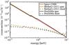 |
Fig. A.1 Comparison of X-ray photoelectric (absorption) cross-sections per hydrogen nucleus as a function of photon energy. The red line shows the gas absorption cross-section from Igea & Glassgold (1999). The brown lines show the cross-sections derived by Bethell & Bergin (2011). The black lines show the PRODIMO results for the large grains dust model. |
For the Igea & Glassgold (1999) cross-sections, we used their Eq. (10) for the case of heavy element depletion. Igea & Glassgold (1999) did not include a treatment of the absorption edges and also neglected the dust component. For the Bethell & Bergin (2011) cross-sections we used their Eq. (1) with the corresponding fitting coefficients for their “Gas” case (their Table 2); for the dust we used the coefficients for their dust size distribution with amin = 0.01 μm,amax = 1000 μm, and apow = 3.5 (their Table 3). We note that Bethell & Bergin (2011) did not use Mie-theory for the opacity calculations bur rather used directly the photo-electric cross-sections for the atoms and assumed that all heavy metals (except noble gases) and a certain fraction of C and O are in solid form. To account for different dust sizes they used self-blanketing factors.
The deviations between the Igea & Glassgold (1999) and PRODIMO cross-sections are on average ≈20% with a maximum of ≈30%. For the Bethell & Bergin (2011) cross-sections we find deviations of ≈10% with a maximum of ≈50%, relative to PRODIMO. The agreement for the gas cross-section is remarkably good considering that we did not adapt the exact same element abundances (although in all three cases some form of depleted abundances are use).
The Bethell & Bergin (2011) dust cross-sections are about a factor of 1.2−2 higher than the PRODIMO cross-sections. The differences are probably caused by the different dust properties (e.g. in the PRODIMO case amax = 3000 μm). However, considering the general uncertainties connected to X-ray dust opacities the agreement is quite good.
Appendix B: Comparison to the Monte Carlo X-ray radiative transfer code MOCASSIN
Ercolano & Glassgold (2013) presented a comparison of the 3D Monte Carlo radiative transfer and photoionization code MOCASSIN (Ercolano et al. 2008b) to the Monte Carlo X-ray radiative transfer model of Igea & Glassgold (1999). For the comparison a minimum mass solar nebula disk model is used (see Igea & Glassgold 1999 for details). The X-ray emitting source is modelled via two rings with radius 5 R⊙ located at a height of 5 R⊙ above and below the star. Dust absorption and scattering is not considered in those models. Ercolano & Glassgold (2013) found a good agreement for the resulting X-ray ionization rates per hydrogen nucleus between the two codes.
In Fig. B.1 we show a comparison of our X-ray radiative transfer model to the results from MOCASSIN. For this comparison we used the same physical disk parameters and the same initial element abundances (the “IG99 depleted”) as given in Ercolano & Glassgold (2013). The X-ray luminosity is LX(1−20 keV) = 1029 erg s-1 and the spectrum has a single temperature of kTX = 5 keV. In contrast to the models presented in Ercolano & Glassgold (2013) we assume that the X-rays are emitted at the stellar surface. The X-ray ionization rate ζX is simply calculated for the given initial abundances (i.e. all species are neutral and all hydrogen is in molecular form) without solving for the chemistry.
As seen from Fig. B.1, the agreement of the two codes is quite good but there are also some significant differences. We want to emphasize that the radiative transfer methods used are very different. MOCASSIN uses the Monte Carlo approach with a proper treatment of anisotropic scattering. In PRODIMO, we apply a ray-base method (discrete-ordinates) with a simple approximation for the anisotropic scattering. Scattering dominates ζX for NH,ver ≳ 1023 cm-2 (scattering shoulder Igea & Glassgold 1999). In this region the results of both codes are within a factor of three, indicating that our simplified treatment of anisotropic scattering is a reasonable approximation.
The largest differences are actually at low column densities of N⟨ H ⟩ ,ver ≲ 1021 cm-2 where ζX is solely dominated by absorption of low-energy X-ray photons (here EX ≈ 1 keV ). Those deviations might be caused by the exact treatment of the low-energy cut-off for the X-ray spectrum. We did run a test with a cut-off at 1.1 keV in that case ζX drops by a factor of a few at low column densities but is not affected at high column densities. However, we also performed a test with twice as much energy bands in our X-ray RT to more accurately treat the low-energy cut-off, but we did not find significant differences. So, the origin of these deviations remains rather unclear. Although ζX at low columns is relevant for photo-evaporative winds (e.g. Ercolano et al. 2008a) it is of less relevance for our here presented models as we are mainly interested in the impact of X-ray ionization on the chemistry.
The deviations around N⟨ H ⟩ ,ver = 1023 cm-2 are likely caused by the different locations of the X-ray emitting source. Compared to a pure stellar X-ray source, the X-ray photons emitted by an elevated ring source have encountered a lower column of material when they reach a certain height of the disk (see also Igea & Glassgold 1999). At larger distances the geometrical effects (e.g. incident angle on the disk surface) are less severe. The actual location of the X-ray source in T Tauri stars is not well known which is a general uncertainty in the models. However, as discussed by Ercolano et al. (2009) there are observational indications for a location of the X-ray source at or very close (≲1 R⊙) to the stellar surface.
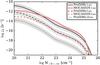 |
Fig. B.1 Comparison of the X-ray ionization rate ζX as a function of vertical hydrogen column density N⟨ H ⟩ ,ver at radii of 1 au (solid lines), 5 au (dashed lines) and 10 au (dotted line). The red lines are the results from MOCASSIN the black lines are the results from PRODIMO. The 10 au result from MOCASSIN were not available for this test case. The 10 au results have been scaled down by a factor of 10 for better visibility. The grey shaded area indicates a factor of three deviation relative to the PRODIMO results. An isothermal X-ray spectrum with kTX = 5 keV and LX = 1029 erg s-1 is used. |
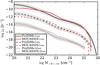 |
Fig. B.2 Same as Fig. B.1 but for a flared X-ray spectrum and low metal abundances. The 5 and 10 au results have been scaled down by factor of 10 and 1000, respectively. The X-ray luminosity is LX = 2 × 1031 erg s-1 and the plasma temperature is kTX = 12 keV (the COUP flared spectrum in Ercolano & Glassgold 2013). |
In Fig. B.2, we present a similar comparison as in Fig. B.1 but for a flared X-ray spectrum with LX(1−20 keV) = 2 × 1031 erg s-1 and kTX = 12 keV and different element abundances (“ISM depleted” from Table 1 of Ercolano & Glassgold 2013). The deviations between the models are similar to the first test case. However, now the impact of the X-ray source location is better visible. In the MOCASSIN models the scattering shoulder is located at slightly deeper layers than in the PRODIMO models. Due to the elevated location of the X-ray source the photons experience a lower radial column of material and can penetrate to deeper layers of the disk. The differences for N⟨ H ⟩ ,ver> 1025 cm-2 are likely of technical nature. As noted by Ercolano & Glassgold (2013) the sudden drop in ζX is caused by the low number of photons reaching those layers. In the PRODIMO model convergence of the iterative scheme might not be reached in the high-energy range where scattering is most important. This results in an overestimate of ζX in deep and dense regions of the disk. However, in such regions, ζX ≲ 10-19 s-1, which is below the ionization rates expected from cosmic rays and the decay of short-lived radionuclides (e.g. Umebayashi & Nakano 2009; Cleeves et al. 2015).
Although there are differences concerning the X-ray ionization rate between PRODIMO and MOCASSIN, the overall agreement is quite good. In particular, it shows that our ray-based radiative transfer method gives similar results as the Monte Carlo radiative transfer method. However, as the calculation of the X-ray ionization rate is a rather complex topic, a proper and more detailed benchmarking of different X-ray radiative transfer codes is desirable for a better understanding of the remaining model differences.
Appendix C: X-ray photoelectric cross-sections for PAHs
In Fig. C.1 we show the photo-electric (absorption) cross-section of PAHs (Polycyclic aromatic hydrocarbons) in comparison to the X-ray gas and dust cross-sections used in our reference model (i.e. large grains dust model; see Fig. 4). The PAH absorption cross-sections are from Li & Draine (2001)3. They provide absorption cross-sections for various PAH sizes in the X-ray energy domain up to 2 keV, assuming graphite-like optical properties. We used neutral PAH particles with 54 carbon and 18 hydrogen atoms and a radius of ≈4.87 × 10⁻⁴μm (the same PAH properties as are used for our chemical model) and considered an ISM like PAH abundance of ≈2.8 × 10⁻⁷ (Tielens 2008). Further details on the treatment of PAHs in our model can be found in Woitke et al. (2016).
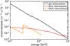 |
Fig. C.1 Comparison of PAH photoelectric (absorption) cross-sections per hydrogen nucleus in the X-ray regime to the dust and gas absorption cross-sections. |
It is clear from Fig. C.1 that, compared to the gas, PAHs play an insignificant role in the X-ray radiative transfer and for the disk X-ray radiation field. Furthermore, the PAH abundance in disks around T Tauri stars is likely significantly lower than in the ISM (e.g. Geers et al. 2006), which further reduces the importance of PAHs as an opacity source (similar to the far-UV wavelength regime, see Woitke et al. 2016). For all models presented in this paper, we assumed a PAH abundance reduced by a factor of 100 compared to the ISM. Nevertheless, X-rays might play an essential role for the destruction of PAHs in disks. Due to their high energies, X-ray photons can efficiently destroy PAHs on timescales significantly shorter than typical disk lifetimes (Siebenmorgen & Krügel 2010; Siebenmorgen & Heymann 2012). However, here we are mainly interested in the overall X-ray disk radiation field and the resulting X-ray ionization rates and therefore do not include PAHs in the X-ray radiative transfer.
Appendix D: HCO+ formation pathway via excited molecular hydrogen
The formation pathway for HCO+ via excited molecular hydrogen works in the following:
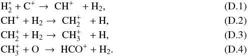 Key here is the reaction
 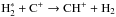 , where we use the measured rate of Hierl et al. (1997) with an extrapolation to lower temperatures. However, in particular the rate at low temperatures (T < 100 K) is uncertain, and theoretical models indicate significantly lower rates (by orders of magnitude, Zanchet et al. 2013). A more detailed discussion and a comparison of different rates for
  is presented in Kamp et al. (2017).
All Tables
All Figures
|
Fig. 1 Gas disk structure. Top panel: total hydrogen number density n⟨ H ⟩. The height of the disk z is scaled by the radius r. The white dashed contours correspond to the density levels shown in the colour bar. Bottom panel: total vertical hydrogen column number density N⟨ H ⟩ ,ver as a function of radius where on the right-hand side also the scale for the surface density Σ in g cm-2 is given. |
| In the text | |
|
Fig. 2 Large grains (left column) and small grains (right column) disk model. From top to bottom the dust density, dust temperature, gas temperature and the disk UV radiation field χ in units of the Draine field are shown. The dashed contours in each plot correspond to the levels shown in the respective colour bar. The additional contours in the UV plots (bottom row) indicate where the radial (red solid line) and vertical (black solid line) visual extinctions are equal to unity. For both models, the same gas density structure as shown in Fig. 1 is used. |
| In the text | |
|
Fig. 3 Optical constants (n,k) for astronomical silicates in the X-ray regime. n (top panel) is the real and k (bottom panel) the imaginary part of the complex refractive index. The red solid lines show the results from this work and the black solid lines show the results from Draine (2003). |
| In the text | |
|
Fig. 4 X-ray cross-sections for the gas (black lines) and dust (blue and red lines) per hydrogen nucleus for three different dust-size distributions. The solid lines show the extinction (absorption+scattering) cross section and the dashed lines are the scattering cross sections. The left panel is for the MRN size distribution (Mathis et al. 1977) using pure astronomical silicates (Draine 2003). The two other panels are for the small and large grains dust models (see Sect. 2.2.1). For the dust, the red lines are for isotropic and the blue lines for pseudo anisotropic (pa) scattering (see Sect. 2.3.2). The pseudo anisotropic scattering values (blue dashed lines) are multiplied by a factor of 1000. The shown gas cross-sections are the same in all three panels. |
| In the text | |
|
Fig. 5 X-ray background field spectra. The black solid line shows a cluster X-ray background field as proposed by Adams et al. (2012) with a flux of 2 × 10⁻⁵ erg cm-2 s-1 modelled with a bremsstrahlungs spectrum with TX = 2 × 10⁷K. The red and blue solid lines are for fluxes ten times higher and lower, respectively. For comparison we also show the diffuse extragalactic X-ray background field (XRB, brown solid line) using the fits described in Fabian & Barcons (1992) and a hot-gas spectrum (magenta line) from, for example, Supernova remnants (see Tielens 2005 chap. 1; Slavin & Frisch 2008). |
| In the text | |
|
Fig. 6 X-ray ionization rate ζX for the 2D disk structure. Top panel: model with only gas absorption. Bottom panel: model with gas absorption and scattering. The white solid contour line shows N⟨ H ⟩ ,rad = 2 × 1024 cm-2, which corresponds roughly to the X-ray scattering surface. Below this surface ζX starts to be dominated by scattered X-ray photons. The white and red dashed lines show N⟨ H ⟩ ,ver = 2 × 1022 cm-2 and N⟨ H ⟩ ,ver = 2 × 1024 cm-2, respectively. |
| In the text | |
|
Fig. 7 X-ray ionization rate ζX vs. vertical column density N⟨ H ⟩ ,ver at disk radii of 1 au (left panel) and 100 au (right panel), respectively. The dashed lines show models with X-ray gas opacities only, where the purple line is for pure absorption and the orange line for absorption plus scattering. The solid lines are for models including X-ray dust opacities (absorption+scattering), where results for the small grains (SG, blue), medium grains (MG, red) and large grains (LG, black) dust models are shown. The vertical grey line in both plots indicates the scattering surface at N⟨ H ⟩ ,rad = 2 × 1024 cm-2 (see also Fig. 6); at the right hand side of this line ζX is dominated by scattered high-energy photons. The horizontal lines mark the cosmic-ray ionization rates for the ISM (ζCR ≈ 10-17), and low cosmic-ray case (ζCR ≈ 10-19 s-1). |
| In the text | |
|
Fig. 8 X-ray ionization rate ζX for the three different dust models including X-ray opacities for the gas and the dust. The white solid contour shows N⟨ H ⟩ ,rad = 2 × 1024 cm-2, which corresponds to the scattering surface. The dashed white contour shows where ζX is equal to ζX,abs of the gas absorption only model. Above this line ζX ≤ ζX,abs (additional absorption by the dust) and below, ζX>ζX,abs (scattering). |
| In the text | |
|
Fig. 9 X-ray ionization rate ζX for a model with LX = 1029 erg s-1 and FXBGF = 2 × 10⁻⁵ erg cm-2 s-1 (i.e. the benchmark values of Adams et al. 2012). The white solid contour line encloses the region where the XBGF dominates ζX (i.e. ζX,XBGF ≥ ζX, ∗). |
| In the text | |
|
Fig. 10 X-ray ionization rate in the midplane (left panel) and for a vertical cut at r = 150 au (right panel) for models with fixed stellar X-ray luminosity (LX = 1030 erg s-1) but varying X-ray background fields with fluxes of 2 × 10⁻⁴ (blue), 2 × 10⁻⁵ (brown) and 2 × 10⁻⁴ erg cm-2 s-1 (red); the black lines are for the model without an XBGF. The solid lines are for the full X-ray spectra (0.1−20 keV); the dotted and dashed lines correspond to models with a low-energy cut-off at 0.3 keV and 1 keV, respectively. The horizontal lines mark the cosmic-ray ionization rates for the ISM (ζCR ≈ 10-17), and low cosmic-ray case (ζCR ≈ 10-19 s-1). In the right panel, the vertical grey solid line indicates the scattering surface at N⟨ H ⟩ ,rad = 2 × 1024 cm-2 (see also Fig. 7). |
| In the text | |
|
Fig. 11 HCO+ (left column) and N2H+ (right column) radial column density profiles for models with different dust-size distributions: small grains (SG, blue), medium grains (MG, red), and large grains (LG, black). The dashed lines are for models where only the gas component is considered in the X-ray RT, where the solid lines show models where both X-ray gas and dust opacities are included. The ISM cosmic-ray models are shown in the top row and the low cosmic-ray models are shown in the bottom row. The grey shaded area marks a difference of a factor three in N with respect to the reference model (LG gas+dust). |
| In the text | |
|
Fig. 12 Radial column density profiles for HCO+ and N2H+ with (coloured lines) and without (black lines) XBGF for the ISM (top row) and low (bottom row) cosmic-ray case. The dashed lines are for models with a low-energy cut-off of the X-ray spectra (stellar and XBGF) of 1 keV; for the solid lines the lowest X-ray energy is 0.1 keV. The grey shaded area marks a factor of three difference in N with respect to the models without XBGF (the solid black line). |
| In the text | |
|
Fig. A.1 Comparison of X-ray photoelectric (absorption) cross-sections per hydrogen nucleus as a function of photon energy. The red line shows the gas absorption cross-section from Igea & Glassgold (1999). The brown lines show the cross-sections derived by Bethell & Bergin (2011). The black lines show the PRODIMO results for the large grains dust model. |
| In the text | |
|
Fig. B.1 Comparison of the X-ray ionization rate ζX as a function of vertical hydrogen column density N⟨ H ⟩ ,ver at radii of 1 au (solid lines), 5 au (dashed lines) and 10 au (dotted line). The red lines are the results from MOCASSIN the black lines are the results from PRODIMO. The 10 au result from MOCASSIN were not available for this test case. The 10 au results have been scaled down by a factor of 10 for better visibility. The grey shaded area indicates a factor of three deviation relative to the PRODIMO results. An isothermal X-ray spectrum with kTX = 5 keV and LX = 1029 erg s-1 is used. |
| In the text | |
|
Fig. B.2 Same as Fig. B.1 but for a flared X-ray spectrum and low metal abundances. The 5 and 10 au results have been scaled down by factor of 10 and 1000, respectively. The X-ray luminosity is LX = 2 × 1031 erg s-1 and the plasma temperature is kTX = 12 keV (the COUP flared spectrum in Ercolano & Glassgold 2013). |
| In the text | |
|
Fig. C.1 Comparison of PAH photoelectric (absorption) cross-sections per hydrogen nucleus in the X-ray regime to the dust and gas absorption cross-sections. |
| In the text | |
Current usage metrics show cumulative count of Article Views (full-text article views including HTML views, PDF and ePub downloads, according to the available data) and Abstracts Views on Vision4Press platform.
Data correspond to usage on the plateform after 2015. The current usage metrics is available 48-96 hours after online publication and is updated daily on week days.
Initial download of the metrics may take a while.