| Issue |
A&A
Volume 606, October 2017
|
|
|---|---|---|
| Article Number | A29 | |
| Number of page(s) | 21 | |
| Section | Interstellar and circumstellar matter | |
| DOI | https://doi.org/10.1051/0004-6361/201730881 | |
| Published online | 03 October 2017 | |
[C II] emission from L1630 in the Orion B molecular cloud
1 Leiden Observatory, Leiden University, PO Box 9513, 2300 RA Leiden, Netherlands
e-mail: This email address is being protected from spambots. You need JavaScript enabled to view it.
2 ICMM-CSIC, Calle Sor Juana Ines de la Cruz 3, 28049 Cantoblanco, Madrid, Spain
3 Herschel Science Center, ESA/ESAC, PO Box 78, Villanueva de la Cañada, 28691 Madrid, Spain
4 CNRS, IRAP, 9 avenue Colonel Roche, BP 44346, 31028 Toulouse Cedex 4, France
5 Department of Physics and Astronomy, The Johns Hopkins University, 3400 North Charles Street, Baltimore, MD 21218, USA
6 Department of Astronomy, University of Maryland, College Park, MD 20742, USA
7 I. Physikalisches Institut der Universität zu Köln, Zülpicher Strasse 77, 50937 Köln, Germany
8 Max-Planck-Institut für Radioastronomie, Auf dem Hügel 69, 53121 Bonn, Germany
9 IRAM, 300 rue de la Piscine, 38406 Saint-Martin-d’Hères, France
10 LERMA, Observatoire de Paris, PSL Research University, CNRS, Sorbonne Universités, UPMC Univ. Paris 06, 75014 Paris, France
Received: 28 March 2017
Accepted: 9 June 2017
Abstract
Context. L1630 in the Orion B molecular cloud, which includes the iconic Horsehead Nebula, illuminated by the star system σ Ori, is an example of a photodissociation region (PDR). In PDRs, stellar radiation impinges on the surface of dense material, often a molecular cloud, thereby inducing a complex network of chemical reactions and physical processes.
Aims. Observations toward L1630 allow us to study the interplay between stellar radiation and a molecular cloud under relatively benign conditions, that is, intermediate densities and an intermediate UV radiation field. Contrary to the well-studied Orion Molecular Cloud 1 (OMC1), which hosts much harsher conditions, L1630 has little star formation. Our goal is to relate the [C ii] fine-structure line emission to the physical conditions predominant in L1630 and compare it to studies of OMC1.
Methods. The [C ii] 158 μm line emission of L1630 around the Horsehead Nebula, an area of 12′ × 17′, was observed using the upgraded German Receiver for Astronomy at Terahertz Frequencies (upGREAT) onboard the Stratospheric Observatory for Infrared Astronomy (SOFIA).
Results. Of the [C ii] emission from the mapped area 95%, 13 L⊙, originates from the molecular cloud; the adjacent H ii region contributes only 5%, that is, 1 L⊙. From comparison with other data (CO (1 − 0)-line emission, far-infrared (FIR) continuum studies, emission from polycyclic aromatic hydrocarbons (PAHs)), we infer a gas density of the molecular cloud of nH ~ 3 × 103 cm-3, with surface layers, including the Horsehead Nebula, having a density of up to nH ~ 4 × 104 cm-3. The temperature of the surface gas is T ~ 100 K. The average [C ii] cooling efficiency within the molecular cloud is 1.3 × 10⁻². The fraction of the mass of the molecular cloud within the studied area that is traced by [C ii] is only 8%. Our PDR models are able to reproduce the FIR-[C ii] correlations and also the CO (1 − 0)-[C ii] correlations. Finally, we compare our results on the heating efficiency of the gas with theoretical studies of photoelectric heating by PAHs, clusters of PAHs, and very small grains, and find the heating efficiency to be lower than theoretically predicted, a continuation of the trend set by other observations.
Conclusions. In L1630 only a small fraction of the gas mass is traced by [C ii]. Most of the [C ii] emission in the mapped area stems from PDR surfaces. The layered edge-on structure of the molecular cloud and limitations in spatial resolution put constraints on our ability to relate different tracers to each other and to the physical conditions. From our study, we conclude that the relation between [C ii] emission and physical conditions is likely to be more complicated than often assumed. The theoretical heating efficiency is higher than the one we calculate from the observed [C ii] emission in the L1630 molecular cloud.
Key words: ISM: clouds / ISM: structure / H ii regions / galaxies: ISM / infrared: ISM
© ESO, 2017
1. Introduction
One of the main challenges of astronomy and cosmology is to model, and reach an understanding, of the evolution of galaxies and large-scale structure. The star-formation rate (SFR) is a crucial parameter in these models. In order to measure the SFR in distant galaxies, several possible tracers have been and are being studied: ultraviolet (UV) radiation, infrared (IR) radiation, emission from polycyclic aromatic hydrocarbons (PAHs), atomic and molecular lines (e.g., Kennicutt 1998; Kennicutt & Evans 2012). With the advent of the Atacama Large (sub)Millimeter Array (ALMA), it has become popular to use the [C ii] 158 μm line as an indicator of the SFR over cosmic history (e.g., Herrera-Camus et al. 2015; Vallini et al. 2015; Pentericci et al. 2016). However, the origin of [C ii] emission on a galactic scale is still unclear.
Intuitively, the SFR is expected to depend on the local conditions in the interstellar medium (ISM), the gas and dust that form the environment of stars. The ISM comes in different phases, diffuse gas being the most prevalent. These phases are the cold neutral medium (CNM) with moderate gas densities, n ~ 30 cm-3, and moderate gas temperatures, T ~ 100 K, the warm neutral and warm ionized medium (WNM and WIM) with low densities and high temperatures, n ~ 0.3 cm-3 and T ~ 8000 K, and the hot ionized medium (HIM) with very low densities and very high temperatures, n ~ 3 × 10⁻³ cm-3 and T ~ 106 K. Most of the gas of the ISM is in the neutral phase. Other ubiquitous components of the ISM are H ii regions around massive stars with densities ranging from n ~ 1 cm-3 to n ~ 105 cm-3 and T ~ 104 K, and molecular clouds with high density and low temperatures, n ~ 103 − 108 cm-3 and T ~ 10 − 30 K (Hollenbach & Tielens 1999). These phases are not isolated from each other, but there is an exchange of matter between them, particularly driven by ionization, winds, and explosions of massive stars. Molecular clouds especially are the birthplaces of new (massive) stars and thereby of vital interest. Meyer et al. (2008) provide a review of star formation in L1630. At the interface between an H ii region, ionized by a massive star, and a parental molecular cloud, a photodissociation region (PDR) is formed, where intense stellar UV radiation impinges on the surface of the dense cloud. At the surface of these clouds, the gas is atomic; deeper inside the cloud, the molecular fraction increases. The study of PDRs reveals much about the interplay between stars (including hosts of newly formed stars) and the ISM, thereby yielding valuable insight into the process of star formation (see Hollenbach & Tielens 1999, for a review of PDRs).
The ISM is mainly heated by stellar radiation, specifically by far-ultraviolet (FUV) radiation with energies between 6 and 13.6 eV. The characteristics of the gas cooling allow us to infer the amount and, possibly, the source of the heating. One of the main coolants of the cold neutral medium is the [C ii]  fine-structure line at λ ≃ 158 μm, that is, ΔE/kB ≃ 91.2 K. The [C ii] line is also one of the brightest lines in PDRs, carrying up to 5% of the total far-infrared (FIR) luminosity, the other 95% mainly stemming from UV irradiated dust. Carbon has an ionization potential of 11.3 eV, hence C+ traces the transition from H+ to H and H2. Another important coolant is the [O i] line at λ ≃ 63 μm (ΔE/kB ≃ 228 K). The ratio of those two main coolants depends on the temperature and density of the gas. For T = 100 K, the [O i] cooling efficiency overtakes the [C ii] cooling efficiency at n ≃ 3 × 104 cm-3; at n = 3 × 103 cm-3, the [O i] contribution to the total cooling is about 5% (cf. Tielens 2010).
The [C ii] line has been studied in a variety of environments. Important contributions may come from diffuse clouds (CNM), dense PDRs, surfaces of molecular clouds, and (low-density) ionized gas including the WIM (e.g., Wolfire et al. 1995; Ossenkopf et al. 2013; Gerin et al. 2015). Langer et al. (2010) identify warm CO-dark molecular gas in Galactic diffuse clouds by means of [C ii] emission. Jaffe et al. (1994) conducted an earlier study observing the extended [C ii] emission from the Orion B molecular cloud (L1630). This study is preceded by a [C ii] survey of the Orion Molecular Cloud 1 (OMC1) in Orion A by Stacey et al. (1989). Goicoechea et al. (2015) present a velocity-resolved [C ii] map toward OMC1, observed by the Heterodyne Instrument for the Far-Infrared (HIFI) onboard the Herschel satellite in 2012. Velocity-resolved [C ii] and [13C ii] emission from the star-forming region NGC 2024 in L1630 was observed in 2011 using the GREAT (German Receiver for Astronomy at Terahertz Frequencies) instrument onboard the airborne Stratospheric Observatory for Infrared Astronomy (SOFIA) and analyzed by Graf et al. (2012); the neighboring reflection nebula NGC 2023 was observed in 2013/14 using the same instrument. Sandell et al. (2015) discussed the physical conditions, morphology, and kinematics of that region. A theoretical study on collisional excitation of the [C ii] fine-structure transition was performed by Goldsmith et al. (2012). The GOT C+ survey (Galactic Observations of Terahertz C+) survey (Pineda et al. 2014), also a Herschel/HIFI study, investigated specifically the relationship between [C ii] luminosity and SFR. This study found a good correlation on Galactic scales. This was also established by Stacey et al. (2010) and Herrera-Camus et al. (2015) at low and high redshift.
On December 11, 2015, a part of the Orion B molecular cloud, including the Horsehead Nebula, was observed in [C ii] with the upGREAT instrument, the first multi-pixel extension of GREAT, onboard SOFIA, as presented and described in Risacher et al. (2016). The survey was conducted “to demonstrate the unique and important scientific capabilities of SOFIA, and to provide a publicly available high-value SOFIA data set”1. It allows us to study [C ii] emission and its correlations with other astrophysical tracers under moderate conditions (intermediate density and moderate UV-radiation field), as opposed to the high density and intense UV-radiation field in OMC1.
In the present study, we analyze the [C ii] emission from a 12′ × 17′ area of the L1630 molecular cloud in Orion B that is illuminated by the nearby star system, σ Ori. Our distance to the star system is approximately 334 pc, which we also assume to be the distance to the molecular cloud. The projected distance between the star system and the molecular cloud is 3.2 pc (Ochsendorf et al. 2014, and references therein). Part of the mapped area, in which star formation is low, is the well-known Horsehead Nebula. The star-forming regions NGC 2023 and NGC 2024 are adjacent to the mapped area, but not included. We compare the velocity-resolved [C ii] SOFIA/upGREAT observations with new CO (1 − 0) observations of the molecular gas obtained with the 30 m telescope (Pety et al. 2017) at the Institut de Radioastronomie Millimétrique (IRAM), with Spitzer/Infrared Array Camera (IRAC) studies of the PAH emission from the PDR surfaces, Hα observations of the ionized gas, and with existing far-infrared continuum studies using Herschel/Photoconductor Array Camera and Spectrometer (PACS) and Spectral and Photometric Imaging Receiver (SPIRE) data to determine dust properties and trace the radiation field. This wealth of data allows us to separate emission from the ionized gas, neutral PDR, and molecular cloud, in order to derive global heating efficiencies and their dependence on the local conditions, and to make detailed comparisons to PDR models.
This paper is organized as follows. In Sect. 2, we present the observations. In Sect. 3, we divide the surveyed area into regions with specific characteristics. Furthermore, we study the kinematics of the gas as revealed by the SOFIA/upGREAT observations of [C ii] emission and the correlation of the various data sets with each other. Section 4 contains a discussion of the results obtained in Sect. 3 and we derive column densities and other gas properties. We conclude with a summary of our results and an outlook for the future in Sect. 5.
2. Observations
2.1. [C II] observations
The [C ii] emission in Orion B (L1630) was observed on December 11, 2015 using the upGREAT instrument onboard SOFIA. The region was observed using the upGREAT optimized on-the-fly mapping mode. The region was split into four tiles, each covering an area of 363″ × 508.2″. In this mode, the array is rotated 19.1° on the sky and an on-the-fly (OTF) scan is undertaken. By performing a second scan separated by 5.5″ perpendicular to the scan direction, it is possible to fully sample a region 72.6″ wide along the scan direction (cf. Risacher et al. 2016, for details). By combining OTF scans in the RA and Dec direction, it is possible to cover the map region with multiple pixels. Each tile was made up of 10 x-direction OTF scans and 14 y-direction OTF scans. A spectrum was recorded every 6″. Scans in the x-direction had an integration time of 0.4 s, while those in the y-direction had an integration time of 0.3 s. Since the y-scan length is longer than the x-scan length, the integration time was reduced. This is due to Allan variance stability time limits of 30 s. A reference position at about 12′ to the west of the map was observed, which was verified to be free of 12CO (2 − 1) and 13CO (2 − 1) emission with the James Clerk Maxwell Telescope (JCMT; G. Sandell, priv. comm.). The reference position was checked to be free of [C ii] emission to a 1 K level. A supplementary off contamination check was undertaken whereby the reference position was calibrated using the internal hot reference measurement; these spectra also showed no evidence of off emission to a 1 K level. The [C ii] map itself, showing no “absorption” features anywhere, confirms that there cannot be notable [C ii] emission at the reference position. An off measurement is ideally taken after 30 s of on source integration to avoid drift problems in the calibrated data. For this observing run, each tile was observed twice in the x- and y-directions, resulting in a total integration time per map pixel of 1.4 s. For a spectral resolution of 0.19 km s-1, this results in a noise rms in the final data cube of 2 K in the velocity channels free of emission.
The data cube provided by the SOFIA Science Center was processed using the Grenoble Image and Line Data Analysis Software2/Continuum and Line Analysis Single-dish Software (GILDAS/CLASS). We subtract a baseline of order one from the spectra. The spectral data were integrated over the velocity range (with respect to the local standard of rest, LSR) vLSR = 6 − 20 km s-1 to obtain the line-integrated intensity, which is shown in Fig. 1. Channel maps are shown in Fig. 4. The spatial resolution of our final maps is 15.9″. For comparison with other tracers, we use a Gaussian kernel for convolution. At the rim of the map, the [C ii] signal suffers from noise and we ignore an outer rim of 45″ in our analysis.
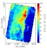 |
Fig. 1 [C ii] line-integrated intensity; points indicate positions where individual spectra are extracted for illustrative purposes (see Sect. 3.3). |
2.2. Dust SED analysis
In this study we make use of the dust temperature and dust optical depth maps released by Lombardi et al. (2014). Lombardi et al. (2014) fit a spectral energy distribution (SED) to Herschel/PACS and SPIRE observations of the Orion molecular cloud complex in the PACS 100 μm and 160 μm, and SPIRE 250 μm, 350 μm, and 500 μm bands. The photometric data, convolved to the SPIRE 500 μm36″ resolution, are modeled as a modified blackbody,  (1)with Td the effective dust temperature, τ0 the dust optical depth at the reference wavelength λ0, and β the grain-emissivity index. Lombardi et al. (2014) use the all-sky β map with 35′ resolution by the Planck collaboration, interpolated to the grid on which the SED is performed; only the effective dust temperature and τ0 are free parameters in this fit. The β map shows a smooth increase of about 3% from the north-east to the south-west in the area surveyed in [C ii], with a mean of 1.56. Lombardi et al. present their dust optical depth map at λ0 = 850 μm, following the Planck standard, but for our analysis we convert τ850 to τ160 using the β data. We integrate Eq. (1) from λmin = 20 μm to λmax = 1000 μm to obtain the far-infrared intensity IFIR.
We notice that the Horsehead PDR has comparatively low dust temperature in the SED fit, Td ≃ 20 − 22 K. This could be due to beam dilution. In the models of Habart et al. (2005), the dust temperature is Td ≃ 30 K at the edge, dropping to Td ≃ 22 K for a hydrogen nucleus gas density of nH = 2 × 104 cm-3 within 12″, and to Td ≃ 13.5 K for nH = 2 × 105 cm-3. Throughout this paper, by “gas density” we mean the hydrogen nucleus gas density: nH = nH i + 2 nH2.
The derived effective dust temperature and dust optical depth can depend significantly on the choice of β: the temperature can be up to 3 − 4 K lower if β = 2 instead of β = 1.5; τ160 then increases by a factor of two. The FIR intensity is less sensitive to β: it only decreases by 10% for β = 2.
Furthermore, we employ Spitzer/IRAC observations in the 8 μm band, which is dominated by PAHs but which can be influenced by very small grains. We use a super mosaic image retrieved from the Spitzer Heritage Archive, created October 22, 2012. We also make use of the 850 μm observations from the Submillimetre Common-User Bolometer Array 2 (SCUBA-2) around NGC 2023/2024 first presented by Kirk et al. (2016) as part of the JCMT Gould Belt Survey (GBS). These trace dense regions within the molecular cloud. However, we do not use the map reduced by the GBS group, but we retrieved the data from the Canadian Astronomy Data Centre (CADC) archive, processed on October 1, 2015.
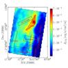 |
Fig. 2 [C ii] line-integrated intensity convolved to 36″ resolution with selected regions (see Sect. 3.2) indicated. |
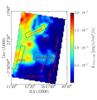 |
Fig. 3 CO (1 − 0) line-integrated intensity convolved to 36″ resolution with selected regions (see Sect. 3.2) indicated. |
2.3. CO (1–0) observations
In this work we make use of part of the 12CO (1 − 0) large-scale map at 115.271 GHz obtained by Pety et al. (2017) with the Eight Mixer Receiver (EMIR) 090 at the IRAM 30 m telescope. The fully sampled on-the-fly line maps were taken with a channel spacing of 195 kHz (a velocity resolution of ~0.5 km s-1). CO-emission contamination from the reference position was eliminated by adding dedicated frequency-switched line observations of the reference position itself (see Pety et al. 2017, for details). The median noise levels range from 100 to 180 mK (in the Tmb scale) per resolution channel. Here we use the CO (1 − 0) line-integrated intensity map in the vLSR = 9 − 16 km s-1 range3, convolved to the 36″ angular resolution of SPIRE 500 μm. The resulting map is shown in Fig. 3.
2.4. Hα observations
In this study we use the Hα image of the Horsehead Nebula and its environs in L1630 and the H ii region IC 434 taken by the Mosaic 1 wide field imager on Kitt Peak National Observatory (KPNO). For calibration of the KPNO image, we use Hα data of the Horsehead Nebula collected by the Hubble Space Telescope as part of the Hubble Heritage program. We obtained the image from the archive of the National Optical Astronomy Observatory (NOAO), but it was taken as part of the program presented in Reipurth et al. (1998).
The bright star at 05h41′02.70″, − 02°18′17.77″ in the Hα image is a foreground star; it is visible in the IRAC 8 μm image, as well. We masked it before convolution, such that it does not show in the convolved images.
3. Analysis
3.1. Kinematics: velocity channel maps
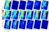 |
Fig. 4 [C ii] channel maps from 8.0 km s-1 to 16.0 km s-1 in steps of dv = 0.5 km s-1 at 15.9″ resolution. The main-beam temperature Tmb is averaged over the step size dv. The first panel shows the line-integrated intensity. |
Perusing the [C ii] channel maps from 8.0 km s-1 to 16.0 km s-1 shown in Fig. 4, we recognize several continuous structures in space-velocity. From 10.5 − 11.5 km s-1, we observe a [C ii] front that runs from the south-east to the north-west of the map. From 12.5 − 14.0 km s-1, a front runs from the north to the south. The Horsehead mane is visible from 10.0 − 11.5 km s-1. From 12.5 − 13.0 km s-1, an intermediate [C ii] front lights up. Based on the kinematic behavior and assuming that [C ii] emission is related to PDR surfaces, we divide the [C ii] fronts into four groups: PDR1 in the north-west of the molecular cloud, PDR2 in the south-west, PDR3 in the south-east, and the Horsehead PDR. The intermediate PDR front we do not discuss in detail.
In the luminous north, an almost circular cavity forms in the center of the region of highest intensity. Its boundary lights up in the 14.0 km s-1 map. In the 12.5 km s-1 and 13.0 km s-1 channels, we see bright emission where the rim of the cavity is. This cavity appears quite clearly in the unconvolved IRAC 8 μm image (see Fig. 15). Comparison with the 8 μm map reveals a (proto-)star at the northern edge of the bubble. This star is visible in the Hα image as well, but it is not identified as a pre-main-sequence (PMS) object in Mookerjea et al. (2009). Here it is listed as MIR-29, a more evolved star in the vicinity of NGC 2023, identified by the Two Micron All Sky Survey (2MASS). In addition to the main emission in the velocity range vLSR = 6 − 20 km s-1, we see a faint [C ii] component at vLSR ≃ 5 km s-1, that has also been detected in CO observations by Pety et al. (2017). Due to its faintness, however, we will ignore it in our analysis.
3.2. Global morphology
Apart from the four PDR surfaces discussed in Sect. 3.1, we singled out other specific regions that stand out in their morphology in the respective quantities [C ii], CO, and IRAC 8 μm emission (see Fig. 5). The 8 μm emission is a tracer of UV-pumped polycyclic aromatic hydrocarbons (PAHs) and therefore of PDR surfaces. Ionized gas is traced by Hα emission, and CO traces the molecular hydrogen gas. The regions are indicated in Figs. 2 ([C ii] map) and 3 (CO (1 − 0) map). We outline the boundary between the H ii region IC 434 and the molecular cloud L1630 by the onset of significant [C ii] emission at the molecular cloud surface where we also have been guided by the Hα contour of highest emission (see Fig. 18).
The four PDR regions, among them the Horsehead PDR4, are distinct in the IRAC 8 μm map. The Horsehead PDR is not the most luminous part of the region in all maps. The brightest part is region PDR1. We define the neck of the Horsehead Nebula that is traced by the CO (1 − 0) line; in itself, it has little [C ii] emission, but part of it is covered by the [C ii]-emitting molecular cloud. Another part of the cloud, where there is little CO emission, we call CO-dark cloud. Deeper inside the molecular cloud, CO emission is high and we define a region of CO cores or clumps. The Horsehead PDR is likely to suffer from beam dilution in all images, since its scale length is found to be less than 10″ (Habart et al. 2005), which is smaller than the beam sizes in question. To the north-east of the map, we recognize the reflection nebula NGC 2023, which has been studied with SOFIA/GREAT in [C ii] emission by Sandell et al. (2015). This region will not be discussed here.
 |
Fig. 5 Different quantities with [C ii] emission in units of K km s-1 in contours: IFIR tracing the UV radiation field re-radiated in the FIR by dust particles, I8 μm tracing the UV radiation field by fluorescence of PAHs, ICO (1 − 0) tracing the molecular gas, τ160 tracing the dust column, IHα emitted by ionized gas, and, finally, the ratio I[ C ii ]/IFIR. All maps are convolved to 36″ spatial resolution and re-gridded to a pixel size of 14″, that of the SPIRE 500 μm map. |
Figure 5a shows the FIR intensity with [C ii] contours in the mapped area. The FIR intensity peaks close to [C ii] in the most luminous part (PDR1), but slightly deeper into the cloud. The Horsehead mane is bright in both [C ii] and FIR; the emission overlaps very well. PDR2 is more pronounced in [C ii] emission than in the FIR. PDR3 can only be surmised in IFIR, but it cannot be distinguished very clearly in the integrated [C ii] map either.
In Fig. 5b, we compare the 8 μm emission with [C ii] in contours. The 8 μm emission behaves in a similar way as IFIR, but structures stand out more decidedly. The 8 μm emission, too, peaks slightly deeper into the cloud than [C ii]. The bright regions in the Horsehead mane overlap; in both maps it is a thin filament. PDR2 is more pronounced in [C ii], but is distinguishable in I8 μm as well. PDR3 is more distinct in I8 μm.
The CO (1 − 0) emission in the mapped area does not resemble the pattern of [C ii] emission (Fig. 5c). In CO, the entire Horsehead and its neck light up with nearly equal intensity while the surroundings remain dark. PDR1 and 2 are not very bright in CO. Interestingly, there is a CO spot in PDR1, right where the cavity is observed in (unconvolved) [C ii] and 8 μm emission (see Figs. 4 and 15, respectively). A “finger” of CO emission, the “CO clumps”, points towards PDR1. PDR3 can be inferred as shadow in CO emission, that is, a ridge of low CO emission.
The τ160 map (Fig. 5d) resembles the CO (1 − 0) map. The Horsehead and its neck have higher dust optical depth than their surroundings; the material directly behind the mane is a peak in τ160, that overlaps partially with the [C ii] peak, but it peaks slightly deeper into the Horsehead. The [C ii] peak in PDR1 does not correspond to a peak in dust optical depth, although the onset of the molecular cloud is traced by an increase in τ160. PDR3 corresponds to an optically thin region compared to its environment. The region of highest dust optical depth at the eastern border of the map (not containing NGC 2023) corresponds to a region with little [C ii] emission, but high CO emission. The CO “finger” relates to enhanced dust optical depth.
PDR1 and PDR2 border on the H ii region, as can be seen from Fig. 5e. PDR2 overlaps with a region of significant Hα emission, tracing the ionized gas at the surface of the molecular cloud. The Hα map and the logarithmic [C ii] cooling efficiency I[ C ii ]/IFIR map (Fig. 5f) resemble each other. High [C ii] over FIR intensity ratios are found near the boundary with high Hα emission. However, I[ C ii ]/IFIR is a misleading measure in the H ii region, since IFIR does not trace the radiation field well here and I[ C ii ] is sufficiently low to be significantly affected by noise. Variations in I[ C ii ]/IFIR across the map span a range from 3 × 10⁻³ up to 3 × 10⁻². Table 1 lists the mean values of the [C ii] cooling efficiency η = I[ C ii ]/IFIR, [C ii] intensity I[ C ii ], CO(1 − 0) intensity I[ C0 (1 − 0) ], FIR intensity IFIR, and dust optical depth τ160 for the several regions defined above.
Mean values (standard deviation between brackets) of several quantities in the several regions (η = I[ C ii ]/IFIR).
3.3. Kinematics: velocity-resolved line spectra
Figure 6 displays spectra extracted towards different positions in the map, as indicated in Fig. 1. The positions are chosen as representative single points for the different regions we identified earlier. Details on the spectra, that is, peak position, peak temperature, and line width, are given in Table 2. Point A represents the Horsehead mane, B lies in the most luminous part of the map, C just north of it, whereas D is displaced to the east; all three represent PDR1. We chose additional points in PDR1, because B might be affected by the bubble structure discussed later. Point E lies in PDR2 behind the Horsehead and F in the southern part of PDR2. Point G is located in the intermediate PDR front which we do not discuss in detail. Point I represents PDR3, whereas H is chosen in the CO-dark cloud, where there is little [C ii] emission (and little emission in other tracers).
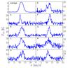 |
Fig. 6 Line spectra towards points A–I with average spectrum over the entire map (including H ii region) in the top left panel. Point A corresponds to the Horsehead PDR, points B to D are located in PDR1, points E and F lie in PDR2, point G represents the intermediate PDR front, point H is located in a region of little [C ii] emission, and point I represents PDR3. |
Results from Gaussian fit (points B–E with two components) to individual spectra with a spatial resolution of 15.9″ sampled at 7.55″.
The spectrum taken towards the Horsehead PDR (point A) shows a narrow line. Opposed to this is the line width of the spectrum extracted towards the most luminous part of the molecular cloud, point B: here, the line is broadened. It peaks at a slightly higher velocity than the Horsehead PDR. From comparison with the dust optical depth, we conclude that the broadening of the line is not due to a high column density (if dust density and gas density are related). The same holds for point C in PDR1. Here there appears a small side peak at higher velocity, which could also be inferred for point B (as a shoulder). Point D evidently has a spectrum with two peaks. From the distinctly different morphology of the channel maps at the two peak velocities (cf. Fig. 4 at 10.5 km s-1 and 13.0 km s-1), we surmise that the two peaks correspond to two distinct emitting components, rather than to one emission component with foreground absorption. The same goes for point E in PDR2, which also has two peaks. The southern part of PDR2, point F, has only one rather narrow peak. The intermediate PDR, point G, exhibits a strong narrow line, as well. The spectrum taken in the western PDR, point I, shows a somewhat broader line with somewhat lower intensity. At point H, where the intensity is low in all tracers, the [C ii] line is also broader.
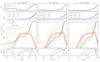 |
Fig. 7 Results of our edge-on models described in Sect. 3.4. The panels show the gas temperature T (upper panels), IFIR, I[ C ii ], I[ C ii ]/IFIR, and ICO (1 − 0) (middle panels) and C+, C, and CO fractional abundances (lower panels) versus physical scale, for the gas densities nH = 3.0 × 103 cm-3,1.6 × 104 cm-3,4.0 × 104 cm-3 (left to right panels), and AV,los = 0.5, 2.5, and5.0. We note that the gas temperature does not vary with AV,los. |
Strikingly, the peak velocity of point D is shifted towards lower velocity by 1 km s-1 with respect to points B and C (all PDR1). However, one component of this spectrum lies at about 11 km s-1, which is also the velocity of PDR3 (point I). This is further evidence that PDR3 and a part of PDR1 are spatially connected, as concluded from the channel maps. Point D in PDR1 has a component at about 13 km s-1, which is the velocity of PDR2. In B and C (PDR1) this component might be hidden beneath the strong side peak at 14 km s-1. The affiliation of the second component at point E in PDR2 is unclear; there might be another layer of gas behind or in front of the main component, or it could originate from the gas of PDR1 and PDR3 at 11 km s-1.
3.4. Edge-on PDR models
We supplement the correlation plots in the following section with model runs that are based on the PDR models of Tielens & Hollenbach (1985), with updates like those found in Wolfire et al. (2010) and Hollenbach et al. (2012). We include the most recent computations on fine-structure excitations of C+ by collisions with H by Barinovs et al. (2005) and with H2 by Wiesenfeld & Goldsmith (2014), and adopt a fractional gas-phase carbon abundance of 1.6 × 10⁻⁴ (Sofia et al. 2004). The line intensities are calculated for an edge-on case by storing the run of level populations with molecular cloud depth for the excited level of CO and C+ as calculated in the face-on model. For each line of sight, the intensity is found from integrating Eq. (B.14) in Tielens & Hollenbach (1985) through the layer of length z = NH/nH with the gas column density NH and the gas density nH, where we replace the factor (2π)-1 for a semi-infinite slab with (4π)-1. The cooling rate is given by Eq. (B.1) in Tielens & Hollenbach (1985) in the limit of no background radiation. For the escape probability we take the line-of-sight formulation  (2)where τ is the line optical depth calculated as in Eq. (B.8) in Tielens & Hollenbach (1985).
The FIR continuum intensity in the edge-on case is calculated from the run of dust temperature with depth into the molecular cloud. We find the dust temperature, Td, from the prescription given in Hollenbach et al. (1991). We integrate the dust absorption efficiency, Qabs, through the layer of length z (3)where we take the grain size a = 0.1 μm, and nd/nH = 6.36 × 10⁻¹², which gives a grain cross section per hydrogen atom of 2.0 × 10⁻²¹ cm2. For Qabs we use the average silicate and graphite value Qabs = 1.0 × 10⁻⁶(a/ 0.1 μm)(Td/ K)2 from Draine (2011).
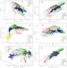 |
Fig. 8 Correlation plots extracted from the Orion B maps, convolved to a uniform resolution of 36″ and pixel size of 15″. Dark blue diamonds represent the CO-dark cloud, blue diamonds represent the CO clumps, red squares represent the Horsehead neck, triangles in different shades of green represent the PDRs (bright green is the Horsehead PDR), and yellow triangles represent the H ii region. Edge-on model predictions for selected gas densities are plotted as lines. Dashed lines are for AV,los = 2.5, with dark gray corresponding to a gas density of nH = 3.0 × 103 cm-3, medium gray to nH = 1.6 × 104 cm-3, and light gray to nH = 4.0 × 104 cm-3; dotted lines are the same but for AV,los = 5.0; the medium and light gray dash-dotted lines are for AV,los = 0.5, with nH = 1.6 × 104 cm-3 and nH = 4.0 × 104 cm-3, respectively. In panel f, the best fit is plotted as a line. |
In Fig. 7, we present the results of the models with an incident FUV intensity of G0 = 100 appropriate for σ Ori (Abergel et al. 2003 and references therein) and a Doppler line width of Δv = 1.5 km s-1 for different densities on a physical scale. The x-axes share the same range of visual extinction, AV = 0.0 − 9.3. We computed models for gas densities nH = 3.0 × 103 cm-3,1.6 × 104 cm-3, and 4.0 × 104 cm-3; those densities we estimate from the line cuts in Sect. 4.7 for different parts of the molecular cloud. We integrate along a length AV,los of the line of sight estimated in Sect. 4.4 for each density, where we assumed NH = 2.0 × 1021 cm-2AV. AV,los = 2.5and5.0 with nH = 3.0 × 103 cm-3 correspond to PDR1 and PDR2, respectively; AV,los = 0.5and2.5 with nH = 1.6 × 104 cm-3and4.0 × 104 cm-3 correspond to potentially dense cloud surfaces in PDR1 and PDR2. The Horsehead PDR should be matched with AV,los = 2.5or5.0 with nH = 4.0 × 104 cm-3.
The three models substantially show the same result, with a luke-warm surface layer where the gas cools through the [C ii] line. The colder gas deeper in the cloud emits mainly through CO. Not surprisingly, the FIR dust emission also peaks at the surface. The line-of-sight depth of the molecular cloud (AV,los = 0.5,2.5,or5.0) only slightly affects the ratios of FIR, [C ii]-, and CO-line intensities.
3.5. Correlation diagrams
Figure 8 shows correlation diagrams between several quantities. The different colors indicate the selected regions assigned in Sect. 3.2 and shown in Figs. 1 and 3. Gray points represent points that do not lie in either of the defined regions.
Figure 8a shows that the [C ii] cooling efficiency I[ C ii ]/IFIR decreases with increasing IFIR. The different PDRs lie on distinct curves, with similar slopes. Figure 8b shows increasing I[ C ii ] with increasing IFIR, but again in distinct branches for the different regions. The relation between I[ C ii ] and I8 μm resembles that, as can be seen from Fig. 8f, but simple fits reveal a tighter relation of I[ C ii ] with I8 μm than with IFIR. Over-plotted is a least-square fit ![Mathematical equation: \hbox{$I_{\mathrm{[C\,\textsc{ii}]}} \simeq 2.2\times 10^{-2} I_{8\,\mu\mathrm{m}}^{0.79}$}](/articles/aa/full_html/2017/10/aa30881-17/aa30881-17-eq230.png) (ρ = 0.85).
(ρ = 0.85).
As Fig. 8c shows, I[ C ii ] is roughly constant for higher τ160, that is, in PDR3 and the Horsehead PDR. This might reflect the fact that there is colder, non-PDR material located behind the PDR surfaces. PDR1 and PDR2 at the onset of the molecular cloud, where we do not expect a huge amount of colder material along the line of sight, show a nice correlation: PDR1 lies at twice as high τ160 and has twice as high I[ C ii ]. For small τ160 (i.e., in the H ii region and parts of the CO-dark cloud), the data show a steep rising slope. In Fig. 8d, there is no obvious relation between I[ C ii ]/IFIR and the dust temperature Td. Figure 8e shows I[ C ii ] versus ICO (1 − 0). Here we notice that the various regions populate distinct areas in the plot. In the diagram of I[ C ii ]/IFIR versus ICO (1 − 0)/IFIR (Fig. 9), we observe no obvious correlation, only the Horsehead PDR exhibits a significant slope.
The relation between I[ C ii ] and I8 μm resembles the relation of I[ C ii ] with IFIR, as can be seen from Fig. 8f, but simple fits reveal a tighter relation of I[ C ii ] with I8 μm than with IFIR. Over-plotted is a least-square fit, I[ C ii ] ≃ 2.2 × 10⁻² (I8 μm [ erg s-1 cm-2 sr-1 ] )0.79 erg s-1 cm-2 sr-1 (ρ = 0.85).
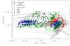 |
Fig. 9 Correlation plot of I[ C ii ]/IFIR versus ICO (1 − 0)/IFIR. Edge-on model predictions for selected gas densities are plotted as lines. Dashed lines are for AV,los = 2.5, with dark gray corresponding to a gas density of nH = 3.0 × 103 cm-3, medium gray to nH = 1.6 × 104 cm-3, and light gray to nH = 4.0 × 104 cm-3; dotted lines are the same but for AV,los = 5.0; the medium and light gray dash-dotted lines are for AV,los = 0.5, with nH = 1.6 × 104 cm-3 and nH = 4.0 × 104 cm-3, respectively. |
 |
Fig. 10 Correlation plot of I[ C ii ]/IFIR versus τ160. The plotted line corresponds to the relation expected from a simple face-on slab model, C/ (1 − exp( − τ160)); it is drawn such that it runs through the mean of I[ C ii ]/IFIR and τ160. |
Figure 10 shows that the Horsehead PDR lies at the high end of the τ160 distribution. The general trend does not exactly fit a slope of ≃ − 1, as does OMC1 in a first approximation (from I[ C ii ]/IFIR ≃ C/ (1 − e− τ160), Goicoechea et al. 2015), indicating that the emission cannot be modeled by a homogeneous face-on slab of dust with [C ii] foreground emission. Of course, dust temperature differences should be taken into account, yet here we assume a constant pre-factor. Moreover, this simple model is derived from a face-on geometry, whereas here we are likely to deal with PDRs viewed edge-on.
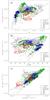 |
Fig. 11 Correlation plots of IFIR versus τ160, Td, and I8 μm, respectively. |
FIR intensity increases with increasing τ160, as Fig. 11a shows, but temperature differences play a role. The dust is comparatively hotter in PDR1 and PDR2, and in the CO-dark cloud. The FIR intensity scatters a lot when related to Td, as can be seen from Fig. 11b. Opposed to that, IFIR seems to be well-correlated to I8 μm (Fig. 11c).
4. Discussion
4.1. [C II] emission from the PDR
The total [C ii] luminosity from the mapped area of ≃ 210 sq. arcmin is Ltotal ≃ 14 L⊙. The luminosity stemming from the molecular cloud is Lcloud ≃ 13 L⊙ and that from the H ii region is LH ii ≃ 1 L⊙. Thus, about 5% of the total [C ii] luminosity of the surveyed area originates from the H ii region; 95% stems from the irradiated molecular cloud. This compares to 20% and 80%, respectively, of the area. For comparison, the total FIR luminosity from the mapped area is LFIR ≃ 1245 L⊙, of which 1210 L⊙ belong to the molecular cloud and 35 L⊙ to the H ii region. However, a small part of the luminosity may be attributed to NGC 2023: 0.2 L⊙ in [C ii] and 35 L⊙ in FIR luminosity. Since the 8 μm intensity as a cloud surface tracer is very well correlated to the [C ii] intensity, we may conclude that in the studied region of the Orion molecular cloud complex most of the [C ii] emission originates from PDR surfaces. This is in agreement with the distribution of [C ii] emission in OMC1: here, Goicoechea et al. (2015) find that 85% of the [C ii] emission arises from the irradiated surface of the molecular cloud. On Galactic scales, however, Pineda et al. (2014) find that ionized gas contributes about 20% and dense PDRs about 30% to the total [C ii] luminosity (the remainder stemming in equal amounts from cold H i gas and CO-dark H2 gas).
The [C ii] line-integrated intensity I[ C ii ] ranges from 10-5 erg s-1 cm-2 sr-1 in the H ii region up to a maximum of 7 × 10⁻⁴ erg s-1 cm-2 sr-1 in PDR1, with an average over the mapped area of  . The [C ii] cooling efficiency η = I[ C ii ]/IFIR takes its highest values at the edge of the molecular cloud, bordering on the Hα emitting region. Its peak value is about 3 × 10⁻², ranging down to 3 × 10⁻³. The separation of molecular cloud and H ii region emission is not trivial, since we think that the surface of the cloud is not straight, but warped. However, [C ii] emission from the region exclusively associated with the ionized gas in IC 434 is very weak and has a much wider line profile (cf. Figs. 6 and 12; see also Sect. 4.2). Hence, we assume that at the edge of the molecular cloud the [C ii] and FIR emission from ionized gas is minor compared to emission stemming from the molecular cloud itself.
Considering the average [C ii] cooling efficiencies, where beam-dilution and column-length effects should divide out, we note that PDR2 has twice as high [C ii] cooling efficiency as the Horsehead PDR and PDR1 have (see Table 1). We remark that PDR2 lies in a region where there still is significant Hα emission, indicating a corrugated edge structure. Since the average [C ii] emission in the H ii region is quite low, we do not expect [C ii] emission from the ionized gas to be responsible for the enhanced [C ii] cooling efficiency in PDR2. However, IFIR is unexpectedly low in PDR2, which may account for the mismatch in I[ C ii ]/IFIR.
4.2. [C II] emission from the H II region
From the Hα emission in the studied region, originating from the ionized gas to the west of the molecular cloud, we can estimate the density of the H ii region (Ochsendorf et al. 2014). The radiated intensity of the Hα line can be calculated by  (4)Assuming a gas temperature of T ≃ 104 K, we use 4πjHβ/npne = 8.30 × 1026 erg cm3s-1 and jHα/jHβ = 2.86 (Osterbrock 1989). Further, we assume a homogeneous gas distribution along the line of sight, which we take to be d ~ 1 pc. Hence, we obtain
  (5)where np = ne. When a molecular cloud is photoevaporated into a cavity, as the surface of L1630 is, we expect an exponential density profile as a function of distance from the surface. Fitting an exponential to the observed Hα emission along a line cut, we obtain a density law with ne,0 = 95 cm-2 at the ionization front and a scale length of 1.2 pc, which is in good agreement with Ochsendorf et al. (2014). In the surveyed area, the density varies between 60 and 100 cm-3.
Applying again T ≃ 104 K for the gas temperature to the cooling law of [C ii] (Eq. (2.36) in Tielens 2010), we obtain 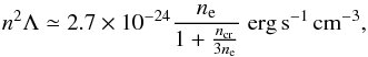 (6)where we assumed an ionization fraction of x = 1 and, hence, consider collisions with electrons only; the critical density scales with T and is, at T = 104 K, ncr ≃ 50 cm-3 (Goldsmith et al. 2012). Neglecting
  and assuming again d ~ 1 pc for the length of the line of sight, the above yields
 ![Mathematical equation: \begin{eqnarray} I_{\mathrm{[C\,\textsc{ii}]}} \simeq 7\times 10^{-5} \left(\frac{n_{\rm e}}{10^2\,\mathrm{cm}^{-2}}\right)\;\mathrm{erg\,s^{-1}\,cm^{-2}\,sr^{-1}}. \end{eqnarray}](/articles/aa/full_html/2017/10/aa30881-17/aa30881-17-eq263.png) (7)The observed intensity values lie in the range of 10-5 − 10-4 erg s-1 cm-2 sr-1, which is, given the range of densities, in good agreement with the values derived from Hα emission. However, it is difficult to recognize a declining trend in the [C ii] intensity away from the molecular cloud, since the signal is very noisy in the H ii region due to the low intensity.
(7)The observed intensity values lie in the range of 10-5 − 10-4 erg s-1 cm-2 sr-1, which is, given the range of densities, in good agreement with the values derived from Hα emission. However, it is difficult to recognize a declining trend in the [C ii] intensity away from the molecular cloud, since the signal is very noisy in the H ii region due to the low intensity.
 |
Fig. 12 [C ii] spectra towards the H ii region, averaged over 156 (left) and 187 (right) pixels. The left panel represents the H ii region north of the Horsehead Nebula, the right panel represents the part south of the Horsehead Nebula. For the northern part, we obtain TP = 1.0 K, FWHM = 8.7 km s-1, and vP = 14.1 km s-1; for the southern part, a Gaussian fit yields TP = 0.7 K, FWHM = 5.2 km s-1, and vP = 11.2 km s-1. |
The [C ii] spectra extracted from the H ii region show a very weak and very broad feature (Fig. 12) with a peak main-beam temperature of ~ 1 K and an FWHM of 5 − 10 km s-1, as compared to 10 − 20 K and 2 − 4 km s-1 for the PDR regions in the molecular cloud. This is distinct from the spectra taken towards the cloud. We cannot distinguish a broad feature in the spectra taken towards the molecular cloud, although there is some Hα emission and we should expect ionized gas in front of the multiple PDR surfaces. Most likely the intensity is simply too low, approximately ten times lower than the intensity towards the H ii region, assuming that the H ii column in front of the molecular cloud as seen along the line of sight is ~ 0.1 pc, which renders the signal undetectable.
4.3. FIR emission and beam-dilution effects
We expect that beam dilution affects all maps to some extent when convolved to the SPIRE 500 μm36″ resolution, since the unconvolved IRAC 8 μm map at 1.98″ resolution reveals features and delicate structures (see Fig. 15) that disappear upon convolution. The upGREAT beam has an FWHM of 15.9″, thus beam dilution might be noticeable in [C ii] observations towards thin filaments. From the IRAC 8 μm emission, we infer a dilution factor of ~ 2.5 for the Horsehead PDR going from the native resolution of the 8 μm image to 36″ resolution, but only for the narrowest (densest) part of the PDR. The average 8 μm emission is not significantly beam-diluted when convolved to 36″. PDR3 possibly suffers significantly from beam dilution as well, since it shows as a rather sharp filament in 8 μm, where it reaches high peak values (higher than the Horsehead PDR peak values). Values of quantities we observe and compute from that are taken to be beam-averaged values in the respective resolution.
Due to the edge-on geometry of the PDRs in L1630 with respect to the illuminating star system σ Ori (and the low dust optical depth), we expect that IFIR depends on the re-radiating column along the line of sight, which might explain the excess intensity in 8 μm, [C ii], and FIR in PDR1 as compared to other PDR surfaces here. The commonly expected value of incident FUV radiation, re-emitted in IFIR, is G0 ≃ 100, calculated from properties of σ Ori (Abergel et al. 2003, and references therein). Given the edge-on geometry of the cloud-star complex, the formula by Hollenbach & Tielens (1999), 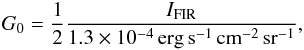 (8)cannot be used to infer the intensity of the incident UV radiation. The FIR intensity varies substantially across the mapped area; for a face-on geometry with a single UV-illuminating source, one would expect less divergent values. This realization corroborates the assumption of an edge-on geometry and has been the rationale for building edge-on models with different molecular-cloud depths along the line of sight.
The dust optical depth τ160 does not trace the PDR surface column, but the total gas and dust column. The FIR intensity does not increase with increasing τ160 for PDR1, PDR2, and PDR3 (in comparison to τ160 ≃ 2 × 10⁻³, 1 × 10⁻³, 3 × 10⁻³, respectively5). Especially in the case of PDR3, τ160 likely traces not only the PDR but the molecular cloud interior, as well. A fraction of IFIR might stem from deeper, cooler parts of the molecular cloud and not from the PDR surface, although IFIR is biased towards the hot PDR surface, as is τ160. In PDR2, IFIR is lower than we would expect, leading to significantly higher I[ C ii ]/IFIR than in PDR1 and PDR3. The dust temperature Td in PDR2 is determined to be considerably lower than in PDR1, although the environments seem similar.
4.4. Column densities, gas temperature, and mass
Since we do not detect the [13C ii] line in single spectra, we cannot determine the [C ii] optical depth by means of it. The noise rms of the spectra is too high to put a significant constraint on τ[ C ii ]. In averaged spectra, we can detect the [13C ii] F = 2 − 1 line just above the noise level (see Sect. 4.5). However, knowing the C+ column density and the intrinsic line width, we can estimate the [C ii] optical depth and the excitation temperature (see Appendix A) from single spectra. We compute the C+ column density of the PDR surface from the dust optical depth, assuming standard dust properties and that all carbon in the PDR surface is singly ionized. Additionally, we expect beam dilution to be insignificant for the [C ii] observations. From the native IRAC 8 μm map, we infer a dilution factor of 1.5 when going to 15.9″ resolution, but only towards the thinnest filament in the Horsehead mane. This equally yields a peak temperature of TP ≃ 20 K there, as does the brightest part of the Horsehead PDR.
The gas column density can be computed from the dust optical depth τ160, assuming a theoretical absorption coefficient. This yields 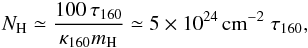 (9)where we have used a gas-to-dust mass ratio of 100 and assumed κabs = 2.92 × 10⁵(λ [ μm ] )-2 cm2 / g (Li & Draine 2001). With the fractional gas-phase carbon abundance [ C / H ] = 1.6 × 10⁻⁴ (Sofia et al. 2004), we can estimate the C+ column density in the PDR surface from the dust optical depth, under the assumption that all carbon in the line of sight is ionized:
  (10)Later studies have reported somewhat differing values for [ C / H ], varying by a factor of two for different sight lines (see e.g. Sofia & Parvathi 2009; Sofia et al. 2011). However, the average is not found to deviate substantially from the earlier value of [ C / H ] = 1.6 × 10⁻⁴; the general uncertainty seems to be quite large. We discuss the effect of the uncertainty in the column density on the derived gas properties in the following. For PDR1 and PDR2 we have τ160 ≃ 2 × 10⁻³ and τ160 ≃ 10-3, respectively, from the τ160 map, where we assume that all the dust actually is in the PDR surface. However, these values for the dust optical depth may be affected by significant uncertainties, up to a factor of two, since τ160 depends on the assumed dust properties in the SED fit (see discussion in Sect. 2.2). For PDR3, we suppose that there is a significant amount of cold material located along the line of sight, which renders τ160 an inaccurate measure for the depth of the PDR along the line of sight here.
Inferring the PDR dust optical depth of the Horsehead PDR requires further effort. According to Habart et al. (2005), there is a large density gradient from the surface to the bulk of the Horsehead PDR. In the surface the gas density might be as low as nH ~ 104 cm-3, whereas in the bulk it assumes nH ~ 2 × 105 cm-3. Abergel et al. (2003) find nH ~ 2 × 104 cm-3 as a lower limit for the density of the gas directly behind the illuminated filament. The dust optical depth is likely to be beam diluted in the SPIRE 500 μm resolution; the filament has an extent of only 5 − 10″. Assuming that the maximum τ160 ≃ 10-2 occurs in the densest (inner) part of the PDR and that the length along the line of sight remains approximately the same, we conclude that the dust optical depth in the Horsehead PDR surface must be significantly lower than the maximum value, by a factor of approximately ten, due to the decreased density.
From deep integration of the Horsehead PDR with SOFIA/upGREAT, however, we are able to infer a [C ii] optical depth of τ[ C ii ] ≃ 2 from the brightest [13C ii] line, which can be detected in these data (C. Guevara, priv. comm.; Guevara et al., in prep.). According to Eq. (A.5), this translates into a C+ column density of NC+ ≃ 7 × 1017 cm-2, that is τ160 ≃ 10-3, which is ten times lower than the maximum value in the Horsehead bulk. However, from our models, this [C ii] optical depth corresponds to a twice as large C+ column density of NC+ ≃ 1.6 × 1018 cm-2, if we assume that all carbon is ionized within our beam, which might not be the case.
We calculate the [C ii] optical depth τ[ C ii ] and excitation temperature Tex for PDR1 and PDR2, and Tex for the Horsehead PDR, using the formulas of Appendix A6. The results are shown in Table 3. In principle, the values we infer for NC+ are upper limits, but the general uncertainty in the C+ column density is potentially larger than the deviation from the upper limit. The dust optical depth, from which we calculate the C+ column density, is not well-determined (cf. Sect. 2.2) and the carbon fractional abundance may deviate. If we assume an error margin of the C+ column density of ±50%, this results in ranges of [C ii] optical depth and excitation temperature of τ[ C ii ] ≃ 0.6 − 2.7 and Tex ≃ 60 − 90 K, respectively, for PDR1, and τ[ C ii ] ≃ 0.4 − 2.2 and Tex ≃ 60 − 100 K, respectively, for PDR2. Certainly, these values are subject to uncertainties in the inferred gas density and the spectral parameters, as well; however, the uncertainty in NC+ seems to be the most significant, leading to considerable deviations, so we will not discuss the influence of the other uncertainties here. In the Horsehead PDR, the precise value of τ[ C ii ] does not overly influence the excitation temperature which we calculate: it is Tex ≃ 60 ± 2 K.
If the density of the gas is known, one can compute the gas temperature from the excitation temperature:  (11)with the critical density
 ![Mathematical equation: \hbox{$n_{\mathrm{cr}}=\beta(\tau_{\mathrm{[C\,\textsc{ii}]}})\frac{A}{\gamma_{\mathrm{ul}}}$}](/articles/aa/full_html/2017/10/aa30881-17/aa30881-17-eq313.png) , where β(τ[ C ii ]) is the [C ii] 158 μm photon escape probabilty, A ≃ 2.3 × 10⁻⁶ s-1 is the Einstein coefficient for spontaneous radiative de-excitation of C+, and γul is the collisional de-excitation rate coefficient, which is γul ≃ 7.6 × 10⁻¹⁰ cm3 s-1 for C+–H collisions (Goldsmith et al. 2012) and γul ≃ 5.1 × 10⁻¹⁰ cm3 s-1 for C+–H2 collisions (Wiesenfeld & Goldsmith 2014) at gas temperatures of ≃ 100 K; n is the collision partner density. At T ~ 100 K,γul, and thereby ncr, is only weakly dependent on temperature; for C+–H collisions, ncr ≃ β(τ[ C ii ]) × 3.0 × 103 cm-3, and for C+–H2 collisions, ncr ≃ β(τ[ C ii ]) × 4.5 × 103 cm-3. At the cloud edge, collisions with H dominate the excitation of C+, while deeper into the cloud H2 excitation dominates. We expect that excitation caused by collisions involving both H and H2 contribute within our beam. Since the points we chose in PDR1 and PDR2 lie close to the surface, we consider collisions with H; in the Horsehead PDR the choice of collision partner does not affect the derived gas temperature significantly due to the higher gas density. We take the photon escape probability to be β(τ) = (1 − e− τ) /τ, as used in our edge-on PDR models. The densities are discussed in Sect. 4.7.
, where β(τ[ C ii ]) is the [C ii] 158 μm photon escape probabilty, A ≃ 2.3 × 10⁻⁶ s-1 is the Einstein coefficient for spontaneous radiative de-excitation of C+, and γul is the collisional de-excitation rate coefficient, which is γul ≃ 7.6 × 10⁻¹⁰ cm3 s-1 for C+–H collisions (Goldsmith et al. 2012) and γul ≃ 5.1 × 10⁻¹⁰ cm3 s-1 for C+–H2 collisions (Wiesenfeld & Goldsmith 2014) at gas temperatures of ≃ 100 K; n is the collision partner density. At T ~ 100 K,γul, and thereby ncr, is only weakly dependent on temperature; for C+–H collisions, ncr ≃ β(τ[ C ii ]) × 3.0 × 103 cm-3, and for C+–H2 collisions, ncr ≃ β(τ[ C ii ]) × 4.5 × 103 cm-3. At the cloud edge, collisions with H dominate the excitation of C+, while deeper into the cloud H2 excitation dominates. We expect that excitation caused by collisions involving both H and H2 contribute within our beam. Since the points we chose in PDR1 and PDR2 lie close to the surface, we consider collisions with H; in the Horsehead PDR the choice of collision partner does not affect the derived gas temperature significantly due to the higher gas density. We take the photon escape probability to be β(τ) = (1 − e− τ) /τ, as used in our edge-on PDR models. The densities are discussed in Sect. 4.7.
Using nH ≃ 3 × 103 cm-3 for PDR1 and PDR2, we obtain T ≃ 86 K and T ≃ 93 K, respectively, for C+–H collisions. In the Horsehead PDR, we compute T ≃ 60 K. From models (see Sects. 3.4 and 4.9) we compute a gas temperature of about T ≃ 100 − 140 K in the top layers of a PDR (cf. Fig. 7). This is in reasonable agreement with the values derived from our observations in PDR1 and PDR2. In the Horsehead PDR, however, the results likely are affected by beam dilution, since the gas temperature drops quickly on the physical scale (within the beam size of 15.9″ of the [C ii] observations). Disregarding this, with a low C+ column density of NC+ = 1.6 × 1017 cm-2 we can match the gas temperature measured by Habart et al. (2011) from H2 observations, T ≃ 264 K; this results in a [C ii] optical depth of τ[ C ii ] ≃ 0.1. We can fit a gas temperature of T ≃ 120 K, as predicted by our models for conditions appropriate for the Horsehead PDR, with a column density of NC+ ≃ 2.0 × 1017 cm-2. This would yield a [C ii] optical depth of τ[ C ii ] ≃ 0.3. Both values are significantly lower than what is observed in [13C ii].
According to Goldsmith et al. (2012), the [C ii] line is effectively optically thin, meaning the peak temperature is linearly proportional to the C+ column density, if TP<J(T) / 3, where J(T) is the brightness temperature of the gas. Hence, even though our derived [C ii] optical depth for PDR1 and PDR2 is >1, the line is still effectively optically thin in these regions. It is optically thick in the Horsehead PDR.
From the H column densities, that is, from the dust optical depth, we can estimate the mass of the gas: Mgas = NHmHA, where A is the surface that is integrated over. The total gas mass of the molecular cloud (not including the H ii region IC 434 and the north-eastern corner of gas and dust associated with NGC 2023) in the [C ii] mapped area is Mgas,total ≃ 280 M⊙. The Horsehead Nebula and its shadow add Mgas ≃ 33 M⊙ to the total mass, the Horsehead PDR surface contributing Mgas ≃ 3 M⊙. The mass of CO-emitting gas (also computed from NH) is Mgas ≃ 250 M⊙. The assumption that CO-emitting gas contributes the bulk of the mass and that [C ii] traces PDR surfaces yields a gas mass of PDR surfaces of Mgas ≃ 20 M⊙. Additionally, ≃ 12 M⊙ are located in gas that emits neither strongly in [C ii] nor in CO. The H ii region comprises Mgas ≃ 10 M⊙ as derived from the dust optical depth; from Hα emission, we estimate Mgas ≃ 5 M⊙.
Table 4 compares the masses computed from the dust optical depth and from CO (1 − 0) emission, respectively, for the several regions we defined. Since the uncertainties (in the dust optical depth, but also in the conversion factors, especially in the XCO factor Bolatto et al. cf. 2013) are substantial, we cannot draw clear-cut conclusions. We note, moreover, that PDR regions might overlap along the line of sight with CO-emitting regions whose emission stems from a different layer of the molecular cloud, as certainly is the case in PDR3. It seems that there is a fair amount of gas mass unaccounted for by CO emission, but within the error margin of 30%, this mass can be between 10 and 100 M⊙. In a larger area mapped in CO, comprising the area mapped in [C ii], Pety et al. (2017) find that the CO-traced mass is in fact greater than the dust-traced mass; this especially influences the deeper layers of the Orion B molecular cloud (see Table 4 in Pety et al. 2017), thus these findings might not apply to our study field in L1630. However, they conclude that CO tends to overestimate the gas mass, whereas the dust optical depth underestimates it. In this way, with an area of ~2 pc2, we find a gas mass surface density of 100 − 150 M⊙ pc-2 in the [C ii] mapped area.
4.5. Excitation properties from [13C II]
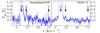 |
Fig. 13 [C ii] spectra towards the Horsehead PDR and PDR1+2, averaged over 180 (left) and 3140 (right) pixels. Arrows indicate the positions of the [12C ii] line and the [13C ii] F = 2 − 1 and F = 1 − 1 lines (from left to right); the [13C ii] F = 1 − 0 line falls outside the spectral range of our map. |
If we average over a large number of spectra in [C ii]-bright areas, we are able to identify the [13C ii] F = 2 − 1 line above the 5σ level (see Fig. 13); we cannot detect the other two (weaker) [13C ii] lines. From the [13C ii] F = 2 − 1 line, we can compute average values of the [C ii] optical depth, the excitation temperature, and the C+ column density. From an average spectrum of the [C ii]-bright regions of PDR1 and PDR2 (an area of 50 square arcmin, which is a third of the cloud area and corresponds to 3140 spectra), we obtain τ[ C ii ] ≃ 1.5 (with an uncertainty of 20%). To obtain this result, we used [13C ii] line parameters established by Ossenkopf et al. (2013) and the 12C/13C isotopic ratio of 67 for Orion (Langer & Penzias 1990; Milam et al. 2005). This yields a C+ column density of NC+ ≃ 3 × 1017 cm-2. From an average over the Horsehead PDR (an area of 3 square arcmin, corresponding to 180 spectra), we obtain τ[ C ii ] ≃ 5 (also with 20% uncertainty) and NC+ ≃ 1 × 1018 cm-2. We note that τ[ C ii ] in PDR1 and PDR2 does match the value calculated in Sect. 4.4 from the dust optical depth and single spectra, and NC+ does not, whereas in the Horsehead PDR τ[ C ii ] does not agree, but NC+ does. Excitation temperatures from the averaged spectra are Tex ≃ 40 K, which is lower than what we infer from single spectra. Regions with lower-excitation [C ii] contribute to the averaged spectra, but we have to include them to obtain a sufficient signal-to-noise ratio. We stress that this spectral averaging over a large area with varying conditions will weigh the emission differently for the [12C ii] and [13C ii] lines in accordance with the excitation temperatures and optical depths involved. Hence, the averaged spectrum will not be the same as the spectrum of the average. In our analysis, we have elected to rely on the analysis based on the dust column density rather than this somewhat ill-defined average.
4.6. Photoelectric heating and energy balance
The most substantial heating source of PDRs is photoelectric heating by PAHs, clusters of PAHs, and very small grains. The photoelectric heating rate is deeply built into PDR models and controls the detailed structure and emission characteristics to a large extent. The heating rate drops with increasing ionization of these species. It can be parametrized by the ionization parameter γ = G0T0.5/ne, where G0 is the incident radiation, T is the gas temperature, and ne is the electron density; the corresponding theoretical curve as derived by Bakes & Tielens (1994) is shown in Fig. 14. Okada et al. (2013) confirm in a study of six PDRs, which represent a variety of environments, the dependence of the photoelectric heating rate on PAH ionization and conclude on the dominance of photoelectric heating by PAHs.
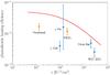 |
Fig. 14 Theoretical photoelectric heating efficiency of PAHs, clusters of PAHs, and very small grains is plotted against the ionization parameter γ = G0T0.5/ne (Bakes & Tielens 1994). We added the orange data points for the Horsehead PDR and PDR1. Blue data points are for the diffuse-ISM sight lines ζ Oph and o Per, and the PDRs Orion Bar and NGC 2023. Figure adapted from Tielens (2008). |
The [C ii] 158 μm cooling rate increases with gas density and temperature. In the high-density limit (nH ≫ ncr), it scales with nH, whereas for low densities it scales with  ; the temperature dependence is largely captured in a factor exp( − ΔE/kBT), where ΔE is the energy level spacing.7 The gas density of the Horsehead PDR, nH ≃ 4 × 104 cm-3, lies above the critical density for C+, ncr = β(τ[ C ii ]) × 3.0 × 103 cm-3; the densities of PDR1 and PDR2 are close to ncr, that is, in the intermediate density regime. The similar gas temperatures and densities of PDR1 and PDR2, however, do not reflect the difference in the [C ii] cooling efficiencies I[ C ii ]/IFIR calculated in Table 1 and visualized in Fig. 8a (cf. Sect. 4.3). In the case of the Horsehead PDR, gas cooling through the [O i] 63 μm line becomes important; the [O i] surface brightness is comparable to the surface brightness of the [C ii] line (Goicoechea et al. 2009).
We emphasize that we can directly measure the temperature and the density of the emitting gas in the PDR from our observations (see Sects. 4.4 and 4.7, respectively). Hence, we can test the theory in a rather direct way. Specifically, we assume that all electrons come from C ionization, hence ne = 1.6 × 10⁻⁴nH, where we have adopted the gas-phase abundance of carbon estimated by Sofia et al. (2004). For the Horsehead PDR with nH ≃ 4 × 104 cm-3 and T ≃ 60 K, we compute an ionization parameter of γ ≃ 1 × 10² K1 / 2 cm3; for PDR1 and PDR2 with nH ≃ 3 × 103 cm-3 and T ≃ 100 K, we obtain γ ≃ 2 × 10³ K1 / 2 cm3. From the cooling lines, that is, assuming that all the heating is converted into [C ii] and [O i] emission, we arrive at a heating efficiency of 1.7 ± 0.4 × 10⁻² (with I[ O i ] ≃ 1.04 ± 0.14 erg s-1 cm-2 sr-1 from Goicoechea et al. 2009, at similar spatial resolution) for the Horsehead PDR, and 1.1 ± 0.3 × 10⁻² for PDR1. From their [O i] study of the Horsehead Nebula, Goicoechea et al. (2009) find a heating efficiency of 1 − 2 × 10⁻², which is consistent with our findings. For PDR2, we calculate an average [C ii] cooling efficiency of 2.2 ± 0.4 × 10⁻². However, IFIR is unexpectedly low in PDR2, so we wonder whether the mismatch in I[ C ii ]/IFIR between PDR1 and PDR2 really is due to an erroneous determination of IFIR and is thereby deceptive.
The general behavior of the observationally obtained heating efficiency is indeed very similar to the theoretical curve for photoelectric heating by PAHs, clusters of PAHs, and very small grains, as shown in Fig. 14, except that theoretical values seems to be offset to higher efficiency by about a factor of two. Such a shift might reflect a somewhat different abundance of PAHs and related species in the studied regions. We note that these differences between theory and observations can lead to considerable differences in the derived physical conditions. For example, adopting the theoretical relationship and solving the energy balance for the gas density and FUV field appropriate for the Horsehead PDR would result in a derived gas temperature of T ≃ 100 K, while the temperature as measured from the pure rotational H2 lines by Habart et al. (2011) is T ≃ 264 K, and we determine it to be T ≃ 60 K, which is beam-averaged. For PDR1 and PDR2, the theoretical relationship would imply a temperature of T ≃ 125 K, while we measure T ≃ 90 K from the peak [C ii] intensity. From a theoretical perspective, we expect the temperature to decrease with increasing density (cf. Fig. 9.4 in Tielens 2010). This is what we see in [C ii] observations. However, from studies by Habart et al. (2011) and Habart et al. (2005), the observational temperature lies in the regime T ≃ 200 − 300 K, albeit in a very narrow surface gas layer. Here, the observational temperature in the Horsehead PDR appears to be higher than the theoretical temperature, despite the heating efficiency being underestimated. This may seem inconsistent; it certainly suggests that we have to be very careful with the assumptions we make. However, the discrepancy may be due to various reasons, not all of them implying inconsistency, that we will not discuss in this paper. Calculating the ionization parameter with either differing observational temperatures or the theoretical temperature does not shift the data points in Fig. 14 significantly towards the theoretical curve. Clearly, further validation of the theoretical relationship in a variety of environments is important as photoelectric heating is at the core of all PDR research, including studies on the phase structure of the ISM (Wolfire et al. 1995, 2003; Hollenbach & Tielens 1999). The significance of PAH photoelectric heating is reflected in the tight correlation between PAH and [C ii] emission from the PDRs (see Figs. 8f and 19d). In a future study, we intend to return to this issue of the importance of PAHs to the heating of interstellar gas.
4.7. Line cuts
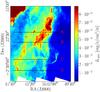 |
Fig. 15 IRAC 8 μm image with lines A, B, C, and D indicated. |
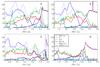 |
Fig. 16 IRAC 8 μm (PAH) intensity, Hα intensity, [C ii] and CO (1 − 0) line-integrated intensity, PACS 160 μm intensity, and SCUBA 850 μm intensity plotted in their respective native resolution along lines A, B, C, and D of Fig. 15 in their respective original spatial resolution. Multiply plotted values by 1.4 × 10⁻⁴, 2.9 × 10⁻³, 7.0 × 10⁻⁶, 1.6 × 10⁻⁹, 3,9 × 10⁻⁵, and 2.2 × 10⁻⁷, respectively, for I8 μm, IHα, I[ C ii ], ICO (1 − 0), I160 μm, and I850 μm, respectively, in erg s-1 cm-2 sr-1. |
The edge-on nature of the PDR in the Orion B molecular cloud (L1630) is well illustrated by line cuts taken from the surface of the molecular cloud into the bulk (cf. Figs. 15 and 16). In addition to previously employed tracers (8 μm, Hα, [C ii], CO (1 − 0)), we compare with SCUBA 850 μm observations, that trace dense clumps, and compare PACS 160 μm data as a measure for IFIR.
Along line cut C, the Horsehead PDR is clearly distinguishable; Hα drops immediately and the other four tracers peak, which indicates high density. Assuming AV = 2 for the transition from C+/C to CO and NH = 2 × 1021 cm-2AV, which is consistent with our models (see Fig. 7), we obtain from the physical position of the transition, d ≃ 0.03 pc, nH ≃ 4 × 104 cm-3. Since there are no further indications of dense clumps in 850 μm emission, we assume that the rest of the gas located along cut C is relatively diffuse. Having established that, we tentatively assign the CO peak between 0.6 and 0.8 pc to the PDR surface at 0.3 pc. We infer a gas density of nH ≃ 3 × 103 cm-3. Identifying the CO peak at 1.1 pc with the PDR surface at 0.6 pc yields about the same density.
If we perform the same procedure for line cut A, we derive about the same densities, nH ≃ 3 × 103 cm-3. Here, we assign the broad prominent CO feature at 0.8 pc to the broad PDR feature at 0.4 pc. The small CO peak at 0.5 pc possibly relates to the PDR feature at 0.4 pc, hence nH ≃ 104 cm-3. The broad CO feature between 0.2 and 0.4 pc could originate from a dense surface, located at 0.2 pc.
Line cut B is difficult to interpret. Due to their respective shapes, the PAH peaks around 0.6 pc might correspond to the CO peaks at 0.7 and 0.85 pc, yielding a density of nH ≃ 5 × 10³ − 104 cm-3. There is no indication of dense clumps in the SCUBA map at this point. The gas at the surface is likely to be relatively diffuse, since there is no distinct CO peak that could be related.
The gas at the surface cut by line D is denser again. Here, we estimate nH ≃ 3 × 104 cm-3. PDR3 at 1.0 pc might be relatively dense too, since there is CO emission peaking directly behind the PDR front. However, this CO emission could certainly originate from deeper, less dense layers of the molecular cloud, as well. There is no 850 μm peak corresponding to the CO peak, rendering the latter hypothesis more plausible.
There are a number of CO peaks we cannot relate to a specific structure, for example, the one at 0.4 pc in line cut C. This might indicate that there are layers of gas with higher density stacked along the line of sight. Overall, this analysis suffers from numerous uncertainties and unknowns. Nevertheless, the calculated densities seem to be reasonable for a molecular cloud.
4.8. Geometry of the L1630 molecular cloud
 |
Fig. 17 Geometry of the L1630 molecular cloud surface. |
Our data suggest that the L1630 molecular cloud as we see it consists of stacked layers of PDRs along the line of sight, which are offset against each other. Figure 17 shows a schematic illustration, which we inferred from our data, of the edge-on geometry of the studied region of the Orion B molecular cloud. The surface of the molecular cloud is inclined with respect to the incident radiation and the observer, but with steps where strong PDR surfaces can be discerned in the IRAC 8 μm image, for instance. This implies that we generally cannot compare our data with face-on PDRs; in the correlation plots, we need to correlate along line cuts and not along the line of sight. Also, the incident radiation is not easily estimated (see discussion in Sect. 4.3).
The CO emission in the Horsehead neck stems from a different distance along the line of sight than the overlapping [C ii] emission. The CO emission stems from the shadow of the Horsehead Nebula, whereas IFIR and I[ C ii ] originate from the surface of the bulk molecular cloud. They are spatially not coincident and are likely to correspond to different densities. Hence, the [C ii] and the CO emission from this part cannot be correlated.
We do not see sharp Hα edges along the line cuts, as we would expect for multiple PDR fronts, but only on the primary surface of the molecular cloud. We clearly notice the onset of the bulk cloud behind the Horsehead Nebula in line cut C, and in line cut D there is a distinct shoulder to the primary Hα peak. Apart from that, the Hα emission across the molecular cloud is somewhat diffuse. We do notice coincidence, however, between the Hα emission contours and the PDR surfaces as traced by [C ii] emission. In Fig. 18, PDR1 and PDR2 are lined-out by contours of high IHα, whereas PDR3 and the intermediate PDR fronts are traced by contours of lower IHα.
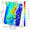 |
Fig. 18 Original [C ii] image (line-integrated intensity) with Hα emission in contours (slightly smoothed). Contours from black to white: IHα = 0.5,1.0,2.0,3.0,4.0,5.0,6.0 × 10-3 erg s-1 cm-2 sr-1. |
 |
Fig. 19 Correlation plots for L1630 (Orion B) and OMC1 (Orion A); the OMC1 data are convolved to 25″ resolution, L1630 data to 36″ resolution. CO data are for the CO (1 − 0) line in L1630 and for the CO (2 − 1) line, divided by 8 (see Sect. 4.10), in OMC1. |
From the dust optical depth and the inferred densities, we can estimate the length of the PDR along the line of sight. At the surface of the Horsehead Nebula, τ160 ≃ 10-3 together with nH ≃ 4 × 104 cm-3 yields an estimate of about lPDR ≃ 0.05 pc. In the bulk, however, we would expect something closer to the projected extent, about ≃ 0.2 pc. Assuming a density of nH ≃ 2 × 104 cm-3, Habart et al. (2005) arrive at lPDR ≃ 0.5 pc, but comment that this seems implausibly high; they conclude that the density must actually be higher. If we adopt nH ~ 2 × 105 cm-3 (Habart et al. 2005) for the bulk and a dust optical depth of τ160 ≃ 10-2, we obtain lHorsehead ≃ 0.17 pc.
For PDR1 and PDR2, we estimate lPDR1 ≃ 1 pc and lPDR2 ≃ 0.5 pc, respectively. PDR3 yields lPDR3 ≃ 1.5 pc, but this is most likely not the length of the PDR but of the whole PDR+molecular cloud interior column. From the G0 values of Sect. 4.3, assuming that G0 ∝ lPDR, we infer that lPDR3 lies in between lPDR1 and lPDR2.
4.9. Comparison with models
As described in Sect. 3.4, we ran PDR models for an edge-on geometry with varying length along the line of sight and varying density (see also Fig. 7) at G0 = 100. The respective model relations between tracers are plotted in Figs. 8a, b, e, and 9: I[ C ii ]/IFIR versus IFIR, I[ C ii ] versus IFIR, I[ C ii ] versus ICO (1 − 0), and I[ C ii ]/IFIR versus ICO (1 − 0)/IFIR, respectively.
We have constructed models for selected depths of the molecular cloud along the line of sight AV,los, which we calculated from the gas column density using NH = 2.0 × 1021 cm-2AV, and gas densities nH, that we inferred from τ160 in Sect. 4.4 and the line cuts in Sect. 4.7, respectively. For PDR1, we estimated AV,los ≃ 5.0, whereas for PDR2 we got AV,los ≃ 2.5. The Horsehead PDR ranges from AV,los ≃ 2.5 at the edge to AV,los ≳ 5.0 deeper in the Horsehead Nebula. For the gas in PDR1 and PDR2, we assume nH = 3.0 × 103 cm-3; for the Horsehead PDR we take nH = 4.0 × 104 cm-3, but we note that the density increases with depth into the PDR according to a number of studies on that region (cf., e.g., Habart et al. 2005). Further, we ran models for nH = 1.6 × 104 cm-3 to probe a density region that might either be occupied by the Horsehead PDR or by a denser (surface) structure overlaid on PDR1 and PDR2.
Figure 8a shows that the model predictions for the Horsehead with AV,los = 0.5 and nH = 1.6 × 104 cm-3 or nH = 4.0 × 104 cm-3 are consistent with the data, whereas we estimated AV,los = 2.5. The AV,los = 2.5 line with nH = 4.0 × 104 cm-3 could fit the data within the extent of beam dilution. The AV,los = 5.0 model lines cannot explain the data, even when taking into account beam-dilution effects. Another reason for the discrepancy might be dust depletion in this region decreasing the FIR emission. PDR1 is matched quite well by the curve for AV,los = 5.0 and nH = 3.0 × 103 cm-3, but the data points lie close to the AV,los = 2.5 with nH = 3.0 × 103 cm-3 line, as well. The latter also fits PDR2 quite well. The rest of the data points lie between these two curves and the curves for AV,los = 0.5. Similar conclusions can be drawn for Fig. 8b. The PDR data points are matched by the same model curves as before, with the remaining points lying in between these and the AV,los = 0.5 curves.
The comparison of the data with the model predictions for the relation between [C ii] and CO (1 − 0) is less clear-cut. In Fig. 8e, PDR1 and PDR2 lie close to the AV,los = 5.0 line. However, also the higher density lines agree with the data points in PDR1. The Horsehead points lie close to the AV,los = 2.5 lines instead of the AV,los = 5.0or0.5 lines. This might reflect the fact that AV,los = 2.5 in deeper layers of the Horsehead PDR, whereas it might be lower in the [C ii] emitting surface layers.
In Fig. 9, model lines group according to their respective densities and there is comparatively little variation with AV,los. PDR1 lies on the model lines with nH = 1.6 × 104 cm-3. This behavior might imply that the density deeper in the cloud in this region is increased. PDR2 lies on the nH = 3.0 × 103 cm-3 lines. All the AV,los lines for nH = 1.6 × 104 cm-3 run through the Horsehead data points, though some data points lie closer to the model lines for higher or lower density.
The gas temperatures in the top layers of the PDRs are predicted by the models as T ≃ 130 K for PDR1 and PDR2, and T ≃ 115 K for the Horsehead PDR. The latter again is a deviation from the value we infer, T ≃ 60 K, and the temperature estimated by Habart et al. (2011), which is T ≃ 264 K; it lies close to the value assumed by Goicoechea et al. (2009) for modeling [O i] emission from the Horsehead PDR, T ≃ 100 K, and close to the value deduced from equating the photoelectric heating efficiency with the [C ii]+[O i] cooling efficiency, T ≃ 100 K (cf. Sect. 4.6). For PDR1 and PDR2, the gas temperatures computed in Sect. 4.4 assuming excitation by C+–H collisions, T ≃ 90 K, are in good enough agreement with the value predicted by the model, especially considering the uncertainties. The derived temperatures would be substantially higher if we considered collisions with H2 to dominate the excitation of C+ (T ≃ 160 − 200 K); the contribution of C+–H2 collisions may be reflected in the underestimation of the gas temperature. Other reasons for slight discrepancies may be the uncertainties in gas density, the error margins of the spectral parameters that we used in the analysis, the uncertainty in the C+ column, and, of course, uncertainties within the models.
In conclusion, we are quite capable of reproducing the observed data with model data within the given uncertainties. Our AV,los and the gas densities can only be estimates, as is the geometry of the molecular cloud that probably has a corrugated surface and density gradients running through it.
4.10. Comparison with OMC1 in the Orion A molecular cloud
One of the aims of the present study is to establish correlations of astrophysical tracers under moderate conditions (intermediate density and moderate UV-radiation field) and to compare those to correlations found under harsher conditions (higher density and strong UV-radiation field). An example of the latter conditions is OMC1 in the Orion A complex. Whereas L1630 has edge-on geometry, OMC1 can be approximated as a face-on PDR with respect to its UV-illuminating sources, the Trapezium cluster. In this section, we compare the correlations found in L1630 to those in OMC1. Data on OMC1 are from Goicoechea et al. (2015).
The OMC1 data seem to continue the trend found in our L1630 data very well in Figs. 19a, b, and d. Both in OMC1 and in L1630, the 8 μm emission correlates well with I[ C ii ]. From a linear fit, we find I[ C ii ] ≃ 4.9 × 10⁻²I8 μm + 9.0 × 10⁻⁵ erg s-1 cm-2 sr-1 (ρ = 0.79), which is similar to the result of Goicoechea et al. (2015): I[ C ii ] ≃ 2.6 × 10⁻²I8 μm + 1.6 × 10⁻³ erg s-1 cm-2 sr-1 (ρ = 0.91). However, the slope of Goicoechea et al. (2015) should be divided by 2.9, since they use a bandwidth of the IRAC 8 μm band of 1 μm, whereas it is really 2.9 μm. Thus, there is some discrepancy, which expresses itself as a flattening of the correlation curve at high 8 μm and [C ii] intensity, comparable to the IFIR − I[ C ii ] dependency (Fig. 19a).
In Fig. 19c, the I[ C ii ]/IFIR versus ICO/IFIR relation in L1630 and OMC1 is shown. CO-line intensities in L1630 are from the CO (1 − 0) transition, whereas in OMC1 line intensities are from the CO (2 − 1) transition; we divide the CO (2 − 1) intensity in OMC1 by 8, the frequency ratio of the two lines cubed, which for optically thick thermalized CO emission as in OMC1 (cf. Goicoechea et al. 2015) gives a good estimate of the CO (1 − 0) intensity. The data points form two patches with different slopes. Yet, the L1630 data in their entirety seem to show a continuation of the trend set by the OMC1 data. We note that L1630 is characterized by a much higher I[ C ii ]/IFIR which reflects the decrease of photoelectric heating efficiency with increasing G0 and the importance of [O i] cooling for high G0 and high density. The difference in behavior of the I[ C ii ]/IFIR versus ICO/IFIR relation reflects the difference in geometry. As demonstrated in the study of Goicoechea et al. (2015), OMC1 is well-modeled as a face-on PDR, while L1630 has edge-on geometry (cf. Fig. 9).
Goicoechea et al. (2015) find a decrease of I[ C ii ]/IFIR with dust temperature, which is notably different from our observation shown in Fig. 8d; we find no significant slope. Also, we obtain a less good correlation of IFIR with τ160 than do Goicoechea et al. (2015) for OMC1 (cf. Sect. 3.5, Fig. 11a). The figure corresponding to Fig. 10 in our paper, I[ C ii ]/IFIR versus τ160, in Goicoechea et al. (2015), reveals that OMC1 matches a slab of constant foreground [C ii] emission, that is, a face-on PDR geometry, much better than the studied region of L1630.
5. Conclusion
We have analyzed the velocity-resolved [C ii] map towards the Orion B molecular cloud L1630 observed by upGREAT onboard SOFIA. We compared the observations with FIR photometry, IRAM 30 m CO (1 − 0), IRAC 8 μm, SCUBA 850 μm, and Hα observations.
About 5% of the total [C ii] luminosity, 1 L⊙, of the surveyed area stems from the H ii region IC 434; the molecular cloud (not including the north-eastern corner with possible contamination from NGC 2023) accounts for 95%, that is, 13 L⊙. The bulk of the [C ii] emission originates from PDR surfaces. The total FIR luminosity of the mapped area (without NGC 2023) is 1210 L⊙, of which 1175 L⊙ stem from the molecular cloud and 35 L⊙ from the H ii region. This yields an average [C ii] cooling efficiency in the molecular cloud within the mapped area of 1%. From the dust optical depth, we derive a total gas mass of Mgas ≃ 280 M⊙. Most of the gas mass, Mgas ≃ 250 M⊙, is contained in the CO-emitting molecular cloud. The [C ii]-bright gas contributes Mgas ≃ 20 M⊙, which is only about 8% of the total gas mass in the mapped area. This is in close agreement with the PDR mass fraction traced by [C ii] found by Goicoechea et al. (2015) in OMC1, which also is 8% (within a factor of approximately two). The mass of the H ii region accounts for an additional Mgas ≃ 10 M⊙.
The [C ii] cooling efficiency is found to decrease with increasing IFIR, in continuation of the results from OMC1 (Goicoechea et al. 2015). Its peak value is about 3 × 10⁻², ranging down to 3 × 10⁻³. Highest values are obtained at the edge of the molecular cloud towards the H ii region. The overall [C ii] cooling efficiency of the mapped area, calculated from the total luminosities L[ C ii ]/LFIR, is ~10-2; this compares to an average single-pixel [C ii] cooling efficiency in PDR regions of 1.1 ± 0.3 × 10⁻². We note that due to the edge-on geometry of the molecular cloud, IFIR does not trace the incident UV radiation in general, for there may be deeper and colder cloud layers located along the line of sight. The [C ii] intensity increases with FIR intensity. [C ii] intensity and PAH 8 μm intensity are closely related, reflecting the predominance of gas heating through the photoelectric effect on (clusters of) PAHs and very small grains.
We derive gas densities of the molecular cloud in the range nH ≃ 103 − 104 cm-3, with the Horsehead PDR having a slightly higher density, nH ≃ 4 × 104 cm-3. Dust temperatures lie in the range Td ≃ 18 − 32 K. From the column densities, we derive an extent of the cloud along the line of sight of l ≃ 0.5 − 1 pc at the edge of the cloud, and l ≃ 1.5 pc at the eastern border of the studied area. The Horsehead Nebula scores low with l ≃ 0.05 pc. As discussed, these values are afflicted by significant uncertainties.
We estimated the [C ii] optical depth and the excitation temperature towards three representative points in the mapped area. From our analysis we gather that the column density of the Horsehead PDR cannot be straightforwardly calculated from the dust optical depth. By deep observations of the brightest [13C ii] line, we can calculate the [C ii] optical depth directly, implying [C ii] emission to be optically thick: τ[ C ii ] ≃ 2. The corresponding (beam-averaged) excitation temperature is Tex ≃ 60 K, which is basically equal to the gas temperature. From other studies we observe higher temperatures, which would imply a lower C+ column density. Also our models for lower C+ column density match the Horsehead data in the correlation diagrams, as opposed to those for the C+ column density inferred from [13C ii]. Towards PDR1 and PDR2, we obtain [C ii] optical depths of τ[ C ii ] ≃ 1.5 and excitation temperatures of Tex ≃ 65 K, which gives a gas temperature of T ≃ 90 K.
The observed [C ii] intensity, in combination with the [O i] intensity where appropriate, provides a direct measure of the heating efficiency of the gas. We have compared the observed heating efficiency with models for the photoelectric effect on PAHs, clusters of PAHs, and very small grains by Bakes & Tielens (1994). Theory and observations show a very similar dependence on the ionization parameter γ, albeit that theory seems to be offset to a slightly higher efficiency. This may, for example, reflect a too high abundance of these species in the models, an issue we will revisit in a future study.
We have endeavored to establish the edge-on nature of the Orion B L1630 molecular cloud. The data suggest that there are multiple PDR fronts across the molecular cloud, implying that the cloud surface is warped and not a single edge-on bulk. The edge-on warped geometry makes it difficult to correlate different quantities with each other, since they may relate to offset layers of the molecular cloud and depend on the local inclination of the cloud surface as well as on the length of the emitting column along the line of sight. Our model predictions for edge-on PDRs are capable of replicating the observed correlations between I[ C ii ] and IFIR; we can also interpret the model correlations between I[ C ii ] and ICO (1 − 0).
Velocity-resolved line observations are an excellent tool to study gas dynamics and to identify distinct gas components by their different kinematic behavior. The line profile allows inference of the line optical depth, especially when line observations of isotopes (or isotopologues in the case of molecular lines) are available. In the present study, the [C ii] line profile yields information on the origin of the emission, narrow in dense PDRs, broad in the H ii region. In combination with other tracers, we can form a picture of the physical conditions prevailing in a molecular cloud. Several more tracers could be included to render the picture more comprehensive such as [O i] and H i.
See http://www.iram.fr/IRAMFR/GILDAS for more information about the GILDAS softwares (Pety 2005).
The integration range is truncated at vLSR = 9 km s-1 to avoid contamination from a second CO component at vLSR ~ 5 km s-1 (cf. Pety et al. 2017).
What we call PDR here really is the PDR surface.
PDR2 partially overlaps with the dense region of the neck of the Horsehead Nebula; hence we take τ160 for PDR2 from the region where it does not overlap.
We have checked that including raditative excitation by the dust FIR background is insignificant.
The same is true of other cooling lines, for example, the [O i] 63 μm line, with differing critical densities, however.
Neglecting background IR emission, Tbg ≃ 2.5 K for Td ≃ 25 K.
From Tielens (2010) we get  with Eq. (2.44) for β. However, this expression takes into account opacity broadening of the line; the standard radiative transfer solution uses
  , so we assume this to be the expression describing the increase in peak emission.
Acknowledgments
J.R.G. and E.B. thank the ERC for funding support under grant ERC-2013-Syg-610256-NANOCOSMOS, and the Spanish MINECO under grant AYA2012-32032. J.P., F.L.P., E.R., and E.B. acknowledge support from the French program “Physique et Chimie du Milieu Interstellaire” (PCMI) funded by the Centre National de la Recherche Scientifique (CNRS) and Centre National d’Études Spatiales (CNES). Studies of the ISM at Leiden observatory are supported through the Spinoza Prize of the Dutch Science Foundation (NWO).
References
- Abergel, A., Teyssier, D., Bernard, J., et al. 2003, A&A, 410, 577 [NASA ADS] [CrossRef] [EDP Sciences] [Google Scholar]
- Bakes, E., & Tielens, A. 1994, ApJ, 427, 822 [NASA ADS] [CrossRef] [Google Scholar]
- Barinovs, G., van Hemert, M., Krems, R., & Dalgarno, A. 2005, ApJ, 620, 537 [NASA ADS] [CrossRef] [Google Scholar]
- Bolatto, A., Wolfire, M., & Leroy, A. 2013, ARA&A, 51, 207 [Google Scholar]
- Draine, B. 2011, Physics of the Interstellar and Intergalactic Medium (Princeton University Press) [Google Scholar]
- Gerin, M., Ruaud, M., Goicoechea, J., Gusdorf, A., & Godard, B. 2015, A&A, 573, A30 [NASA ADS] [CrossRef] [EDP Sciences] [Google Scholar]
- Goicoechea, J. R., Compiègne, M., & Habart, E. 2009, ApJ, 699, L165 [NASA ADS] [CrossRef] [Google Scholar]
- Goicoechea, J., Teyssier, D., Etxaluze, M., Goldsmith, P., & Ossenkopf, V. 2015, ApJ, 812, 75 [NASA ADS] [CrossRef] [Google Scholar]
- Goldsmith, P., Langer, W., Pineda, J., & Velusamy, T. 2012, ApJS, 203, 13 [Google Scholar]
- Graf, U., Simon, R., Stutzki, J., et al. 2012, A&A, 542, L16 [NASA ADS] [CrossRef] [EDP Sciences] [Google Scholar]
- Habart, E., Abergel, A., Walmsley, C., Teyssier, D., & Pety, J. 2005, A&A, 437, 177 [NASA ADS] [CrossRef] [EDP Sciences] [Google Scholar]
- Habart, E., Abergel, A., Boulanger, F., et al. 2011, A&A, 527, A122 [NASA ADS] [CrossRef] [EDP Sciences] [Google Scholar]
- Herrera-Camus, R., Bolatto, A., Wolfire, M., et al. 2015, ApJ, 800, 1 [NASA ADS] [CrossRef] [Google Scholar]
- Hollenbach, D., & Tielens, A. 1999, Rev. Mod. Phys., 71, 1 [CrossRef] [Google Scholar]
- Hollenbach, D., Takahashi, T., & Tielens, A. 1991, ApJ, 377, 192 [NASA ADS] [CrossRef] [Google Scholar]
- Hollenbach, D., Kaufman, M., Neufeld, D., Wolfire, M., & Goicoechea, J. 2012, ApJ, 754, 105 [NASA ADS] [CrossRef] [Google Scholar]
- Jaffe, D., Zhou, S., Howe, J., Herrmann, F., & Madden, S. 1994, ApJ, 436, 203 [NASA ADS] [CrossRef] [Google Scholar]
- Kennicutt, R. 1998, ARA&A, 36, 189 [Google Scholar]
- Kennicutt, R., & Evans, N. 2012, ARA&A, 50, 531 [NASA ADS] [CrossRef] [Google Scholar]
- Kirk, H., Di Francesco, J., Johnstone, D., et al. 2016, ApJ, 817, 167 [NASA ADS] [CrossRef] [Google Scholar]
- Langer, W., & Penzias, A. 1990, ApJ, 357, 477 [NASA ADS] [CrossRef] [Google Scholar]
- Langer, W., Velusamy, T., Pineda, J., et al. 2010, A&A, 521, L17 [Google Scholar]
- Li, A., & Draine, B. 2001, ApJ, 544, 778 [NASA ADS] [CrossRef] [Google Scholar]
- Lombardi, M., Bouy, H., Alves, J., & Lada, C. 2014, A&A, 566, A45 [NASA ADS] [CrossRef] [EDP Sciences] [Google Scholar]
- Meyer, M., Flaherty, K., Levine, J., et al. 2008, in Handbook of Star Forming Regions, 1 (ASP Monograph Publications), 662 [Google Scholar]
- Milam, S., Savage, C., Brewster, M., Ziurys, L., & Wyckoff, S. 2005, ApJ, 634, 1126 [NASA ADS] [CrossRef] [Google Scholar]
- Mookerjea, B., Sandell, G., Jarrett, H., & McMullin, J. 2009, A&A, 507, 1485 [NASA ADS] [CrossRef] [EDP Sciences] [Google Scholar]
- Ochsendorf, B., Cox, N., Krijt, S., et al. 2014, A&A, 563, A65 [NASA ADS] [CrossRef] [EDP Sciences] [Google Scholar]
- Okada, Y., Pilleri, P., Berné, O., et al. 2013, A&A, 553, A2 [NASA ADS] [CrossRef] [EDP Sciences] [Google Scholar]
- Ossenkopf, V., Röllig, M., Neufeld, D., et al. 2013, A&A, 550, A57 [NASA ADS] [CrossRef] [EDP Sciences] [Google Scholar]
- Osterbrock, D. 1989, Astrophysics of gaseous nebulae and active galactic nuclei (University Science Books) [Google Scholar]
- Pentericci, L., Carniani, S., Castellano, M., et al. 2016, ApJ, 829, L11 [NASA ADS] [CrossRef] [Google Scholar]
- Pety, J. 2005, in Workshop SF2A-2005: Semaine de l’Astrophysique Francaise, eds. F. Casoli, T. Contini, J. M. Hameury, & L. Pagani, 721 [Google Scholar]
- Pety, J., Guzmán, V., Orkisz, J., et al. 2017, A&A, 599, A98 [NASA ADS] [CrossRef] [EDP Sciences] [Google Scholar]
- Pineda, J., Langer, W., & Goldsmith, P. 2014, A&A, 570, A121 [NASA ADS] [CrossRef] [EDP Sciences] [Google Scholar]
- Reipurth, B., Bally, J., Fesen, R., & Devine, D. 1998, Nature, 396, 343 [NASA ADS] [CrossRef] [Google Scholar]
- Risacher, C., Güsten, R., Stutzki, J., et al. 2016, A&A, 595, A34 [NASA ADS] [CrossRef] [EDP Sciences] [Google Scholar]
- Sandell, G., Mookerjea, B., Güsten, R., et al. 2015, A&A, 578, A41 [NASA ADS] [CrossRef] [EDP Sciences] [Google Scholar]
- Sofia, U., & Parvathi, V. 2009, ASP Conf. Ser., 414, 236 [NASA ADS] [Google Scholar]
- Sofia, U., Lauroesch, J., Meyer, D., & Cartledge, S. 2004, ApJ, 605, 272 [NASA ADS] [CrossRef] [Google Scholar]
- Sofia, U., Parvathi, V., Babu, B., & Murthy, J. 2011, AJ, 141, 22 [NASA ADS] [CrossRef] [EDP Sciences] [Google Scholar]
- Stacey, G., Townes, C., Geis, N., et al. 1989, BAAS, 21, 1180 [NASA ADS] [Google Scholar]
- Stacey, G., Hailey-Dunsheath, S., Ferkinhoff, C., et al. 2010, ApJ, 724, 957 [NASA ADS] [CrossRef] [Google Scholar]
- Tielens, A. 2008, ARA&A, 46, 289 [NASA ADS] [CrossRef] [EDP Sciences] [Google Scholar]
- Tielens, A. 2010, The Physics and Chemistry of the Interstellar Medium (New York: Cambridge University Press) [Google Scholar]
- Tielens, A., & Hollenbach, D. 1985, ApJ, 291, 722 [NASA ADS] [CrossRef] [Google Scholar]
- Vallini, L., Gallerani, S., Ferrara, A., Pallottini, A., & Yue, B. 2015, ApJ, 813, 36 [NASA ADS] [CrossRef] [Google Scholar]
- Wiesenfeld, L., & Goldsmith, P. 2014, ApJ, 780, 183 [NASA ADS] [CrossRef] [Google Scholar]
- Wolfire, M., Hollenbach, S., McKee, C., Tielens, A., & Bakes, E. 1995, ApJ, 443, 152 [Google Scholar]
- Wolfire, M., McKee, C., Hollenbach, D., & Tielens, A. 2003, ApJ, 587, 278 [NASA ADS] [CrossRef] [Google Scholar]
- Wolfire, M., Hollenbach, D., & McKee, C. 2010, ApJ, 716, 1191 [NASA ADS] [CrossRef] [Google Scholar]
Appendix A: Calculating [C II] optical depth and excitation temperature
For optically thick [C ii] emission, we can employ the following two equations to get an estimate of the optical depth and the excitation temperature8: ![Mathematical equation: \appendix \setcounter{section}{1} \begin{eqnarray} &&T_{\mathrm{P}} \approx J(T_{\mathrm{ex}})=\frac{91.2\,\mathrm{K}}{{\rm e}^{91.2\,\mathrm{K}/T_{\mathrm{ex}}}-1} \\ &&\tau_{\mathrm{[C\,\textsc{ii}]}} = \frac{A\lambda^3}{4\pi b}N_{\mathrm{C}^+}\frac{{\rm e}^{91.2\,\mathrm{K}/T_{\mathrm{ex}}}-1}{{\rm e}^{91.2\,\mathrm{K}/T_{\mathrm{ex}}}+2} \\ && \approx\frac{A\lambda^3}{4\pi b}N_{\mathrm{C}^+}\frac{91.2\,\mathrm{K}/T_{\mathrm{P}}}{91.2\,\mathrm{K}/T_{\mathrm{P}}+3}, \end{eqnarray}](/articles/aa/full_html/2017/10/aa30881-17/aa30881-17-eq478.png) where A = 2.3 × 10⁻⁶s-1 and b is the line width with
where A = 2.3 × 10⁻⁶s-1 and b is the line width with ![Mathematical equation: \hbox{$\tau_{\mathrm{[C\,\textsc{ii}]}}b\approx \int\tau_{\mathrm{[C\,\textsc{ii}]}} \mathrm{d}v$}](/articles/aa/full_html/2017/10/aa30881-17/aa30881-17-eq481.png) (cf. Eq. (5) in Gerin et al. 2015). For an optically thin emission, we take into account the dependence of the peak temperature on the optical depth. Here, we assume that accounts for the increase in the peak temperature with optical depth9. Hence, the results above become
(cf. Eq. (5) in Gerin et al. 2015). For an optically thin emission, we take into account the dependence of the peak temperature on the optical depth. Here, we assume that accounts for the increase in the peak temperature with optical depth9. Hence, the results above become ![Mathematical equation: \appendix \setcounter{section}{1} \begin{eqnarray} T_{\mathrm{P}} &\approx& J(T_{\mathrm{ex}})(1-{\rm e}^{-\tau_{\mathrm{[C\,\textsc{ii}]}}}), \label{eq.Tp2} \end{eqnarray}](/articles/aa/full_html/2017/10/aa30881-17/aa30881-17-eq483.png) (A.4)
(A.4)![Mathematical equation: \appendix \setcounter{section}{1} \begin{eqnarray} \tau_{\mathrm{[C\,\textsc{ii}]}} &\approx &\frac{A\lambda^3}{4\pi b}N_{\mathrm{C}^+}\frac{91.2\,\mathrm{ K}(1-{\rm e}^{-\tau_{\mathrm{[C\,\textsc{ii}]}}})/T_{\mathrm{P}}}{91.2\,\mathrm{ K}(1-{\rm e}^{-\tau_{\mathrm{[C\,\textsc{ii}]}}})/T_{\mathrm{P}}+3}\cdot\label{eq.tau2} \end{eqnarray}](/articles/aa/full_html/2017/10/aa30881-17/aa30881-17-eq484.png) (A.5)Equation (A.5) has the form τ = g(τ), which can be solved either graphically or by the fix-point method. In order to do so, we need to make some assumptions on b and NC+. In the following, we assume that opacity broadening is insignificant, that is, the lines are Gaussian such that b ≈ ΔvFWHM. The C+ column density we take from the dust optical depth.
(A.5)Equation (A.5) has the form τ = g(τ), which can be solved either graphically or by the fix-point method. In order to do so, we need to make some assumptions on b and NC+. In the following, we assume that opacity broadening is insignificant, that is, the lines are Gaussian such that b ≈ ΔvFWHM. The C+ column density we take from the dust optical depth.
Appendix B: Face-on calculation
In order to compare our observations with face-on PDRs, we integrate our, presumably edge-on, observations along the depth into the molecular cloud from the surface with respect to the incident FUV radiation. We normalize the measured intensity to the pixel size (15″), assuming a line-of-sight length of l ≃ 1 pc and an average gas density of nH ≃ 3 × 103 cm-3. We further assume that radiation is emitted isotropically and homogeneously along the line of sight. The correlation plots are shown in Fig. B.1.
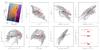 |
Fig. B.1 Correlation plots. Red dots are the face-on integrated values; gray dots are the original data shown throughout the main text. The first panel shows the lines along which the data are integrated. |
All Tables
Mean values (standard deviation between brackets) of several quantities in the several regions (η = I[ C ii ]/IFIR).
Results from Gaussian fit (points B–E with two components) to individual spectra with a spatial resolution of 15.9″ sampled at 7.55″.
All Figures
|
Fig. 1 [C ii] line-integrated intensity; points indicate positions where individual spectra are extracted for illustrative purposes (see Sect. 3.3). |
| In the text | |
|
Fig. 2 [C ii] line-integrated intensity convolved to 36″ resolution with selected regions (see Sect. 3.2) indicated. |
| In the text | |
|
Fig. 3 CO (1 − 0) line-integrated intensity convolved to 36″ resolution with selected regions (see Sect. 3.2) indicated. |
| In the text | |
|
Fig. 4 [C ii] channel maps from 8.0 km s-1 to 16.0 km s-1 in steps of dv = 0.5 km s-1 at 15.9″ resolution. The main-beam temperature Tmb is averaged over the step size dv. The first panel shows the line-integrated intensity. |
| In the text | |
|
Fig. 5 Different quantities with [C ii] emission in units of K km s-1 in contours: IFIR tracing the UV radiation field re-radiated in the FIR by dust particles, I8 μm tracing the UV radiation field by fluorescence of PAHs, ICO (1 − 0) tracing the molecular gas, τ160 tracing the dust column, IHα emitted by ionized gas, and, finally, the ratio I[ C ii ]/IFIR. All maps are convolved to 36″ spatial resolution and re-gridded to a pixel size of 14″, that of the SPIRE 500 μm map. |
| In the text | |
|
Fig. 6 Line spectra towards points A–I with average spectrum over the entire map (including H ii region) in the top left panel. Point A corresponds to the Horsehead PDR, points B to D are located in PDR1, points E and F lie in PDR2, point G represents the intermediate PDR front, point H is located in a region of little [C ii] emission, and point I represents PDR3. |
| In the text | |
|
Fig. 7 Results of our edge-on models described in Sect. 3.4. The panels show the gas temperature T (upper panels), IFIR, I[ C ii ], I[ C ii ]/IFIR, and ICO (1 − 0) (middle panels) and C+, C, and CO fractional abundances (lower panels) versus physical scale, for the gas densities nH = 3.0 × 103 cm-3,1.6 × 104 cm-3,4.0 × 104 cm-3 (left to right panels), and AV,los = 0.5, 2.5, and5.0. We note that the gas temperature does not vary with AV,los. |
| In the text | |
|
Fig. 8 Correlation plots extracted from the Orion B maps, convolved to a uniform resolution of 36″ and pixel size of 15″. Dark blue diamonds represent the CO-dark cloud, blue diamonds represent the CO clumps, red squares represent the Horsehead neck, triangles in different shades of green represent the PDRs (bright green is the Horsehead PDR), and yellow triangles represent the H ii region. Edge-on model predictions for selected gas densities are plotted as lines. Dashed lines are for AV,los = 2.5, with dark gray corresponding to a gas density of nH = 3.0 × 103 cm-3, medium gray to nH = 1.6 × 104 cm-3, and light gray to nH = 4.0 × 104 cm-3; dotted lines are the same but for AV,los = 5.0; the medium and light gray dash-dotted lines are for AV,los = 0.5, with nH = 1.6 × 104 cm-3 and nH = 4.0 × 104 cm-3, respectively. In panel f, the best fit is plotted as a line. |
| In the text | |
|
Fig. 9 Correlation plot of I[ C ii ]/IFIR versus ICO (1 − 0)/IFIR. Edge-on model predictions for selected gas densities are plotted as lines. Dashed lines are for AV,los = 2.5, with dark gray corresponding to a gas density of nH = 3.0 × 103 cm-3, medium gray to nH = 1.6 × 104 cm-3, and light gray to nH = 4.0 × 104 cm-3; dotted lines are the same but for AV,los = 5.0; the medium and light gray dash-dotted lines are for AV,los = 0.5, with nH = 1.6 × 104 cm-3 and nH = 4.0 × 104 cm-3, respectively. |
| In the text | |
|
Fig. 10 Correlation plot of I[ C ii ]/IFIR versus τ160. The plotted line corresponds to the relation expected from a simple face-on slab model, C/ (1 − exp( − τ160)); it is drawn such that it runs through the mean of I[ C ii ]/IFIR and τ160. |
| In the text | |
|
Fig. 11 Correlation plots of IFIR versus τ160, Td, and I8 μm, respectively. |
| In the text | |
|
Fig. 12 [C ii] spectra towards the H ii region, averaged over 156 (left) and 187 (right) pixels. The left panel represents the H ii region north of the Horsehead Nebula, the right panel represents the part south of the Horsehead Nebula. For the northern part, we obtain TP = 1.0 K, FWHM = 8.7 km s-1, and vP = 14.1 km s-1; for the southern part, a Gaussian fit yields TP = 0.7 K, FWHM = 5.2 km s-1, and vP = 11.2 km s-1. |
| In the text | |
|
Fig. 13 [C ii] spectra towards the Horsehead PDR and PDR1+2, averaged over 180 (left) and 3140 (right) pixels. Arrows indicate the positions of the [12C ii] line and the [13C ii] F = 2 − 1 and F = 1 − 1 lines (from left to right); the [13C ii] F = 1 − 0 line falls outside the spectral range of our map. |
| In the text | |
|
Fig. 14 Theoretical photoelectric heating efficiency of PAHs, clusters of PAHs, and very small grains is plotted against the ionization parameter γ = G0T0.5/ne (Bakes & Tielens 1994). We added the orange data points for the Horsehead PDR and PDR1. Blue data points are for the diffuse-ISM sight lines ζ Oph and o Per, and the PDRs Orion Bar and NGC 2023. Figure adapted from Tielens (2008). |
| In the text | |
|
Fig. 15 IRAC 8 μm image with lines A, B, C, and D indicated. |
| In the text | |
|
Fig. 16 IRAC 8 μm (PAH) intensity, Hα intensity, [C ii] and CO (1 − 0) line-integrated intensity, PACS 160 μm intensity, and SCUBA 850 μm intensity plotted in their respective native resolution along lines A, B, C, and D of Fig. 15 in their respective original spatial resolution. Multiply plotted values by 1.4 × 10⁻⁴, 2.9 × 10⁻³, 7.0 × 10⁻⁶, 1.6 × 10⁻⁹, 3,9 × 10⁻⁵, and 2.2 × 10⁻⁷, respectively, for I8 μm, IHα, I[ C ii ], ICO (1 − 0), I160 μm, and I850 μm, respectively, in erg s-1 cm-2 sr-1. |
| In the text | |
|
Fig. 17 Geometry of the L1630 molecular cloud surface. |
| In the text | |
|
Fig. 18 Original [C ii] image (line-integrated intensity) with Hα emission in contours (slightly smoothed). Contours from black to white: IHα = 0.5,1.0,2.0,3.0,4.0,5.0,6.0 × 10-3 erg s-1 cm-2 sr-1. |
| In the text | |
|
Fig. 19 Correlation plots for L1630 (Orion B) and OMC1 (Orion A); the OMC1 data are convolved to 25″ resolution, L1630 data to 36″ resolution. CO data are for the CO (1 − 0) line in L1630 and for the CO (2 − 1) line, divided by 8 (see Sect. 4.10), in OMC1. |
| In the text | |
|
Fig. B.1 Correlation plots. Red dots are the face-on integrated values; gray dots are the original data shown throughout the main text. The first panel shows the lines along which the data are integrated. |
| In the text | |
Current usage metrics show cumulative count of Article Views (full-text article views including HTML views, PDF and ePub downloads, according to the available data) and Abstracts Views on Vision4Press platform.
Data correspond to usage on the plateform after 2015. The current usage metrics is available 48-96 hours after online publication and is updated daily on week days.
Initial download of the metrics may take a while.