| Issue |
A&A
Volume 606, October 2017
|
|
|---|---|---|
| Article Number | A113 | |
| Number of page(s) | 14 | |
| Section | Extragalactic astronomy | |
| DOI | https://doi.org/10.1051/0004-6361/201630112 | |
| Published online | 23 October 2017 | |
The VIMOS Public Extragalactic Redshift Survey (VIPERS)
The distinct build-up of dense and normal massive passive galaxies⋆
1 INAF–Istituto di Astrofisica Spaziale e Fisica Cosmica Milano, via Bassini 15, 20133 Milano, Italy
e-mail: This email address is being protected from spambots. You need JavaScript enabled to view it.
2 INAF–Osservatorio Astronomico di Bologna, via Gobetti 93/3, 40129 Bologna, Italy
3 Institute of Physics, Jan Kochanowski University, ul. Swietokrzyska 15, 25-406 Kielce, Poland
4 INAF–Osservatorio Astronomico di Trieste, via G. B. Tiepolo 11, 34143 Trieste, Italy
5 INAF–Osservatorio Astronomico di Brera, via Brera 28, 20122 Milano, via E. Bianchi 46, 23807 Merate, Italy
6 Università degli Studi di Milano, via G. Celoria 16, 20133 Milano, Italy
7 Aix-Marseille Univ, CNRS, LAM, Laboratoire d’Astrophysique de Marseille, 13013 Marseille, France
8 INAF–Osservatorio Astrofisico di Torino, 10025 Pino Torinese, Italy
9 Laboratoire Lagrange, UMR7293, Université de Nice Sophia Antipolis, CNRS, Observatoire de la Côte d’Azur, 06300 Nice, France
10 Dipartimento di Fisica e Astronomia, Alma Mater Studiorum Università di Bologna, viale Berti Pichat 6/2, 40127 Bologna, Italy
11 National Centre for Nuclear Research, ul. Hoza 69, 00-681 Warszawa, Poland
12 INFN, Sezione di Bologna, viale Berti Pichat 6/2, 40127 Bologna, Italy
13 Department of Astronomy & Physics, Saint Mary’s University, 923 Robie Street, Halifax, Nova Scotia, B3H 3C3, Canada
14 Aix-Marseille Université, Jardin du Pharo, 58 bd Charles Livon, 13284 Marseille Cedex 7, France
15 IRAP, 9 Av. du Colonel Roche, BP 44346, 31028 Toulouse Cedex 4, France
16 Astronomical Observatory of the Jagiellonian University, Orla 171, 30-001 Cracow, Poland
17 School of Physics and Astronomy, University of St Andrews, St Andrews KY16 9SS, UK
18 INAF – Istituto di Astrofisica Spaziale e Fisica Cosmica Bologna, via Gobetti 101, 40129 Bologna, Italy
19 INAF – Istituto di Radioastronomia, via Gobetti 101, 40129, Bologna, Italy
20 Aix-Marseille Univ, Univ Toulon, CNRS, CPT, 13288 Marseille, France
21 Dipartimento di Matematica e Fisica, Università degli Studi Roma Tre, via della Vasca Navale 84, 00146 Roma, Italy
22 INFN, Sezione di Roma Tre, via della Vasca Navale 84, 00146 Roma, Italy
23 INAF–Osservatorio Astronomico di Roma, via Frascati33, 00040 Monte Porzio Catone (RM), Italy
24 Department of Astronomy, University of Geneva, ch. d’Ecogia 16, 1290 Versoix, Switzerland
25 Institute for Astronomy, University of Edinburgh, Royal Observatory, Blackford Hill, Edinburgh EH9 3HJ, UK
Received: 22 November 2016
Accepted: 19 May 2017
Abstract
We have used the final data from the VIPERS redshift survey to extract an unparalleled sample of more than 2000 massive ℳ≥1011 M⊙ passive galaxies (MPGs) at redshift 0.5≤z≤1.0, based on their NUVrK colours. This has enabled us to investigate how the population of these objects was built up over cosmic time. We find that the evolution of the number density depends on the galaxy mean surface stellar mass density, Σ. In particular, dense (Σ≥2000 M⊙ pc-2) MPGs show a constant comoving number density over this redshift range, whilst this increases by a factor of approximately four for the least dense objects, defined as having Σ < 1000 M⊙ pc-2. We estimated stellar ages for the MPG population both fitting the spectral energy distribution (SED) and through the D4000n index, obtaining results in good agreement. Our findings are consistent with passive ageing of the stellar content of dense MPGs. We show that at any redshift the less dense MPGs are younger than dense ones and that their stellar populations evolve at a slower rate than predicted by passive evolution. This points to a scenario in which the overall population of MPGs was built up over the cosmic time by continuous addition of less dense galaxies: on top of an initial population of dense objects that passively evolves, new, larger, and younger MPGs continuously join the population at later epochs. Finally, we demonstrate that the observed increase in the number density of MPGs is totally accounted for by the observed decrease in the number density of correspondingly massive star forming galaxies (i.e. all the non-passive ℳ≥1011 M⊙ objects). Such systems observed at z ≃ 1 in VIPERS, therefore, represent the most plausible progenitors of the subsequent emerging class of larger MPGs.
Key words: galaxies: elliptical and lenticular, cD / galaxies: evolution / galaxies: formation / galaxies: high-redshift
Based on observations collected at the European Southern Observatory, Cerro Paranal, Chile, using the Very Large Telescope under programs 182.A-0886 and partly 070.A-9007. Also based on observations obtained with MegaPrime/MegaCam, a joint project of CFHT and CEA/DAPNIA, at the Canada-France-Hawaii Telescope (CFHT), which is operated by the National Research Council (NRC) of Canada, the Institut National des Sciences de l’Univers of the Centre National de la Recherche Scientifique (CNRS) of France, and the University of Hawaii. This work is based in part on data products produced at TERAPIX and the Canadian Astronomy Data Centre as part of the Canada-France-Hawaii Telescope Legacy Survey, a collaborative project of NRC and CNRS. The VIPERS web site is http://www.vipers.inaf.it/
© ESO, 2017
1. Introduction
One of the most debated issues in modern astrophysics concerns the formation and evolution of passive galaxies (PGs). From a theoretical point of view, it is still debated whether these systems assembled their stellar mass mostly by mergers (e.g. Naab et al. 2009; Qu et al. 2017), or through other “in-situ” processes, such as the accretion of clumps through the disc (e.g. Dekel et al. 2009).
From an observational point of view, deep imaging and dynamical studies have shown that the PGs already in place at z ~ 2 have average sizes smaller than comparable galaxies at the current epoch (Cimatti et al. 2004; Daddi et al. 2005; Trujillo et al. 2006; Longhetti et al. 2007; van Dokkum et al. 2008; Cimatti et al. 2008; van der Wel et al. 2008; Bezanson et al. 2009; Cassata et al. 2011; Belli et al. 2014). For example, high-z PGs with ℳ~1011 M⊙ have an average effective radius of Re~1–2 kpc with a mean stellar mass density Σ = ℳ/(2πRe2) of 2000 ≲ Σ ≲ 6000 M⊙ pc-2 while local PGs with similar stellar mass have Re~5 kpc and Σ~1000 M⊙ pc-2 (e.g. Shen et al. 2003; Kauffmann et al. 2003)
These data have been widely interpreted within a two-phases scenario (commonly called “inside-out”). During the first phase, a highly dissipative process (e.g. a gas-rich merger; Hopkins et al. 2008) or in situ accretion of cold streams (Kereš et al. 2005; Dekel et al. 2009) forms the compact passive cores we observe at high redshift. Subsequently, as time goes by, this compact galaxy assembles an external and low-density halo through many dry minor mergers. The overall effect of these mergers is to increase the galaxy radius till it matches the typical dimension of a local PG (e.g. Naab et al. 2007, 2009; Hilz et al. 2013; van Dokkum et al. 2008).
This scenario is supported by the drastic decrease (more than two orders of magnitude) in the number density of compact PGs over time, observed in some studies (e.g. Cassata et al. 2013; van der Wel et al. 2014). However, other analyses have found a very mild decrease (e.g. Poggianti et al. 2013b; Valentinuzzi et al. 2010), or even a constant number density evolution (e.g. Damjanov et al. 2014, 2015; Saracco et al. 2010; Gargiulo et al. 2016). A good summary of the different results is provided in Damjanov et al. (2014) and Gargiulo et al. (2016) (see their Figs. 7 and 2 respectively). This disagreement casts doubts on the necessity of a size-growth for individual compact PG. Differences in the selection criteria of passive galaxies (morphology vs. colour-colour diagram vs. specific star formation rate [sSFR] cut), in the selection of its dense sub-population (e.g. cut at constant Re, Σ, or at 1–2σ below the size-mass relation (SMR)), and in the rest-frame waveband used to derive the effective radius, have been found to play a major role in the observed discrepancy (Gargiulo et al. 2016). This evidence highlights the necessity of a homogeneous analysis over the cosmic time to draw robust conclusions on this relevant issue.
Evidence shows that in conjunction with an increase in the mean radial size of PGs by a factor of ~4 from z ~ 1.5−2 to z = 0, the number of PGs per unit volume increases by a factor of approximately ten (e.g. Pozzetti et al. 2010; Ilbert et al. 2010; Brammer et al. 2011). If the number density of high-z dense PGs drastically falls, as observed by some authors, because they increase their size, their contribution to the whole population of local PGs would have to be less then 10%, since high-z PGs are ten times less numerous than local PGs. Consequently, the majority of local PGs would need to have formed through a mechanism other than the inside-out model. On the other hand, if all local PGs were assembled according to the inside-out model, new compact PGs would need to form continuously at z< 1.5−2 and then increase their sizes in order to sustain the numerical growth of the whole population. This picture could help to explain the works that show a mild or null evolution in the number density of compact PGs. However, if this were the case, further evidence would be expected: the age of dense PGs should not evolve significantly over time, since this sub-population would be constantly refreshed by new galaxies. In fact, if the number density of compact PGs is confirmed to evolve slowly, a third hypothesis is also viable: compact PGs might passively age and the increase both in mean Re and in the number of PGs over the time could then mostly be due to the fact that galaxies that quench at later epoch are larger (e.g. Valentinuzzi et al. 2010; Cimatti et al. 2008; Carollo et al. 2013). It is common habit to refer to this last scenario as progenitor bias (e.g. Franx & van Dokkum 1996). In this picture the age of the stellar population of compact PGs over cosmic time should be consistent with passive evolution. Thus, valuable insights into the build up of the PG population can be gained by studying the evolution of the number density and the age of the stellar population together.
In this context, massive (ℳ>1011 M⊙) PGs (MPGs) deserve particular attention. These systems are expected to evolve mainly through (dry) mergers (e.g. Hopkins et al. 2009; De Lucia & Blaizot 2007). If this is the case, in this mass range we should detect a stronger signal of the size-growth with respect to a lower mass range. So far, because MPGs are extremely rare, there have been very few studies that have investigated the combined evolution of the number density and of the age of MPGs as a function of their compactness (Carollo et al. 2013; Fagioli et al. 2016). Carollo et al. (2013) found that the number density of massive quiescent and elliptical galaxies with Re< 2.5 kpc decreases by about 30% from z~1 to z~0.2 and that their U−V colours are consistent with passive evolution. They concluded that the driving mechanism for the average size-growth of the whole population is the appearance at later epochs of larger quiescent galaxies. More recently, Fagioli et al. (2016, hereafter F16) analysed the spectroscopic properties of ~500 MPGs (defined as galaxies with absent or very weak emission lines and no MIPS detections) at 0.2 <z< 0.8 in the zCOSMOS-bright 20 K catalogue (Lilly et al. 2007). From the analysis of stacked spectra of small and large MPGs, they dated the stellar content of these groups and found that the two sub-populations have similar ages. The authors concluded that, in this mass regime, the size growth of individual galaxies through dry mergers is the most likely explanation for the increase in the mean effective radius of the whole population. A recent analysis by Zahid et al. (2016) on the physical properties of compact post starburst galaxies at 0.2<z<0.8 with ℳ>1011 M⊙ provides new insights. On the basis of both their number density and of their ages, which have been found to be <1 Gyr, the authors suggest that this class of objects are the progenitors of compact quiescent galaxies. They conclude that a substantial fraction of dense quiescent galaxies at z<0.8 are newly formed.
Despite the efforts and improvements of recent years, the overall picture is far from clear. What is still missing is a homogeneous analysis of the number density and stellar population age at z~0.8, that is over the redshift range where less compact MPGs start to dominate the Universe (e.g. Cassata et al. 2010, 2013). For this goal to be achieved the following three requirements must be met: significant samples of MPGs at different redshifts, in order to have good statistics in each redshift and Σ bin; a large volume to minimise the effect of the cosmic variance (which is known to affect the COSMOS field); robust estimates of the ages of stellar populations.
The VIMOS Public Extragalactic Redshift Survey (VIPERS) represents an ideal benchmark for this kind of study. Despite the fact galaxies with ℳ > 1011 M⊙ are rare, the wide area (~16 effective deg2 over the W1 and W4 CFHTLS fields, more details in Sect. 2) and high sampling rate of the survey (~40%) result in a sample of ~2000 MPGs with spectroscopic redshifts over the redshift range 0.5≤z ≤ 1.0 (see Sect. 2). The unprecedented quality of statistics over this redshift range allows us to study the evolution of the number density of MPGs as a function of Σ (see Sect. 4). Using D4000n as a spectroscopic diagnostic and by fitting the spectral energy distribution (SED) we constrained the age of the stellar population of MPGs as a function both of z and Σ (Sect. 5). This information, together with the evolution of the number density, allowed us to put constraints on the mass accretion scenarios and on the origin of new MPGs (Sect. 6). We summarise all of our results in Sect. 7. Throughout the paper we adopt the Chabrier (2003) initial mass function (IMF) and a flat cosmology with ΩM = 0.3, ΩΛ = 0.7 and H0 = 70 km s-1 Mpc-1. Magnitudes are in the AB system. Effective radii are circularised, meaning that  , where a and b are the semi-major and semi-minor axis of the isophote containing half of the total light, respectively.
2. Data
2.1. The VIPERS project
In this work we analyse a beta version of the final public data release of VIPERS. The data set used here is almost identical to the publicly released PDR-2 catalogue (Scodeggio et al. 2017), with the exception of a sub-set of a few redshifts (mostly at z> 1.2), which were revised close to the release date. This has no effect on the analysis presented here. VIPERS has measured redshifts for 89 128 galaxies to iAB = 22.5, distributed over a total area of 23.5 deg2. This reduces to an effective area of 16.3 deg2 once detector gaps and masked areas such as those with bright stars are accounted for. Spectroscopic targets were selected in the W1 and W4 fields of the Canada-France-Hawaii Telescope Legacy Survey (CFHTLS) Wide. The star-galaxy classification criterion was defined after extensive tests on the VVDS survey (Le Fèvre et al. 2005; Garilli et al. 2008, 2014). In detail, stars were classified as those systems with i) iAB<21 and rh<μrh + 3σrh or ii)  21, rh<μrh + 3σrh and log 10(
 ) <log 10(
 , where rh is the half-light radius as derived from SExtractor (Bertin & Arnouts 1996), μrh and σrh are the mean and standard deviation of the rh distribution, while and
  are the χ2 of the SED fitting applied to the ugriz CFHTLS photometry. A robust colour-colour pre-selection in the ugri plane was used to identify galaxies at z>0.5. In particular, among all of the objects classified as galaxies, were flagged as spectroscopic target those with:
  (1)Spectroscopic observations were carried out with VIMOS at the VLT using the low-resolution red grism (R~220), which covers the wavelength range 5500–9500 Å. The rms error of the measured redshifts has been estimated to be σz(z) = 0.00054 × (1 + z) (Scodeggio et al. 2017). In the same paper, a complete description of the PDR-2 data release can be found, while more information on the original survey design and data reduction procedures are found in Guzzo et al. (2014) and Garilli et al. (2014).
For each galaxy of the VIPERS spectroscopic sample, physical properties such as the multi-band luminosity and the total stellar mass were derived through the SED fit. The photometric multi-wavelength coverage combines improved ugriz-bands photometry based on the T0007 release of the CFHTLS1 and Ks-band observations from the VIPERS Multi-Lambda Survey (VIPERS-MLS2, Moutard et al. 2016a) or, when available, from the VISTA Deep Extragalactic Observations (VIDEO; Jarvis et al. 2013) survey (more details in Davidzon et al. 2013, 2016; Moutard et al. 2016b).
The fit was performed with the Hyperzmass software (Bolzonella et al. 2000). The template libraries adopted in the fit procedure are fully described in Davidzon et al. (2013) and are based on Bruzual & Charlot (2003) models, with exponentially declining star formation history (∝e− t/τ, where τ is the timescale of the star formation), τ in the range [0.1–30] Gyr, sub-solar (0.2 Z⊙) and solar metallicity, and the Chabrier (2003) IMF. The impact of dust extinction on the input galaxy templates was modelled according to two different prescriptions (Calzetti et al. 2000; Prevot et al. 1984) with the extinction parameters AV ranging from 0 (no dust) to 3 mag.
The structural parameters (effective radius Re, Sersic index n) for ~85% of the VIPERS sources were derived with GALFIT (Peng et al. 2002) fitting the i-band CHFTLS-Wide images with a 2D-psf convolved Sersic profile (Krywult et al. 2017). The CFHTLS public images have a pixel-scale of ~0.187′′/px and the full width at half maximum (FWHM) of point-like sources varies from ~0.5′′ to 0.8′′ in the i band. To control the variability of the PSF over the wide CCD area of CFHTLS images (1° × 1°) Krywult et al. (2017) selected a set of ~2000 stars uniformly distributed over each field and modelled their profiles using a 2D Chebychev approximation of the elliptical Moffat function. This approach allowed the PSF to be successfully described over ~95% of the whole VIPERS area. Only regions without bright and unsaturated stars, or at the edge of the images (hereafter bad PSF regions) were excluded. Since these regions are well defined, we have removed them from our analysis. Taking this into consideration the effective final area we used in this analysis is ~14 deg2.
Krywult et al. (2017) tested the reliability of Re and n derived from ground-based CFHTLS images. They found that the typical effective galaxy radius is recovered within 4.4% and 12% for 68% and 95% of the total sample respectively. We refer to their paper for further details.
2.2. The sample of massive passive galaxies
From the VIPERS spectroscopic catalogue we selected all galaxies with highly accurate redshift measurements, i.e. with quality flag 2 
 9.5 (a confidence level >95%; 75 479 galaxies in the W1+W4 field). We defined galaxies as passive on the basis of their location in the rest-frame colour NUV-r vs. r-K diagram, which is a powerful alternative to the UVJ diagram (Williams et al. 2009) to properly identify passive galaxies (for more details see Arnouts et al. 2013; Davidzon et al. 2016; Moutard et al. 2016a,b). Following Davidzon et al. (2016), we defined quiescent galaxies as those satisfying the following conditions:
 ![Mathematical equation: \begin{eqnarray} &&{\rm NUV} - {r} > 3.75, \\[2mm] &&{\rm NUV} - {r} > 1.37 \times ({r} - {K}) + 3.2, \\[2mm] &&{r} - {K} < 1.3. \end{eqnarray}](/articles/aa/full_html/2017/10/aa30112-16/aa30112-16-eq92.png) Among all galaxies satisfying these three conditions (7606 in W1 and 3939 in W4, respectively) ~95% have sSFR<10-11 yr-1. From the quiescent population we selected the sub-sample with ℳ ≥ 1011 M⊙ (hereafter MPGs; 1905 galaxies in the W1 field, and 902 in W4) which is complete up to z = 1.0 (see e.g. Davidzon et al. 2013; Fritz et al. 2014; Davidzon et al. 2016). Below z = 0.5, VIPERS is highly incomplete due to the ugri colour cuts imposed in the selection of spectroscopic targets. Thus the following analysis is limited to the redshift range 0.5z1.0. Finally, we excluded from our analysis galaxies that are in bad PSF regions (see Sect. 2.1). These further cuts leaves us with a sample of 2022 MPGs.
Among all galaxies satisfying these three conditions (7606 in W1 and 3939 in W4, respectively) ~95% have sSFR<10-11 yr-1. From the quiescent population we selected the sub-sample with ℳ ≥ 1011 M⊙ (hereafter MPGs; 1905 galaxies in the W1 field, and 902 in W4) which is complete up to z = 1.0 (see e.g. Davidzon et al. 2013; Fritz et al. 2014; Davidzon et al. 2016). Below z = 0.5, VIPERS is highly incomplete due to the ugri colour cuts imposed in the selection of spectroscopic targets. Thus the following analysis is limited to the redshift range 0.5z1.0. Finally, we excluded from our analysis galaxies that are in bad PSF regions (see Sect. 2.1). These further cuts leaves us with a sample of 2022 MPGs.
For each of these galaxies we need to derive its mean stellar mass density Σ. In the redshift range 0.5z1.0, the i-band filter covers the spectral region across the 4000 Å break. In particular, it samples the ~V-band (5000 Å) rest-frame at z = 0.5 and the ~U-band (3500 Å) rest-frame at z = 1.0. Given the presence of radial colour variations in passive galaxies both at high and low redshift (see e.g. La Barbera & de Carvalho 2009; Saglia et al. 2010; Gargiulo et al. 2012; Guo et al. 2011), the variation of the rest-frame band used to derive Re can induce a spurious trend in the evolution of the radius with redshift. To quantify this bias, the structural parameters for the whole W4 field (and for ~40% of the W1 field) have been derived in the r-band (FWHM~0.8′′, ~U-band rest-frame at z ≲ 0.8). Figure 1 shows the ratio between the Re of MPGs in the r and i band (Re,r/Re,i) as a function of their Re,i at z<0.8. For a rigorous analysis, we derived the relations in three finer redshift bins (0.5z<0.6, 0.6z<0.7, 0.7z<0.8). The general trend, as derived from the best-fit relations, is that for MPGs Re,i<Re,r, meaning that the internal regions are redder than the outskirts, as expected for passive systems (e.g. La Barbera & de Carvalho 2009). For the smallest galaxies the difference between the two radii can be up to ~20%. We note that a portion of MPGs (especially at large Re) has Re,i>Re,r, suggesting the presence of a blue core. However, a detailed study on the internal colour variation in MPGs is beyond the scope of this paper.
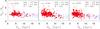 |
Fig. 1 Ratio between the effective radius in r band (Re,r) and the effective radius in i band (Re,i) as a function of Re,i for MPGs in three bins of redshift as indicated in the top left corner of each plot. In the three panels, the solid blue lines are the best fit relations derived with a sigma-clipping algorithm. Dashed blue lines set the 1σ deviation. The typical dimension of half of the PSF-FWHM of both i-band and r-band images is indicated in the top right corner of each plot with also the number of objects. Open red circles are galaxies at >3σ from this fit. |
Given the evidence presented in Fig. 1, in the derivation of Σ we referred to the effective radius in the r band for MPGs at z<0.8, and to Re in the i band for those at z≥0.8. By doing this, we were able to approximately sample the same U band rest-frame over the whole redshift range we probe. For those MPGs at z<0.8 without an Re,r estimate (mostly in the W1 field), we estimated Re,i using the relations of Fig. 1. We checked that the addition of galaxies with Re,r derived from Re,i does not change the Σ distribution of the sample of MPGs at z< 0.8.
In Fig. 2 we show the fraction of MPGs with available and reliable structural parameters for W1 and W4 fields and for the total area as a function of redshift.
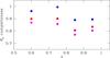 |
Fig. 2 Fraction of MPGs with available Re in the W1 field (magenta filled points), in the W4 field (blue filled points) as a function of z. At z<0.8, MPGs with Re derived from i-band images are included. Red filled points indicate the completeness for the W1+W4 field. |
Overall, ~85% of MPGs in the two fields have a reliable Re. For ~15% of MPGs structural parameters are not available since in some cases we are unable to fit the surface brightness profile. This is either because the algorithm does not converge, mostly because of very close companions, or the best-fit values of n <0.2 are unphysical (see Krywult et al. 2017). Once these objects have been excluded, the final sample of MPGs with reliable Re (hence Σ) in the redshift range 0.5–1.0 is composed of 1758 galaxies.
3. The size mass relation of MPGs in VIPERS for 0.5 < z < 1.0
In Fig. 3 we show the SMR for the VIPERS MPGs in the lowest and highest redshift bins of our sample, that is 0.5z<0.7 and 0.9z1.0. We fitted a SMR of MPGs of the form log Re = αlog (ℳ/1011) + β adopting an ordinary least squares fit without taking into account errors on Re. The best-fit results are reported in Table 1. We also added the result for the intermediate bin (0.7≤z<0.9).
Best-fit values (α, β) of the size mass relation log Re = αlog (ℳ/1011) + β of VIPERS MPGs.
In agreement with previous studies (e.g. Damjanov et al. 2011; van der Wel et al. 2014), we find that at 1σ there is almost no evolution of the slope of the SMR with time. However, there is an offset among the zero-points. On average, at fixed stellar mass, MPGs at ⟨ z ⟩ = 0.6 have Re~1.25 larger than those at z = 1.0. This increase shows that the growth in the mean Re of the passive population is gradual and continuous, extending out to z<1. The increase in Re is in agreement with what has been found by other authors. Damjanov et al. (2011), for a sample of early-type galaxies at 0.2<z<2.7, found ⟨ Re ⟩ ∝ (1 + z)− 1.62 ± 0.34, independently of the stellar mass of the galaxy, that is an increase by a factor ~1.4 ± 0.1 in the redshift range 0.6–1.0. Similarly, Williams et al. (2010) found ⟨ Re ⟩ ∝ (1 + z)-1.3 for passive galaxies (UVJ selected) with ℳ>1011 M⊙ which results in an increase of a factor ~1.3 in our redshift range. From the analysis of passive galaxies (UVJ colour selected) with ℳ>2 × 10¹⁰ M⊙, van der Wel et al. (2014) found ⟨ Re ⟩ ∝ (1 + z)-1.48 over the redshift range 0<z<3, still in fair agreement with our results.
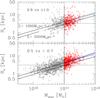 |
Fig. 3 Size-mass relation of passive VIPERS galaxies (grey open + red open points) in the two extreme redshift bins of our analysis (0.5 |
In Fig. 4 we directly show the distribution of Re of MPGs in the same redshift bins as Fig. 3. Although the two distributions are significantly different (KS test probability <10-8), the figure shows that they cover the same range of Re. This suggests that the population of compact MPGs does not totally disappear with cosmic time. In the next section we will quantify this qualitative trend by estimating the comoving number density of MPGs with different Σ.
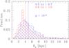 |
Fig. 4 Distribution of the effective radius for MPGs in our lowest (blue histogram) and highest (red histogram) redshift bins. The solid lines indicate the median values of the two distributions. The probability p that the two distributions are extracted from the same parent sample are reported in the label. |
4. The number density of MPGs in VIPERS as a function of redshift and mean stellar mass density
In order to derive the number density of the MPGs as a function of Σ we subdivided our sample into a “high-Σ sample”, consisting of galaxies with Σ≥2000 M⊙ pc-2, an “intermediate-Σ sample”, consisting of galaxies with 1000<Σ2000 M⊙ pc-2, and a “low-Σ sample” consisting of galaxies with Σ<1000 M⊙ pc-2. The choice of a cut at 2000 M⊙ pc-2 was determined by the characteristics of the CFHTLS images. In Fig. 3, the horizontal solid lines indicate half of the FWHM of the PSF. We note that all the MPGs with Re below half the FWHM of the images, at any redshift, have Σ ≳ 2000 M⊙ pc-2. Adopting this cut ensures that all galaxies with radii lower than the resolution of the image (i.e. galaxies for which Re could be overestimated), are in the same Σ bin and do not spuriously contaminate other bins. We stress that this is a conservative choice. Effective radii are derived by deconvolving the data for the real PSF of the images. At the typical S/N of our galaxies, measurements of Re lower than the image resolution are robust as shown in the Appendix of Krywult et al. (2017).
In Table 2, we list the total number of galaxies in each bin of stellar mass density, and for each redshift bin. Their sum is smaller than the total number of galaxies (Col. 1, Table 2) since for a fraction of galaxies we do not have a reliable estimate of their structural parameters (see Sect. 2.2).
Total number of massive quiescent galaxies and of the high-Σ sample, intermediate-Σ sample, and low-Σ sample in the four redshift bins 0.5z<0.7, 0.7<z0.8, 0.8<z0.9, 0.9<z1.0.
The VIPERS final sample (and hence our final sample of MPGs) suffers from three sources of incompleteness. These are the target sampling rate (TSR), the success sampling rate (SSR), and the colour sampling rate (CSR). The TSR is given by the ratio of galaxies effectively observed with respect to the photometric parent sample. The SSR is the fraction of spectroscopically observed galaxies with a redshift measurement. The CSR takes into account the completeness due to the colour selection of the survey. These statistical weights (hereafter TSR(i), SSR(i), CSR(i)) depend on the magnitude of the galaxy, on its redshift, colour, and angular position. They have been derived for each galaxy in the full VIPERS sample (for a detailed description of their derivation see Garilli et al. 2014; Scodeggio et al. 2017). In the derivation of the number density, we weighted each MPG i in our sample by the quantity w(i) = 1/(TSR(i)*SSR(i)*CSR(i)).
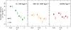 |
Fig. 5 Number densities for massive passive galaxies with Σ≥2000 M⊙ pc-2 (right panel, dark red symbols), 1000≤Σ<2000 M⊙ pc-2 (central panel, orange symbols), and Σ<1000 M⊙ pc-2 (left panel, green symbols), for the W1 field (filled circles) and W4 one (open circles). Number densities for the W4 field are shifted in redshift to better visualize them. The error bars correspond to 1σ. |
Beside these sources of incompleteness, a fraction of MPGs is lacking reliable structural parameters. In Fig. 2 we show this fraction as a function of redshift. We checked whether the galaxies without structural parameters belong mainly to a sub-population of galaxies of a given Σ. To address this issue, we compared the fraction of high-, intermediate- and low-Σ MPGs in different redshift bins (which have different levels of completeness). We did not find any significant variation between redshift bins. Given that there is no dependence of the lack of structural parameters on Σ (or vice versa), we corrected the number densities of MPGs for this source of incompleteness, using the values in Fig. 2.
In Fig. 5 we show the number density of MPGs as a function of redshift and mean stellar mass density, both in the W1 and W4 fields. Error bars were derived taking into consideration Poisson fluctuations, and the uncertainties on the Re estimates. To consider this last source of uncertainty, we computed the standard deviation σ(z, Σ) over 100 number density estimates obtained by replacing for each galaxy the effective radius Re with a value randomly drawn from a Gaussian distribution with mean value Re and standard deviation the typical error on Re (i.e. 0.05 Re, see Sect. 2.1).
The estimates of the number density in the W1 and W4 fields are in very good agreement, indicating that the wide area of VIPERS reduces the effect of cosmic variance even for the most massive galaxy sample. This result is in agreement with the expected cosmic variance of ~10% derived for VIPERS massive galaxies in Davidzon et al. (2013). In Fig. 6 we report the number density of MPGs as a function of Σ (plus the number density for the whole population of MPGs) in the total VIPERS area (W1 + W4). Error bars are derived as described above.
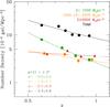 |
Fig. 6 Number density of MPGs with different mean stellar mass density in VIPERS field as a function of the redshift. Dark red triangles refer to high-Σ MPGs, orange circles refer to intermediate-Σ MPGs, and green squares to low-Σ MPGs. Black circles show the number density for the total sample of MPGs. Number densities for the three sub-populations are shifted in redshift to better visualize them. The error bars correspond to 1σ. We fitted the data with a power law and solid lines are the best-fit relations. |
The evolution of the number density of the whole population of MPGs is well fitted by a function ρ ∝ (1 + z)α, with α = −3.3 ± 0.9. In the ~2.5 Gyr from z = 1.0 to z = 0.5, the number density of MPGs increases by a factor ~2.5. Similarly, we fitted the number density evolution of the three sub-populations with a power law, and found α = −5.0 ± 0.4 for low-Σ MPGs, α = −1.8 ± 0.7 for intermediate-Σ MPGs and α = −0.7 ± 0.9 for high-Σ MPGs. We find that the evolution of the number density strongly depends on the mean stellar mass density of the system. In particular, the lower the mean stellar mass density, the faster the evolution. The number density of the densest MPGs is approximately constant over the whole redshift range, while the number density of less dense MPGs constantly increases with time by a factor of approximately four.
Figure 6 shows that we are looking at a crucial moment in the build up of the MPG population, that is when less compact galaxies, which constitute the bulk of the local MPG population, start to dominate. In fact, at z>0.8, the population of MPGs is composed in equal parts of high, intermediate and low-Σ galaxies. At lower redshift, the contribution of low-Σ MPGs steadily increases. At z = 0.5 compact quiescent galaxies account for just ~15% of the whole population. Less compact systems, on the other hand, account for more than half of the whole population. This result is in agreement with the analysis by Cassata et al. (2011) who found that normal (i.e. less dense) passive (sSFR<10-11 yr-1) and elliptical galaxies with 1010<ℳ ≲ 1011.5 M⊙ start to become the dominant sub-population at z~0.9.
Our results are in good agreement also with Carollo et al. (2013) who found that the number density of passive (sSFR< 10-11 yr-1) and elliptical galaxies with ℳ > 1011 M⊙ and Re<2.5 kpc decreases by ~30% in the 5 Gyr between z~1 and z~0.2. Damjanov et al. (2015) found an almost constant number density over the redshift range 0.2<z< 0.8 for colour selected passive compact galaxies with ℳ>8 × 10¹⁰ M⊙. Gargiulo et al. (2016) found ρ(z) ∝ (1 + z)0.3 ± 0.8 for a sample of morphologically selected elliptical dense galaxies ( M⊙ pc-2) with ℳ > 1011 M⊙ in the redshift range 0 <z<1.6, consistent with our results. Cassata et al. (2013) found a very mild decrease of compact galaxies (1σ below the local SMR), and a mild increase in the number density of normal galaxies (consistent at 1σ with the local SMR) from z~1 to z~0.5, in qualitative agreement with our results. However, they found that the number density of ultra-compact galaxies (0.4 dex smaller than local SDSS counterparts of the same mass) dramatically decreases. A detailed comparison with our results is not possible given the different selection of the samples. Nonetheless, we verified that the constant trend for high-Σ MPGs we show in Fig. 6 is not related to the adopted cut Σ = 2000 M⊙ pc-2. We estimated the number density for the sub-sample of MPGs with Σ>3000 M⊙ pc-2 and Σ>4000 M⊙ pc-2 and found α = −0.5 ± 1.4 and α = −1.3 ± 1.5. These results are consistent at 1σ with the results we found for the high-Σ sub-population.
If the global population of dense passive galaxies were to evolve in size, then in order to maintain a constant number density of the compact sub-population over cosmic time, new dense galaxies would have to appear at lower redshift. In particular, the timescale of the size-growth mechanisms and that of the appearance of new dense massive quiescent galaxies would need to be very similar (e.g. Carollo et al. 2013). The other possibility is that the dense MPGs passively evolve without changing their structure. One way to discriminate between these two possibilities is to study of the age of the stellar population as a function of the mean stellar mass density.
5. The stellar population age of MPGs as a function of the redshift and mean stellar mass density
For any individual galaxy, we constrained its stellar population age fitting the photometric SED (ageSED). Since we are aware of the age-metallicity degeneracy which can affect the SED fitting estimates, we adopted the independent measurements of D4000n to validate our conclusions.
The D4000n index (Balogh et al. 1999) is an age sensitive spectral feature (Kauffmann et al. 2003) defined as the ratio between the continuum flux densities in the blue region [3850–3950] Å and red region [4000–4100] Å across the 4000 Å break: 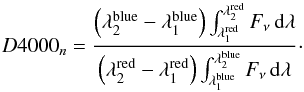 (5)A complete description of the D4000n measurements for VIPERS galaxies is presented in Garilli et al. (2014). Siudek et al. (2017), using stacked spectra, have already investigated the star formation epoch of all of VIPERS passive galaxies through the analysis of both the D4000n and the Hδ Lick index. The authors selected passive galaxies using an evolving cut in the rest-frame U−V colour and found that, over the full analysed redshift and stellar mass range (0.4<z<1.0 and 10<log (ℳ/M⊙) < 12, respectively), the D4000n index increases with redshift, while Hδ gets lower. Here, instead of looking for trends of D4000n with stellar mass and z, we focused our analysis on a given stellar mass bin, and investigate within this bin the trend of D4000n with Σ and z. We selected MPGs with the error on D4000n smaller than 8% in order to restrict the analysis to galaxies with a highly accurate estimate of D4000n. This criterion further reduces the sample by ~10%, but does not alter the distribution in Σ. Figure A.1 shows how the conversion of the D4000n into a stellar population age depends both on metallicity Z and on the timescale τ of the star formation of the galaxy (we report the trend in the case of an exponentially declining star formation history). Given the spectral coverage and resolution of our spectra, we can accurately measure D4000n for each individual galaxy but conversely we cannot constrain either Z or the timescale. Instead of making a blind assumption of Z and τ, we exploited the capabilities of our spectroscopic+photometric dataset. We firstly constrained the evolution of stellar population ages as derived from SED fitting. Starting from the best-fit models of the SED, we derived the mean value of AgeSED(z, Σ) for MPGs in each bin of z and Σ and investigated its evolution over the cosmic time. Since the estimate of the Age from the SED fitting could be biased by the age-metallicity degeneracy, we compared the predictions we obtained with the independent measurements of stellar population ages obtained by the spectroscopic index D4000n. In details, together with AgeSED(z, Σ), we derived ZSED(z, Σ), and τSED(z, Σ) from the best-fit models of the SED. Using low-resolution (lr) BC03 models (i.e. the same as those used to perform the SED fitting), we derived the D4000n corresponding to these mean values, D4000n,SED(z, Σ), and compared these estimates with the mean value of the distribution of D4000n of all of the MPGs in that bin of z and Σ. For simplicity we focus this part of our analysis on the two extreme Σ sub-populations, the low-Σ and high-Σ MPGs. Results for intermediate-Σ MPGs are in between.
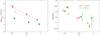 |
Fig. 7 Left panel: mean stellar population ages of MPGs as derived from the SED fitting as a function of redshift and mean stellar mass density for high- and low-Σ MPGs (filled points). The colour and symbols code is the same as in Fig. 6. Error bars indicate the error on the mean. Points refer to the redshift bins 0.5 |
In Fig. 7 filled points show the mean values of AgeSED and the mean value of D4000n (left and right panels, respectively) of low-Σ (green filled squares) and high-Σ (dark red triangles) MPGs. Error bars indicate the error on the mean. The left panel of Fig. 7 shows that for high-Σ MPGs the evolution of the stellar population ages derived from the SED fitting is consistent with a passive evolution of the population. In fact, their AgeSED increases by ~2 Gyr during the 1.8 Gyr of evolution between z = 0.95 and 0.6. At any redshift, the mean value of the timescale of star formation τ, as constrained by the SED fitting, is ~0.4 Gyr, and the best-fit models have a mean Z~0.5 ± 0.3 Z⊙3. Using these constraints on age/τ/Z and BC03 models, we derived D4000n,SED. Actually, BC03 models provide the theoretical SED for discrete values of Z (e.g. Z = 0.2Z⊙, 0.4 Z⊙, Z⊙). Thus, to derive the D4000n,SED we interpolated the estimates of the two models which encompass the mean values of Z. The resolution of BC03 lr models is 20 Åwhile VIPERS spectra have a resolution of ~17 Å around the 4000 Å break. Using the high resolution (3 Å) BC03 models we verified that this difference affects the D4000n by ~0.01 (see Appendix A). This is well below the typical error on D4000n and for this reason we did not correct for it. The values of D4000n,SED are shown in the right hand panel of Fig. 7 with open dark red triangles. They are in good agreement with the mean value of D4000n measured on real spectra. The results seen in Figs. 7 and 6, thus, show that both the evolution of the number density and of the age of stellar population of dense MPGs, are coherent with passive evolution since z = 1.0.
For what concerns the low-Σ MPGs, the left-hand panel of Fig. 7 shows that at any redshift they are systematically younger than high-Σ MPGs. In particular their ages increase by just 0.4 Gyr in the 1.8 Gyr of time that passes between z = 0.95 and 0.6. Before comparing the observed value of D4000n with D4000n,SED it is important to note that the D4000n we used refers to the portion of the galaxy that falls into the 1′′ slit. Considering the different dimensions of high, intermediate, and low-Σ MPGs, the slit samples a different fraction of total light for the three sub-populations.
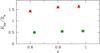 |
Fig. 8 Ratio between half of the aperture of the slit and effective radius of the galaxies as a function of the mean stellar mass density and z. The colour code is the same as in Fig. 6. |
In Fig. 8, the points indicate the portion of galaxy covered by the slit in Re unit for the high-Σ and low-Σ sub-populations, as a function of redshift. Almost all of the light from high-Σ MPGs is included in the slit, thus the D4000n provides constraints on the age of the whole galaxy, similarly to the SED fitting. For low-Σ MPGs, the slit samples the inner 0.5 Re. Given the known presence of metallicity gradients in passive galaxies both in local Universe and at intermediate redshift, this implies that at any redshift i) we cannot directly compare the D4000n of high- and low-Σ MPGs; and ii) for low-Σ MPGs, we cannot directly compare the results from SED fitting with those derived from the spectral features as we did for high-Σ MPGs. Although a direct comparison at fixed redshift is not straightforward, we highlight that the region which is sampled by the slit is approximately constant over our redshift range (see Fig. 8) and this assures us that the evolutionary trends of D4000n are not affected by aperture effects.
Taking advantage of the spatially resolved information on stellar population properties provided by ATLAS3D survey (Cappellari et al. 2011) for a sample of 260 local elliptical galaxies (ETGs), we quantified that for low-Σ local massive ETGs the metallicity in the central (r<0.5Re, ZRe/2) region is ~20% greater than the metallicity within Re (see Appendix C). At the same time, we found that there is no significant trend with radius of the timescale of the star formation or age4. Taking this into consideration, we derived D4000n,SED applying the correction we derived from local Universe to the mean values of Z (we note that Gallazzi et al. (2014) do not find any evolution in the metallicities of massive quiescent galaxies since z~0.8). Results are shown as open green squares in the right panel of Fig. 7. As for high-Σ MPGs, they are in good agreement with the D4000n values measured on real spectra. To qualitatively show the effect of slit aperture, we report in the figure also the values of D4000n,SED not corrected for the aperture bias. There is clear disagreement between these values and the mean values measured from real spectra.
Summarizing, both the evolution of the number density and of the stellar population ages of low-Σ MPGs strongly support a picture in which younger low-Σ MPGs continuously appear at lower redshift. These results indicate that the increase both in number and in mean size of the population of MPGs is due to the continuous addition of larger and younger quiescent galaxies over cosmic time.
We stress that the comparison between D4000n and D4000n,SED in Fig. 7 is meaningful only between the mean values of the distributions and not for any single galaxy. Conventionally SED modelling uses a coarse grid of Z/τ, that cannot accurately reproduce the more realistic smooth distributions of metallicity and timescale of star formation of real galaxies. Nonetheless, although the single values of stellar population parameters could be biased, the mean values are more representative of the truth as suggested by the consistency between D4000n and D4000n,SED in Fig. 7. Although the consistency between spectroscopic and photometric data confirms the robustness of our conclusions, we are conscious of the issues related to the Age and Z derived from SED fitting. For this reason we derived the stellar population ages also using only the D4000n measurements. To do this, we followed the standard approach of assuming some fiducial values for Z and τ from local studies (e.g. Fagioli et al. 2016; Zahid et al. 2016). We caution that in this analysis we are interested just in relative values of stellar population ages, i.e. in the ΔAge from z = 1.0 and z = 0.5, and not in the absolute values. This relaxed requirement alleviates the issue related to the unknown value of τ. In fact, Fig. A.1 shows that at fixed metallicity and in the range of ages we are interested in, the curves with different τ are almost parallel (see the figure for models in which Z = Z⊙ and τ = 0.3, 0.4, and 0.6 Gyr respectively). This fact implies that the ΔAge does not depend much on τ but mostly on Z. Using our analysis on ATLAS3D survey, we fixed Z = 0.85Z⊙ for low-Σ MPGs (see Appendix C, [Z/H] Re/ 2). In Fig. A.1, the evolution of D4000n as a function of age for this Z value is plotted. We obtained the curve interpolating the models with Z = Z⊙ and Z = 0.4 Z⊙. The value of D4000n for low-Σ MPGs at z = 1.0 and z = 0.5 (i.e. 1.74 and 1.84, see Fig. 7) is also shown. We observe that the corresponding ΔAge is <1 Gyr, i.e. the evolution of the stellar population ages is slower than that expected in case of passive evolution (ΔAge = 2 Gyr), as we found in Fig. 7. We notice that this conclusion is still valid also for solar and super-solar metallicity. Following the same scheme, we repeat the analysis for high-Σ MPGs. In this case we fixed Z = 0.7 Z⊙ (see Appendix C, [Z/H] Re). As before, in Fig. A.1 we indicate the evolution of D4000n for this Z value and also plot the value of D4000n at z = 1.0 and z = 0.5 (i.e. 1.67 and 1.80, see Fig. 7). The figure shows that ΔAge is ~1.7 Gyr, which is consistent within the errors with the ΔAge expected in case of a passive evolution, in agreement with our conclusions of Fig. 7. For completeness, we also plot the evolution of D4000n as a function of age for Z = 0.5Z⊙, that is for the Z value we obtained from the best fit of the SED.
Evidence for older ages of the densest galaxies has been found by many authors both in the local Universe and at high-z (e.g. Shankar & Bernardi 2009; Saracco et al. 2009; Valentinuzzi et al. 2010; Williams et al. 2010; Saracco et al. 2011; Poggianti et al. 2013a; Carollo et al. 2013; Fagioli et al. 2016). However most of these works investigated a larger stellar mass range, not focusing their analysis on the massive end.
In the same mass range, using UV colour to date stellar population ages of passive compact massive ellipticals, Carollo et al. (2013) found that they are consistent with passive evolution, in agreement with our results. Using a set of Lick absorption indices, Onodera et al. (2015) investigated stellar population properties for a sample of massive quiescent galaxies (UVJ colour selected) at ⟨ z ⟩ = 1.6. They found a mean age of 1.1 Gyr. As stated by the authors, this value is in excellent agreement with the age of local counterparts, if high-z massive quiescent galaxies evolve passively. We verified that more than 80% of their sample is composed of massive passive galaxies with Σ>2000 M⊙ pc-2, thus we can reasonably compare their results with ours. If we assume passive evolution between z = 1.6 and z = 0.95, the mean age of their massive quiescent galaxies rises to 3.1 Gyr. This is in fair agreement with the mean age of high-Σ MPGs we find at z = 0.95 (3.7 ± 0.2 Gyr) (see also Whitaker et al. 2013).
Different conclusions were reached by F16. Using stacked spectra, the authors constrained the stellar population ages for dense and less dense passive galaxies in the zCOSMOS sample from z = 0.8 to z = 0.2. They found that the age of dense massive quiescent galaxies increases less than would be expected from passive evolution alone. Moreover, they found no correlation between the age of stellar population and the dimension of the source. The present analysis differs from the F16 analysis in a number of ways: the selection of passive galaxies (no emission lines plus no MIPS in F16 vs. NUVrK colour in our work); the selection of the dense sub-population (cut at fixed Re or along the SMR vs. cut at fixed Σ); and the procedure adopted to constrain the stellar population age. Unfortunately, we cannot exactly reproduce their analysis with our data set. In Appendix B, we checked how our results change if we adopt the same criteria used by F16 to select dense and less dense galaxies. We found that the mean age of dense MPGs is consistent with passive evolution and that less dense MPGs are younger than dense MPGs, independently of the criteria used to divide the sub-populations. However, as stated above, we stress that the previous checks rely on a sample of MPGs selected in a different way and adopt different techniques to constrain the stellar population age. In fact, we cannot repeat the same analysis with our data set, so we cannot fully account for the effect of these two factors on the results.
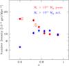 |
Fig. 9 Evolution of the number density of MPGs (filled red circles) and of star forming massive galaxies (MSFGs, blue filled stars). Open circles show the expected growth in the abundance of MPGs below z<0.8, assuming that this is fully due to the observed decline of MSFGs. Solid and open circles have been shifted for visualisation purposes. |
6. Where do new large MPGs come from?
The evidence that the new MPGs are systematically younger than high-Σ MPGs contrasts with the hypothesis that all massive galaxies are assembled mostly through dry mergers (e.g. Hopkins et al. 2009; Cappellari et al. 2012). In fact, dry mergers should dilute any trend between stellar population age and time of appearance by mixing up the stellar population of pre-existing systems. In fact, more recently new pieces of evidence have come to light supporting a scenario in which PGs are mostly the final evolutionary stage of star-forming galaxies (SFGs) that progressively halt their star formation until they become quiescent (e.g. Lilly & Carollo 2016; Driver et al. 2013; Huertas-Company et al. 2015, 2016). In fact, at any z and at fixed stellar mass, star-forming galaxies are larger than passive ones (e.g. van der Wel et al. 2014). Thus, if passive galaxies are just the quenched counterpart of star-forming galaxies, we should expect a correlation between the stellar population age of PGs and their mean stellar mass density in the direction of younger age for less dense systems. This is exactly what we have shown in Fig. 7. In this case, however, further evidence is expected: the number of PGs that appear at any time, has to be similar to the number of SFGs that disappear. To test this simple hypothesis, in Fig. 9 we compare the number density of the whole population of MPGs, with the number density of massive star-forming galaxies (MSFGs). We considered all non passive massive galaxies to be MSFGs. The figure shows that the number densities of the two populations start to deviate at z<0.8, that is when the Universe becomes efficient at producing low-Σ MPGs. In particular, the number density of MSFGs is almost flat at z> 0.8 and then drops by a factor of approximately 2 at lower z. The declining trend does not depend on the selection criterion used to identify MSFGs. Haines et al. (2017) found the same trend studying the number density of  1011 M⊙ VIPERS galaxies with D4000n<1.55. Starting from the very simple assumption that all the MSFGs that disappear at z<0.8, must necessarily migrate in the population of MPGs, we derived the number density of MPGs expected at z<0.8 by considering their density at z = 0.8 and the observed decrement of MSFGs at z<0.8. Open red symbols report the results. In fact, they are in excellent agreement with the observed number density of MPGs. In this basic test we did not take into account the fact that some star-forming galaxies with ℳ<1011 M⊙ can enter into our sample at a later time. Nevertheless, the comparison shown in Fig. 9 shows that, to first order, the migration of MSFGs to MPGs fully accounts for the increase in the number density of MPGs with cosmic time. In particular the ⟨ Re ⟩ of MSFGs at z~0.8 is ~5.7 kpc, in agreement with the value ⟨ Re ⟩ = 6.3 ± 3 kpc of low- and intermediate-Σ MPGs at ⟨ z ⟩ = 0.5. If a portion of low-Σ MPGs assembled its stellar mass inside-out, that is starting from a compact passive core, we should add the number of these size-evolved MPGs to the open circles in Fig. 9, since the “progenitor” compact core is not included in the population of MSFGs. In fact, including other channels for MPG production in the model would overestimate the number density of the population. We can therefore exclude the possibility that the inside-out accretion scenario is the main channel for the build up of the MPG population. This evidence confirms in an independent way the results we found in Figs. 6 and 7 and that we summarise in the cartoon of Fig. 10. In the ~2.5 Gyr of time from z = 1.0 to z = 0.5, the number density of high-Σ MPGs does not evolve, and the ages of their stellar populations are consistent with a passive evolution. In the same time interval, the number density of low-Σ MPGs increases by a factor of four. This increase is fully consistent with the decrement we observe in the number density of MSFGs. If the new low-Σ MPGs are the direct descendants of MSFGs, we should expect to find that the new low-Σ MPGs would have to be younger than low-Σ MPGs and high-Σ MPGs already in place at higher redshift, as we found in Fig. 7.
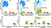 |
Fig. 10 Schematic view of our results and findings. In the lower panels we plot the evolution of number density for low- and high-Σ MPGs (large green and small red dark spheroids, respectively). From z = 1.0 to z = 0.5 the number density of high-Σ MPGs does not increase, while over the same time period, the number of low-Σ MPGs increases by a factor 4. These new low-Σ MPGs are plausibly the direct descendants of MSFGs (blue spirals) that progressively halt their star formation until they become passive (see upper panels). In fact, we found that the observed increase in the number density of MPGs is totally accounted for by the observed decrease in the number density of MSFGs. |
7. Summary and conclusions
We used the VIPERS data set to investigate how the population of massive passive galaxies (MPGs) has been built up over cosmic time.
We looked at the evolution of both the number density and the mean age of the stellar population of MPGs as a function of redshift, and of the mean surface stellar mass density. From the VIPERS data set, we selected a sample of ~2000 MPGs over the redshift range 0.5z1.0. We divided this sample into three sub-populations according to their value of Σ: high-Σ MPGs, intermediate-Σ MPGs, and low-Σ MPGs.
We studied the evolution of the number density for the three sub-populations of MPGs and found that it depends on Σ: the lower Σ the faster the evolution (see Fig. 6). In particular, we found that the number of dense galaxies per unit volume does not increase from z = 1.0 to z = 0.5. Instead, over the same time interval, the number density of less dense MPGs increases by a factor 4. This different evolution changes the composition of the population of MPGs with time. At z>0.8, high-, intermediate- and low-Σ MPGs contribute approximately equally to the population. At z<0.8, the number density of low-Σ MPGs progressively increases and this sub-population starts to dominate over the other two classes.
We then investigated the evolution of the stellar population ages as a function of Σ (see Fig. 7). We constrained the ages using both photometry, that is fitting the spectral energy distribution, and spectroscopy, through the D4000n index (Balogh et al. 1999). These two independent estimates are in agreement and show that:
-
The evolution of the age of high-Σ MPGs is fully consistent with apassive ageing of their stellar population.
-
The evolution of the age of low-Σ MPGs is slower than would be expected in the case of passive evolution, i.e. new low-Σ MPGs are younger than existing ones.
-
At any redshift, dense MPGs are older than less dense MPGs.
Both the evolution of the number density and of the age of the stellar population of high-Σ MPGs are consistent with passive evolution for this sub-population. On the other hand, the results we found for low-Σ MPGs show that their number density continuously increases with decreasing redshift, that is new low-Σ galaxies join the population of MPGs as time goes by. The study of stellar population age shows that these new galaxies are systematically younger than the low-Σ MPGs already in place.
These results indicate that the increase both in number density and in typical radial size observed for the population of MPGs is mostly due to the addition of less dense and younger galaxies at later times. Taking the results for low- and high-Σ MPGs together we found that the population of MPGs was built by the continuous addition of less dense MPGs: on top of passively evolving dense MPGs already in place at z = 1.0, new, larger and younger quiescent galaxies continuously join the population of MPGs at later times.
We find evidence that these new MPGs are the direct descendants of massive star-forming galaxies (MSFGs) that quenched their star formation. In fact, in Fig. 9 we show that the observed increase in the number density of MPGs is totally accounted for by the decrease in the number density of MSFGs. This not only provides constraints on the origin of MPGs, but also rules out inside-out accretion as the main channel for their build up, confirming in an independent way our conclusions based on the evolution of number density and stellar population age.
We caution that this value refers to the whole galaxy, not just to the central region known to have Z>ZSun (e.g. Gallazzi et al. 2005). This value is in agreement with the mean metallicity within Re of local massive ETGs (0.7 Z⊙, see Appendix C).
The population of passive galaxies and elliptical galaxies are not coincident (see e.g. Tamburri et al. 2014; Moresco et al. 2013). However, at first order, the two populations share the same properties.
Acknowledgments
We acknowledge the crucial contribution of the ESO staff for the management of service observations. In particular, we are deeply grateful to M. Hilker for his constant help and support of this programme. Italian participation to VIPERS has been funded by INAF through PRIN 2008, 2010, and 2014 programmes. L.G., A.J.H., and B.R.G. acknowledge support from the European Research Council through grant No. 291521. O.L.F. acknowledges support from the European Research Council through grant No. 268107. T.M. and S.A. acknowledge financial support from the ANR Spin(e) through the french grant ANR-13-BS05-0005. A.P., K.M., and J.K. have been supported by the National Science Centre (grants UMO-2012/07/B/ST9/04425 and UMO-2013/09/D/ST9/04030). W.J.P. is also grateful for support from the UK Science and Technology Facilities Council through the grant ST/I001204/1. E.B., F.M. and L.M. acknowledge the support from grants ASI-INAF I/023/12/0 and PRIN MIUR 2010-2011. L.M. also acknowledges financial support from PRIN INAF 2012. S.D.L.T. acknowledges the support of the OCEVU Labex (ANR-11-LABX-0060) and the A*MIDEX project (ANR-11-IDEX-0001-02) funded by the “Investissements d’Avenir” French government programme managed by the ANR. and the Programme National Galaxies et Cosmologie (PNCG). Research conducted within the scope of the HECOLS International Associated Laboratory, supported in part by the Polish NCN grant DEC-2013/08/M/ST9/00664.
References
- Arnouts, S., Le Floc’h, E.,Chevallard, J., et al. 2013, A&A, 558, A67 [NASA ADS] [CrossRef] [EDP Sciences] [Google Scholar]
- Balogh, M. L., Morris, S. L., Yee, H. K. C., Carlberg, R. G., & Ellingson, E. 1999, ApJ, 527, 54 [NASA ADS] [CrossRef] [Google Scholar]
- Belli, S., Newman, A. B., & Ellis, R. S. 2014, ApJ, 783, 117 [NASA ADS] [CrossRef] [Google Scholar]
- Bertin, E., & Arnouts, S. 1996, A&AS, 117, 393 [NASA ADS] [CrossRef] [EDP Sciences] [Google Scholar]
- Bezanson, R., van Dokkum, P. G., Tal, T., et al. 2009, ApJ, 697, 1290 [NASA ADS] [CrossRef] [Google Scholar]
- Bolzonella, M., Miralles, J.-M., & Pelló, R. 2000, A&A, 363, 476 [NASA ADS] [Google Scholar]
- Brammer, G. B., Whitaker, K. E., van Dokkum, P. G., et al. 2011, ApJ, 739, 24 [NASA ADS] [CrossRef] [Google Scholar]
- Bruzual, G., & Charlot, S. 2003, MNRAS, 344, 1000 [NASA ADS] [CrossRef] [Google Scholar]
- Calzetti, D., Armus, L., Bohlin, R. C., et al. 2000, ApJ, 533, 682 [NASA ADS] [CrossRef] [Google Scholar]
- Cappellari, M., Emsellem, E., Krajnović, D., et al. 2011, MNRAS, 413, 813 [NASA ADS] [CrossRef] [Google Scholar]
- Cappellari, M., McDermid, R. M., Alatalo, K., et al. 2012, Nature, 484, 485 [NASA ADS] [CrossRef] [Google Scholar]
- Cappellari, M., Scott, N., Alatalo, K., et al. 2013, MNRAS, 432, 1709 [NASA ADS] [CrossRef] [Google Scholar]
- Carollo, C. M., Bschorr, T. J., Renzini, A., et al. 2013, ApJ, 773, 112 [NASA ADS] [CrossRef] [Google Scholar]
- Cassata, P., Giavalisco, M., Guo, Y., et al. 2010, ApJ, 714, L79 [NASA ADS] [CrossRef] [Google Scholar]
- Cassata, P., Giavalisco, M., Guo, Y., et al. 2011, ApJ, 743, 96 [NASA ADS] [CrossRef] [Google Scholar]
- Cassata, P., Giavalisco, M., Williams, C. C., et al. 2013, ApJ, 775, 106 [NASA ADS] [CrossRef] [Google Scholar]
- Chabrier, G. 2003, PASP, 115, 763 [NASA ADS] [CrossRef] [Google Scholar]
- Cimatti, A., Daddi, E., Renzini, A., et al. 2004, Nature, 430, 184 [NASA ADS] [CrossRef] [PubMed] [Google Scholar]
- Cimatti, A., Cassata, P., Pozzetti, L., et al. 2008, A&A, 482, 21 [NASA ADS] [CrossRef] [EDP Sciences] [Google Scholar]
- Daddi, E., Renzini, A., Pirzkal, N., et al. 2005, ApJ, 626, 680 [NASA ADS] [CrossRef] [Google Scholar]
- Damjanov, I., Abraham, R. G., Glazebrook, K., et al. 2011, ApJ, 739, L44 [NASA ADS] [CrossRef] [Google Scholar]
- Damjanov, I., Hwang, H. S., Geller, M. J., & Chilingarian, I. 2014, ApJ, 793, 39 [NASA ADS] [CrossRef] [Google Scholar]
- Damjanov, I., Geller, M. J., Zahid, H. J., & Hwang, H. S. 2015, ApJ, 806, 158 [NASA ADS] [CrossRef] [Google Scholar]
- Davidzon, I., Bolzonella, M., Coupon, J., et al. 2013, A&A, 558, A23 [NASA ADS] [CrossRef] [EDP Sciences] [Google Scholar]
- Davidzon, I., Cucciati, O., Bolzonella, M., et al. 2016, A&A, 586, A23 [NASA ADS] [CrossRef] [EDP Sciences] [Google Scholar]
- De Lucia, G., & Blaizot, J. 2007, MNRAS, 375, 2 [NASA ADS] [CrossRef] [Google Scholar]
- Dekel, A., Birnboim, Y., Engel, G., et al. 2009, Nature, 457, 451 [NASA ADS] [CrossRef] [PubMed] [Google Scholar]
- Driver, S. P., Robotham, A. S. G., Bland-Hawthorn, J., et al. 2013, MNRAS, 430, 2622 [NASA ADS] [CrossRef] [Google Scholar]
- Fagioli, M., Carollo, C. M., Renzini, A., et al. 2016, ApJ, 831, 173 [NASA ADS] [CrossRef] [Google Scholar]
- Franx, M., & van Dokkum, P. G. 1996, in New Light on Galaxy Evolution, eds. R. Bender, & R. L. Davies, IAU Symp., 171, 233 [Google Scholar]
- Fritz, A., Scodeggio, M., Ilbert, O., et al. 2014, A&A, 563, A92 [NASA ADS] [CrossRef] [EDP Sciences] [Google Scholar]
- Gallazzi, A., Charlot, S., Brinchmann, J., White, S. D. M., & Tremonti, C. A. 2005, MNRAS, 362, 41 [NASA ADS] [CrossRef] [Google Scholar]
- Gallazzi, A., Bell, E. F., Zibetti, S., Brinchmann, J., & Kelson, D. D. 2014, ApJ, 788, 72 [NASA ADS] [CrossRef] [Google Scholar]
- Gargiulo, A., Saracco, P., Longhetti, M., La Barbera, F., & Tamburri, S. 2012, MNRAS, 425, 2698 [NASA ADS] [CrossRef] [Google Scholar]
- Gargiulo, A., Saracco, P., Tamburri, S., Lonoce, I., & Ciocca, F. 2016, A&A, 592, A132 [NASA ADS] [CrossRef] [EDP Sciences] [Google Scholar]
- Garilli, B., Le Fèvre, O., Guzzo, L., et al. 2008, A&A, 486, 683 [NASA ADS] [CrossRef] [EDP Sciences] [Google Scholar]
- Garilli, B., Guzzo, L., Scodeggio, M., et al. 2014, A&A, 562, A23 [NASA ADS] [CrossRef] [EDP Sciences] [Google Scholar]
- Guo, Y., Giavalisco, M., Cassata, P., et al. 2011, ApJ, 735, 18 [NASA ADS] [CrossRef] [Google Scholar]
- Guzzo, L., Scodeggio, M., Garilli, B., et al. 2014, A&A, 566, A108 [NASA ADS] [CrossRef] [EDP Sciences] [Google Scholar]
- Haines, C. P., Iovino, A., Krywult, J., et al. 2017, A&A, 605, A4 [NASA ADS] [CrossRef] [EDP Sciences] [Google Scholar]
- Hilz, M., Naab, T., & Ostriker, J. P. 2013, MNRAS, 429, 2924 [NASA ADS] [CrossRef] [Google Scholar]
- Hopkins, P. F., Cox, T. J., & Hernquist, L. 2008, ApJ, 689, 17 [NASA ADS] [CrossRef] [Google Scholar]
- Hopkins, P. F., Bundy, K., Murray, N., et al. 2009, MNRAS, 398, 898 [NASA ADS] [CrossRef] [Google Scholar]
- Huertas-Company, M., Pérez-González, P. G., Mei, S., et al. 2015, ApJ, 809, 95 [NASA ADS] [CrossRef] [Google Scholar]
- Huertas-Company, M., Bernardi, M., Pérez-González, P. G., et al. 2016, MNRAS, 462, 4495 [NASA ADS] [CrossRef] [Google Scholar]
- Ilbert, O., Salvato, M., Le Floc’h, E., et al. 2010, ApJ, 709, 644 [NASA ADS] [CrossRef] [Google Scholar]
- Jarvis, M. J., Bonfield, D. G., Bruce, V. A., et al. 2013, MNRAS, 428, 1281 [NASA ADS] [CrossRef] [Google Scholar]
- Kauffmann, G., Heckman, T. M., White, S. D. M., et al. 2003, MNRAS, 341, 33 [NASA ADS] [CrossRef] [Google Scholar]
- Kereš, D., Katz, N., Weinberg, D. H., & Davé, R. 2005, MNRAS, 363, 2 [NASA ADS] [CrossRef] [Google Scholar]
- Krywult, J., Tasca, L. A. M., Pollo, A., et al. 2017, A&A, 598, A120 [NASA ADS] [CrossRef] [EDP Sciences] [Google Scholar]
- La Barbera, F., & de Carvalho, R. R. 2009, ApJ, 699, L76 [NASA ADS] [CrossRef] [Google Scholar]
- Le Fèvre, O., Vettolani, G., Garilli, B., et al. 2005, A&A, 439, 845 [NASA ADS] [CrossRef] [EDP Sciences] [Google Scholar]
- Lilly, S. J., & Carollo, C. M. 2016, ApJ, 833, 1 [NASA ADS] [CrossRef] [Google Scholar]
- Lilly, S. J., Le Fèvre, O., Renzini, A., et al. 2007, ApJS, 172, 70 [NASA ADS] [CrossRef] [Google Scholar]
- Longhetti, M., Saracco, P., Severgnini, P., et al. 2007, MNRAS, 374, 614 [NASA ADS] [CrossRef] [Google Scholar]
- McDermid, R. M., Alatalo, K., Blitz, L., et al. 2015, MNRAS, 448, 3484 [NASA ADS] [CrossRef] [Google Scholar]
- Moresco, M., Pozzetti, L., Cimatti, A., et al. 2013, A&A, 558, A61 [NASA ADS] [CrossRef] [EDP Sciences] [Google Scholar]
- Moutard, T., Arnouts, S., Ilbert, O., et al. 2016a, A&A, 590, A102 [NASA ADS] [CrossRef] [EDP Sciences] [Google Scholar]
- Moutard, T., Arnouts, S., Ilbert, O., et al. 2016b, A&A, 590, A103 [NASA ADS] [CrossRef] [EDP Sciences] [Google Scholar]
- Naab, T., Johansson, P. H., Ostriker, J. P., & Efstathiou, G. 2007, ApJ, 658, 710 [NASA ADS] [CrossRef] [Google Scholar]
- Naab, T., Johansson, P. H., & Ostriker, J. P. 2009, ApJ, 699, L178 [NASA ADS] [CrossRef] [Google Scholar]
- Onodera, M., Carollo, C. M., Renzini, A., et al. 2015, ApJ, 808, 161 [NASA ADS] [CrossRef] [Google Scholar]
- Peng, C. Y., Ho, L. C., Impey, C. D., & Rix, H. 2002, AJ, 124, 266 [NASA ADS] [CrossRef] [Google Scholar]
- Poggianti, B. M., Calvi, R., Bindoni, D., et al. 2013a, ApJ, 762, 77 [NASA ADS] [CrossRef] [Google Scholar]
- Poggianti, B. M., Moretti, A., Calvi, R., et al. 2013b, ApJ, 777, 125 [NASA ADS] [CrossRef] [Google Scholar]
- Pozzetti, L., Bolzonella, M., Zucca, E., et al. 2010, A&A, 523, A13 [NASA ADS] [CrossRef] [EDP Sciences] [Google Scholar]
- Prevot, M. L., Lequeux, J., Prevot, L., Maurice, E., & Rocca-Volmerange, B. 1984, A&A, 132, 389 [NASA ADS] [Google Scholar]
- Qu, Y., Helly, J. C., Bower, R. G., et al. 2017, MNRAS, 464, 1659 [NASA ADS] [CrossRef] [Google Scholar]
- Saglia, R. P., Fabricius, M., Bender, R., et al. 2010, A&A, 509, A61 [NASA ADS] [CrossRef] [EDP Sciences] [Google Scholar]
- Salpeter, E. E. 1955, ApJ, 121, 161 [Google Scholar]
- Saracco, P., Longhetti, M., & Andreon, S. 2009, MNRAS, 392, 718 [NASA ADS] [CrossRef] [Google Scholar]
- Saracco, P., Longhetti, M., & Gargiulo, A. 2010, MNRAS, L115 [Google Scholar]
- Saracco, P., Longhetti, M., & Gargiulo, A. 2011, MNRAS, 412, 2707 [NASA ADS] [CrossRef] [Google Scholar]
- Scodeggio, M., Guzzo, L., Garilli, B., et al. 2017, A&A, in press, DOI: 10.1051/0004-6361/201630114 [Google Scholar]
- Shankar, F., & Bernardi, M. 2009, MNRAS, 396, L76 [NASA ADS] [CrossRef] [Google Scholar]
- Shen, S., Mo, H. J., White, S. D. M., et al. 2003, MNRAS, 343, 978 [NASA ADS] [CrossRef] [Google Scholar]
- Siudek, M., Małek, K., Scodeggio, M., et al. 2017, A&A, 597, A107 [NASA ADS] [CrossRef] [EDP Sciences] [Google Scholar]
- Spolaor, M., Kobayashi, C., Forbes, D. A., Couch, W. J., & Hau, G. K. T. 2010, MNRAS, 408, 272 [NASA ADS] [CrossRef] [Google Scholar]
- Tamburri, S., Saracco, P., Longhetti, M., et al. 2014, A&A, 570, A102 [NASA ADS] [CrossRef] [EDP Sciences] [Google Scholar]
- Trujillo, I., Feulner, G., Goranova, Y., et al. 2006, MNRAS, 373, L36 [NASA ADS] [CrossRef] [Google Scholar]
- Valentinuzzi, T., Fritz, J., Poggianti, B. M., et al. 2010, ApJ, 712, 226 [NASA ADS] [CrossRef] [Google Scholar]
- van der Wel, A., Holden, B. P., Zirm, A. W., et al. 2008, ApJ, 688, 48 [NASA ADS] [CrossRef] [Google Scholar]
- van der Wel, A., Franx, M., van Dokkum, P. G., et al. 2014, ApJ, 788, 28 [NASA ADS] [CrossRef] [Google Scholar]
- van Dokkum, P. G., Franx, M., Kriek, M., et al. 2008, ApJ, 677, L5 [NASA ADS] [CrossRef] [Google Scholar]
- Whitaker, K. E., van Dokkum, P. G., Brammer, G., et al. 2013, ApJ, 770, L39 [NASA ADS] [CrossRef] [Google Scholar]
- Williams, R. J., Quadri, R. F., Franx, M., van Dokkum, P., & Labbé, I. 2009, ApJ, 691, 1879 [NASA ADS] [CrossRef] [Google Scholar]
- Williams, R. J., Quadri, R. F., Franx, M., et al. 2010, ApJ, 713, 738 [NASA ADS] [CrossRef] [Google Scholar]
- Zahid, H. J., Baeza Hochmuth, N., Geller, M. J., et al. 2016, ApJ, 831, 146 [NASA ADS] [CrossRef] [Google Scholar]
Appendix A: The dependence of D4000n on metallicity, timescale of star formation, resolution and IMF.
In Fig. A.1 we report D4000n for different BC03 models in order to show the dependence of this quantity on metallicity, timescale of star formation, spectral resolution and IMF. We plot lines that track the evolution of D4000n with stellar population age for BC03 low resolution (lr) models with the same star formation timescale (τ = 0.4 Gyr) and Z = 0.2 Z⊙, Z = 0.5 Z⊙, Z = 0.7 Z⊙, Z = 0.85 Z⊙, Z = Z⊙, and Z = 2.5 Z⊙. We also show the evolution of D4000n for models with solar metallicity and τ = 0.3 Gyr and τ = 0.6 Gyr, along with D4000n for two models with the same τ and metallicity but different resolution. In particular, starting from a high resolution BC03 model with τ = 0.4 Gyr and Z = 0.2 Z⊙ we downgrade it to 20 Å and to 17 Å , the typical resolution of VIPERS spectra. Finally, we plot the evolution of the D4000n index for a model with τ = 0.4 Gyr, Z = 2.5 Z⊙ and the Salpeter IMF (Salpeter 1955).
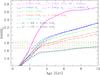 |
Fig. A.1 D4000n index as a function of the age for BC03 low resolution models with exponentially declining star formation history, the Chabier IMF (when not otherwise specified), and different τ and Z. Solid magenta, solid blue, solid green, solid red, red-dashed and solid cyan lines correspond to models with τ = 0.4 Gyr and Z = 2.5 Z⊙, Z⊙, 0.85 Z⊙, 0.7 Z⊙, 0.5 Z⊙ and 0.2 Z⊙. Dashed and dot-dashed blue lines indicate models with Z = Z⊙ and τ = 0.3 Gyr and 0.6 Gyr, respectively. Dotted and dashed black lines indicate models with Z = 0.2 Z⊙, τ = 0.4 Gyr and resolution 20 Å and 17 Å respectively. Dot-dashed magenta line indicates the evolution of D4000n index for models with Z = 2.5 Z⊙, τ = 0.4 Gyr and the Salpeter IMF (Salpeter 1955). Dashed horizontal green and red lines indicate the value of D4000n at z = 1.0 and at z = 0.5 for low- and high-Σ MPGs, respectively. |
Appendix B: Comparison with the analysis by Fagioli et al.
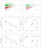 |
Fig. B.1 Upper panels: selection criteria of dense and less dense MPGs in this work and in F16 work reported in the size mass plane, in two redshift bins (0.5 |
In this section we repeat the analysis shown in Sect. 5 assuming the same definition for dense and less dense passive galaxies adopted by Fagioli et al. (2016). As stated in Sect. 5, Fagioli et al. adopted two criteria to select dense and non dense galaxies: i) cuts at constant Re (i.e. Re<4.5 kpc for dense galaxies and Re> 7.5 kpc for less dense galaxies); and ii) cuts parallel to the SMR. In this second case, the authors fixed the slope to 0.63 and, in any redshift bin, varied the zero-point such to split the sample in three sub-populations which account for the 35:30:35% of the total number of galaxies in the redshift bin under consideration. In the upper panels of Fig. B.1 the selection criteria are shown for the two extreme redshift bins (0.5z<0.7 in the left panel and 0.9z1.0 in the right panel).
In the middle left panel of Fig. B.1 we plot the evolution of ageSED for MPGs with Re<4.5 kpc and with Re>7.5 kpc. In the figure, we also track the evolution for the pure aging of the stellar populations from z = 0.95 to z = 0.6. The figure shows that the ageSED of MPGs with Re<4.5 kpc are consistent with a passive evolution, and that at any z, less dense galaxies are younger. The middle right panel shows the evolution of the mean D4000n for the two sub-populations. D4000n values expected from the results of the SED fitting (D4000n,SED, see Sect. 5 for more details on the procedure) are indicated in the right panel. The agreement between D4000n and D4000n,SED is overall good and confirms the results we found in Sect. 5 for our sample of dense and less dense MPGs.
Lower panels in Fig. B.1 show the same of the upper panels but for galaxies selected with cut parallel to the SMR. Even in this case, the general conclusions do not change.
Appendix C: Impact of the finite dimension of the slit on the estimate of D4000n for low-Σ MPGs
In Sect. 5 we mentioned that the 1′′ slit of VIPERS spectra just samples the central (r<0.5Re) regions of low-Σ MPGs and up to 1.5Re for high-Σ MPGs. Given the presence of metallicity gradients in passive galaxies, this peculiarity can invalidate the direct comparison of D4000n for MPGs with different Σ and also the comparison between the stellar ages derived from the fit of the SED (considering the whole galaxy) and the D4000n values for low-Σ MPGs. In this section we want to quantify if and how much the stellar population properties vary with the radius in passive galaxies, in order to interpret our results at the light of these constraints.
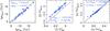 |
Fig. C.1 Left panel: stellar population age within 0.5 Re vs. the stellar population age within Re for local ETGs with dynamical mass log MJAM>10.9 and Σ<1000 M⊙ pc-2 (green points). Solid line is the 1:1 correlation. Mean value of ages at Re and at 0.5 Re are reported in the panel. Central and right panels: as left panel but for stellar metallicity and α enhancement, respectively. |
We address this topic using the spatially resolved information on stellar population properties provided by ATLAS3D survey (Cappellari et al. 2011) for a sample of local ETGs. In particular we refer to the estimates of age, metallicity and alpha enhancement [α/Fe] within Re and whitin 0.5 Re presented in McDermid et al. (2015). Stellar masses were not provided by the ATLAS3D team; for this reason we refer to the dynamical masses MJAM derived as specified in Table 1 in Cappellari et al. (2013) (M/LJAM × L, the median dark matter fraction is just 13%, see Cappellari et al. 2013). From the same table we took the Re values and derived the mean stellar mass density as MJAM/(2π ). From the whole sample of 260 ETGs we selected the massive (log MJAM>10.9) and less dense galaxies Σ (<1000 M⊙ pc-2). We relaxed the mass cut somewhat with respect to the one used in the paper to have a higher statistic (considering that here we are using total mass). In Fig. C.1 we report the age, metallicity and [α/Fe] measured within 0.5 Re versus their estimates within Re for local massive less dense ETGs. Figure C.1 shows that the central regions of local ETGs have approximately the same age and [α/Fe] of the external regions (AgeRe/Age0.5 Re≃1.05, [α/FeRe]/[α/ Fe0.5 Re]≃1.0) but are more metal rich (Z0.5 Re/ZRe≃1.2, for similar results see also Spolaor et al. 2010).
All Tables
Best-fit values (α, β) of the size mass relation log Re = αlog (ℳ/1011) + β of VIPERS MPGs.
Total number of massive quiescent galaxies and of the high-Σ sample, intermediate-Σ sample, and low-Σ sample in the four redshift bins 0.5z<0.7, 0.7<z0.8, 0.8<z0.9, 0.9<z1.0.
All Figures
|
Fig. 1 Ratio between the effective radius in r band (Re,r) and the effective radius in i band (Re,i) as a function of Re,i for MPGs in three bins of redshift as indicated in the top left corner of each plot. In the three panels, the solid blue lines are the best fit relations derived with a sigma-clipping algorithm. Dashed blue lines set the 1σ deviation. The typical dimension of half of the PSF-FWHM of both i-band and r-band images is indicated in the top right corner of each plot with also the number of objects. Open red circles are galaxies at >3σ from this fit. |
| In the text | |
|
Fig. 2 Fraction of MPGs with available Re in the W1 field (magenta filled points), in the W4 field (blue filled points) as a function of z. At z<0.8, MPGs with Re derived from i-band images are included. Red filled points indicate the completeness for the W1+W4 field. |
| In the text | |
|
Fig. 3 Size-mass relation of passive VIPERS galaxies (grey open + red open points) in the two extreme redshift bins of our analysis (0.5 |
| In the text | |
|
Fig. 4 Distribution of the effective radius for MPGs in our lowest (blue histogram) and highest (red histogram) redshift bins. The solid lines indicate the median values of the two distributions. The probability p that the two distributions are extracted from the same parent sample are reported in the label. |
| In the text | |
|
Fig. 5 Number densities for massive passive galaxies with Σ≥2000 M⊙ pc-2 (right panel, dark red symbols), 1000≤Σ<2000 M⊙ pc-2 (central panel, orange symbols), and Σ<1000 M⊙ pc-2 (left panel, green symbols), for the W1 field (filled circles) and W4 one (open circles). Number densities for the W4 field are shifted in redshift to better visualize them. The error bars correspond to 1σ. |
| In the text | |
|
Fig. 6 Number density of MPGs with different mean stellar mass density in VIPERS field as a function of the redshift. Dark red triangles refer to high-Σ MPGs, orange circles refer to intermediate-Σ MPGs, and green squares to low-Σ MPGs. Black circles show the number density for the total sample of MPGs. Number densities for the three sub-populations are shifted in redshift to better visualize them. The error bars correspond to 1σ. We fitted the data with a power law and solid lines are the best-fit relations. |
| In the text | |
|
Fig. 7 Left panel: mean stellar population ages of MPGs as derived from the SED fitting as a function of redshift and mean stellar mass density for high- and low-Σ MPGs (filled points). The colour and symbols code is the same as in Fig. 6. Error bars indicate the error on the mean. Points refer to the redshift bins 0.5 |
| In the text | |
|
Fig. 8 Ratio between half of the aperture of the slit and effective radius of the galaxies as a function of the mean stellar mass density and z. The colour code is the same as in Fig. 6. |
| In the text | |
|
Fig. 9 Evolution of the number density of MPGs (filled red circles) and of star forming massive galaxies (MSFGs, blue filled stars). Open circles show the expected growth in the abundance of MPGs below z<0.8, assuming that this is fully due to the observed decline of MSFGs. Solid and open circles have been shifted for visualisation purposes. |
| In the text | |
|
Fig. 10 Schematic view of our results and findings. In the lower panels we plot the evolution of number density for low- and high-Σ MPGs (large green and small red dark spheroids, respectively). From z = 1.0 to z = 0.5 the number density of high-Σ MPGs does not increase, while over the same time period, the number of low-Σ MPGs increases by a factor 4. These new low-Σ MPGs are plausibly the direct descendants of MSFGs (blue spirals) that progressively halt their star formation until they become passive (see upper panels). In fact, we found that the observed increase in the number density of MPGs is totally accounted for by the observed decrease in the number density of MSFGs. |
| In the text | |
|
Fig. A.1 D4000n index as a function of the age for BC03 low resolution models with exponentially declining star formation history, the Chabier IMF (when not otherwise specified), and different τ and Z. Solid magenta, solid blue, solid green, solid red, red-dashed and solid cyan lines correspond to models with τ = 0.4 Gyr and Z = 2.5 Z⊙, Z⊙, 0.85 Z⊙, 0.7 Z⊙, 0.5 Z⊙ and 0.2 Z⊙. Dashed and dot-dashed blue lines indicate models with Z = Z⊙ and τ = 0.3 Gyr and 0.6 Gyr, respectively. Dotted and dashed black lines indicate models with Z = 0.2 Z⊙, τ = 0.4 Gyr and resolution 20 Å and 17 Å respectively. Dot-dashed magenta line indicates the evolution of D4000n index for models with Z = 2.5 Z⊙, τ = 0.4 Gyr and the Salpeter IMF (Salpeter 1955). Dashed horizontal green and red lines indicate the value of D4000n at z = 1.0 and at z = 0.5 for low- and high-Σ MPGs, respectively. |
| In the text | |
|
Fig. B.1 Upper panels: selection criteria of dense and less dense MPGs in this work and in F16 work reported in the size mass plane, in two redshift bins (0.5 |
| In the text | |
|
Fig. C.1 Left panel: stellar population age within 0.5 Re vs. the stellar population age within Re for local ETGs with dynamical mass log MJAM>10.9 and Σ<1000 M⊙ pc-2 (green points). Solid line is the 1:1 correlation. Mean value of ages at Re and at 0.5 Re are reported in the panel. Central and right panels: as left panel but for stellar metallicity and α enhancement, respectively. |
| In the text | |
Current usage metrics show cumulative count of Article Views (full-text article views including HTML views, PDF and ePub downloads, according to the available data) and Abstracts Views on Vision4Press platform.
Data correspond to usage on the plateform after 2015. The current usage metrics is available 48-96 hours after online publication and is updated daily on week days.
Initial download of the metrics may take a while.