| Issue |
A&A
Volume 605, September 2017
|
|
|---|---|---|
| Article Number | A69 | |
| Number of page(s) | 18 | |
| Section | Interstellar and circumstellar matter | |
| DOI | https://doi.org/10.1051/0004-6361/201630308 | |
| Published online | 11 September 2017 | |
Far-infrared HD emission as a measure of protoplanetary disk mass
1 Leiden Observatory, Leiden University, Niels Bohrweg 2, 2333 CA Leiden, The Netherlands
e-mail: trapman@strw.leidenuniv.nl
2 Max-Planck-institute für extraterrestrische Physic, Giessenbachstraße, 85748 Garching, Germany
Received: 21 December 2016
Accepted: 17 May 2017
Context. Protoplanetary disks around young stars are the sites of planet formation. While the dust mass can be estimated using standard methods, determining the gas mass – and thus the amount of material available to form giant planets – has proven to be very difficult. Hydrogen deuteride (HD) is a promising alternative to the commonly used gas mass tracer, carbon monoxide. However, the potential of HD has not yet been investigated with models incorporating both HD and CO isotopologue-specific chemistry, and its sensitivity to uncertainties in disk parameters has not yet been quantified.
Aims. We examine the robustness of HD as tracer of the disk gas mass, specifically the effect of gas mass on HD far-infrared emission and its sensitivity to the vertical structure. Also, we seek to provide requirements for future far-infrared missions such as SPICA.
Methods. Deuterium chemistry reactions relevant for HD were implemented in the thermochemical code DALI and more than 160 disk models were run for a range of disk masses and vertical structures.
Results. The HD J = 1–0 line intensity depends directly on the gas mass through a sublinear power law relation with a slope of ~0.8. Assuming no prior knowledge about the vertical structure of a disk and using only the HD 1–0 flux, gas masses can be estimated to within a factor of two for low mass disks (Mdisk ≤ 10-3M⊙). For more massive disks, this uncertainty increases to more than an order of magnitude. Adding the HD 2–1 line or independent information about the vertical structure can reduce this uncertainty to a factor of ~ 3 for all disk masses. For TW Hya, using the radial and vertical structure from the literature, the observations constrain the gas mass to 6 × 10⁻³M⊙ ≤ Mdisk ≤ 9 × 10⁻³M⊙. Future observations require a 5σ sensitivity of 1.8 × 10⁻²⁰ W m-2 (2.5 × 10⁻²⁰ W m-2) and a spectral resolving power R ≥ 300 (1000) to detect HD 1–0 (HD 2–1) for all disk masses above 10-5M⊙ with a line-to-continuum ratio ≥ 0.01.
Conclusions. These results show that HD can be used as an independent gas mass tracer with a relatively low uncertainty and should be considered an important science goal for future far-infrared missions.
Key words: protoplanetary disks / astrochemistry
© ESO, 2017
1. Introduction
One of the key properties for understanding the evolutionary path of disks and the formation of planets is the disk gas mass (e.g. Armitage 2015). Determining gas masses is not an easy task. The main component of the gas, molecular hydrogen (H2), is difficult to observe. As a symmetric rotor, H2 has no electric dipole moment, limiting its rotational lines to quadrupole transitions (ΔJ = 2). The J = 2 level lies at 549.2 K, therefore to produce any appreciable H2 emission gas temperatures have to be at least 100 K (Thi et al. 2001; Carmona et al. 2011), which is much higher than the temperature of the bulk of the gas in the disk. In addition, these lines lie in the mid- and near-infrared (IR) where the continuum is bright, which further hampers the observations due to the high continuum optical depth and low line-to-continuum ratios. Even if detected, the H2 emission does not trace the bulk of the mass (e.g. Pascucci et al. 2013). This means that indirect tracers of the gas mass have to be used.
Historically, most of the disk mass estimates have been based on observations of the (sub-)millimeter (mm) emission of the dust grains (e.g. Beckwith et al. 1990; Dutrey et al. 1996; Mannings & Sargent 1997; Williams et al. 2005). In order to relate the observed flux to the mass of the emitting material, a mass opacity κν and a temperature Tdust have to be assumed (cf. Hildebrand 1983). To obtain the total (gas+dust) mass, the estimate of the dust mass has to be scaled up by the gas-to-dust mass ratio. Usually the interstellar medium (ISM) value of 100 is assumed, but it is unclear whether this is applicable to protoplanetary disks.
The gaseous component of the disk can be traced using carbon monoxide (CO), the second most abundant molecule in the disk, which is readily detected towards many protoplanetary disks (e.g. Dutrey et al. 1996; Thi et al. 2001; Dent et al. 2005; Panić et al. 2008; Williams & Best 2014). To derive a gas mass from CO observations, a relation has to be found between the amount of CO in the disk and the amount of H2. In the simplest case, where most of the available carbon is contained in gas-phase CO, the fractional abundance of CO is n(CO) /n(H2) ~ 2 × 10⁻⁴ in line with observations of warm dense clouds (e.g. Lacy et al. 1994).
In protoplanetary disks there are two processes that decrease the CO abundance below its maximum value (van Zadelhoff et al. 2001). In the upper layer of the disk, CO is being destroyed through photodissociation by ultraviolet (UV) photons. In the midplane, where temperatures are below ~ 20 K, CO freezes out onto the dust grains. As a result of these non-linear processes, thermochemical models have to be used to relate CO observations to the total gas mass. These processes are well understood and they are implemented in current thermochemical models. However, studies that include these effects have found that overall gas phase carbon must still be additionally depleted by a factor 10–100. This leads to low CO emission even for massive disks (e.g. Bruderer et al. 2012; Favre et al. 2013; Du et al. 2015; Kama et al. 2016b; Bergin et al. 2016).
Several processes have been proposed to explain the underabundance of gas-phase carbon in regions where freeze-out is not important. A possible explanation could be grain growth, where carbon has been locked up in large icy bodies that no longer participate in the gas-phase chemistry (see e.g. Bergin et al. 2010, 2016; Du et al. 2015; Kama et al. 2016b). Another cause could be the conversion of CO into more complex species. This process can happen in the gas phase through reactions between CO and He+, which extracts atomic carbon that can then be used to construct more complex molecules. These molecules have higher freeze-out temperatures than CO and freeze out onto the cold grains, thus lowering the apparent carbon abundance (Aikawa et al. 1997; Favre et al. 2013; Bergin et al. 2014). Similarly, ice chemistry can play an important role in converting CO into more complex organics, such as CH3OH or turning it into CO2 or CH4 ice (see e.g. Fig. 3c in Eistrup et al. 2016).
Owing to its high abundance, 12CO becomes optically thick at the disk surface, meaning it does not trace the bulk of the mass. Instead, less abundant CO isotopologues such as 13CO, C18O, and C17O have to be used, which remain optically thin throughout the disk (van Zadelhoff et al. 2001; Dartois et al. 2003). Visser et al. (2009) and Miotello et al. (2014) showed that the C18O/C16O ratio is reduced beyond the 18O/16O isotope ratio in disks owing to isotope-selective photodissociation. Not taking this effect into account can change the estimated mass using C18O up to one order of magnitude (Miotello et al. 2014).
Using the Herschel Space Observatory, hydrogen deuteride (HD) has been detected towards TW Hya, DM Tau, and GM Aur (Bergin et al. 2013; McClure et al. 2016). HD has been suggested as an alternative tracer of the disk gas mass. Because of their chemical similarities, the distribution of HD is expected to closely follow that of H2. HD has a small dipole moment, so dipole transitions (ΔJ = 1) are allowed. The difference between the energy needed to excite the first rotational level of HD (E/kB ≃ 128.5 K) and the energy needed to excite the second rotational level of H2 (E/kB ≃ 549.2 K) means that at a temperature of T ~ 20 K the expected emission of HD is much larger than that of H2.
The energetically lowest transition of HD, J = 1–0, emits at 112 μm (Müller et al. 2005). This places the transition in a wavelength range where the dust continuum is bright, the atmospheric opacity is high, and the production of low-noise detectors is expensive. All these reasons combined make detecting HD a challenge. Even with Herschel, deep integrations were required to observe HD in disks. After the end of the Herschel mission, there are currently no far-IR observatories capable of detecting HD in disks. However, this may change with the advent of future far-IR missions such as the proposed SPICA mission (Nakagawa et al. 2014) and with the HIRMES instrument on SOFIA.
In this work, a simple HD chemistry is incorporated into the thermochemical code Dust and Lines (DALI; Bruderer et al. 2012; Bruderer 2013). In Sect. 2 a description of the code is given, including the deuterium chemistry that was implemented. A description of the models run is also given here. In Sect. 3 the dependence of the HD far-infrared emission on the disk gas mass is examined. In addition, the effect of other disk properties such as the vertical structure and the dust distribution on the HD emission is investigated. Furthermore, the results are examined in the light of possible future far-IR missions such as SPICA. The effect of prior knowledge of the disk vertical structure on the uncertainty of the HD based mass estimates is discussed in Sect. 4. Additionally, the models are compared to the current observations. Of particular interest is the protoplanetary disk of TW Hya (59.54 ± 1.45 pc, Astraatmadja & Bailer-Jones 2016), where the gas mass estimated with HD is more than one order of magnitude higher than the gas mass estimated with C18O (Favre et al. 2013). Various studies have shown that the TW Hya disk seems genuinely depleted in volatile carbon and oxygen (e.g. Bergin et al. 2010, 2013, 2016; Hogerheijde et al. 2011; Favre et al. 2013; Du et al. 2015; Kama et al. 2016b). Recently, new observations of the CO isotopologues have become available (see e.g. Schwarz et al. 2016). Therefore, the case of TW Hya is revisited using a combined HD and CO isotopologue analysis. The conclusions can be found in Sect. 5.
2. Model
The thermochemical code Dust and Lines (DALI) was used to calculate the line fluxes for the disk models (Bruderer et al. 2012; Bruderer 2013). This 2D physical-chemical code calculates the thermal and chemical structure self-consistently for a given physical disk model. In addition to the density structure of the disk, a stellar spectrum has to be provided to determine the UV radiation field inside the disk. The computation proceeds through three steps. First the dust temperature structure and internal radiation field (from UV- to mm-wavelengths) are determined by solving the continuum radiative transfer using a 2D Monte Carlo method. Next, the abundances of the molecular and atomic species at each point of the disk are obtained from the solution of the time-dependent chemistry. The atomic and molecular excitations are then computed with a non-LTE calculation. Given the excitation levels, the gas temperature is determined by balancing the heating and cooling processes. Because both the chemistry and excitations depend on temperature, the problem is solved iteratively until a self-consistent solution is found. Lastly, the model is ray-traced to construct spectral image cubes and line profiles. A more detailed description of the code can be found in Appendix A of Bruderer et al. (2012).
2.1. Density structure
The density structure used in the code follows the simple parametric model proposed by Andrews et al. (2011). This model is based on the assumption that the disk structure is determined by viscous accretion, where the viscosity goes as ν ∝ Rγ (Lynden-Bell & Pringle 1974; Hartmann et al. 1998). The resulting surface density is given by ![\begin{equation} \Sigma_{\rm gas}(R) = \Sigma_{\rm c} \left( \frac{R}{R_{\rm c}}\right)^{\gamma} \exp \left[ -\left(\frac{R}{R_{\rm c}}\right)^{2-\gamma}\right]\cdot \label{eq: surface density} \end{equation}](/articles/aa/full_html/2017/09/aa30308-16/aa30308-16-eq37.png) (1)Here Σc is the surface density at the characteristic radius Rc.
(1)Here Σc is the surface density at the characteristic radius Rc.
The vertical structure is given by a Gaussian density distribution, as motivated by hydrostatic equilibrium (Kenyon & Hartmann 1987) ![\begin{eqnarray} n(R,z) &=& \frac{1}{\sqrt{2 \pi}}\frac{1}{H} \exp \left[ -\frac{1}{2}\left(\frac{z}{H}\right)^2\right] \label{eq: vertical density}\\ &=& \frac{1}{\sqrt{2 \pi}}\frac{1}{Rh} \exp \left[ -\frac{1}{2}\left(\frac{z/R}{h}\right)^2\right], \end{eqnarray}](/articles/aa/full_html/2017/09/aa30308-16/aa30308-16-eq40.png) where H = Rh is the physical height of the disk and the scale height angle h is parametrized by
where H = Rh is the physical height of the disk and the scale height angle h is parametrized by 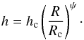 (4)Here hc is the scale height at Rc and ψ is known as the flaring angle. Equation (4)is a representation of a physical disk, where the vertical structure is set by balancing gravity and the vertical pressure gradient at each point in the disk.
2.2. Dust settling
In order to include dust settling into the model, the dust grains are split into two populations:
-
Small grains (0.005–1 μm) are included with a (mass) fractional abundance 1−flarge. These are located throughout the vertical extent of the disk.
-
Large grains (1–103μm) are included with a fractional abundance flarge. They are limited to a vertical region with scale height χh; χ< 1, simulating the effect of dust settling.
 |
Fig. 1 Gas and dust density structure assumed in DALI. |
In contrast to earlier versions of DALI, the current version of DALI only couples the gas surface density profile to the density profile of the small grains. The resulting disk structure is summarized in Fig. 1.
A standard ISM dust composition is assumed for the dust opacities following Weingartner & Draine (2001), in line with Bruderer (2013; see e.g. his Fig. 2). The mass opacities for absorption at 112 μm and 56 μm for both dust grain populations are given in Table 1.
Dust mass opacities.
2.3. Chemical network
For the models in this work the list of chemical species adopted in Miotello et al. (2014) was extended to include HD, D, HD+, and D+ as separate species. By adding the element D to H, He, 12C, 13C, N, 16O, 17O, 18O, Mg, Si, S, and Fe, the total number of species was increased to 280. The reaction types included are H2 and HD formation on dust, freeze-out, thermal and non-thermal desorption, hydrogenation of simple species on ices, gas-phase reactions, photodissociation, X-ray and cosmic-ray induced reactions, PAH and small grain charge exchange and hydrogenation, and reactions with H (vibrationally excited H2). The details of the implementation of these reactions are described in Appendix A.3.1 of Bruderer et al. (2012).
To properly simulate HD integrated line fluxes, simple deuterium chemistry was added to the chemical network. The only D-bearing species considered for the chemical calculation are D, D+, HD, and HD+. Accordingly, the important reactions regulating their abundances were included with rate coefficients from Roberts & Millar (2000) and Walmsley et al. (2004). Photodissociation of HD was included following Glover & Jappsen (2007). The photodissociation rate for a radiation field with a flat spectrum is given by Eq. (51), in Glover & Jappsen (2007), 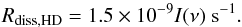 (5)Here I(ν) is the mean intensity of the radiation field. The prefactor has units such that the photodissociation rate has units [s-1].
HD self-shielding was also included in the model using the shielding function of H2 but is slightly shifted in wavelength. Finally HD formation onto grains and ion-exchange reactions with metals and PAHs were included with the same rate coefficients as that assumed for the analogue reactions with H instead of D. The reactions involving D-bearing species added in the chemical network are presented in Table D.1 in Appendix D.
2.4. Grid of models
As a basis for the models, we used the physical structure of the TW Hya disk from the Kama et al. (2016b) model. A combination of spatially and spectrally resolved and unresolved line fluxes, together with observations of the spectral energy distribution (SED), was used to constrain the parameters of their model, which can be found in Table 2. Kama et al. (2016b) have found a strongly flared vertical structure for TW Hya. Also, their model has a radially steeper temperature profile and smaller outer radius than the models of Cleeves et al. (2015).
In total, over a 160 models were run via DALI. The employed chemical network is the expanded version of that used by Miotello et al. (2014), where simple deuterium chemistry has been considered (see Sect. 2.3). The input total disk masses are Mdisk = [2.6 × 10⁻⁵, 2.6 × 10⁻⁴, 7.7 × 10⁻⁴, 2.6 × 10⁻³, 7.7 × 10⁻³, 2.3 × 10⁻², 7.7 × 10⁻², 2.6 × 10⁻¹]M⊙. For each mass, 20 models with different vertical structures were run, i.e. hc ∈ [0.05,0.1,0.2,0.3] ,ψ ∈ [0.1,0.2,0.3,0.4,0.5] (cf. Eq. (4)). The other parameters were kept fixed to the values assumed by Kama et al. (2016b) (Table 2). For the overall carbon and oxygen abundances, typical ISM values of [C]/[H]ISM = 1.35×10⁻⁴, [O]/[H]ISM = 2.88 × 10⁻⁴ were used (Bruderer et al. 2012).
 |
Fig. 2 Left panel: integrated line flux (calculated at 140 pc) of the HD 1–0 transition as a function of disk mass. The points show the median flux of the models in that mass bin. The blue shaded region shows fluxes between the 16th and 84th percentiles in the same mass bin. The blue line shows the fit of Eq. (6)using the values from Table 3. Right panel: integrated line flux (calculated at 140 pc) of the HD 2–1 transition as a function of disk mass. |
The stellar spectrum for TW Hya from Cleeves et al. (2015) was used as the central source of radiation. It closely resembles a 4000 K blackbody with a 10 000 K blackbody component to represent the observed UV excess (following the prescription in Kama et al. 2016a, see also Fig. 3 and Table 3 in Kama et al. 2016b).
DALI parameters of the physical model.
The time-dependent chemistry was run for 1 Myr, which is less than the expected age for TW Hya, but the HD emission is not sensitive to the chemical age.
The overall deuterium abundance [D]/[H] of the gas in the disk has a direct impact on the HD fluxes. Prodanović et al. (2010) have used observations of the atomic D and H lines in the diffuse ISM to find ([D] / [H] )ISM ≥ (2.0 ± 0.1) × 10-5 for the local ISM (i.e. within ~ 1−2 kpc of the Sun). The uncertainties due to the error on the assumed [D]/[H] found by Prodanović et al. (2010) are much smaller than the spread in HD fluxes due to the disk structure. For older star forming regions, such as Orion, the deuterium abundance is lower because a fraction of the deuterium has been burned up in the cores of stars (Wright et al. 1999; Howat et al. 2002).
3. Results
3.1. HD flux versus disk gas mass
The first step in investigating the viability of HD as a tracer of the disk gas mass is examining the behaviour of its emission under variations of the gas mass. This is presented in Fig. 2, where the integrated HD 1–0 and 2–1 line fluxes are plotted as functions of disk mass. In the left panel of Fig. 2 the blue dots shows the median HD 1–0 flux for each disk mass, while the coloured region presents fluxes between the 16th and 84th percentiles in each mass bin. The HD 1–0 line flux increases with mass, following a linear dependence in log-log space for the low mass disks (Mdisk ≤ 10-3M⊙).
Towards the high mass regime, the relation flattens. There are two reasons for this change in behaviour. For disk masses above 0.001 M⊙ the HD 1–0 line emission starts to become optically thick, which means that the HD emission no longer traces the full gas reservoir. In addition, high mass disks have larger densities, which decreases the gas temperature in the disk. Miotello et al. (2016) found a similar decrease in line luminosity for 13CO and C18O in high mass disks, which they attributed to optical depth for 13CO and increased freeze-out for C18O.
The right panel of Fig. 2 shows that the flux-mass relation for the HD 2–1 line is flatter compared to HD 1–0. This is likely due to increased temperature dependence of the HD 2–1 line compared to the HD 1–0 line. The increased temperature dependence is reflected in the increased sensitivity of HD 2–1 to the vertical structure of the disk, as indicated by the large flux variations in each mass bin.
The behaviour of the flux-mass relation can be expressed with an analytical relation, such as 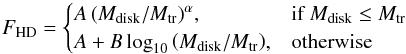 (6)where Mtr is defined as the mass where the flux-mass relation starts to flatten.
This model was fitted to the median fluxes of both HD lines. The resulting coefficients can be found in Table 3. The power-law slopes for both HD lines are sublinear. This is likely a result from the fact that the HD emission is produced by warm gas only.
Fit coefficients of the HD flux-mass relation.
3.2. HD emitting layers
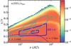 |
Fig. 3 HD abundance structure for a disk model with Mdisk = 2.3 × 10⁻²M⊙, ψ = 0.3 and hc = 0.1. Colour indicates the number density of HD with respect to the total gas density. The coloured lines correspond the HD 1–0 (blue) and HD 2–1 (light blue), respectively. Solid contours indicate where 25% and 75% of the emission originates from. The dashed (dash-dotted) lines show the τ = 1 surface for the line and continuum opacity, respectively. |
The 2D abundance of HD in a typical model is presented in Fig. 3. This distribution is the outcome of the deuterium chemical calculation discussed in Sect. 2.3. We point out that n(HD) /ngas = 2 × 10⁻⁵ throughout most of the disk, indicating that all of the available deuterium is locked up in HD. The exceptions to this rule are in the upper layer of the disk, where HD is photodissociated, and in an intermediate layer, where HD abundance is decreased by a factor of ~2. This layer is due to a combination of chemical processes. This layer is very thin and only covers a very small fraction of the HD emission area shown in Fig. 3. Therefore the depletion in this layer has no relevant effect on the HD flux.
The solid blue lines in Fig. 3 denote where 25% and 75% of the HD 1–0 emission is produced. This region is elevated above the midplane (0.1 ≤ z/r ≤ 0.25), indicating that most of the HD 1–0 emission is produced by warm gas with an average temperature of 30−70 K (cf. Fig. A.2). The emitting region extends radially from rin ≈ 9 AU up to rout ≈ 70 AU for Mdisk = 2.3 × 10⁻²M⊙. The inner and outer radii vary slightly in vertical structure (cf. Fig. B.1). Figure B.2 shows that when the disk gas mass is increased the emitting region shifts outward, from (rin,rout) ≈ (1 AU,40 AU) for Mdisk = 2.3 × 10⁻⁵M⊙ to (rin,rout) ≈ (10 AU,100 AU) for Mdisk = 2.3 × 10⁻¹M⊙. This is a result of the optically thick HD zone extending to larger radii as the gas mass increases.
The τ = 1 surfaces for the line and continuum optical depth are shown in dashed and dash-dotted lines, respectively. They show that continuum optical depth has no effect on the line emission. This is likely because most of the dust mass is in large grains, which are settled to the midplane in contrast with the models by Bergin et al. (2014). The dashed line shows that for this model with Mdisk = 2.3 × 10⁻²M⊙, the HD emission starts to become optically thick, which is in line with the flattening of the slope seen in Fig. 2.
For the HD 2–1 emission, shown in light blue in Fig. 3, the emission originates even higher up in the disk, where gas temperatures are in the range of 70−100 K (cf. Fig. A.2). The contour for the line optical depth shows that the HD 2–1 emission starts to become optically thick in the inner part of the disk for Mdisk = 2.3 × 10⁻²M⊙.
3.3. Influence of the vertical structure
 |
Fig. 4 Integrated HD 1–0 (top) and HD 2–1 (bottom) line fluxes as functions of flaring angle ψ for different scale heights hc. The fluxes are normalized with respect to median flux of the models with the same disk mass (cf. Fig. 2). |
The strength of the HD emission depends on the amount of material and the temperature of the material. In protoplanetary disks the temperature structure is set by the vertical structure of the disk (Chiang & Goldreich 1997). The effect of the vertical structure on the HD 1–0 and 2–1 fluxes is presented in Fig. 4. This figure shows the HD fluxes as functions of the flaring angle ψ for different scale heights hc (colours). This was carried out for three different mass bins (2.3 × 10⁻⁵M⊙, 2.3 × 10⁻³M⊙, and 2.3 × 10⁻¹M⊙). The fluxes in each mass bin are normalized with respect to the median flux in the same bin (cf. blue dots in Fig. 2).
The normalized HD 1–0 integrated line fluxes are presented in top panels of Fig. 4. It shows that the HD 1–0 flux increases with increasing ψ. The relation is roughly linear with a slope that is independent of hc and Mdisk.
The spacing between the different hc lines indicate that the HD 1–0 flux also increases systematically with hc. The shape of the flux-hc relation depends only weakly on ψ. The shape depends strongly on disk mass with the influence of hc on the flux increasing as a function of disk mass.
For HD 2–1, presented in the bottom panels of Fig. 4, the dependencies of the flux on hc and ψ are stronger than those found for HD 1–0. The bulk of the HD 2–1 emission is produced by gas at temperatures of 70−100 K (cf. Fig. A.2). This gas is located higher up in the disk. As the optically thin HD 2–1 emission depends on both the temperature and density, the location of the HD 2–1 emitting material varies strongly with vertical structure, as can be seen in Fig. B.1. This is in contrast to the HD 1–0 emitting material, which stays at roughly the same location, independent of the vertical structure.
Figure 4 shows that the maximum variation in flux due to different vertical structures increases with disk mass, from 0.75 × the median flux for Mdisk ~ 10-5M⊙ up to 1.9 × the median flux for Mdisk ~ 10-1M⊙. For the HD 2–1 integrated line flux, shown in the bottom panel of Fig. 4, the maximum variation in flux is both larger than for HD 1–0 and less dependent on disk mass. The maximum variation of the flux is 1.9 × the median flux for Mdisk ~ 10-5M⊙, increasing to 2.8 × the median flux for Mdisk ~ 10-1M⊙. As mentioned in Sect. 3.2, the regions where the HD lines are optically thick have larger outer radii as the gas mass is increased. On the one hand, this pushes the HD emitting regions upwards to parts of the disk that are more sensitive to the vertical structure. On the other hand, the increased size of the optically thick HD zone means that, for massive disks, a larger mass fraction of HD will be much warmer as the vertical structure changes. The uncertainty in derived gas masses from HD due to vertical structure is further quantified in Sect. 4.1.
In the above models, the vertical structure is parametrized according to Eq. (4). Another approach would be to calculate the vertical structure using hydrostatic equilibrium from the computed gas temperature structure. The effect of this approach on the HD fluxes is examined in Appendix C and is found to be within the flux variations shown in Fig. 4.
3.4. Influence of the large grains
For the models discussed in Sect. 2.4 only three parameters (Mdisk, ψ and hc) were varied. However, several other parameters may also affect the HD flux. Their role is investigated here. In particular, the large dust grains in the disk can affect the HD flux, both by affecting heating and by changing the optical depth of the dust at the wavelengths where HD emits. Two dust parameters are examined here: the mass fraction of the large grains flarge and the dust settling parameter of the large grains χ (cf. Sect. 2.2). In both cases, the mass and vertical structure of the disk were fixed to the values from Kama et al. (2016b). The resulting HD 1−0 fluxes, normalized to the median flux of the Mdisk = 2.3 × 10⁻²M⊙ mass bin, are shown in Fig. 5.
 |
Fig. 5 Integrated line flux of HD 1–0 as a function of dust parameters for Mdisk = 2.3×10⁻²M⊙. Models with different flarge and χ are shown in orange and green, respectively. The fluxes are normalized to the median flux of the Mdisk = 2.3 × 10⁻²M⊙ mass bin. The triangular marker denotes the value of the parameter (flarge or χ) in the fiducial model of the TW Hya disk (Kama et al. 2016b; cf. Table 2). |
Figure 5 shows that the HD 1–0 flux increases with dust settling (i.e. when the large grains are more settled towards the midplane). This can be understood by the fact the dust optical depth at a fixed height in the disk increases when the large grain population (cf. Sect. 2.2) is less settled. This is especially the case in the model for TW Hya, where most of the dust mass is in these grains.
A similarly large effect is found when the mass fraction of the large grains is changed. When flarge decreases, the amount of small grains increases significantly, which increases the opacity at 112 μm.
Comparing these results with those from the previous section, it is clear that both the large grains and the vertical structure have similar effects on the HD 1–0 line flux. However, both χ and flarge are constrained by the SED (e.g. D’Alessio et al. 2001; Chiang et al. 2001), so their values cannot be chosen arbitrarily.
3.5. Influence of the gas-to-dust ratio
Deriving accurate gas-to-dust mass ratios has been one of the motivations for measuring the gas mass directly (e.g. Ansdell et al. 2016; Miotello et al. 2017). However, the gas-to-dust ratio could also affect the HD emission directly, for example by changing the coupling between the dust and gas. If the effect is strong it may prevent accurate measurements of the gas-to-dust ratio using gas masses derived from HD emission. For fixed gas mass of Mgas = 2.3 × 10⁻²M⊙, Fig. 6 presents the HD 1–0 fluxes as a function of increasing gas-to-dust ratio (and therefore decreasing dust mass). The fluxes are normalized with respect to the median flux of the Mdisk = 2.3 × 10⁻²M⊙ mass bin.
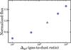 |
Fig. 6 Integrated line flux of HD 1–0 as a function of the gas-to-dust mass ratio for fixed gas mass (Mgas = 2.3 × 10⁻²M⊙). The fluxes are normalized to the median flux of the Mdisk = 2.3 × 10⁻²M⊙ mass bin. The triangular marker denotes the value of Δgd in the fiducial model of the TW Hya disk (Kama et al. 2016b; cf. Table 2). |
The figure shows that the HD 1–0 flux increases systematically with Δgd. The primary reason for this is the decreased coupling between the gas and dust for higher gas-to-dust ratios. As the gas in the HD emitting region is less efficient in cooling than the dust, this leads to slightly higher gas temperatures. Additionally, the increased dust mass for the models with a lower Δgd enhances the dust opacities at the wavelengths where HD emits, which lowers the amount of observed line flux. However, inspection of the τdust = 1 surface at 112 μm shows that the increase in opacity is relatively small.
3.5.1. Determining gas-to-dust ratios using HD 1–0
Figure 6 shows that varying the gas-to-dust ratio by two orders of magnitude for a fixed gas mass only leads to a variation in the HD 1–0 line flux of ~ 1.5 × the median flux. In this analysis the dust mass is assumed to be a free parameter. However, in practice the dust mass of the observed disks is constrained, for example observing their millimeter-continuum fluxes. A comparison of HD 1–0 fluxes and millimeter continuum fluxes for models with different Δgd is shown in Fig. 7.
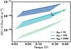 |
Fig. 7 HD 1–0 integrated fluxes and 870 μm continuum flux densities for the models described in Table 4. Colours indicate various gas-to-dust ratios, where the shaded region shows the flux variations from different vertical structures. For each Δgd, the coloured line shows models with (ψ,hc) = (0.3, 0.1). The crosses denote observations for TW Hya (black; Bergin et al. 2013; Andrews et al. 2012), DM Tau (purple; McClure et al. 2016; Andrews et al. 2013) and GM Aur (green; McClure et al. 2016; Andrews et al. 2013). Both the model fluxes and the observations were scaled to a distance of 140 pc. |
Here the HD emission is combined with the millimeter continuum emission of the dust to provide a method for estimating the gas-to-dust ratio from observations. For this purpose an additional set of 27 models was run, where the dust mass, gas-to-dust ratio, and vertical structure were varied (cf. Table 4). Figure 7 shows the HD 1−0 line flux, which traces the gas mass, plotted against the 870 μm continuum flux, which traces the dust mass. The lack of overlap between models with different gas-to-dust ratios indicates that combined observations of HD and the dust continuum can be used to determine Δgd. For the three disks for which HD 1–0 observations are available (i.e. TW Hya, DM Tau, and GM Aur) gas-to-dust ratios are found to be Δgd ~ 100, close to the ISM value. This would suggest that indeed the lower values found from similar measurements made using 13CO are due to an underabundance of volatile carbon (see Miotello et al. 2017, and references therein).
Disk parameters for the fixed dust mass models.
3.6. Line-to-continuum ratios
As mentioned in the introduction, observing lines in the far-infrared is inherently difficult because the emission of the dust in protoplanetary disks peaks at ~ 100 μm. Superimposed on this bright continuum are the intrinsically weak far-infrared lines. As a result, the line-to-continuum ratio (L/C) is a crucial ingredient for observing the HD levels.
The line-to-continuum ratio can be defined as  (7)Here Fline and Fcont are the continuum subtracted line flux and continuum flux, respectively. The approximation holds if the line is narrow, such that the integrated line flux can be approximated by the total flux in the centre-most frequency bin (Fpeak) times the bin width. In this case Fcont,bin is the continuum flux in the same bin.
Owing to the difficulties in characterizing the noise properties of infrared detectors and cosmic ray impacts on the detector and electronics, the current best achievable signal-to-noise ratio (S/N) for these detectors is ~300. In the most optimal case, these detectors are able to distinguish variations at the level of  of the source continuum flux. By requiring that the HD lines are detected at the 3σ level, the S/N = 300 translates into a detection limit of L/C≥3 × 0.0033 = 0.01, which cannot be improved by longer integration times.
The spectral resolving power R = λ/ Δλ of the instrument plays a crucial role in determining the L/C. As long as the line is unresolved, a higher R corresponds to a larger L/C, independent of the disk properties. This assumption is valid for the HD lines in protoplanetary disks, which are intrinsically narrow (FWHM~5 km s-1 in the outer disk). As explained in the introduction there is currently no facility capable of observing HD rotational transitions in disks. However, this work and previous studies (e.g. Bergin et al. 2013; McClure et al. 2016) have shown that HD is a unique tracer of the total gas mass. This means that the possibility of observing HD should be included in the consideration for instruments on future FIR observatories, such as the proposed SPICA mission. To be able to detect HD, the detection limit of L/C ≥ 0.01 places a constraint on the requirements of the spectral resolving power of these future FIR missions.
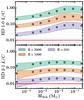 |
Fig. 8 Line-to-continuum ratios of HD as functions of Mdisk for different spectral resolving powers. The points show the median L/C of the models in the mass bin. The shaded region shows the L/Cs between the 16th and 84th percentile in each mass bin. The red line represents a 3σ detection limit of L/C= 0.01, which is equivalent to assuming a S/N on the continuum of 300. |
The top panel of Fig. 8 shows L/C for HD 1–0 as functions of disk mass for three different values of R. It is clear that the lower spectral resolving power mainly lowers the L/C. The current HD 1–0 detections with the Herschel PACS instrument are for R = 1000 at 112 μm. This figure demonstrates that future instruments, such as the SPICA SAFARI instrument (Roelfsema et al. 2014), need a resolving power of R ≥ 300 to detect HD 1–0 over the full mass range examined here, if a detection limit of L/C ≥ 0.01 (so S/N on the continuum of 300) is assumed. In the case of the HD 2–1 transition, shown in the bottom panel of Fig. 8, a spectral resolving power of R ≥ 1000 is required to detect HD 2–1 towards all disk masses above 10-5M⊙.
3.7. Sensitivities of future far-infrared missions
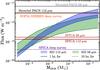 |
Fig. 9 HD 1–0 (blue) and 2–1 (green) model fluxes (calculated at 140 pc) as functions of disk gas mass (cf. Fig. 2). The horizontal lines represent the 5σ sensitivities for various instruments. The solid lines show the detection limit after 1 h of integration. The dashed lines show the 5σ sensitivity at 112 μm after 10 h of integration (labelled “deep survey”). |
In addition to good line-to-continuum ratios, future FIR missions also require good sensitivities to be able to detect the HD rotational lines in protoplanetary disks. In Fig. 9 the models presented in Fig. 2 are compared to the sensitivities of two FIR instruments: the proposed SPICA SAFARI instrument (Roelfsema et al. 2014) and the recently approved HIRMES instrument for SOFIA (E. Bergin, priv. comm.). The fluxes in the figure have been calculated for a distance of 140 pc, which is in line with typical distances to the closest star forming regions. The sensitivity of the Herschel PACS instrument is also shown here. The 5σ sensitivities after 1 hr of integration for SAFARI and Herschel PACS are shown in dark red and black, respectively. The purple and orange lines represent the 5σ sensitivities at 112 μm after 10 h of integration for the SAFARI and HIRMES instruments, respectively. Figure 9 shows that the proposed SPICA SAFARI instrument will be able to detect HD 1–0 in disks with gas masses down to 5 × 10⁻⁴M⊙ ≈ 0.5 Mjup. If the integration time is increased to 10 h the mass sensitivity goes down to 8 × 10⁻⁵M⊙ ≈ 0.08 Mjup.
4. Discussion
4.1. Determining the disk gas mass
In Sect. 3.1 the behaviour of the HD emission under variation of the disk gas mass was discussed. Figure 2 shows that it is possible to constrain the gas mass using the HD 1–0 flux. However, the variations in the flux due to the uncertainties on vertical structure translate into uncertainties in the determined gas mass. In this section these uncertainties are quantified and the impact of complementary observations on these uncertainties is investigated.
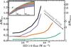 |
Fig. 10 Calculated mass uncertainties (cf. Eq. (8)) as functions of HD 1–0 flux. The left and right vertical axis are related via ΔMfactor = 10ΔMdex. The black line shows the result if the full set of models is used (cf. Table 2). The other three lines show results for weakly flared (purple), intermediately flared (orange) and strongly flared (light green) disks (see Table 5 for definitions for these subsets). The subsets are also shown in the top left panel, which shows a scaled version of Fig. 2. |
Figure 2 shows that models with different combinations of disk gas masses and vertical structures can produce the same HD 1–0 flux. The difference between the minimum and maximum disk mass, interpolated using the model fluxes shown in Fig. 2, can be used to quantify the uncertainty on the gas mass estimates using the flux (cf. the small panel in Fig. 10). Here the mass derivation uncertainty is defined as a factor of 10ΔM, where (8)Here Mmin(F), Mmax(F) are the minimum and maximum disk masses that can produce a HD 1–0 flux F, given the range of vertical structures examined.
The calculated mass uncertainties as functions of HD 1–0 flux are presented in Fig. 10. For the full set of models introduced in Sect. 2.4 (cf. Table 2), shown in black, ΔM increases with HD flux. The increase is steep, with ΔM=1 dex at a HD flux of ~ 5 × 10-19 W m-2, indicating that this flux corresponds to an estimated mass between 10-3M⊙ and 10-1M⊙.
This estimate relies only on the HD 1–0 flux without making any assumptions on the vertical structure of the disk. In practice, most disks also have been observed at other wavelengths and with other chemical tracers. These can be used to put constraints on the vertical structure of the disk. This would in turn lead to lower ΔM. If complementary observations can distinguish between weakly flared disks, intermediately flared disks and strongly flared disks (see Table 5 for the definitions), the uncertainties on the mass estimates can be significantly improved.
Definition of vertical structure classification.
The top left panel of Fig. 10 shows the three subsets with respect to the full set of models together with the mass uncertainties for each subset. For intermediately flared disks, shown in orange, ΔM is significantly lower compared to the full set. Here the maximum mass uncertainty is ~ 0.65 dex, meaning that the mass can be estimated within a factor of ~ 5.
For the strongly flared disks, shown in light green, the uncertainty is minimized and ΔM never becomes larger than 0.2 dex. As a result, masses for this subset can be estimated to within a factor of two.
The mass uncertainty for the weakly flared disks follows the uncertainty of the full sample, where ΔM is ~0.1 dex lower than for the full sample. For these ranges of hc and ψ the HD flux is very sensitive to the vertical structure, which results in variations in the flux comparable to those in the full set. However, a difference of 0.1 dex is still a factor of two improvement on the mass uncertainty.
4.2. HD 1–0 and HD 2–1 line fluxes
An interesting complementary observable is the HD 2–1 line emission. The main disk parameter determining the difference between the J = 1 and J = 2 level populations of HD is the gas temperature, which is largely set by the vertical structure. By combining observations of HD 2–1 and HD 1–0 this difference can be exploited to determine the disk mass with low uncertainty.
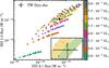 |
Fig. 11 HD 1–0 and HD 2–1 integrated fluxes (calculated at 140 pc) for the models described in Sect. 2.4. The different colours indicate different disk masses. The observations for TW Hya are shown in black (Bergin et al. 2013; Kama et al. 2016b; D. Fedele, priv. comm.). The bottom right corner shows the region around the observations, where the shaded regions link models that are within the same mass bin. |
As shown in Fig. 11, the different dependencies of HD 1–0 and HD 2–1 line fluxes on disk mass and vertical structure result in a clear mass segregation, independent of vertical structure. For disks with Mdisk ≥ 7.7 × 10⁻³M⊙ the mass bins start to overlap. As the bins differ by a factor of 3 in mass, the combination of two HD lines allow the gas mass to be determined to within a factor of ~3 provided that the observational uncertainties are small enough. To be able to determine the mass accurately across the whole mass range, the observational uncertainties have to decrease with increasing disk mass. This is not a too strict requirement as the observed line flux increases with disk mass, allowing for a more precise flux determination. The observations of HD 1–0 and HD 2–1 for TW Hya shown in Fig. 11 are discussed in Sect. 4.4.
4.3. Comparing models to observations
The HD 1–0 transition has been observed for three disks: TW Hya (Bergin et al. 2013), DM Tau, and GM Aur (McClure et al. 2016). These observations are shown in Fig. 12, which represents the high mass end of the left panel of Fig. 2. The observed flux for TW Hya was scaled to a distance of 140 pc, to allow for comparison with the same models.
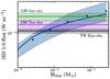 |
Fig. 12 Integrated line flux (calculated at 140 pc) of the HD 1–0 transition as a function of disk mass, representing the high mass end of the left panel of Fig. 2. The horizontal black solid line gives the observation of TW Hya, scaled to a distance of 140 pc, with the black shaded region representing the 1σ uncertainties (Bergin et al. 2013). The observations for DM Tau and GM Aur (McClure et al. 2016) are shown in purple and green, respectively. |
For DM Tau the lower limit on disk gas mass based on the HD 1–0 observation is Mdisk ≈ 4 × 10⁻³M⊙. This correspond to a high, strongly flared vertical structure. If instead the median vertical structure is assumed, the estimated gas mass becomes Mdisk ≈ 1.5 × 10⁻²M⊙. For GM Aur, a similar analysis gives a lower limit on the disk gas mass of Mdisk ≈ 1 × 10⁻²M⊙ for a high, strongly flared disk. Comparing the observed HD 1–0 flux to the medians, a gas mass of Mdisk ≈ 8 × 10⁻²M⊙ is found.
Both estimates based on the medians are in line with the results of McClure et al. (2016), who found gas masses of (1.0−4.5) × 10-2 and (2.5−19.5) × 10-2M⊙ for DM Tau and GM Aur by modelling both the HD flux and the continuum SED.
The observations for TW Hya shown in Fig. 12 are discussed in Sect. 4.4.
4.4. Case study: TW Hya
The protoplanetary disk of TW Hya (59.54 ± 1.45 pc; Astraatmadja & Bailer-Jones 2016) is one of the best-studied disks. Its disk gas mass has been estimated to be ≥ 0.05 M⊙ using HD (Bergin et al. 2013). This estimate is an order of magnitude higher than a similar estimate of the gas mass using C18O (Favre et al. 2013).
The observations of the HD 1–0 and 2–1 line fluxes for the TW Hya disk are presented in Figs. 11 and 12. Comparing these observations to the models shows that the observed HD 1–0 flux for TW Hya places a lower limit of Mdisk ≈ 3×10⁻³M⊙ if a high, strongly flared vertical structure is assumed. Using the radial and vertical structure from Kama et al. (2016b), the observations constrain the disk gas mass to 6 × 10⁻³M⊙ ≤ Mdisk ≤ 9 × 10⁻³M⊙. A similar gas mass is found from combining the observations of HD 1–0 and HD 2–1 (cf. Fig. 11), which favour a gas mass between 7.7 × 10⁻³M⊙ ≤ Mdisk ≤ 2.3 × 10⁻²M⊙. Both estimates are lower than previous estimates (e.g. Bergin et al. 2013; Kama et al. 2016b). The estimates lie closer to the disk mass estimated from C18O observations (Favre et al. 2013), suggesting a smaller tension between the two.
Using models that include detailed modelling of the CO and H2O chemistry, studies found that the disk surrounding TW Hya is genuinely depleted in volatile carbon and oxygen (e.g. Bergin et al. 2010, 2013; Hogerheijde et al. 2011; Favre et al. 2013; Du et al. 2015). Recent observations of [CI], [CII], [OI], C2H, and C3H2 have reinforced this conclusion (Kama et al. 2016b; Bergin et al. 2016).
In their model, Kama et al. (2016b) incorporate the isotopes 13C, 17O, 18O, and D parametrically. In this section, their best fitting model (Mdisk = 2.3 × 10⁻²M⊙, ψ = 0.3 and hc = 0.1) is rerun using the extended chemical network that includes the deuterium and CO isotopologue selective chemistry following Miotello et al. (2014). For these models, the carbon abundance was varied between the ISM abundance and two consecutive orders of underabundance, i.e. X(C) ≡ [C]/[H] ∈ [1.35 × 10⁻⁴, 1.35 × 10⁻⁵, 1.35 × 10⁻⁶]. The same analysis was carried out for the oxygen abundance, i.e. X(O) ∈ [2.88 × 10⁻⁴, 2.88 × 10⁻⁵, 2.88 × 10⁻⁶]. These underabundances are denoted using δi ≡ X(i)/X(i)ISM. In order to match the hydrocarbon abundances, Kama et al. (2016b) fine-tuned their final model to δC = 0.01 and C/O = 1.5, while the disk structure was unchanged from the best fit fiducial model.
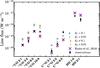 |
Fig. 13 Integrated line fluxes from TW Hya models (Mdisk = 2.3 × 10⁻²M⊙, ψ = 0.3 and hc = 0.1) with different amounts of carbon depletion (hexagons; left side) and oxygen depletion (right side). The black bars show the observations for TW Hya (Schwarz et al. 2016; Kama et al. 2016b, and references therein). The purple crosses show the results from Kama et al. (2016b), recalculated for δC = δO = 0.01, [D]/[H] = 2 × 10⁻⁵ (cf. Sect. 4.4). |
Figure 13 shows the resulting line fluxes for several rotational transitions of HD, 13CO, and C18O, similar to Fig. 6 in Kama et al. (2016b). In the figure only the models with X(C,O) ~ 10-6,10-5 are shown. The full figure can be found in Appendix E. The HD abundance used in Kama et al. (2016b) (n(HD) /n(H2) = 1 × 10⁻⁵) is a factor four lower than the maximal HD abundance of the models in this work (n(HD) /n(H2) = 4 × 10⁻⁵). In order to compare the output of the chemical calculations to their parametric method, the HD line fluxes of their model were recalculated with the higher HD abundance. This accounts for the differences in the HD line fluxes seen here and those in Kama et al. (2016b). Similar steps were taken so that the δC = δO = 0.01 model and the Kama et al. (2016b) model have the same oxygen and carbon abundances.
Starting with HD, one can see that the line fluxes from the models run here, which include the deuterium chemistry network, match the line fluxes from the model with the parametric HD within a few percent (8% and 15% for HD 1–0 and HD 2–1, respectively). This can be understood from the results in Sect. 3.2, which show that all the available deuterium is locked up in HD, thus mimicking the parametric approach used by Kama et al. (2016b). We point out that all models overproduce the observed HD fluxes by a factor ~ 2, suggesting a slightly lower disk gas mass for TW Hya than that used by Kama et al. (2016b).
For 13C, there is again good agreement between the fluxes from Kama et al. (2016b) and the δC = δO = 0.01 model (its CO isotopologue counterpart). This can be understood by reactions such as the ion-molecule reaction 13C+ + 12CO ⇌13CO + 12C+ + 35 K. The forward reaction direction of this reaction is favoured at low temperatures, leading to an increased 13CO abundance, which balances out the additional decrease of 13CO due to isotope-selective photodissociation (Miotello et al. 2014).
The line fluxes of C18O of the δC = δO = 0.01 model are systematically lower than the same lines from Kama et al. (2016b). This qualitatively agrees with previous results (e.g. Visser et al. 2009; Miotello et al. 2014), but the effect is smaller than has been suggested. A possible explanation can be found in the gas mass of the disk. Miotello et al. (2014, 2016) show that for disks with Mdisk ≥ 7 × 10⁻³M⊙ freeze-out is the dominant process affecting the C18O flux, whereas isotope-selective photodissociation is more important for low mass disks (see e.g. Fig. 3 in Miotello et al. 2016).
When the models are compared to the observations to determine the carbon and oxygen underabundance the results vary based on the tracer used. The 13CO observations point to δC = 0.01, in line with the value found by Kama et al. (2016b). The observed 13CO 10–9 flux and the observations for C18O instead favour a lower underabundance of carbon between δC = 0.01 and δC = 0.1. For all CO isotopologue lines δO = 0.01 and δO = 0.1 fit the observations equally well. Combined with the lower gas mass estimates found for TW Hya, these results show that the inclusion of isotope-selective processes decreases underabundance of carbon needed to explain the observations to δC ≈ 0.1. However in this analysis only the CO isotopologues are considered, whereas the analysis in Kama et al. (2016b) also included observations of atomic carbon and atomic oxygen.
5. Conclusions
Accurately determining the amount of material in protoplanetary disks is crucial for understanding both the evolution of disks and the formation of planets in these disks. Recent observations of the rotational transitions of HD in protoplanetary disks (Bergin et al. 2013; McClure et al. 2016) have added a new possibility of tracing the disk gas mass. In this work, the robustness of HD as a tracer of the disk gas mass and its dependence on the vertical structure are investigated. The thermochemical code DALI (Bruderer et al. 2012; Bruderer 2013) was used to calculate the line fluxes for the disk models. The normal chemical network of DALI was expanded to include CO isotopologue selective chemistry, following Miotello et al. (2014). A simple D chemistry network was also implemented in DALI. A series of models was run spreading a range of disk masses (Mdisk ~ 10-5−10-1M⊙) and vertical structures (hc ~ 0.05−0.3,ψ ~ 0.1−0.5), with the large grains settled close to the midplane. From these models, the following observations can be made:
-
The HD flux increases as a power law for low mass disks(Mdisk ≤ 10-3M⊙). The fitted power-law indices are 0.8 for HD 1–0 (112 μm) and 0.5 for HD 2–1 (56 μm). These indices are less than 1.0 because of the dependence of the emission on the gas temperature. For high mass disks (Mdisk> 10-3M⊙) the HD flux scales with log 10Mdisk, which is a result of the increased line optical depth and decreased overall temperature of these disks.
-
The maximum variation in HD 1–0 flux due to the different vertical structure increases with disk mass, from 0.75 × the median flux for Mdisk ~ 10-5M⊙ up to 1.9 × the median flux for Mdisk ~ 10-1M⊙. The variation for HD 2–1 is both larger than for HD 1–0 and is less dependent on disk mass. The maximum variation of this flux is 1.9 × the median flux for Mdisk ~ 10-5M⊙, increasing to 2.8 × the median flux for Mdisk ~ 10-1M⊙.
-
The influence of the large grain population on the HD flux is less than that of the vertical structure, approximately 0.7× the median flux at Mdisk = 2.3 × 10⁻²M⊙.
-
Without making assumptions on the vertical structure of the disk, the HD 1–0 flux can be used to estimate the disk gas mass to within a factor of ~3 for low mass disks (Mdisk ≤ 10-3M⊙). For more massive disks the uncertainty in the estimated mass increases to more than an order of magnitude.
-
If complementary observations are employed to constrain the flaring of the disk, the uncertainty on the gas mass can be reduced down to factor of 2, even for massive disks. Moreover, a combination of HD 1–0 and the HD 2–1 fluxes can be used to a determine the disk gas mass to within a factor of 3, without making assumptions on the vertical structure.
-
For DM Tau and GM Aur, gas mass estimates found by comparing the observed fluxes to the models agree with the results from McClure et al. (2016), confirming the high gas masses of these disks.
-
For TW Hya, a gas mass between 6 × 10⁻³M⊙ ≤ Mdisk ≤ 9 × 10⁻³M⊙ is found if the best fit vertical structure from (Kama et al. 2016b) is assumed. This estimate agrees with the combination of HD 1–0 and HD 2–1 line fluxes, which favour a gas mass of 7.7 × 10⁻³M⊙.
-
Detailed modelling of the TW Hya disk shows that the difference between HD- and CO-based gas masses is mitigated by including CO isotopologue selective effects. A carbon underabundance of ~ 10 with respect to the ISM can also explain the CO isotopologue observations.
In the interest of future far-infrared observatories, the line-to-continuum ratios for HD 1–0 and HD 2–1 were calculated for different spectral resolving power. If a maximum S/N on the continuum of 300 is assumed, it was shown that future far-IR missions need a spectral resolving power R ≥ 300 (equivalent to Δv ≤ 500 km s-1) to detect HD 1–0 for all disk masses. To detect HD 2–1 towards all models, a spectral resolving power of R ≥ 1000 (equivalent to Δv ≤ 150 km s-1) is required. Furthermore, a 5σ sensitivity of 1.8 × 10⁻²⁰ W m-2 (2.5 × 10⁻²⁰ W m-2) is required to detect HD 1–0 (2–1) in disks with gas mass ≥ 3 × 10⁻⁵M⊙ ≈ 0.03 Mjup. Both requirements can be met by proposed future missions such as SPICA.
Acknowledgments
The authors would like to thank Inga Kamp and Ted Bergin for the useful discussions and for providing the details about the SPICA SAFARI and SOFIA HIRMES instruments. They also acknowledge Arthur Bosman for his support with the DALI code and Davide Fedele for providing the HD 2–1 line flux that was observed for TW Hya. Astrochemistry in Leiden is supported by the Netherlands Research School for Astronomy, by a Royal Netherlands Academy of Arts and Sciences (KNAW) professor prize, and by the European Union A-ERC grant 291141 CHEMPLAN.
References
- Aikawa, Y., Umebayashi, T., Nakano, T., & Miyama, S. M. 1997, ApJ, 486, L51 [NASA ADS] [CrossRef] [Google Scholar]
- Andrews, S. M., Wilner, D. J., Espaillat, C., et al. 2011, ApJ, 732, 42 [NASA ADS] [CrossRef] [Google Scholar]
- Andrews, S. M., Wilner, D. J., Hughes, A., et al. 2012, ApJ, 744, 162 [NASA ADS] [CrossRef] [Google Scholar]
- Andrews, S. M., Rosenfeld, K. A., Kraus, A. L., & Wilner, D. J. 2013, ApJ, 771, 129 [NASA ADS] [CrossRef] [Google Scholar]
- Ansdell, M., Williams, J. P., van der Marel, N., et al. 2016, ApJ, 828, 46 [Google Scholar]
- Armitage, P. J. 2015, ArXiv e-prints [arXiv:1509.06382] [Google Scholar]
- Astraatmadja, T. L., & Bailer-Jones, C. A. L. 2016, ApJ, 833, 119 [NASA ADS] [CrossRef] [Google Scholar]
- Beckwith, S. V. W., Sargent, A. I., Chini, R. S., & Guesten, R. 1990, AJ, 99, 924 [NASA ADS] [CrossRef] [Google Scholar]
- Bergin, E., Hogerheijde, M., Brinch, C., et al. 2010, A&A, 521, L33 [NASA ADS] [CrossRef] [EDP Sciences] [Google Scholar]
- Bergin, E., Cleeves, L. I., Crockett, N., & Blake, G. 2014, Faraday discussions, 168, 61 [Google Scholar]
- Bergin, E. A., Cleeves, L. I., Gorti, U., et al. 2013, Nature, 493, 644 [NASA ADS] [CrossRef] [PubMed] [Google Scholar]
- Bergin, E. A., Du, F., Cleeves, L. I., et al. 2016, ApJ, 831, 101 [NASA ADS] [CrossRef] [Google Scholar]
- Bruderer, S. 2013, A&A, 559, A46 [NASA ADS] [CrossRef] [EDP Sciences] [Google Scholar]
- Bruderer, S., van Dishoeck, E. F., Doty, S. D., & Herczeg, G. J. 2012, A&A, 541, A91 [NASA ADS] [CrossRef] [EDP Sciences] [Google Scholar]
- Carmona, A., van der Plas, G., van den Ancker, M. E., et al. 2011, A&A, 533, A39 [NASA ADS] [CrossRef] [EDP Sciences] [Google Scholar]
- Chiang, E. I., & Goldreich, P. 1997, ApJ, 490, 368 [NASA ADS] [CrossRef] [Google Scholar]
- Chiang, E. I., Joung, M. K., Creech-Eakman, M. J., et al. 2001, ApJ, 547, 1077 [NASA ADS] [CrossRef] [Google Scholar]
- Cleeves, L. I., Bergin, E. A., Qi, C., Adams, F. C., & Öberg, K. I. 2015, ApJ, 799, 204 [NASA ADS] [CrossRef] [Google Scholar]
- D’Alessio, P., Calvet, N., & Hartmann, L. 2001, ApJ, 553, 321 [NASA ADS] [CrossRef] [Google Scholar]
- Dartois, E., Dutrey, A., & Guilloteau, S. 2003, A&A, 399, 773 [NASA ADS] [CrossRef] [EDP Sciences] [Google Scholar]
- Dent, W. R. F., Greaves, J. S., & Coulson, I. M. 2005, MNRAS, 359, 663 [NASA ADS] [CrossRef] [Google Scholar]
- Du, F., Bergin, E. A., & Hogerheijde, M. R. 2015, ApJ, 807, L32 [NASA ADS] [CrossRef] [Google Scholar]
- Dutrey, A., Guilloteau, S., Duvert, G., et al. 1996, A&A, 309, 493 [NASA ADS] [Google Scholar]
- Eistrup, C., Walsh, C., & van Dishoeck, E. F. 2016, A&A, 595, A83 [NASA ADS] [CrossRef] [EDP Sciences] [Google Scholar]
- Favre, C., Cleeves, L. I., Bergin, E. A., Qi, C., & Blake, G. A. 2013, ApJ, 776, L38 [NASA ADS] [CrossRef] [Google Scholar]
- Glover, S., & Jappsen, A.-K. 2007, AJ, 666, 1 [NASA ADS] [CrossRef] [Google Scholar]
- Hartmann, L. 2000, Accretion processes in star formation (Cambridge University Press), 32 [Google Scholar]
- Hartmann, L., Calvet, N., Gullbring, E., & D’Alessio, P. 1998, ApJ, 495, 385 [NASA ADS] [CrossRef] [Google Scholar]
- Hildebrand, R. H. 1983, QJRAS, 24, 267 [NASA ADS] [Google Scholar]
- Hogerheijde, M. R., Bergin, E. A., Brinch, C., et al. 2011, Science, 334, 338 [NASA ADS] [CrossRef] [PubMed] [Google Scholar]
- Howat, S. K. R., Timmermann, R., Geballe, T. R., Bertoldi, F., & Mountain, C. M. 2002, ApJ, 566, 905 [NASA ADS] [CrossRef] [Google Scholar]
- Kama, M., Bruderer, S., Carney, M., et al. 2016a, A&A, 588, A108 [NASA ADS] [CrossRef] [EDP Sciences] [Google Scholar]
- Kama, M., Bruderer, S., van Dishoeck, E. F., et al. 2016b, A&A, 592, A83 [NASA ADS] [CrossRef] [EDP Sciences] [Google Scholar]
- Kenyon, S. J., & Hartmann, L. 1987, ApJ, 323, 714 [NASA ADS] [CrossRef] [Google Scholar]
- Lacy, J., Knacke, R., Geballe, T., & Tokunaga, A. 1994, ApJ, 428, L69 [NASA ADS] [CrossRef] [Google Scholar]
- Lynden-Bell, D., & Pringle, J. E. 1974, MNRAS, 168, 603 [NASA ADS] [CrossRef] [Google Scholar]
- Mannings, V., & Sargent, A. I. 1997, ApJ, 490, 792 [NASA ADS] [CrossRef] [Google Scholar]
- McClure, M. K., Bergin, E. A., Cleevs, L. I., et al. 2016, ApJ, 831, 167 [NASA ADS] [CrossRef] [Google Scholar]
- Miotello, A., Bruderer, S., & van Dishoeck, E. F. 2014, A&A, 572, A96 [NASA ADS] [CrossRef] [EDP Sciences] [Google Scholar]
- Miotello, A., van Dishoeck, E. F., Kama, M., & Bruderer, S. 2016, A&A, 594, A85 [NASA ADS] [CrossRef] [EDP Sciences] [Google Scholar]
- Miotello, A., van Dishoeck, E., Williams, J., et al. 2017, A&A, 599, A113 [NASA ADS] [CrossRef] [EDP Sciences] [Google Scholar]
- Müller, H. S. P., Schlöder, F., Stutzki, J., & Winnewisser, G. 2005, J. Mol. Struct., 742, 215 [NASA ADS] [CrossRef] [Google Scholar]
- Nakagawa, T., Shibai, H., Onaka, T., et al. 2014, in Proc. SPIE, 9143, 91431I [Google Scholar]
- Panić, O., Hogerheijde, M. R., Wilner, D., & Qi, C. 2008, A&A, 491, 219 [NASA ADS] [CrossRef] [EDP Sciences] [Google Scholar]
- Pascucci, I., Herczeg, G., Carr, J., & Bruderer, S. 2013, AJ, 779, 178 [Google Scholar]
- Prodanović, T., Steigman, G., & Fields, B. D. 2010, MNRAS, 406, 1108 [NASA ADS] [Google Scholar]
- Roberts, H., & Millar, T. 2000, A&A, 361, 388 [NASA ADS] [Google Scholar]
- Roelfsema, P., Giard, M., Najarro, F., et al. 2014, in Proc. SPIE, 9143, 91431K [Google Scholar]
- Schwarz, K. R., Bergin, E. A., Cleeves, L. I., et al. 2016, AJ, 823, 91 [Google Scholar]
- Thi, W. F., van Dishoeck, E. F., Blake, G. A., et al. 2001, ApJ, 561, 1074 [NASA ADS] [CrossRef] [Google Scholar]
- van Zadelhoff, G.-J., van Dishoeck, E. F., Thi, W.-F., & Blake, G. A. 2001, A&A, 377, 566 [NASA ADS] [CrossRef] [EDP Sciences] [Google Scholar]
- Visser, R., van Dishoeck, E. F., & Black, J. H. 2009, A&A, 503, 323 [NASA ADS] [CrossRef] [EDP Sciences] [Google Scholar]
- Walmsley, C. M., Flower, D., & Des Forêts, G. P. 2004, A&A, 418, 1035 [NASA ADS] [CrossRef] [EDP Sciences] [Google Scholar]
- Weingartner, J. C., & Draine, B. 2001, ApJ, 548, 296 [NASA ADS] [CrossRef] [Google Scholar]
- Williams, J. P., & Best, W. M. J. 2014, ApJ, 788, 59 [NASA ADS] [CrossRef] [Google Scholar]
- Williams, J. P., Andrews, S. M., & Wilner, D. J. 2005, ApJ, 634, 495 [NASA ADS] [CrossRef] [Google Scholar]
- Woitke, P., Kamp, I., & Thi, W.-F. 2009, A&A, 501, 383 [NASA ADS] [CrossRef] [EDP Sciences] [Google Scholar]
- Wright, C. M., van Dishoeck, E. F., Cox, P., Sidher, S. D., & Kessler, M. F. 1999, ApJ, 515, L29 [NASA ADS] [CrossRef] [Google Scholar]
Appendix A: Abundance and temperature maps of TW Hya
In Fig. A.1 the abundance maps of 13CO and C18O are shown for the TW Hya model (Mdisk = 2.3 × 10⁻²M⊙, hc = 0.1, ψ = 0.3 and δC = δO = 0.01). The gas and dust temperature structures for the same model are shown in the panels of Fig. A.2.
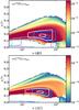 |
Fig. A.1 Maps of the 13CO (top) and C18O (bottom) abundances. The coloured lines correspond to xCyO 2–1 (blue), 3–2 (light blue), and 6–5 (white), respectively. The solid lines denote where 25% and 75% of the emission is produced. the dashed lines. The dashed lines show the τ = 1 surface for the line emission. The dash-dotted lines show the τ = 1 surface for the continuum at the wavelength of the line. |
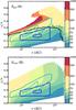 |
Fig. A.2 Maps of the gas temperature (top) and dust temperature (bottom). The solid lines denote where 25% and 75% of the emission from HD 1–0 (blue) and HD 2–1 (light blue) originate from. The region below the black line in the top panel is where Tgas = Tdust. |
Appendix B: Abundance and emission maps of grid models
The HD abundance maps for several models with different vertical structures and disk masses are shown here. Figure B.1 presents four models with different vertical structures: (hc,ψ) = [0.05,0.1] , [0.05,0.5] , [0.3,0.1] , [0.3,0.5]. These represent the most extreme cases in the grid. The top and bottom rows in the figure have different vertical extents. Also note that the HD 1–0 emission (blue solid contours) originates from approximately the same horizontal region in all four models, between a few AU and several tens of AU.
Figure B.2 presents the abundance maps for three disks with different disk masses: Mdisk = [10-5,10-3,10-1] M⊙; the height τ = 1 surface for the line optical depth (blue dashed line) increases with disk mass.
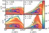 |
Fig. B.1 Maps of the HD abundance for four models with different vertical structures. Starting with the top left figure and continuing clockwise the vertical structures shown are (hc,ψ) = [0.05,0.1] , [0.05,0.5] , [0.3,0.1] , [0.3,0.5]. The top and bottom rows have different ranges on the vertical axis. The solid lines denote where 25% and 75% of the emission from HD 1–0 (blue) and HD 2–1 (light blue) originate from. |
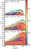 |
Fig. B.2 Maps of the HD abundance for three models with different disk masses: Mdisk = [10-5,10-3,10-1] M⊙. The solid lines denote where 25% and 75% of the emission from HD 1–0 (blue) and HD 2–1 (light blue) originate from. |
Appendix C: Effects of including hydrostatic equilibrium
As shown in Fig. 3, the HD emission originates from regions close to the disk surface. Accordingly, the HD emission depends on the assumed disk vertical structure. In the models presented here the vertical structure is parametrized with a Gaussian (cf. Eq. (2)), to mimic a balance between gravitational force and pressure gradient, which in reality would depend on the temperature structure of the disk. Another possible approach is to derive the vertical structure with the hydrostatic equilibrium (e.g. Woitke et al. 2009). This results in a puffed-up inner rim, which shadows the outer disk from direct irradiation by the star. However, this may be a temporary feature that could be dispersed by, for instance stellar winds.
For completeness, we have investigated how the inclusion of hydrostatic equilibrium would affect the HD emission. The fiducial model described in Sect. 3.2 was rerun using eight iterations of the hydrostatic solver of DALI, where the temperature structure of the (n−1)th model is used to calculate the vertical structure of the nth model. The resulting vertical structure is then used to recalculate the dust and gas temperatures, chemistry, and HD emissions.
Appendix C.1: Hydrostatic solver
One way to obtain the vertical structure of the disk is to solve the equations of hydrostatic equilibrium. The hydrostatic equations in cylindrical geometry read (e.g. Hartmann 2000)  where the velocities in the z and r direction are assumed to be 0. Without self-gravity, the gravitational potential by the star is
  (C.3)where M∗ is the mass of the star.
Assuming that the pressure gradient in the r direction is negligible, the first hydrostatic equation yields the Keplerian velocity profile and the second hydrostatic equation can be solved independently for each radius. Instead of directly solving the equation for the density ρ, the equation can also be solved for
pressure. The pressure and density are related through  , where cs is the sound speed that depends on the gas temperature Tgas and therefore varies with height z. The differential equation for P reads
  which is solved by
  (C.6)In the case of an isothermal disk, the above equation reduces to a Gaussian vertical density profile, as given in Eq. (2). The integration constant C in the above equation results from the normalization conditions for the vertical column density and should thus adjusted such that ∫ρ(z)dz is preserved.
Appendix C.2: Comparing with parametrized vertical structure
Figure C.1 shows the effect of eight iterations of the hydrostatic solver on the density and gas temperature structure of the fiducial model (Mdisk = 2.3 × 10⁻²M⊙, ψ = 0.3 and hc = 0.1; cf. Sect. 3.2). It also shows the regions where the HD 1–0 emission is produced before and after applying the hydrostatic solver. The top panel shows that the HD 1–0 emission has moved slightly towards the midplane for the hydrostatic model. This is likely the result of the decrease in height of the line optical depth surface. The bottom panel shows that the gas temperature in the HD 1–0 emitting region has changed by less than 5%.
The effect of the hydrostatic solver on the HD emitting regions is shown in Fig. C.2. While disk models obtained with the hydrostatic calculations are vertically more extended, the HD emitting regions have not extremely changed. This is also reflected in the integrated fluxes, which for the hydrostatic model are ~ 50% (HD 1–0) and ~ 66% (HD 2–1) lower compared to the model with the parametrized vertical structure. While this affects the inferred disk masses by a similar absolute factor, all the trends presented here should be robust. Also varying the parametric vertical structure changes the HD fluxes by a similar or larger factor (cf. Fig. 4). The mass uncertainties calculated in Sect. 4.1 therefore remain unchanged.
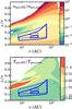 |
Fig. C.1 Maps of the density (top) and temperature (bottom) differences between the fiducial model (denoted “para”; Sect. 3.2) and the same model after eight iterations of the hydrostatic solver (denoted “HE”). Colour indicates the ratio of the densities or gas temperatures of the two models. The dashed blue lines show the HD 1–0 emitting region of the fiducial model. The solid blue lines show the HD 1–0 the 25% and 75% cumulative emission regions of the “HE” model. |
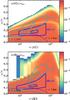 |
Fig. C.2 Top panel: HD abundance structure for a disk model, with Mdisk = 2.3×10⁻²M⊙, ψ = 0.3 and hc = 0.1, which is identical to Fig. 3. Colour indicates the number density of HD with respect to the total gas density. The coloured lines correspond the HD 1–0 (blue) and HD 2–1 (light blue), respectively. Solid contours indicate where 25% and 75% of the emission originates from. The dashed (dash-dotted) lines show the τ = 1 surface for the line and continuum opacity, respectively. Bottom panel: HD abundance structure of the same initial model, where the vertical structure is now determined by eight iterations of the hydrostatic solver of DALI. |
Appendix D: Deuterium chemistry
Table D.1 list the reactions that were included in the deuterium chemical network. The rate coefficients were adapted
from Roberts & Millar (2000), Walmsley et al. (2004), and Glover & Jappsen (2007). Where the rate coefficients were not known, the coefficients for the analogue reactions with H instead of D were used.
Simple HD chemical network reactions and adopted rate coefficient.
Appendix E: Line fluxes of the TW Hya model
The extended version of Fig. 13 is shown here. Its setup is similar to Fig. 6 in Kama et al. (2016b). The fluxes and upper limits for the observations used can be found in Table B.1 in Kama et al. (2016b). The line fluxes of 13CO 6–5, C18O 3–2, and C18O 6–5 were calculated from the data presented in Schwarz et al. (2016).
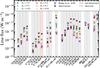 |
Fig. E.1 Integrated line fluxes from TW Hya models (Mdisk = 2.3 × 10⁻²M⊙, ψ = 0.3, hc = 0.1, d = 59.54 pc, Astraatmadja & Bailer-Jones 2016) with different amounts of carbon/oxygen underabundances. The x-axis shows the various modelled transitions. The black bars show the observations for TW Hya (Schwarz et al. 2016; Kama et al. 2016b, and references therein). The purple crosses show the modelled line fluxes from the best fit model from Kama et al. (2016b; with δC = δO = 0.01). The coloured hexagons show the results from this work; the left-hand side shows the amount carbon underabundance (with respect to the ISM) and the right-hand side shows the amount of oxygen underabundance. |
All Tables
All Figures
|
Fig. 1 Gas and dust density structure assumed in DALI. |
| In the text | |
|
Fig. 2 Left panel: integrated line flux (calculated at 140 pc) of the HD 1–0 transition as a function of disk mass. The points show the median flux of the models in that mass bin. The blue shaded region shows fluxes between the 16th and 84th percentiles in the same mass bin. The blue line shows the fit of Eq. (6)using the values from Table 3. Right panel: integrated line flux (calculated at 140 pc) of the HD 2–1 transition as a function of disk mass. |
| In the text | |
|
Fig. 3 HD abundance structure for a disk model with Mdisk = 2.3 × 10⁻²M⊙, ψ = 0.3 and hc = 0.1. Colour indicates the number density of HD with respect to the total gas density. The coloured lines correspond the HD 1–0 (blue) and HD 2–1 (light blue), respectively. Solid contours indicate where 25% and 75% of the emission originates from. The dashed (dash-dotted) lines show the τ = 1 surface for the line and continuum opacity, respectively. |
| In the text | |
|
Fig. 4 Integrated HD 1–0 (top) and HD 2–1 (bottom) line fluxes as functions of flaring angle ψ for different scale heights hc. The fluxes are normalized with respect to median flux of the models with the same disk mass (cf. Fig. 2). |
| In the text | |
|
Fig. 5 Integrated line flux of HD 1–0 as a function of dust parameters for Mdisk = 2.3×10⁻²M⊙. Models with different flarge and χ are shown in orange and green, respectively. The fluxes are normalized to the median flux of the Mdisk = 2.3 × 10⁻²M⊙ mass bin. The triangular marker denotes the value of the parameter (flarge or χ) in the fiducial model of the TW Hya disk (Kama et al. 2016b; cf. Table 2). |
| In the text | |
|
Fig. 6 Integrated line flux of HD 1–0 as a function of the gas-to-dust mass ratio for fixed gas mass (Mgas = 2.3 × 10⁻²M⊙). The fluxes are normalized to the median flux of the Mdisk = 2.3 × 10⁻²M⊙ mass bin. The triangular marker denotes the value of Δgd in the fiducial model of the TW Hya disk (Kama et al. 2016b; cf. Table 2). |
| In the text | |
|
Fig. 7 HD 1–0 integrated fluxes and 870 μm continuum flux densities for the models described in Table 4. Colours indicate various gas-to-dust ratios, where the shaded region shows the flux variations from different vertical structures. For each Δgd, the coloured line shows models with (ψ,hc) = (0.3, 0.1). The crosses denote observations for TW Hya (black; Bergin et al. 2013; Andrews et al. 2012), DM Tau (purple; McClure et al. 2016; Andrews et al. 2013) and GM Aur (green; McClure et al. 2016; Andrews et al. 2013). Both the model fluxes and the observations were scaled to a distance of 140 pc. |
| In the text | |
|
Fig. 8 Line-to-continuum ratios of HD as functions of Mdisk for different spectral resolving powers. The points show the median L/C of the models in the mass bin. The shaded region shows the L/Cs between the 16th and 84th percentile in each mass bin. The red line represents a 3σ detection limit of L/C= 0.01, which is equivalent to assuming a S/N on the continuum of 300. |
| In the text | |
|
Fig. 9 HD 1–0 (blue) and 2–1 (green) model fluxes (calculated at 140 pc) as functions of disk gas mass (cf. Fig. 2). The horizontal lines represent the 5σ sensitivities for various instruments. The solid lines show the detection limit after 1 h of integration. The dashed lines show the 5σ sensitivity at 112 μm after 10 h of integration (labelled “deep survey”). |
| In the text | |
|
Fig. 10 Calculated mass uncertainties (cf. Eq. (8)) as functions of HD 1–0 flux. The left and right vertical axis are related via ΔMfactor = 10ΔMdex. The black line shows the result if the full set of models is used (cf. Table 2). The other three lines show results for weakly flared (purple), intermediately flared (orange) and strongly flared (light green) disks (see Table 5 for definitions for these subsets). The subsets are also shown in the top left panel, which shows a scaled version of Fig. 2. |
| In the text | |
|
Fig. 11 HD 1–0 and HD 2–1 integrated fluxes (calculated at 140 pc) for the models described in Sect. 2.4. The different colours indicate different disk masses. The observations for TW Hya are shown in black (Bergin et al. 2013; Kama et al. 2016b; D. Fedele, priv. comm.). The bottom right corner shows the region around the observations, where the shaded regions link models that are within the same mass bin. |
| In the text | |
|
Fig. 12 Integrated line flux (calculated at 140 pc) of the HD 1–0 transition as a function of disk mass, representing the high mass end of the left panel of Fig. 2. The horizontal black solid line gives the observation of TW Hya, scaled to a distance of 140 pc, with the black shaded region representing the 1σ uncertainties (Bergin et al. 2013). The observations for DM Tau and GM Aur (McClure et al. 2016) are shown in purple and green, respectively. |
| In the text | |
|
Fig. 13 Integrated line fluxes from TW Hya models (Mdisk = 2.3 × 10⁻²M⊙, ψ = 0.3 and hc = 0.1) with different amounts of carbon depletion (hexagons; left side) and oxygen depletion (right side). The black bars show the observations for TW Hya (Schwarz et al. 2016; Kama et al. 2016b, and references therein). The purple crosses show the results from Kama et al. (2016b), recalculated for δC = δO = 0.01, [D]/[H] = 2 × 10⁻⁵ (cf. Sect. 4.4). |
| In the text | |
|
Fig. A.1 Maps of the 13CO (top) and C18O (bottom) abundances. The coloured lines correspond to xCyO 2–1 (blue), 3–2 (light blue), and 6–5 (white), respectively. The solid lines denote where 25% and 75% of the emission is produced. the dashed lines. The dashed lines show the τ = 1 surface for the line emission. The dash-dotted lines show the τ = 1 surface for the continuum at the wavelength of the line. |
| In the text | |
|
Fig. A.2 Maps of the gas temperature (top) and dust temperature (bottom). The solid lines denote where 25% and 75% of the emission from HD 1–0 (blue) and HD 2–1 (light blue) originate from. The region below the black line in the top panel is where Tgas = Tdust. |
| In the text | |
|
Fig. B.1 Maps of the HD abundance for four models with different vertical structures. Starting with the top left figure and continuing clockwise the vertical structures shown are (hc,ψ) = [0.05,0.1] , [0.05,0.5] , [0.3,0.1] , [0.3,0.5]. The top and bottom rows have different ranges on the vertical axis. The solid lines denote where 25% and 75% of the emission from HD 1–0 (blue) and HD 2–1 (light blue) originate from. |
| In the text | |
|
Fig. B.2 Maps of the HD abundance for three models with different disk masses: Mdisk = [10-5,10-3,10-1] M⊙. The solid lines denote where 25% and 75% of the emission from HD 1–0 (blue) and HD 2–1 (light blue) originate from. |
| In the text | |
|
Fig. C.1 Maps of the density (top) and temperature (bottom) differences between the fiducial model (denoted “para”; Sect. 3.2) and the same model after eight iterations of the hydrostatic solver (denoted “HE”). Colour indicates the ratio of the densities or gas temperatures of the two models. The dashed blue lines show the HD 1–0 emitting region of the fiducial model. The solid blue lines show the HD 1–0 the 25% and 75% cumulative emission regions of the “HE” model. |
| In the text | |
|
Fig. C.2 Top panel: HD abundance structure for a disk model, with Mdisk = 2.3×10⁻²M⊙, ψ = 0.3 and hc = 0.1, which is identical to Fig. 3. Colour indicates the number density of HD with respect to the total gas density. The coloured lines correspond the HD 1–0 (blue) and HD 2–1 (light blue), respectively. Solid contours indicate where 25% and 75% of the emission originates from. The dashed (dash-dotted) lines show the τ = 1 surface for the line and continuum opacity, respectively. Bottom panel: HD abundance structure of the same initial model, where the vertical structure is now determined by eight iterations of the hydrostatic solver of DALI. |
| In the text | |
|
Fig. E.1 Integrated line fluxes from TW Hya models (Mdisk = 2.3 × 10⁻²M⊙, ψ = 0.3, hc = 0.1, d = 59.54 pc, Astraatmadja & Bailer-Jones 2016) with different amounts of carbon/oxygen underabundances. The x-axis shows the various modelled transitions. The black bars show the observations for TW Hya (Schwarz et al. 2016; Kama et al. 2016b, and references therein). The purple crosses show the modelled line fluxes from the best fit model from Kama et al. (2016b; with δC = δO = 0.01). The coloured hexagons show the results from this work; the left-hand side shows the amount carbon underabundance (with respect to the ISM) and the right-hand side shows the amount of oxygen underabundance. |
| In the text | |
Current usage metrics show cumulative count of Article Views (full-text article views including HTML views, PDF and ePub downloads, according to the available data) and Abstracts Views on Vision4Press platform.
Data correspond to usage on the plateform after 2015. The current usage metrics is available 48-96 hours after online publication and is updated daily on week days.
Initial download of the metrics may take a while.