| Issue |
A&A
Volume 603, July 2017
|
|
|---|---|---|
| Article Number | A96 | |
| Number of page(s) | 20 | |
| Section | Interstellar and circumstellar matter | |
| DOI | https://doi.org/10.1051/0004-6361/201630241 | |
| Published online | 12 July 2017 | |
Stellar energetic particle ionization in protoplanetary disks around T Tauri stars
1 University of Vienna, Dept. of Astrophysics, Türkenschanzstr. 17, 1180 Wien, Austria
e-mail: This email address is being protected from spambots. You need JavaScript enabled to view it.
2 INAF-Ossevatorio Astrofisico di Arcetri, Largo E. Fermi, 5, 50125 Firenze, Italy
3 Kapteyn Astronomical Institute, University of Groningen, PO Box 800, 9700 AV Groningen, The Netherlands
4 Max-Planck-Institut für extraterrestrische Physik, Giessenbachstrasse 1, 85748 Garching, Germany
5 SUPA, School of Physics & Astronomy, University of St. Andrews, North Haugh, St. Andrews KY16 9SS, UK
6 INAF, Osservatorio Astronomico di Cagliari, via della Scienza 5, 09047 Selargius, Italy
Received: 13 December 2016
Accepted: 23 February 2017
Abstract
Context. Anomalies in the abundance measurements of short lived radionuclides in meteorites indicate that the protosolar nebulae was irradiated by a large number of energetic particles (E ≳ 10 MeV). The particle flux of the contemporary Sun cannot explain these anomalies. However, similar to T Tauri stars the young Sun was more active and probably produced enough high energy particles to explain those anomalies.
Aims. We aim to study the interaction of stellar energetic particles with the gas component of the disk (i.e. ionization of molecular hydrogen) and identify possible observational tracers of this interaction.
Methods. We used a 2D radiation thermo-chemical protoplanetary disk code to model a disk representative for T Tauri stars. We used a particle energy distribution derived from solar flare observations and an enhanced stellar particle flux proposed for T Tauri stars. For this particle spectrum we calculated the stellar particle ionization rate throughout the disk with an accurate particle transport model. We studied the impact of stellar particles for models with varying X-ray and cosmic-ray ionization rates.
Results. We find that stellar particle ionization has a significant impact on the abundances of the common disk ionization tracers HCO+ and N2H+, especially in models with low cosmic-ray ionization rates (e.g. 10-19 s-1 for molecular hydrogen). In contrast to cosmic rays and X-rays, stellar particles cannot reach the midplane of the disk. Therefore molecular ions residing in the disk surface layers are more affected by stellar particle ionization than molecular ions tracing the cold layers and midplane of the disk.
Conclusions. Spatially resolved observations of molecular ions tracing different vertical layers of the disk allow to disentangle the contribution of stellar particle ionization from other competing ionization sources. Modelling such observations with a model like the one presented here allows to constrain the stellar particle flux in disks around T Tauri stars.
Key words: stars: formation / circumstellar matter / stars: activity / radiative transfer / astrochemistry / methods: numerical
© ESO, 2017
1. Introduction
Our Sun acts as a particle accelerator and produces energetic particles with energies ≥10 MeV (e.g. Mewaldt et al. 2007). Such particles are also called solar cosmic rays as their energies are comparable to Galactic cosmic rays. They are accelerated in highly violent events like flares and/or close to the solar surface due to shocks produced by coronal mass ejections (Reames 2015). Therefore the energetic particle flux is strongly correlated with the activity of the Sun (e.g. Mewaldt et al. 2005; Reedy 2012).
From X-ray observations of T Tauri stars we know that their X-ray luminosities can be up to 104 times higher than the X-ray luminosity of the contemporary Sun (e.g. Feigelson & Montmerle 1999; Güdel et al. 2007). Such high X-ray luminosities are rather a result of enhanced flare activity of young stars than coronal effects (e.g Feigelson et al. 2002). Enhanced activity of T Tauri stars implies an increase of their stellar energetic particle (SP) flux. From simple scaling with the X-ray luminosity and considering that young stars produce more powerful flares, Feigelson et al. (2002) derived a typical SP flux for T Tauri stars ≈105 times higher than for the contemporary Sun. Under these assumptions T Tauri stars might show on average a continuous proton flux of fp(Ep ≥ 10 MeV) ≈ 107 protons cm-2 s-1 at a distance of 1 au from the star.
Such a scenario is also likely for the young Sun. Measurements of decay products of short-lived radionuclides (SLR) like 10Be or 26Al in meteorites indicate an over-abundance of SLRs in the early phases of our solar system (e.g. Meyer & Clayton 2000). One likely explanation for these abundance anomalies are spallation reactions of SPs with the dust in the protosolar nebula (e.g. Lee et al. 1998b; McKeegan et al. 2000; Gounelle et al. 2001, 2006). However, this would require a strongly enhanced SP flux of the young Sun by a factor ≳3 × 10⁵ compared to the contemporary Sun (McKeegan et al. 2000), consistent with the estimated SP flux of T Tauri stars derived by Feigelson et al. (2002).
More recently Ceccarelli et al. (2014) reported a first indirect measurement of SPs in the protostar OMC-2 FIR 4. They observed a low HCO+/N2H+ abundance ratio between three and four that requires high H2 ionization rates >10-14 s-1 throughout the protostellar envelope. They explain this high ionization rate by the presence of SPs. From this ionization rate they derived a particle flux of fp(Ep ≥ 10 MeV) ≥ 3 − 9 × 10¹¹ protons cm-2 s-1 at 1 au distance from the star. Such a high flux would be more than sufficient to explain the over-abundance of SLRs in the solar nebula.
A further indication of SPs in young stars is the anti-correlation of X-ray fluxes with the crystalline mass fraction of the circumstellar dust found by Glauser et al. (2009). They argue that SPs are responsible for the amorphization of dust particles and that the correlation can be explained if the SP flux scales with the stellar X-ray luminosity. Trappitsch & Ciesla (2015) tested such a scenario by using detailed models of SP transport for a protoplanetary disk (i.e. SP flux as a function of height of the disk). They also considered the vertical “mixing” of dust particles. According to their models SP irradiation of the disk cannot explain the total SLR abundances in the solar nebula but might play a role for dust amorphization.
Like Galactic cosmic rays SPs not only interact with the solid component but also with the gas component of the disk. However, little is known about the impact of SPs on the chemical structure of disks. Turner & Drake (2009) investigated the relevance of SPs on the size of dead-zones in disks. Assuming similar enhancement factors as mentioned above they find that SPs can decrease the size of the dead zone depending on the disk model and other ionization sources.
We present a first approach to study the impact of SP ionization on the chemical structure of the disk. We assume a typical SP flux as proposed for T Tauri stars to study the impact of SP ionization on the common disk ionization tracers HCO+ and N2H+. We use the radiation thermo-chemical disk model PRODIMO (PROtoplanetary DIsk MOdel, Woitke et al. 2009, 2016; Kamp et al. 2010; Thi et al. 2011) to model the thermal and chemical structure of the disk. We argue that spatially resolved radial intensity profiles of molecular ion emission of the disk allow to constrain the SP flux of T Tauri stars.
In Sect. 2 we describe our method to derive the ionization rate due to SPs and the disk model. Our results are presented in Sect. 3 where we show the impact of SPs on the common disk ionization tracers HCO+ and N2H+. In Sect. 4 we discuss possibilities to constrain the SP flux via observations of molecular ion emission and future prospects for modelling of SP ionization in protoplanetary disks. We present a summary and our main conclusions in Sect. 5.
2. Method
To investigate the impact of SPs on the disk chemical structure we first needed to determine the SP flux and the particle energy distribution. With these particle spectra we were able to calculate the ionization rate throughout the disk. We applied this to a disk structure representative for disks around T Tauri stars. With the radiation thermo-chemical disk code PRODIMO we calculated the chemical abundances. We did this for a series of models in which we also considered other important high energy ionization sources like Galactic cosmic rays (CR) and X-rays.
2.1. Stellar energetic particle spectra
As the actual particle spectra and fluxes of young stars are unknown, we derived the spectra from the knowledge available from our Sun. The origin of solar energetic particles are most likely flares and/or shock waves driven by coronal-mass ejections (CME; Reames 2013, 2015). Flares act like point sources on the solar surface whereas the shock waves can fill half of the heliosphere at around 2 Solar radii (Reames 2015). Particle fluxes are not continuous but rather produced in events lasting from several hours to days (Feigelson et al. 2002; Mewaldt et al. 2005).
Based on observed X-ray luminosities of solar analogs in the Orion nebula Feigelson et al. (2002) estimated that SP fluxes in young stars are likely ≈105 times higher than in the contemporary Sun (see also Glassgold et al. 2005). As T Tauri stars are very active Feigelson et al. (2002) argue that it is likely that X-ray flares with luminosities below the detection limit occur several times a day (the same argument holds for CMEs). In that case the X-ray flares and consequently also SP events overlap, resulting in an enhanced continuous SP flux.
Based on these arguments we have assumed here a continuous and enhanced SP flux for young T Tauri stars. This approximation is consistent with the assumption of powerful and overlapping flare and CME events of T Tauri stars.
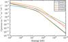 |
Fig. 1 Stellar particle (proton) spectra for five different solar particle events. Shown are fits to the measurements presented in Mewaldt et al. (2005). |
In Mewaldt et al. (2005) measurements of five different solar particle events are reported. We used their fitting formulae (see their Eq. (2) and Table 5) and derive SP spectra (protons in this case) averaged over the duration of the observed events. These measurements are for particles with energies up to several 100 MeV. We extrapolated their results up to energies typical for Galactic cosmic rays of ≈10 GeV. This is consistent with the maximum energy Emax ≈ 30 GeV derived by Padovani et al. (2015, 2016) for particles accelerated on protostellar surfaces. The resulting spectra are shown in Fig. 1. The flux levels for the different events can vary by up to two orders of magnitude and there is also some variation in the shape of the spectra.
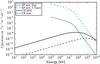 |
Fig. 2 Stellar energetic proton (SP) and cosmic-ray (CR) input spectra. The blue solid and dashed lines show the active Sun and active T Tauri SP spectrum, respectively. The black solid line shows the “LIS W98” CR spectrum from Webber (1998) and the dashed black line the attenuated “Solar Max” CR spectrum from Cleeves et al. (2013). |
Reedy (2012) reported proton fluxes of the contemporary Sun for five solar cycles. Typical values for the cycle averaged fluxes at a distance of 1 au are fp(Ep> 10 MeV) = 59 − 213 protons cm-2 s-1. For the Event1 spectrum in Fig. 1 we get fp(Ep> 10 MeV) = 151 protons cm-2 s-1 at 1 au, very similar to the reported values of Reedy (2012).
Here we used only the Event1 spectrum, which we call the “active Sun” spectrum. We simply scaled the active Sun spectrum by a factor of ≈105, as proposed by Feigelson et al. (2002), to get a typical “active T Tauri” spectrum. The resulting SP flux of fp(Ep> 10 MeV) = 1.51 × 10⁷ protons cm-2 s-1 is consistent with the value of ≈107 protons cm-2 s-1 derived by Feigelson et al. (2002) for young solar analogs in the Orion Nebula cluster. The two SP spectra are shown in Fig. 2, where we also show two cases of Galactic cosmic-ray spectra for comparison (see Sect. 2.3.2).
For comparison we also present models applying the same approach for the treatment of SPs as Turner & Drake (2009). For their model they assumed that SPs behave very similar to Galactic CRs (e.g. particle energies). The details of the Turner model are discussed in Appendix D.
It is not clear if SPs actually reach the disk (see Feigelson et al. 2002, for a discussion). However, as we are interested in the possible impact of SPs on the chemistry, we simply assumed that all SPs reach the disk. We further discuss this assumption in Sect. 4.3.
2.2. Stellar particle transport and ionization rate
Energetic particles hitting the disk interact with its gas and dust contents. Although the interaction with the solids is relevant for the production of SLR, here we are only interested in the interaction with the gas. Dust only plays a minor role in the actual attenuation of particles as only ≈1% of the mass in protoplanetary disk is in solids (see also Trappitsch & Ciesla 2015). Very similar to Galactic cosmic rays, SPs mainly ionize the gaseous medium (i.e. molecular hydrogen). Energetic particles interact multiple times and ionize many atoms and molecules on their way until they eventually have lost their energy completely. This complex process requires detailed particle transport models.
To model the transport of energetic particles through the disk gas, we used the continuous slowing down approximation, which assumes that particles lose an infinitesimal fraction of their energy during propagation (Takayanagi 1973). We used the results obtained by Padovani et al. (2009, 2013a) who compute the propagation of CRs in a 1D slab, taking all the relevant energy loss processes into account. They give a useful fitting formula for the ionization rate as a function of the column density of molecular hydrogen.
In order to apply the results of this 1D transport model, we assumed that SPs travel along straight lines (i.e. no scattering due to their high energies) and that they originate from a point source (the star). We also disregarded the effect of magnetic fields that could increase or decrease the ionization rate depending on their configuration (Padovani & Galli 2011; Padovani et al. 2013b, see also Sect. 4.3.2).
From the detailed 1D particle transport model we derived a simple fitting formulae for the two SP spectra considered here. The SP ionization rate ζSP for molecular hydrogen as a function of the total hydrogen column density N⟨ H ⟩ = NH + 2 × NH2 is given by ![Mathematical equation: \begin{equation} \zeta_\mathrm{SP}(N_\mathrm{\langle H\rangle})=\left[\frac{1}{\zeta_\mathrm{L}\left(\frac{N_\mathrm{\langle H\rangle}}{10^{20}\,\mathrm{cm^{-2}}}\right)^a} +\frac{1}{\zeta_\mathrm{H}\left(\frac{N_\mathrm{\langle H\rangle}}{10^{20}\,\mathrm{cm^{-2}}}\right)^b}\right]^{-1}\;\;\mathrm{[s^{-1}]}, \label{eqn:strcfit} \end{equation}](/articles/aa/full_html/2017/07/aa30241-16/aa30241-16-eq26.png) (1)and for N⟨ H ⟩>NE by
(1)and for N⟨ H ⟩>NE by ![Mathematical equation: \begin{equation} \zeta_\mathrm{SP,E}(N_\mathrm{\langle H \rangle})=\zeta_\mathrm{SP}(N_\mathrm{\langle H \rangle})\times\exp\left[-\left(\frac{N_\mathrm{\langle H \rangle}}{N_\mathrm{E}}-1.0\right)\right]\;\;\mathrm{[s^{-1}]}. \label{eqn:strcfitH} \end{equation}](/articles/aa/full_html/2017/07/aa30241-16/aa30241-16-eq28.png) (2)The two power laws in Eq. (1) are a consequence of the shape of the SP input spectra (see Fig. 2). The two parts of Eq. (1) account for the ionization rate at low (ζL) and high (ζH) column densities. Equation (2) accounts for the exponential drop of the SP ionization rate starting at a certain column density given by NE (i.e. similar to CRs). For the two SP spectra considered here NE = 2.5 × 1025 cm-2. The other fitting parameters ζL, ζH, a and b are given in Table 1.
(2)The two power laws in Eq. (1) are a consequence of the shape of the SP input spectra (see Fig. 2). The two parts of Eq. (1) account for the ionization rate at low (ζL) and high (ζH) column densities. Equation (2) accounts for the exponential drop of the SP ionization rate starting at a certain column density given by NE (i.e. similar to CRs). For the two SP spectra considered here NE = 2.5 × 1025 cm-2. The other fitting parameters ζL, ζH, a and b are given in Table 1.
Fitting parameters for the stellar particle ionization rate for the two different input spectra.
Equations (1) and (2) provide the unattenuated SP ionization rate at 1 au distance from the star (i.e. for a SP flux at 1 au). To account for geometric dilution we scaled ζSP(N⟨ H ⟩) by 1 /r2 at every point in the disk (r is the distance to the star in au). For the chemistry we simply added ζSP to the ionization rate for Galactic cosmic rays ζCR (see Sect. 2.3.2).
2.3. Other ionization sources
To investigate the impact of SPs on the disk ionization structure also other ionization sources common to T Tauri stars must be considered. Besides SPs our model includes stellar UV and X-ray radiation, interstellar UV radiation and Galactic cosmic rays (CRs). However, most relevant for our study are the high energy ionization sources capable of ionizing molecular hydrogen: SPs, X-rays and CRs.
2.3.1. X-rays
To model the stellar X-ray spectrum we used an approximation for an isothermal bremsstrahlung spectrum (Glassgold et al. 1997; Aresu et al. 2011) 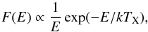 (3)where E is the photon energy (here in the range of 0.1 to 20 keV), k the Boltzmann constant and TX is the plasma temperature. This spectrum is scaled to a given total X-ray luminosity LX (0.3 ≤ E ≤ 10 keV, e.g. Güdel et al. 2010).
As a result of the activity of the stars (e.g. flares) X-ray radiation of young stars is variable. We account for this in a simple way by including a spectrum with a X-ray luminosity and temperature representative for a typical T Tauri star, and a spectrum which represents a flaring spectrum (more activity) with higher luminosity and a harder (hotter) radiation. However, we actually ignored the variability and assume time averaged X-ray fluxes. According to Ilgner & Nelson (2006) this is a reasonable assumption as typically the recombination timescales in the disk are longer than the flaring period and large parts of the disk (r ≳ 2 au in their model) respond to an enhanced average X-ray luminosity.
We also included the stellar X-ray properties used in Turner & Drake (2009) for the Turner models (Appendix D). The parameters for the various X-ray input spectra are given in Table 2 and the spectra are shown in Fig. 3.
To derive the X-ray ionization rate ζX we used X-ray radiative transfer including scattering and a detailed treatment of X-ray chemistry (Aresu et al. 2011; Meijerink et al. 2012). For more details on the new X-ray radiative transfer module in PRODIMO see Appendix A.
2.3.2. Galactic cosmic rays
Protoplanetary disks are exposed to Galactic cosmic rays (CR). Differently to SPs and X-rays, CRs are not of stellar origin and hit the disk isotropically. Cleeves et al. (2013) proposed that for T Tauri disks the actual CR ionization rate might be much lower compared to the interstellar medium (ISM) due to modulation of the impinging CRs by the heliosphere (“T-Tauriosphere”).
From modelling molecular ion observations of the TW Hya disk, Cleeves et al. (2015) derived an upper limit for the total H2 ionization rate of ζ ≲ 10-19 s-1. This upper limit applies for all ionization sources including SLRs (e.g. Umebayashi & Nakano 2009). SLR ionization is a potentially important ionization source in the midplane of disks. However, similar to Cleeves et al. (2015) we modelled the low ionization rate scenario by reducing the CR ionization rate and did not explicitly treat SLR ionization in the models presented here.
We considered two different CR input spectra, the canonical local ISM CR spectrum (Webber 1998) and a modulated CR spectrum which accounts for the exclusion of CRs by the “T-Tauriosphere” (Cleeves et al. 2013, 2015). For simplicity we call these two spectra “ISM CR” and “low CR”, respectively. To calculate the CR ionization rate ζCR in the disk we applied the fitting formulae provided by Padovani et al. (2013a) and Cleeves et al. (2013): ![Mathematical equation: \begin{equation} \label{eqn:crfit} \zeta_\mathrm{CR}(N_\mathrm{\langle H \rangle})=\frac{\zeta_\mathrm{l}\,\zeta_\mathrm{h}}{\zeta_\mathrm{h}[N_\mathrm{\langle H \rangle}/10^{20}\,\mathrm{cm^{-2}}]^a+\zeta_\mathrm{l}[\exp(\Sigma/\Sigma_0)-1]}\cdot \end{equation}](/articles/aa/full_html/2017/07/aa30241-16/aa30241-16-eq62.png) (4)For simplicity we have assumed that CRs enter the disk perpendicular to the disk surface. Therefore we used the disk vertical hydrogen column density N⟨ H ⟩ ,ver and surface density Σver for Eq. (4) to calculate ζCR at every point in the disk. The fitting parameters ζl, ζh, Σ0 and a for the two CR input spectra are given in Table 3 (see Padovani et al. 2009, 2013a, for details). The typical resulting H2 ionization rates in the disk are ζCR ≈ 2 × 10-17 s-1 for the ISM CR spectrum and ζCR ≈ 2 × 10-19 s-1 for the low CR spectrum (see Sects. 3.1 and 3.2).
(4)For simplicity we have assumed that CRs enter the disk perpendicular to the disk surface. Therefore we used the disk vertical hydrogen column density N⟨ H ⟩ ,ver and surface density Σver for Eq. (4) to calculate ζCR at every point in the disk. The fitting parameters ζl, ζh, Σ0 and a for the two CR input spectra are given in Table 3 (see Padovani et al. 2009, 2013a, for details). The typical resulting H2 ionization rates in the disk are ζCR ≈ 2 × 10-17 s-1 for the ISM CR spectrum and ζCR ≈ 2 × 10-19 s-1 for the low CR spectrum (see Sects. 3.1 and 3.2).
Fitting parameters for the cosmic-ray ionization rate.
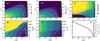 |
Fig. 4 Two dimensional structure of the reference disk model CI_XN. The height of the disk z is scaled by the radius (z/r). From top left to the bottom right: a) gas number density n⟨ H ⟩; b) dust density ρdust (note the dust settling); c) FUV radiation field χ in units of the ISM Draine field; d) gas temperature Tgas; e) dust temperature Tdust and f) the vertical hydrogen column density N⟨ H ⟩ ,ver versus radius. The white dashed contour lines in each contour plot correspond to the levels shown in the respective colorbar. The black (red) solid contour in panel c) indicate a vertical (radial) visual extinction equal to unity. |
2.4. Disk model
To model the disk we used the radiation thermo-chemical disk code PRODIMO (Woitke et al. 2009, 2016; Kamp et al. 2010; Thi et al. 2011). PRODIMO solves the wavelength dependent continuum radiative transfer which provides the disk dust temperature and the local radiation field. The gas temperature (the balance between heating and cooling) was determined consistently with the chemical abundances. The chemical network included 235 different species and 3143 chemical reactions (see Appendix B for more details).
We used a disk model representing the main properties of a disk around a typical T Tauri star. The stellar properties and the disk structure of this model are identical to the so-called reference model presented in Woitke et al. (2016). Here we only provide a brief overview of the disk model and refer the reader to Woitke et al. (2016) for details.
In Fig. 4 we show the gas number density, dust density, the local far-UV (FUV) radiation field, gas temperature, dust temperature and the vertical hydrogen column density for the reference model (model CI_XN, see Sect. 2.5 and Table 5). All relevant disk model parameters are given in Table 4.
Main fixed parameters of the disk model.
Based on the similarity solution for viscous accretion disks, we used an axisymmetric flared gas density structure with a Gaussian vertical profile and a powerlaw with a tapered outer edge for the radial column density profile (e.g. Lynden-Bell & Pringle 1974; Andrews et al. 2009). The vertical scale height as a function of radius is expressed by a simple powerlaw. The disk has a total mass of 0.01 M⊙ and extends from 0.07 au (the dust sublimation radius) to 620 au where the total vertical hydrogen column density reaches N⟨ H ⟩ ,ver ≈ 1020 cm-2 (panel (f) in Fig. 4).
For the dust density distribution we assumed a dust to gas mass ratio of d/g = 0.01. There is observational evidence for dust growth and settling in protoplanetary disks (e.g. Williams & Cieza 2011; Dullemond & Dominik 2004). To account for dust growth we assumed a power law dust size distribution f(a) = a-3.5 with a minimum and maximum grain radius of amin = 0.05 μm and amax = 3000 μm. For dust settling we applied the method of Dubrulle et al. (1995) with a turbulent mixing parameter of 10-2.
The irradiation of the disk by the star is important for the temperature and the chemical composition of the disk. For the photospheric emission of the star we use PHOENIX stellar atmosphere models (Brott & Hauschildt 2005). We considered a 0.7 M⊙ star with an effective temperature of 4000 K and a luminosity of 1L⊙. In addition to the photospheric emission, T Tauri stars commonly show far ultra-violet (FUV) excess (e.g. France et al. 2014) due to accretion shocks and strong X-ray emission (e.g. Güdel & Nazé 2009). For the excess FUV emission, we used a simple power law spectrum with a total integrated FUV luminosity of LFUV = 0.01 L∗, in the wavelength interval [91.2 nm, 250 nm]. The details for the stellar X-ray properties are discussed in Sect. 2.3.1 above.
We use the molecules HCO+ and N2H+ primarily to study the impact of SP ionization. To verify if our model gives reasonable results concerning HCO+ and N2H+ abundances, we compared the modelled fluxes for the J = 3 − 2 transition of HCO+ and N2H+ with the observational sample of Öberg et al. (2010, 2011a) finding a good agreement (for details see Appendix E).
2.5. Model series
It is likely that the different ionization sources are correlated. As already discussed the SP flux of young stars is actually derived from their stellar X-ray properties (Lee et al. 1998b; Feigelson et al. 2002). Also the CR ionization rate might be anti-correlated with the activity of the star (Cleeves et al. 2013). However, these possible correlations are not well understood. We therefore ran a series of full disk models using the X-ray, SP and CR spectra (described above) as inputs and also included the Turner SP model (Appendix D). We do not discuss any model with the active Sun SP spectrum as in this case SPs do not have a significant impact on the disk chemical structure (see Sect. 3.1). An overview of all presented models is given in Table 5.
Model series.
3. Results
3.1. Ionization rates as a function of column density
Before we discuss our results for the full disk model, we compare the SP, X-ray and CR ionization rates as a function of the total hydrogen column density N⟨ H ⟩ (N⟨ H ⟩ = NH + 2NH2). Figure 5 shows such a comparison for our different input spectra discussed in Sects. 2.2 and 2.3.
From visual inspection of Fig. 5 it becomes clear that for a SP flux comparable to our Sun (active Sun spectrum) SP ionization cannot compete with X-ray ionization assuming typical T Tauri X-ray luminosities. However, for the active T Tauri SP spectrum SP ionization becomes comparable to X-ray ionization or even dominates for N⟨ H ⟩ ≲ 1024 − 1025 cm-2. For NH ≲ 1023 cm-2ζSP is determined by the particles with Ep ≲ 5 × 10⁷ eV whereas higher energy particles dominate for N⟨ H ⟩ ≳ 1023 cm-2. The kink at N⟨ H ⟩ ≈ 2 × 1025 cm-2 is caused by the rapid attenuation of the SPs at high column densities. At such high column densities even the most energetic particles have lost most of their energy and the ionization rate drops exponentially.
For X-rays, Fig. 5 shows the differences between the normal and high X-ray spectrum. The X-ray ionization rates are higher for the high X-ray spectrum due to the higher X-ray luminosity. Additionally, the harder X-ray photons can penetrate to deeper layers but are also more efficiently scattered than lower energy X-ray photons. Compared to the normal X-ray case, the X-ray ionization rate increases by several orders of magnitude for N⟨ H ⟩ ≳ 1024 cm-2 for the high X-ray case.
Galactic cosmic rays are the most energetic ionization source. The peak in the particle energy distribution is around 108 − 109 eV (see Fig. 2). As a consequence the CR ionization rate ζCR stays mostly constant and only decrease for N⟨ H ⟩ ≳ 1025 cm-2. Only for such high column densities CR particle absorption becomes efficient.
In the Turner model it is implicitly assumed that SPs have the same energy distribution than Galactic CRs (see Appendix D). As a consequence the SP ionization rate in the Turner model is simply a scaled up version of the CR ionization rate. The slight differences to our model in CR attenuation is caused by the different methods used to calculate the SP/CR ionization rates; Turner & Drake (2009) use the fitting formulae of Umebayashi & Nakano (2009). Compared to our active T Tauri SP spectrum ζSP in the Turner model is larger for N⟨ H ⟩> 1025 cm-2 but significantly lower at low column densities.
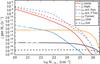 |
Fig. 5 SP, CR and X-ray ionization rates ζ as a function of hydrogen column density N⟨ H ⟩. |
3.2. Disk ionization rates
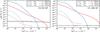 |
Fig. 6 Ionization rates ζ as a function of vertical column density N⟨ H ⟩ ,ver at radii of 1 and 100 au (solid and dashed lines respectively). The maximum values for N⟨ H ⟩ ,ver at the midplane of the disk, are N⟨ H ⟩ ,ver ≈ 4 × 1025 cm-2 and N⟨ H ⟩ ,ver ≈ 2 × 1023 cm-2 at 1 au and 100 au, respectively. Red lines are for X-rays, blue lines are for SPs and the black lines are for CRs. Left panel: model CI_XN_SP with ISM CRs and normal X-rays; right panel: model CL_XH_SP with low CRs and high X-rays. |
In Fig. 6 we show the ionization rates as a function of the vertical hydrogen column density N⟨ H ⟩ ,ver at two different radii of the disk. Shown on the figure are the models CI_XN_SP (ISM CR, normal X-rays; left panel) and CL_XH_SP (low CR, high X-rays; right panel).
CRs are only significantly attenuated for N⟨ H ⟩ ,ver> 1025 cm-2 and r ≲ 1 au. For most of the disk, CRs provide a nearly constant ionization rate of ζCR ≈ 2 × 10-17 s-1 for the ISM like and ζCR ≈ 2 × 10-19 s-1 for the low CR spectrum.
X-rays are strongly attenuated as a function of height and radius (i.e. geometric dilution). However, due to scattering X-rays can become the dominant midplane ionization source for large regions of the disk. For ISM-like CRs, CR ionization is the dominant midplane ionization source even in the high X-ray models. In the low CRs models X-rays are the dominant midplane ionization source for r ≲ 100 au in the normal X-ray model and for all radii in the high X-ray model.
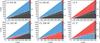 |
Fig. 7 Dominant disk ionization source throughout the disk. A light grey area indicates a region without a dominant ionization source. The different possible ionization sources, X-rays, SPs and CRs are identified by the different colors (color bar). The white solid contour line shows N⟨ H ⟩ ,rad = 1025 cm-2 the white dashed line shows the CO ice line. The model names are given in the top left of each panel. Top row: models with ISM CR ionization rate (CI); bottom row: models with low CR ionization rate (CL). First column: normal X-ray models (XN); second column: high X-ray models (XH); third column: turner models (T). |
Differently to X-rays, SPs are not scattered towards the midplane. Due to their high energies they propagate along straight lines (provided that the SPs are not shielded by magnetic fields, see Sect. 4.3.2). As SPs are of stellar origin they penetrate the disk only along radial rays. The radial column densities close to the midplane of the disk are N⟨ H ⟩ ,rad ≫ 1025 cm-2 and therefore SPs are already strongly attenuated at the inner rim of the disk. From Fig. 6 we see that the SP ionization rate ζSP drops below 10-19 s-1 for N⟨ H ⟩ ,ver ≳ 1024 cm-2 at r = 1 au and for N⟨ H ⟩ ,ver ≳ 1022 cm-2 at r = 100 au. However, at higher layers (N⟨ H ⟩ ,ver ≲ 1022 − 1023 cm-2) SPs are the dominant ionization source even in the high X-ray models. Expressed in radial column densities: SPs are the dominant ionization source in disk regions with N⟨ H ⟩ ,rad ≲ 1024 − 1025 cm-2.
In Fig. 7 we show the dominant ionization source at every point in the disk for all SP models. An ionization source is dominant at a certain point in the disk if its value is higher than the sum of the two other ionization sources. The first two columns in Fig. 7 show our models, the last column shows the Turner models. In our models, SPs are the dominant ionization source in the upper layers of the disk (above the white solid contour line for N⟨ H ⟩ ,rad = 1025 cm-2), whereas in the midplane always CRs or X-rays dominate.
For the Turner model the picture is quite different. In their model SPs can also penetrate the disk vertically (Appendix D) and reach higher vertical column densities before they are completely attenuated (Fig. 5). As a consequence SPs can become the dominant ionization source in the midplane of the disk (e.g. for the low CR case). In the upper layers always X-rays dominate as ζSP<ζX for low column densities. In the Turner model ζSP ≲ 10-13 s-1 for N⟨ H ⟩ ,rad< 1025 cm-2 which is several orders of magnitudes lower than in our models. The reason for this is that in the Turner model SPs are simply a scaled version of ISM like CRs. The high ζSP values in our model in the upper layers of the disk are caused by the high number of particles with energies Ep ≲ 108 eV, which are missing in the Turner model.
3.3. Impact on HCO+ and N2H+
The molecules HCO+ and N2H+ are the two most observed molecular ions in disks (e.g. Dutrey et al. 2014) and are commonly used to trace the ionization structure of disks (e.g. Dutrey et al. 2007; Öberg et al. 2011b; Cleeves et al. 2015). Also Ceccarelli et al. (2014) used these two molecules to trace SPs in a protostellar envelope.
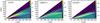 |
Fig. 8 Abundances ϵ(X) relative to hydrogen for CO, HCO+ and N2H+ for the reference model CI_XN. The white solid contour line shows N⟨ H ⟩ ,rad = 1025 cm-2, the white dashed line shows the CO ice line. We call the regions above and below the CO ice line the warm and cold molecular layer, respectively. The dotted iso-contours show where the X-ray ionization rate is equal to the ISM CR (ζCR = 2 × 10-17 s-1) and equal to the low CR (ζCR = 2 × 10-19 s-1) ionization rate, respectively. |
The main formation path of HCO+ and N2H+ is the ion-neutral reaction of H with their parent molecules CO and N2, respectively. H is created by ionization of H2 by CRs, X-rays and in our model additionally by SPs. The main destruction pathway for HCO+ and N2H+ is via dissociative recombination with free electrons.
The chemistry of HCO+ and N2H+ is linked to the CO freeze-out. To form HCO+, gas phase CO is required, whereas N2H+ is efficiently destroyed by CO (e.g. Aikawa et al. 2015). Consequently the N2H+ abundance peaks in regions where CO is depleted and N2, the precursor of N2H+, is still in the gas phase. The result of this chemical interaction is a vertically layered chemical structure for HCO+ and N2H+ (see Fig. 8). For further details on the HCO+ and N2H+ chemistry see Appendix B, where we also list the main formation and destruction pathways for HCO+ and N2H+ (Table B.1).
3.3.1. Abundance structure
In the following we describe details of the molecular abundance structure that are relevant for the presentation of our results for our reference model CI_XN. The abundance ϵ of a molecule X is given by ϵ(X) = nX/n⟨ H ⟩, where nX is the number density of the respective molecule and n⟨ H ⟩ = nH + 2 nH2 is the total hydrogen number density. Figure 8 shows the resulting abundance structure for CO, HCO+ and N2H+ for the CI_XN model.
We define the location of the CO ice line where the CO gas phase abundance is equal to the CO ice-phase abundance (white dashed line in Fig. 8). The CO ice line is located at dust temperatures in the range Td ≈ 23 − 32 K (density dependence of the adsorption/desorption equilibrium; e.g. Furuya & Aikawa 2014). The radial CO ice line in the midplane (z = 0 au) is at r ≈ 12 au and Td ≈ 32 K. At r ≈ 50 au the vertical CO ice line is at z ≈ 8.5 au (z/r ≈ 0.17) and Td ≈ 26 K. Inside/above the CO ice line ϵ(CO) ≈ 10-4. Outside/below the CO ice line ϵ(CO) rapidly drops to values ≲10-6. In regions where non-thermal desorption processes are efficient (r ≳ 150 au) ϵ(CO) ≈ 10-6 down to the midplane. For the regions inside/above and outside/below the CO ice line we use the terms warm and cold molecular layer, respectively.
There are two main reservoirs for HCO+, one in the warm molecular layer above the CO ice line and one in the outer disk (r ≳ 150 au) below the CO ice line where non-thermal desorption becomes efficient. In the warm molecular layer, the ionization fraction ϵ(e−) ≈ 10-7 is dominated by sulphur as it is ionized by UV radiation (e.g. Teague et al. 2015, see also Sect. 4.2.3). Those free electrons efficiently destroy molecular ions via dissociative recombination. This causes a dip in the vertical HCO+ abundance structure within the warm molecular layer with ϵ(HCO+) ≈ 10-12 − 10-11, whereas at the top and the bottom of the warm molecular layer ϵ(HCO+) reaches values of ≈10-10 − 10-9. The peak in the top layer is mainly caused by the high X-ray ionization rate for H2 (ζX ≳ 10-12 s-1). At the bottom of the warm molecular layer more HCO+ survives. This region is already sufficiently shielded from UV radiation and the free electron abundance drops rapidly. In the second reservoir, below the CO ice line where non-thermal desorption is efficient ϵ(HCO+) ≈ 10-11 − 10-10.
The main N2H+ reservoir resides in the cold molecular layer just below the CO ice line with ϵ(N2H+) ≳ 10-11. The lower boundary of this layer with ϵ(N2H+) < 10-11 is reached at Td ≈ 16 K where ϵ(N2) ≲ 10-6 due to freeze-out. Radially this layer extends from the inner midplane CO ice line out to r ≈ 250 − 300 au. Close to the midplane ϵ(N2H+) ≲ 10-12 for r ≳ 150 au due to non-thermal desorption of ices. There is also a thin N2H+ layer at the top of the warm molecular layer with ϵ(N2H+) ≈ 10-12 extending from the inner radius of the disk out to r ≈ 100 au. In this layer the X-ray ionization rate is high enough to compensate for the destruction of N2H+ by CO.
The detailed appearance of this layered structure is especially sensitive to the dust temperature and therefore also to dust properties (e.g. dust size distribution). The above described abundance structure for CO, HCO+ and N2H+ is consistent with the model of Aikawa et al. (2015) that includes millimetre sized dust particles with a dust size distribution similar to what is used here (for details see Appendix B).
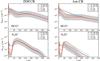 |
Fig. 9 Vertical column density profiles for HCO+ and N2H+ for our model series (Table 5). The left column shows the models with the ISM like CRs (ζCR ≈ 2 × 10-17 s-1), the right column with low CRs (ζCR ≈ 2 × 10-19 s-1). The top row shows HCO+, the bottom row N2H+. The blue lines are for models with, the red lines are for models without SPs. Dashed (solid) lines are for models with high (normal) X-rays. The orange solid line shows the Turner model. The grey shaded area marks a difference of a factor 3 in the column densities relative to the CI_XN (ISM CR, normal X-rays) and CL_XN model (low CR, normal X-rays), respectively. |
3.3.2. Vertical column densities
To study the impact of SP ionization quantitatively we compare vertical column densities of HCO+ and N2H+ for models with and without SPs. In Fig. 9 we show the vertical column densities NHCO+ and NN2H+ as a function of the disk radius r for all models listed in Table 5. The left column in Fig. 9 shows the models with ISM CRs, the right column the models with low CRs. At first we discuss the models without SPs and compare them to other theoretical models.
The NHCO+ profile shows a dip around r ≈ 50 − 100 au in the ISM CR models CI_XN and CI_XH (high X-rays). This dip is also seen in the models of Cleeves et al. (2014). Unlike Cleeves et al. (2014), in our model this dip is not predominantly due to the erosion of CO by reactions with He+ (“sink effect” e.g. Aikawa et al. 1997, 2015; Bergin et al. 2014; Furuya & Aikawa 2014), but mainly due to the interplay of CO freeze-out and non-thermal desorption in the outer disk. The CO sink effect is also active in our model but less efficient (see Appendix B.2.2).
The lack of HCO+ in the disk midplane at r ≈ 50 − 100 au due to CO freeze-out is also visible in the HCO+ abundance structure shown in Fig. 8. Non-thermal desorption in the midplane produces CO abundances ≳10-7 for r ≳ 150 au and consequently also a slight increase in NHCO+. In the low CR models the ionization rate is too low to produce a significant amount of HCO+ in the cold molecular layer and the dip in the profile vanishes.
N2H+ traces the distribution of gas phase CO as it is efficiently destroyed by CO (Qi et al. 2013a,b, 2015). This is also seen in our model. The sharp transition in the N2H+ column density at r ≈ 30 au traces the onset of CO freeze-out (Fig. 9). We note, however, that the actual midplane CO ice-line is at ≈ 12 au (see Appendix C for details). In the ISM CR models NN2H+ is dominated by CR ionization as N2H+ mainly resides in the cold molecular layer. In the warm N2H+ layer X-ray ionization dominates. However, due to the lower densities in the warm molecular layer, this layer only contributes significantly to the column density within the radial CO ice line, and the impact of X-rays is only visible there (compare models CI_XH and CI_XN in Fig. 9). The high X-ray luminosity decreases the contrast between the peak of NN2H+ close to the radial CO ice line and NN2H+ inside the CO ice line by about a factor of five.
For the low CR case NN2H+ drops by more than an order of magnitude compared to the ISM CR case. Such a strong impact of CR ionization on NN2H+ is also reported by Aikawa et al. (2015) and Cleeves et al. (2014). Higher X-ray luminosities can compensate for low CR ionization only to some extent. In the high X-ray model CL_XH, NN2H + is lower by a factor of five compared to the ISM CR models.
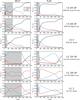 |
Fig. 10 Ionization rate weighted column densities Nζ (Eq. (5)) as a function of radius for HCO+ (left column) and N2H+ (right column). Nζ is normalized to the total column density of the respective molecule. The individual colored solid lines show the fraction of the total column density dominated by a certain ionization source. Red is for X-rays (NζX), blue for SPs (NζSP) and black for CRs (NζCR). Each row corresponds to one model. On the right hand side the model descriptions are provided (see Table 5). The grey shaded area marks the region where more than 50% of the column density arise from regions above the CO ice line (i.e. the warm molecular layer). |
3.3.3. Impact of SPs
The column densities NHCO+ and NN2H+ for models with SPs are shown in Fig. 9 (blue solid and dashed lines). The solid orange line in Fig. 9 shows the results for the Turner model. We discuss the Turner model separately in Sect. 3.3.4. We define a change in the column densities by at least a factor of three compared to the reference model as significant. This is indicated by the grey area around the column density profiles of the reference models CI_XN and CL_XN.
To better quantify the impact of SPs compared to the competing H2 ionization sources , X-rays and CRs, we introduce the weighted column density ![Mathematical equation: \begin{equation} \label{eqn:nzeta} N_\mathrm{\zeta}(r)=\int^{\infty}_0 n(r,z)\times f_\zeta(r,z)\,\mathrm{d}z\,\,\mathrm{[cm^{-2}]}. \end{equation}](/articles/aa/full_html/2017/07/aa30241-16/aa30241-16-eq220.png) (5)Nζ is the weighted column density for a particular H2 ionization source ζ, n is the number density of a particular molecule in units of cm-3 and
(5)Nζ is the weighted column density for a particular H2 ionization source ζ, n is the number density of a particular molecule in units of cm-3 and 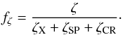 (6)Nζ represents the fraction of the column density dominated by a particular ionization source ζ.
In Fig. 10 we show Nζ for HCO+ and N2H+ normalized to the total column density of the respective molecule as a function of radius. The region where more than 50% of the total column density of the molecules arise from disk regions above the CO ice line (i.e. from the warm molecular layer) is roughly indicated on each plot.
SP ionization has a significant impact on the NHCO+ profile in all our models. In the ISM CR model (CI_XN_SP) NHCO+ increases by a factor ≈3 for 50 ≲ r ≲ 100 au and the dip in the profile seen in the models without SPs (CI_XN) vanishes (top left panel in Fig. 9). In the low CR models this region increases to 25 ≲ r ≲ 150 au and NHCO+ reaches values up to an order of magnitude higher compared to the CL_XN model (top right panel in Fig. 9). In the models with high X-rays, SP ionization still has an significant impact and NHCO+ increases by up to a factor of three (dashed lines in Fig. 9).
This situation is also clearly visible in Fig. 10 where we show Nζ as a function of radius (Eq. (5)). Although X-rays can be the dominant ionization source close to the star, in all models NHCO+ is dominated by SP ionization for 50 ≲ r ≲ 100 − 200 au. Figure 10 also shows that in the low CR models NHCO+ is mainly built up in the warm molecular layer for r ≲ 200 au. In this region (indicated in Fig. 10) the warm molecular layer contributes more to the total column density than the cold molecular layer.
For N2H+ the picture is more complex. In the ISM CR models SPs have only very little impact on NN2H+. Only in the inner 30 au, within the radial CO ice line, the N2H+ profile is significantly affected. The reason for this is the high SP ionization rate ζSP ≳ 10-12 s-1 in the warm molecular layer of the disk close to the star. In this region the abundance ratio of HCO+/N2H+ drops from >103, in the models without SPs, to around 10 to 100 in models with SPs. These high ratios can be explained by the efficient destruction of N2H+ by CO. However, due to the high ζSP this destruction path becomes less important, and the molecular ion abundance are mainly determined by the balance between ionization and recombination.
Ceccarelli et al. (2014) reported a very low measured HCO+/N2H+ ratio between three and four in the Class 0 source OMC-2 FIR 4. They explain this low ratio by the high ionization rates due to SPs (ζSP> 10-14). In our disk model ζSP in the warm molecular layer is comparable, but the HCO+/N2H+ ratio is much larger than four. This higher ratio is due to the higher densities of 108 − 1010 cm-3 and the stronger UV field in the warm molecular layer, compared to the physical conditions in OMC-2 FIR 4. This is in agreement with the chemical models presented in Ceccarelli et al. (2014).
The impact of SPs on the N2H+ abundance in the warm layer can extend out to r ≈ 200 au (similar to HCO+). However, for r> 30 au this layer does not significantly contribute to the total N2H+ column density as NN2H+ is dominated by the high density layer below the vertical CO ice line.
Beyond the radial CO ice line NN2H+ is dominated by CRs in the ISM CR models and is not affected by X-rays nor SPs (bottom left panel in Fig. 9). Compared to the ISM CR models, NN2H+ is reduced by a factor of a few around the peak and by more than an order of magnitude at larger radii in the low CR models. As a consequence the profile is also steeper. Although higher X-rays (CL_XH model) and also SPs can to some extent compensate low CR ionization rates, the NN2H+ profile is still steeper and NN2H+ is lower by a factor of between approximately two and six than in the ISM CR models for r ≳ 30 au.
From Fig. 10 we see that only in the CL_XN_SP model SPs dominate NN2H+ for r ≳ 70 au. Actually the importance of SPs increases with r in this model. In the CL_XN_SP model SPs are the dominant ionization source in regions with N⟨ H ⟩ ,rad ≲ 1025 cm-2. The N⟨ H ⟩ ,rad = 1025 cm-2 iso-contour is below the vertical CO ice line for r> 70 au and the layer between the CO ice line and N⟨ H ⟩ ,rad = 1025 cm-2 becomes thicker with radius (see Figs. 7 and 8). This also explains the change in the slope of NN2H+ compared to models without SPs.
In the high X-ray model, CL_XH_SP, the picture is quite different. NN2H+ is now dominated by X-rays for r ≳ 30 au. X-rays are efficiently scattered towards the midplane and therefore ζX>ζSP in the cold N2H+ layer (see also Fig. 7). X-rays affect the cold N2H+ layer at all radii therefore the slope of NN2H+ is steeper than in the model where SP dominate (compare the blue solid line with the red dashed line in Fig. 9).
Our results show that HCO+ is always significantly affected by SP ionization but N2H+ only in models with low CRs and normal X-rays (for r> 30 au). As SPs can only reach the upper layers of the cold molecular layer, N2H+ is less sensitive to SP ionization than HCO+.
3.3.4. Impact of SPs in the Turner model
In the Turner model SP ionization is just a scaled up version of CR ionization where SPs can also penetrate the disk vertically (see Appendix D). The results of the Turner models are also shown in Figs. 9 and 10.
In the ISM CR models there is no significant impact on HCO+ and N2H+ by SP ionization. ζSP is significantly lower at low column densities compared to our models (see Sect. 3.1). Therefore X-rays are the dominant ionization source in the warm molecular layer and HCO+ is not significantly affected by SP ionization. The slight increase in the HCO+ column density is mainly due to the higher X-ray luminosity in the Turner model compared to our reference model with normal X-rays. Similar to our models CRs dominate in the cold molecular layer.
In the Turner model with low CRs, SPs become the dominant ionization source in the cold molecular layer as they also penetrate the disk vertically. In this layer ζSP reaches values of ≈10-17 s-1 at r ≈ 100 au. However, in the Turner model SPs also cannot compensate for a low CR ionization rate as ζSP ∝ 1 /r2 (geometric dilution).
The impact of SPs in the Turner model is rather limited and restricted to the cold molecular layer, in strong contrast to our models. The differences are mainly due to the assumptions concerning the SP transport. In the Turner model SPs hit the surface of the disk and penetrate the disk vertically, whereas we assume that SPs travel only along radial rays. However, both approaches are an approximation of a likely more complex picture of SP transport in disks. We discuss this in more detail in Sect. 4.3.
4. Discussion
4.1. Constraining the SP flux of T Tauri stars
SP ionization has a significant impact on the column densities of HCO+ and N2H+ in all our models. To actually constrain the SP flux from observations it is necessary to disentangle the contribution of SP ionization from the competing ionization sources CRs and X-rays.
From a chemical point of view all three ionization sources act the same way, they ionize molecular hydrogen and drive the molecular ion chemistry. However, they also show distinct differences in how they irradiate and penetrate the disk. CRs act like a background source and irradiate the disk isotropically, whereas X-rays and SPs originate from the star and act like a point source. A further difference is their energy distribution. Because of their high energies, CRs and SPs tend to move on straight lines whereas (hard) X-rays also experience scattering during their interaction with the disk.
Those differences in their irradiation properties and their energy distribution allow to disentangle their impact on the ion chemistry at different locations in the disk. Our models show that the stellar ionization sources are more effective closer to the star and at the surface layers of the disk (Fig. 10). X-rays can also become an important ionization source in the midplane of the disk but not for the whole disk as, roughly speaking, the ionization rate of stellar ionization sources is ∝1 /r2. CR ionization affects the whole disk, but is, in contrast to the stellar ionization sources, more important for the outer disk and the cold layers and the midplane of the disk (this argument also holds for SLR ionization).
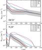 |
Fig. 11 Comparison of column densities for HCO+ (top) and N2H+ (bottom) for models with varying SP flux and very strong X-ray emission. For all models the low CR ionization rates are used. Shown are the reference model with normal X-rays (black, CL_XN), the model with the typical SP flux (blue, CL_XN_SP) and models with a factor of ten higher (purple, CL_XN_SPH) and factor of ten lower (red, CL_XN_SPL) SP flux. The dashed black line shows the model with LX = 3 × 1031 erg s-1 and no SPs. The grey shaded area marks a difference of a factor of three in the column densities relative to the reference model CL_XN. |
So far we have only shown models using the commonly proposed SP flux of fp(Ep ≥ 10 MeV) ≈ 107 protons cm-2 s-1 (e.g. Feigelson et al. 2002). However, this value should be only seen as an order of magnitude estimate (see Sect. 2.2).
In Fig. 11 we show the column densities for HCO+ and N2H+ for models with a SP flux a factor of ten higher and lower with respect to the reference value. Also shown are the reference model for the low CR case CL_XN and the model with the reference SP flux CL_XN_SP. For these models we use the low CR ionization rate (ζCR ≈ 2 × 10-19 s-1) and the normal X-ray luminosity (LX = 1030 erg s-1). Further we show a model with LX = 3 × 1031 erg s-1, to illustrated the impact of (very) strong X-ray emission (e.g. ζX ≳ 10-17 s-1 in the disk midplane).
In the low SP flux model (CL_XN_SPL) the impact on HCO+ and N2H+ is quite limited. For such a case it is still possible to define upper limits for the SP flux in disks.
In the high SP flux model (CL_XN_SPH) the SP ionization rate reaches values of ζSP ≳ 10-13 s-1 and ζSP ≈ 10-17 s-1 in the warm and cold molecular layer respectively. The N2H+ column density profile beyond the radial CO ice line is comparable to the profile for models with ISM CRs (compare with Fig. 9). Also the model with very high X-rays (CL_X31) and no SPs shows a similar profile for N2H+. However, as seen from Fig. 11 the corresponding HCO+ profiles differ significantly.
Comparing the very high X-ray model (CL_X31) to the reference model with SPs (CL_XN_SP) shows that the corresponding HCO+ profiles are similar but the N2H+ profiles differ by an order of magnitude. This shows again that it is indeed possible to distinguish between the different ionization sources by simultaneous modelling of HCO+ and N2H+ column density profiles.
To trace this interplay of ionization sources, spatially resolved observations of molecular ion lines tracing different vertical layers of the disk are required. With modern (sub)millimetre interferometers like the Atacama Large Millimeter Array (ALMA), the NOrthern Extended Millimeter Array (NOEMA) and the Submillimeter Array (SMA) such observations with a spatial resolution of tens of au are already possible (e.g. Qi et al. 2013b; Cleeves et al. 2015; ALMA Partnership et al. 2015; Yen et al. 2016) and will become available on a regular basis in the near future. Here, we use HCO+ and N2H+ as the tracers of the warm and cold molecular layer respectively, but also other molecules like DCO+, which traces similar regions as N2H+ (Teague et al. 2015; Mathews et al. 2013) can be used.
Complementary, far-infrared lines of HCO+ and N2H+, as used by Ceccarelli et al. (2014) to trace SP ionization in a protostellar envelope, are good tracers of molecular ion emission in the warm inner region of the disk. However, a more detailed analysis with proper modelling of line emission is required to identify the best observational tracers of SP ionization. We will present such an analysis in a follow-up paper.
4.2. Chemical implications
Besides the H2 ionization rates there are other “chemical parameters”, which have an impact on the molecular ion abundance in disks. In the following we discuss the dependence of our results on the location of the CO ice line, depletion of CO and the assumed initial metal abundances. Those chemical properties of disks are not well constrained from observations and/or can vary between different targets.
4.2.1. Location of the CO ice line
Recent ALMA observations provide direct constrains on the location of the CO ice line. However, these results depend on the method or more precisely the molecule used to trace the CO ice line (see Qi et al. 2013b; Schwarz et al. 2016; Nomura et al. 2016, for TW Hya). Further, due to complex chemical processes like the CO sink effect it is possible that the actual location of the CO ice line does not only depend on the CO freeze-out temperature (Aikawa et al. 2015, Sect. 3.3.2).
To investigate the dependence of our results on the location of the CO ice line we artificially moved the CO ice line in our model by adapting the binding energy for CO. We consider two cases: EB(CO) = 950 K and EB(CO) = 1350 K (i.e 200 K lower and higher compared to our reference model). In both cases we kept the ratio of EB(N2) /EB(CO) = 0.67 constant (see Appendix B.2.2). As a consequence also the N2H+ layer moves accordingly to the CO ice line (see Sect. 3.3.1). For EB(CO) = 950 K the CO ice line moves to Td ≈ 20 − 24 K, (i.e. deeper into the disk) and for EB(CO) = 1350 K to Td ≈ 25 − 36 K (i.e. higher up in the disk).
For a CO ice line deeper in the disk the contribution of CR ionization to the total column of HCO+ and N2H+ increases in the ISM CR models. In the ISM CR models SP ionization is not significant anymore (i.e. NHCO+ increases by less than a factor two). However, in the low CR models the impact of SPs remains significant.
A CO ice line higher up in the disk has the opposite effect. The total column densities of the molecular ions are now dominated by layers higher up in the disk which can efficiently be ionized by SPs. As a consequence the relative contribution of SP ionization to NHCO+ and NN2H+ increases.
In summary for a CO ice line location deeper in the disk SP ionization becomes less important, for a CO ice line higher up in the disk SP ionization becomes more important. However, in both cases the interplay of the different ionization sources is qualitatively speaking similar to what is shown in Fig. 10.
4.2.2. CO depletion
There is observational evidence for CO depletion in protoplanetary disks (Dutrey et al. 1997; Bruderer et al. 2012; Favre et al. 2013; Kama et al. 2016a; Schwarz et al. 2016; McClure et al. 2016). The best constraint case is TW Hya. Using spatially resolved ALMA spectral line observations of several CO isotopologues Schwarz et al. (2016) derived a uniform CO abundance of ≈10-6 in the warm molecular layer, two order of magnitudes lower than the canonical value of ≈10-4. However, the degree of CO depletion seems to vary from source to source. Using Herschel HD J = 1 − 0 line observations McClure et al. (2016) derived CO depletions of a factor of approximately five and up to ≈100 for DM Tau and GM Aur, respectively.
The cause of CO depletion in disks is not yet clear. Although freeze-out of CO certainly contributes to depletion it is unlikely that it is the only process acting. Several other mechanisms that can at least partly explain CO depletion are proposed:
-
the destruction of CO by He+ and the subsequent conversion of atomic carbon to more complex carbon bearing molecules with higher freeze-out temperatures (Aikawa et al. 1996; Bergin et al. 2014; Helling et al. 2014; Furuya & Aikawa 2014);
-
depletion of CO in layers above the CO ice line (up to T ≈ 30 K) due to conversion of CO to CO2 on the surfaces of dust grains (Reboussin et al. 2015);
-
CO isotopologue selective photodissociation, which affects CO isotopologue line emission and therefore the derived CO depletion factors;
-
carbon and/or oxygen depletion in the warm disk atmosphere due to settling and mixing of ice coated dust grains (Du et al. 2015; Kama et al. 2016b).
It is as yet unclear which of the proposed mechanisms is the most efficient one; none of them can be excluded with certainty. It is also possible that all of these processes are at work. So far the impact of CO (carbon and/or oxygen depletion) on molecular ion emission was not studied in detail. For the modelling of HCO+ and N2H+ line emission of TW Hya, Cleeves et al. (2015) reduced the initial atomic carbon abundance by two orders of magnitude to match C18O line observation. However, the impact of C and CO depletion on HCO+ and N2H+ was not discussed in detail.
To simulate CO depletion we simply reduce the total carbon and oxygen element abundances by one order of magnitude throughout the disk. This results in a CO abundance of ≈10-5 in the warm molecular layer. We applied this “artificial” CO depletion to all models listed in Table 5; all other parameters of the models are fixed.
The CO depletion models show a factor of ≈5 − 10 lower NHCO+ for r ≳ 50 au compared to the non depleted models. For r< 30 auNN2H+ increases by more than an order of magnitude. NN2H+ beyond the CO ice line is not affected as NN2H+ resides within the CO freeze-out zone where gas phase CO is anyway depleted.
In the CO depletion models SP ionization is slightly more efficient for NN2H+ as the contribution of the warm N2H+ layer to NN2H+ increases. Due to the lower CO abundance in the warm molecular layer the N2H+ abundance increases as the destruction pathway via CO is less efficient. For HCO+ the opposite is true. The HCO+ abundance decreases by roughly an order of magnitude in the warm molecular layer, whereas in the CO freeze-out zone the impact is smaller (i.e. CO is frozen-out anyway). Relatively speaking the contribution of the cold HCO+ to NHCO+ increases in the CO depletion models. Therefore the impact of SPs on NHCO+ is less significant whereas X-rays and CRs become more important. Although there are some differences, the impact of SPs on NN2H+ and NHCO+ is qualitatively very similar to the non-depleted models. In particular the main trends derived from Fig. 10 are also seen in the CO depletion models.
CO depletion is certainly more complex than modelled here. A more thorough study of the impact of CO depletion on molecular ion abundances is certainly desirable and possibly provides new constraints on CO gas phase depletion in disks. However, this is beyond the scope of this paper.
4.2.3. Metal abundances
Heavy metals such as sulphur play an important role in the molecular ion disk chemistry (Teague et al. 2015, Rab et al., in prep.). Here we refer with the term metals to the elements Na, Mg, Si, S and Fe. Metal ionization due to UV radiation can produce a large number of free electrons. Those free electrons destroy molecular ions like HCO+ and N2H+ via dissociative recombination. Dissociative recombination is more efficient than radiative recombination of metals. As a consequence a high abundance of metals significantly reduces the abundance of molecular ions (e.g. Mitchell et al. 1978; Graedel et al. 1982).
In the ISM and in disks most of the metals are likely locked up in refractory grains and are therefore depleted compared to Solar abundances. We use metal abundances similar to the commonly used “low metal” abundances (Graedel et al. 1982; Lee et al. 1998a). These low metal abundances are depleted by a factor of ≈100 − 1000 compared to Solar abundances (i.e. low metal sulphur abundance ϵ(S) ≈ 10-7). However, the actual gas phase abundance of metals is difficult to constrain from observations and a stronger degree of depletion already prior to disk formation is possible (e.g. Maret & Bergin 2007; Maret et al. 2013).
To investigate the dependence of our results on the metal abundances we deplete the initial gas phase metal abundance by an additional factor of ten compared to the low metal abundances (i.e. ϵ(S) ≈ 10-8). This means that a larger fraction of metals is locked-up in refractory dust grains and cannot be released back into the gas phase.
Decreasing the metal abundances increases ϵ(HCO+) in the warm molecular layer by up to an order of magnitude (i.e. the gap in the vertical ϵ(HCO+) profile nearly vanishes; Sect. 3.3.1). In the cold molecular layer the metal abundances are not as important since the metals are frozen-out on dust grains anyway. However, in regions where non-thermal desorption processes are efficient (i.e. metal ices are released back into the gas-phase), ϵ(HCO+) but also ϵ(N2H+) are higher by a factor of a few in the lower metal abundance models. The HCO+ column density is higher by a factor of between approximately two and three at all radii in the strong metal depletion models compared to the models with the reference abundances. The N2H+ column density is only affected for r ≳ 150 au (higher by a factor of between approximately two and three), where non-thermal desorption of metals is efficient.
Lower gas phase metal abundances lead to an increase of the molecular ion abundances in the warm molecular layer and the contribution of this layer to the total column densities increases. However, in the strong metal depletion models the interplay and the relative contributions to the column densities of the different ionization sources is nearly identical to the reference model grid (i.e. Fig. 10 does not change significantly). Our arguments concerning the impact of SPs on HCO+ and N2H+ are therefore also valid for the case of strong metal depletion.
4.3. Future prospects
Our model results show that SPs can indeed become an important ionization source in T Tauri disks. However, our model should be seen as a first attempt at a comprehensive modelling of SP ionization in protoplanetary disks. In the following we discuss further important aspects like variability, non-stellar origin of SPs, the importance of magnetic fields and future prospects for SP modelling in protoplanetary disks.
4.3.1. Flares and variability
In our models we assumed continuous (i.e. time-averaged) particle fluxes and X-ray luminosities. Although this is a reasonable assumption (see Sect. 2.2) it is likely that the disk is also hit by singular powerful X-ray and/or SP flares.
From the X-ray COUP survey of the ONC cloud, Feigelson et al. (2002) and Wolk et al. (2005) derived a median X-ray flare luminosity of ≈6 × 1030 erg s-1, comparable to the X-ray luminosity in our high X-ray models, and peak flare luminosities up to 1031 erg s-1 . The duration of such flares can last from hours up to three days with a typical frequency of roughly one powerful flare per week.
Ilgner & Nelson (2006) argue that for such flare properties the disk ion chemistry responds to time-averaged ionization rates. However, in case the duration between two flares is longer than the recombination time scale in the disk, such singular and strong flares would produce asymmetric features in molecular ion emission (i.e. a singular flare only affects a certain fraction of the disk). The spatially resolved HCO+J = 3 − 2 SMA observations of TW Hya show indeed such an asymmetric structure (Cleeves et al. 2015). However, as discussed by Cleeves et al. (2015) these features could also have a different origin like spiral arms or an hidden planet locally heating the disk.
If such asymmetric structures are caused by stellar flares they would provide complementary constraints on the X-ray/SP activity of the star. Multi-epoch data of spatially resolved molecular ion emission is required to prove the flare scenario (i.e. the features should disappear quickly). The current (sub)mm interferometers like ALMA, NOEMA and SMA provide the required spatial resolution and might even allow for monitoring of disks in molecular ion lines on a daily/weekly basis in the future.
Modelling of such observations does not necessarily require 3D chemical models. Assuming that the disk physical structure is not affected by flares, radial cuts through the disk can be modelled with 2D (time-dependent) thermo-chemical models as presented here.
4.3.2. Magnetic fields
In our model we neglect the impact of magnetic fields on the SP transport. Stellar and disk magnetic fields are in particular relevant for the question if particles actually hit the disk (see Feigelson et al. 2002, for a discussion).
Magnetic fields can either drag the particles away from the disk (e.g. like in a wind) but could also funnel the particles and concentrate the ionizing flux in particular regions of the disk. In the first scenario SPs can still have an impact on the upper layers of the disk but certainly not on the disk midplane. In the second scenario particles are likely focused on regions close to the inner radius of the disk and their impact on the outer disk will become less significant. Also the trajectory of the particles will be affected, and they might penetrate the disk also vertically. Our models, where particles are transported only radially, are closer to the wind scenario whereas the Turner model would represent an extreme case for magnetically focused particles. However, to qualitatively estimate the impact of magnetic fields more complex SP transport models are required.
It is possible to consider magnetic field effects in high energy particle transport models (Desch et al. 2004; Padovani & Galli 2011; Padovani et al. 2013b). In principle such methods can also be applied to disk models. The main challenge though is to determine the structure of the star and disk magnetic fields. However, as argued by Ceccarelli et al. (2014) identifying distinct observational signatures of SP ionization in disks and/or envelopes would allow to derive constrains for the magnetic field structure. This is certainly challenging, but with the availability of spatially resolved observational data and interpretation of such data with (improved) thermo-chemical disk models this might be feasible in the near future.
4.3.3. Non-stellar origin of high energy particles
Besides the stellar surface the close environment of young stars offers also alternative particle acceleration sites. X-ray flares and particles can be produced close to the inner disk in the so called reconnection ring where the stellar and disk magnetic field interact (X-wind model Shu et al. 1994, 1997). More recently Padovani et al. (2015, 2016) proposed jet shocks as alternative acceleration sites for high energy particles.
In the X-wind model the particle source and also the X-ray emitting source is located closer to the disk and slightly above the disk midplane. The typically assumed source location in this “lamppost” scenario is rL ≈ 0.05 au and zL ≈ 0.05 au (≈10 R⊙) (Lee et al. 1998b; Igea & Glassgold 1999). For X-rays Ercolano et al. (2009) found that the height of the emitting source has relatively little impact concerning X-ray radiative transfer in disks. Moving the emitting source closer to the disk certainly has an impact on the very inner disk but for e.g. 10 au distance from the star the stellar particle flux increases only by about 1% compared to the stellar origin. The height of the SP emitting source has some impact on where in the disk SPs see a column density N⟨ H ⟩ ≳ 1025 cm-2. For particles accelerated at a height zL ≈ 0.05 au and moving along a ray parallel to the midplane this happens at r ≈ 0.5 au. The consequences are that SPs can penetrate into slightly deeper layers of the disks but they still cannot penetrate to the disk midplane. Therefore our conclusions on the impact of SPs on HCO+ and N2H+ remain valid for the X-wind scenario.
In the jet shock scenario, the emitting source would be located far above the disk. Padovani et al. (2016) considered a particle emitting source located at 1.8 × 10³ au above the star and calculated the resulting ionization rates for a 2D disk structure. Depending on their particle acceleration model they found ionization rates up to ζ ≈ 10-14 s-1 at the surface layers of the disk. Although X-ray ionization rates in the upper layer of the disk are typically higher such an irradiation scenario could have a significant impact on the ionization of the outer disk (r ≳ 50 au). In the outer disk, the jet accelerated particles can penetrate the disk vertically and therefore can also reach the disk midplane (similar to the Turner model, Sect. 3.3.4). This might become important if Galactic CRs are efficiently attenuated (i.e. in the low CR case).
The scenarios described above for non-stellar particle sources are certainly worth being investigated in detail. For the future we plan to extend our model to a proper treatment of such non-stellar emitting sources.
5. Summary and conclusions
In this work we investigated the impact of stellar energetic particle (SP) ionization on disk chemistry with a focus on the common disk ionization tracers HCO+ and N2H+. We assumed a typical SP flux of fp(Ep ≈ 10 MeV) ≈ 107 protons cm-2 s-1 (at 1 au) as commonly proposed for T Tauri stars and a particle energy distribution derived from measurements of solar particle events. Based on a detailed particle transport model we derived an easy to use formula (see Sect. 2.2) to calculate the SP ionization rate in the disk as a function of hydrogen column density and radius, assuming that the particles can penetrate the disk only radially. With a small grid of models considering varying properties of the competing high energy disk ionization sources, X-rays and Galactic cosmic rays, we studied the interplay of the different ionization sources and identified possible observational tracers of SP ionization. Our main conclusions are the following:
-
SPs cannot penetrate the disk mid-plane. At hydrogen column densitiesN⟨ H ⟩ ≳ 1025 cm-2 even the most energetic particles are attenuated (stopped) and the SP ionization rate drops rapidly. As the radial hydrogen column densities for full T Tauri disks are typically N⟨ H ⟩ ≫ 1025 cm-2 the midplane SP ionization rate is ζSP ≪ 10-20 s-1 already at a distance of 1 au from the star.
-
For the assumed SP flux (see above), SPs become the dominant H2 ionization source in the warm molecular layer of the disk above the CO ice line, provided that SPs are not shielded by magnetic fields. This is even true for enhanced X-ray luminosities (i.e. LX = 5 × 1030 erg s-1).
-
SP ionization can increase the HCO+ and N2H+ column densities by factors of between approximately three and ten for disk radii r ≲ 200 au. The impact is more significant in models with low CR ionization rates (i.e. ζCR ≈ 10-19 s-1).
-
SP ionization becomes insignificant for an SP flux one order of magnitude lower than the proposed value for T Tauri stars. In such a case H2 ionization is solely dominated by X-rays and CRs.
-
As SPs cannot penetrate the deep layers of the disk, X-rays and/or CRs usually remain the dominant H2 ionization source in the cold disk layers (i.e. below the CO ice line). Therefore HCO+, which traces the warm molecular layer, is more sensitive to SP ionization than N2H+ that resides in the cold molecular layer.
-
Simultaneous modelling of spatially resolved radial intensity profiles of molecular ions tracing different vertical layers of the disk allows to disentangle the contributions of the competing high energy ionization sources to the total H2 ionization rate. Consequently such observations allow to constrain the SP flux in disks. Such a method is likely to be model dependent and ancillary observations constraining the vertical chemical structure of disks are required.
We have shown that stellar energetic particles can be an important ionization agent for disk chemistry. Modelling of spatially resolved observations of molecular ions with a model such as presented here allows to put first constraints on the stellar particle flux in disks around T Tauri stars.
Further model improvements concerning the stellar energetic particle transport (i.e. magnetic fields) are required to answer the question to what extent stellar particles reach the disk. Additionally non-stellar origins (i.e. jets) of high energy particles should be considered. With such models and spatially resolved molecular ion observations it will be possible to put stringent constraints on stellar energetic particle fluxes of T Tauri stars and to infer properties of the stellar and disk magnetic fields.
Acknowledgments
The authors thank the anonymous referee for useful suggestions and comments. We want to thank C. Dominik for very helpful discussions on stellar particle transport in disks. The research leading to these results has received funding from the European Union Seventh Framework Programme FP7-2011 under grant agreement No. 284405. R.CH. acknowledges funding by the Austrian Science Fund (FWF): project number P24790. M.P. acknowledges funding from the European Unions Horizon 2020 research and innovation programme under the Marie Skłodowska-Curie grant agreement No. 664931. The computational results presented have been achieved using the Vienna Scientific Cluster (VSC). This publication was supported by the Austrian Science Fund (FWF). This research has made use of NASA’s Astrophysics Data System. All figures were made with the free Python module Matplotlib (Hunter 2007).
References
- Adams, N., Smith, D., & Grief, D. 1978, International Journal of Mass Spectrometry and Ion Physics, 26, 405 [NASA ADS] [CrossRef] [Google Scholar]
- Aikawa, Y., Miyama, S. M., Nakano, T., & Umebayashi, T. 1996, ApJ, 467, 684 [NASA ADS] [CrossRef] [Google Scholar]
- Aikawa, Y., Umebayashi, T., Nakano, T., & Miyama, S. M. 1997, ApJ, 486, L51 [NASA ADS] [CrossRef] [Google Scholar]
- Aikawa, Y., Furuya, K., Nomura, H., & Qi, C. 2015, ApJ, 807, 120 [NASA ADS] [CrossRef] [Google Scholar]
- ALMA Partnership,Brogan, C. L., Pérez, L. M., et al. 2015, ApJ, 808, L3 [NASA ADS] [CrossRef] [Google Scholar]
- Andrews, S. M., Wilner, D. J., Hughes, A. M., Qi, C., & Dullemond, C. P. 2009, ApJ, 700, 1502 [NASA ADS] [CrossRef] [Google Scholar]
- Aresu, G., Kamp, I., Meijerink, R., et al. 2011, A&A, 526, A163 [NASA ADS] [CrossRef] [EDP Sciences] [Google Scholar]
- Bergeron, H., Rougeau, N., Sidis, V., et al. 2008, J. Phys. Chem. A, 112, 11921 [CrossRef] [PubMed] [Google Scholar]
- Bergin, E. A., & Langer, W. D. 1997, ApJ, 486, 316 [NASA ADS] [CrossRef] [Google Scholar]
- Bergin, E. A., Ciardi, D. R., Lada, C. J., Alves, J., & Lada, E. A. 2001, ApJ, 557, 209 [NASA ADS] [CrossRef] [Google Scholar]
- Bergin, E. A., Cleeves, L. I., Crockett, N., & Blake, G. A. 2014, Faraday Discussions, 168, 61 [NASA ADS] [CrossRef] [Google Scholar]
- Bethell, T. J., & Bergin, E. A. 2011, ApJ, 740, 7 [NASA ADS] [CrossRef] [Google Scholar]
- Bisschop, S. E., Fraser, H. J., Öberg, K. I., van Dishoeck, E. F., & Schlemmer, S. 2006, A&A, 449, 1297 [NASA ADS] [CrossRef] [EDP Sciences] [Google Scholar]
- Bohme, D. K., Mackay, G. I., & Schiff, H. I. 1980, J. Chem. Phys., 73, 4976 [Google Scholar]
- Borget, F., Chiavassa, T., Allouche, A., & Aycard, J. P. 2001, J. Phys. Chem. B, 105, 449 [CrossRef] [Google Scholar]
- Botschwina, P., Horn, M., Flugge, J., & Seeger, S. 1993, J. Chem. Soc., Faraday Trans., 89, 2219 [CrossRef] [Google Scholar]
- Brott, I., & Hauschildt, P. H. 2005, in The Three-Dimensional Universe with Gaia, eds. C. Turon, K. S. O’Flaherty, & M. A. C. Perryman, ESA SP, 576, 565 [Google Scholar]
- Bruderer, S., van Dishoeck, E. F., Doty, S. D., & Herczeg, G. J. 2012, A&A, 541, A91 [NASA ADS] [CrossRef] [EDP Sciences] [Google Scholar]
- Ceccarelli, C., & Dominik, C. 2005, A&A, 440, 583 [NASA ADS] [CrossRef] [EDP Sciences] [Google Scholar]
- Ceccarelli, C., Dominik, C., López-Sepulcre, A., et al. 2014, ApJ, 790, L1 [NASA ADS] [CrossRef] [Google Scholar]
- Cleeves, L. I., Adams, F. C., & Bergin, E. A. 2013, ApJ, 772, 5 [NASA ADS] [CrossRef] [Google Scholar]
- Cleeves, L. I., Bergin, E. A., & Adams, F. C. 2014, ApJ, 794, 123 [NASA ADS] [CrossRef] [Google Scholar]
- Cleeves, L. I., Bergin, E. A., Qi, C., Adams, F. C., & Öberg, K. I. 2015, ApJ, 799, 204 [NASA ADS] [CrossRef] [Google Scholar]
- Cleeves, L. I., Bergin, E. A., O’D.Alexander, C. M., et al. 2016, ApJ, 819, 13 [NASA ADS] [CrossRef] [Google Scholar]
- Collings, M. P., Anderson, M. A., Chen, R., et al. 2004, MNRAS, 354, 1133 [NASA ADS] [CrossRef] [Google Scholar]
- Desch, S. J., Connolly, Jr., H. C., & Srinivasan, G. 2004, ApJ, 602, 528 [NASA ADS] [CrossRef] [MathSciNet] [Google Scholar]
- Draine, B. T., & Bertoldi, F. 1996, ApJ, 468, 269 [NASA ADS] [CrossRef] [EDP Sciences] [Google Scholar]
- Du, F., Bergin, E. A., & Hogerheijde, M. R. 2015, ApJ, 807, L32 [NASA ADS] [CrossRef] [Google Scholar]
- Dubrulle, B., Morfill, G., & Sterzik, M. 1995, Icarus, 114, 237 [NASA ADS] [CrossRef] [Google Scholar]
- Dulieu, F., Congiu, E., Noble, J., et al. 2013, Sci. Rep., 3, 1338 [NASA ADS] [CrossRef] [Google Scholar]
- Dullemond, C. P., & Dominik, C. 2004, A&A, 421, 1075 [NASA ADS] [CrossRef] [EDP Sciences] [Google Scholar]
- Dutrey, A., Guilloteau, S., & Guelin, M. 1997, A&A, 317, L55 [NASA ADS] [Google Scholar]
- Dutrey, A., Henning, T., Guilloteau, S., et al. 2007, A&A, 464, 615 [NASA ADS] [CrossRef] [EDP Sciences] [Google Scholar]
- Dutrey, A., Semenov, D., Chapillon, E., et al. 2014, Protostars and Planets VI, 317 [Google Scholar]
- Ercolano, B., & Glassgold, A. E. 2013, MNRAS, 436, 3446 [NASA ADS] [CrossRef] [Google Scholar]
- Ercolano, B., Clarke, C. J., & Drake, J. J. 2009, ApJ, 699, 1639 [NASA ADS] [CrossRef] [Google Scholar]
- Favre, C., Cleeves, L. I., Bergin, E. A., Qi, C., & Blake, G. A. 2013, ApJ, 776, L38 [NASA ADS] [CrossRef] [Google Scholar]
- Fayolle, E. C., Balfe, J., Loomis, R., et al. 2016, ApJ, 816, L28 [NASA ADS] [CrossRef] [Google Scholar]
- Feigelson, E. D., & Montmerle, T. 1999, ARA&A, 37, 363 [NASA ADS] [CrossRef] [Google Scholar]
- Feigelson, E. D., Garmire, G. P., & Pravdo, S. H. 2002, ApJ, 572, 335 [NASA ADS] [CrossRef] [Google Scholar]
- Flower, D. R. 1999, MNRAS, 305, 651 [NASA ADS] [CrossRef] [Google Scholar]
- France, K., Schindhelm, E., Bergin, E. A., Roueff, E., & Abgrall, H. 2014, ApJ, 784, 127 [NASA ADS] [CrossRef] [Google Scholar]
- Furuya, K., & Aikawa, Y. 2014, ApJ, 790, 97 [NASA ADS] [CrossRef] [Google Scholar]
- Garrod, R. T., & Herbst, E. 2006, A&A, 457, 927 [NASA ADS] [CrossRef] [EDP Sciences] [Google Scholar]
- Glassgold, A. E., Najita, J., & Igea, J. 1997, ApJ, 480, 344 [NASA ADS] [CrossRef] [Google Scholar]
- Glassgold, A. E., Feigelson, E. D., Montmerle, T., & Wolk, S. 2005, in Chondrites and the Protoplanetary Disk, eds. A. N. Krot, E. R. D. Scott, & B. Reipurth, ASP Conf. Ser., 341, 165 [Google Scholar]
- Glassgold, A. E., Galli, D., & Padovani, M. 2012, ApJ, 756, 157 [NASA ADS] [CrossRef] [Google Scholar]
- Glauser, A. M., Güdel, M., Watson, D. M., et al. 2009, A&A, 508, 247 [NASA ADS] [CrossRef] [EDP Sciences] [Google Scholar]
- Gounelle, M., Shu, F. H., Shang, H., et al. 2001, ApJ, 548, 1051 [NASA ADS] [CrossRef] [Google Scholar]
- Gounelle, M., Shu, F. H., Shang, H., et al. 2006, ApJ, 640, 1163 [NASA ADS] [CrossRef] [Google Scholar]
- Graedel, T. E., Langer, W. D., & Frerking, M. A. 1982, ApJS, 48, 321 [NASA ADS] [CrossRef] [Google Scholar]
- Güdel, M., & Nazé, Y. 2009, A&ARv, 17, 309 [NASA ADS] [CrossRef] [Google Scholar]
- Güdel, M., Briggs, K. R., Arzner, K., et al. 2007, A&A, 468, 353 [NASA ADS] [CrossRef] [EDP Sciences] [Google Scholar]
- Güdel, M., Lahuis, F., Briggs, K. R., et al. 2010, A&A, 519, A113 [NASA ADS] [CrossRef] [EDP Sciences] [Google Scholar]
- He, J., Jing, D., & Vidali, G. 2014, Phys. Chem. Chem. Phys. (Incorporating Faraday Transactions), 16, 3493 [NASA ADS] [CrossRef] [Google Scholar]
- Helling, C., Woitke, P., Rimmer, P. B., et al. 2014, Life, 4, 142 [NASA ADS] [CrossRef] [Google Scholar]
- Herbst, E., Payzant, J. D., Schiff, H. I., & Bohme, D. K. 1975, ApJ, 201, 603 [NASA ADS] [CrossRef] [Google Scholar]
- Hily-Blant, P., Walmsley, M., Pineau Des Forêts, G., & Flower, D. 2010, A&A, 513, A41 [NASA ADS] [CrossRef] [EDP Sciences] [Google Scholar]
- Hunter, J. D. 2007, Comput. Sci. Eng., 9, 90 [Google Scholar]
- Igea, J., & Glassgold, A. E. 1999, ApJ, 518, 848 [NASA ADS] [CrossRef] [Google Scholar]
- Ilgner, M., & Nelson, R. P. 2006, A&A, 455, 731 [NASA ADS] [CrossRef] [EDP Sciences] [Google Scholar]
- Kama, M., Bruderer, S., Carney, M., et al. 2016a, A&A, 588, A108 [NASA ADS] [CrossRef] [EDP Sciences] [Google Scholar]
- Kama, M., Bruderer, S., van Dishoeck, E. F., et al. 2016b, A&A, 592, A83 [NASA ADS] [CrossRef] [EDP Sciences] [Google Scholar]
- Kamp, I., Tilling, I., Woitke, P., Thi, W.-F., & Hogerheijde, M. 2010, A&A, 510, A18 [NASA ADS] [CrossRef] [EDP Sciences] [Google Scholar]
- Kamp, I., Thi, W.-F., Woitke, P., et al. 2017, A&A, submitted [Google Scholar]
- Klippenstein, S. J., Georgievskii, Y., & McCall, B. J. 2010, J. Phys. Chem. A, 114, 278 [CrossRef] [Google Scholar]
- Lawson, P. A., Osborne, D., Jr., & Adams, N. G. 2011, Int. J. Mass Spectr., 304, 41 [NASA ADS] [CrossRef] [Google Scholar]
- Le Gal, R., Hily-Blant, P., Faure, A., et al. 2014, A&A, 562, A83 [NASA ADS] [CrossRef] [EDP Sciences] [Google Scholar]
- Lee, H.-H., Roueff, E., Pineau des Forets, G., et al. 1998a, A&A, 334, 1047 [NASA ADS] [Google Scholar]
- Lee, T., Shu, F. H., Shang, H., Glassgold, A. E., & Rehm, K. E. 1998b, ApJ, 506, 898 [NASA ADS] [CrossRef] [Google Scholar]
- Li, X., Heays, A. N., Visser, R., et al. 2013, A&A, 555, A14 [NASA ADS] [CrossRef] [EDP Sciences] [Google Scholar]
- Lynden-Bell, D., & Pringle, J. E. 1974, MNRAS, 168, 603 [NASA ADS] [CrossRef] [Google Scholar]
- Maret, S., & Bergin, E. A. 2007, ApJ, 664, 956 [NASA ADS] [CrossRef] [Google Scholar]
- Maret, S., Bergin, E. A., & Tafalla, M. 2013, A&A, 559, A53 [NASA ADS] [CrossRef] [EDP Sciences] [Google Scholar]
- Mathews, G. S., Klaassen, P. D., Juhász, A., et al. 2013, A&A, 557, A132 [NASA ADS] [CrossRef] [EDP Sciences] [Google Scholar]
- McClure, M. K., Bergin, E. A., Cleeves, L. I., et al. 2016, ApJ, 831, 167 [NASA ADS] [CrossRef] [Google Scholar]
- McElroy, D., Walsh, C., Markwick, A. J., et al. 2013, A&A, 550, A36 [NASA ADS] [CrossRef] [EDP Sciences] [Google Scholar]
- McKeegan, K. D., Chaussidon, M., & Robert, F. 2000, Science, 289, 1334 [NASA ADS] [CrossRef] [PubMed] [Google Scholar]
- Meijerink, R., Aresu, G., Kamp, I., et al. 2012, A&A, 547, A68 [NASA ADS] [CrossRef] [EDP Sciences] [Google Scholar]
- Mewaldt, R. A., Cohen, C. M. S., Labrador, A. W., et al. 2005, J. Geophys. Res. (Space Phys.), 110, 9 [Google Scholar]
- Mewaldt, R. A., Cohen, C. M. S., Mason, G. M., Haggerty, D. K., & Desai, M. I. 2007, Space Sci. Rev., 130, 323 [NASA ADS] [CrossRef] [Google Scholar]
- Meyer, B. S., & Clayton, D. D. 2000, Space Sci. Rev., 92, 133 [NASA ADS] [CrossRef] [Google Scholar]
- Min, M., Hovenier, J. W., & de Koter, A. 2005, A&A, 432, 909 [NASA ADS] [CrossRef] [EDP Sciences] [Google Scholar]
- Min, M., Rab, C., Woitke, P., Dominik, C., & Ménard, F. 2016, A&A, 585, A13 [NASA ADS] [CrossRef] [EDP Sciences] [Google Scholar]
- Minissale, M., Congiu, E., & Dulieu, F. 2014, J. Chem. Phys., 140, 074705 [NASA ADS] [CrossRef] [Google Scholar]
- Minissale, M., Congiu, E., & Dulieu, F. 2016a, A&A, 585, A146 [NASA ADS] [CrossRef] [EDP Sciences] [Google Scholar]
- Minissale, M., Dulieu, F., Cazaux, S., & Hocuk, S. 2016b, A&A, 585, A24 [NASA ADS] [CrossRef] [EDP Sciences] [Google Scholar]
- Mitchell, J. B. A. 1990, Phys. Rep., 186, 215 [NASA ADS] [CrossRef] [Google Scholar]
- Mitchell, G. F., Kuntz, P. J., & Ginsburg, J. L. 1978, ApJS, 38, 39 [NASA ADS] [CrossRef] [Google Scholar]
- Noble, J. A., Congiu, E., Dulieu, F., & Fraser, H. J. 2012, MNRAS, 421, 768 [NASA ADS] [Google Scholar]
- Nomura, H., Tsukagoshi, T., Kawabe, R., et al. 2016, ApJ, 819, L7 [NASA ADS] [CrossRef] [Google Scholar]
- Öberg, K. I., van Broekhuizen, F., Fraser, H. J., et al. 2005, ApJ, 621, L33 [NASA ADS] [CrossRef] [Google Scholar]
- Öberg, K. I., Qi, C., Fogel, J. K. J., et al. 2010, ApJ, 720, 480 [NASA ADS] [CrossRef] [Google Scholar]
- Öberg, K. I., Qi, C., Fogel, J. K. J., et al. 2011a, ApJ, 734, 98 [NASA ADS] [CrossRef] [Google Scholar]
- Öberg, K. I., Qi, C., Wilner, D. J., & Andrews, S. M. 2011b, ApJ, 743, 152 [NASA ADS] [CrossRef] [Google Scholar]
- Padovani, M., & Galli, D. 2011, A&A, 530, A109 [NASA ADS] [CrossRef] [EDP Sciences] [Google Scholar]
- Padovani, M., Galli, D., & Glassgold, A. E. 2009, A&A, 501, 619 [NASA ADS] [CrossRef] [EDP Sciences] [Google Scholar]
- Padovani, M., Galli, D., & Glassgold, A. E. 2013a, A&A, 549, C3 [NASA ADS] [CrossRef] [EDP Sciences] [Google Scholar]
- Padovani, M., Hennebelle, P., & Galli, D. 2013b, A&A, 560, A114 [NASA ADS] [CrossRef] [EDP Sciences] [Google Scholar]
- Padovani, M., Hennebelle, P., Marcowith, A., & Ferrière, K. 2015, A&A, 582, L13 [NASA ADS] [CrossRef] [EDP Sciences] [Google Scholar]
- Padovani, M., Marcowith, A., Hennebelle, P., & Ferrière, K. 2016, A&A, 590, A8 [NASA ADS] [CrossRef] [EDP Sciences] [Google Scholar]
- Payzant, J. D. 1975, J. Chem. Phys., 63, 149 [NASA ADS] [CrossRef] [Google Scholar]
- Qi, C., Kessler, J. E., Koerner, D. W., Sargent, A. I., & Blake, G. A. 2003, ApJ, 597, 986 [NASA ADS] [CrossRef] [Google Scholar]
- Qi, C., Öberg, K. I., & Wilner, D. J. 2013a, ApJ, 765, 34 [NASA ADS] [CrossRef] [Google Scholar]
- Qi, C., Öberg, K. I., Wilner, D. J., et al. 2013b, Science, 341, 630 [NASA ADS] [CrossRef] [PubMed] [Google Scholar]
- Qi, C., Öberg, K. I., Andrews, S. M., et al. 2015, ApJ, 813, 128 [NASA ADS] [CrossRef] [Google Scholar]
- Rakshit, A. 1982, International Journal of Mass Spectrometry and Ion Physics, 41, 185 [NASA ADS] [CrossRef] [Google Scholar]
- Reames, D. V. 2013, Space Sci. Rev., 175, 53 [NASA ADS] [CrossRef] [Google Scholar]
- Reames, D. V. 2015, Space Sci. Rev., 194, 303 [Google Scholar]
- Reboussin, L., Wakelam, V., Guilloteau, S., Hersant, F., & Dutrey, A. 2015, A&A, 579, A82 [NASA ADS] [CrossRef] [EDP Sciences] [Google Scholar]
- Reedy, R. C. 2012, Lun. Planet. Sci. Conf., 43, 1285 [NASA ADS] [Google Scholar]
- Schöier, F. L., van der Tak, F. F. S., van Dishoeck, E. F., & Black, J. H. 2005, A&A, 432, 369 [NASA ADS] [CrossRef] [EDP Sciences] [Google Scholar]
- Schoonjans, T., Brunetti, A., Golosio, B., et al. 2011, Spectrochim. Acta, 66, 776 [Google Scholar]
- Schwarz, K. R., Bergin, E. A., Cleeves, L. I., et al. 2016, ApJ, 823, 91 [NASA ADS] [CrossRef] [Google Scholar]
- Shu, F., Najita, J., Ostriker, E., et al. 1994, ApJ, 429, 781 [NASA ADS] [CrossRef] [Google Scholar]
- Shu, F. H., Shang, H., Glassgold, A. E., & Lee, T. 1997, Science, 277, 1475 [NASA ADS] [CrossRef] [Google Scholar]
- Takayanagi, K. 1973, PASJ, 25, 327 [NASA ADS] [Google Scholar]
- Teague, R., Semenov, D., Guilloteau, S., et al. 2015, A&A, 574, A137 [NASA ADS] [CrossRef] [EDP Sciences] [Google Scholar]
- Thi, W.-F., Woitke, P., & Kamp, I. 2011, MNRAS, 412, 711 [NASA ADS] [Google Scholar]
- Thi, W.-F., Pinte, C., Pantin, E., et al. 2014, A&A, 561, A50 [NASA ADS] [CrossRef] [EDP Sciences] [Google Scholar]
- Tielens, A. G. G. M., & Allamandola, L. J. 1987, in Interstellar Processes, eds. D. J. Hollenbach, & H. A. Thronson, Jr., ASSL, 134, 397 [Google Scholar]
- Trappitsch, R., & Ciesla, F. J. 2015, ApJ, 805, 5 [NASA ADS] [CrossRef] [Google Scholar]
- Turner, N. J., & Drake, J. F. 2009, ApJ, 703, 2152 [NASA ADS] [CrossRef] [Google Scholar]
- Umebayashi, T., & Nakano, T. 2009, ApJ, 690, 69 [NASA ADS] [CrossRef] [Google Scholar]
- Wakelam, V., Herbst, E., Loison, J.-C., et al. 2012, ApJS, 199, 21 [NASA ADS] [CrossRef] [Google Scholar]
- Wakelam, V., Loison, J.-C., Herbst, E., et al. 2015, ApJS, 217, 20 [NASA ADS] [CrossRef] [Google Scholar]
- Wakelam, V., Smith, I. W. M., Loison, J.-C., et al. 2013, ArXiv e-prints [arXiv:1310.4350] [Google Scholar]
- Ward, M. D., Hogg, I. A., & Price, S. D. 2012, MNRAS, 425, 1264 [NASA ADS] [CrossRef] [Google Scholar]
- Webber, W. R. 1998, ApJ, 506, 329 [NASA ADS] [CrossRef] [Google Scholar]
- Williams, J. P., & Cieza, L. A. 2011, ARA&A, 49, 67 [NASA ADS] [CrossRef] [Google Scholar]
- Woitke, P., Kamp, I., & Thi, W.-F. 2009, A&A, 501, 383 [NASA ADS] [CrossRef] [EDP Sciences] [Google Scholar]
- Woitke, P., Riaz, B., Duchêne, G., et al. 2011, A&A, 534, A44 [NASA ADS] [CrossRef] [EDP Sciences] [Google Scholar]
- Woitke, P., Min, M., Pinte, C., et al. 2016, A&A, 586, A103 [NASA ADS] [CrossRef] [EDP Sciences] [Google Scholar]
- Wolk, S. J., Harnden, Jr., F. R., Flaccomio, E., et al. 2005, ApJS, 160, 423 [NASA ADS] [CrossRef] [Google Scholar]
- Yen, H.-W., Liu, H. B., Gu, P.-G., et al. 2016, ApJ, 820, L25 [NASA ADS] [CrossRef] [Google Scholar]
Appendix A: X-ray radiative transfer
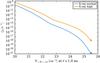 |
Fig. A.1 X-ray ionization rate ζX as a function of vertical hydrogen column density of the disk at a distance of 1 au from the star. Shown are the resulting ionization rates for the two different X-ray spectra (see Sect. 2.3.1). The dots mark the same location (r = 1 au, z = 0 au) in the disk as the dots in Fig. A.2. |
Here we have used the newly developed X-ray radiative transfer module of PRODIMO. The details of this module will be presented in a forthcoming paper Rab et al. (in prep.). Here we only briefly describe the implementation and present results concerning the X-ray ionization rate for comparison with other models.
The main difference between the new model and the existing implementation of Aresu et al. (2011), Meijerink et al. (2012) is the treatment of X-ray scattering. We used the absorption and scattering cross-section from the publicly available xraylib library1 (Schoonjans et al. 2011). For the X-ray radiative transfer we use the same numerical approach (e.g. use of wavelength bands) as is used for the dust radiative transfer in PRODIMO (Woitke et al. 2009). We assumed isotropic scattering but applied a correction factor (anisotropic factor g) to account for anisotropic Compton scattering. According to Cleeves et al. (2016), neglecting anisotropic scattering has only a limited impact on the X-ray ionization rate of about a factor of two. We consider this possible deviation as not significant for the results presented here. We further disregarded the dust in the X-ray radiative transfer, since with the assumed gas to dust ratio of 100 and dust settling X-ray photons mainly interact with the gas (Bethell & Bergin 2011; Glassgold et al. 2012).
The X-ray chemistry in PRODIMO is presented in detail in Meijerink et al. (2012). The interaction of X-rays with the gas changes the species abundances and consequently also the X-ray opacities. We therefore iterated between the X-ray radiative transfer and the chemistry until convergence is reached.
In Figs. A.1 and A.2 we show the X-ray ionization rate ζX for our disk model (Sect. 2.4) and for both X-ray spectra (Sect. 2.3.1). Figure A.1 shows ζX as a function of vertical column density at 1 au whereas Fig. A.2 shows ζX in the midplane of the disk as a function of radius. These results are in good quantitative agreement with Ercolano & Glassgold (2013) and Cleeves et al. (2015) considering that different disk models and different implementations of X-ray radiative transfer (e.g. cross-sections) are applied.
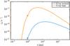 |
Fig. A.2 X-ray ionization rate ζX as a function of radius in the midplane of the disk (z = 0). Shown are the resulting ionization rates for the two different X-ray spectra (see Sect. 2.3.1). The dots mark the same location (r = 1 au, z = 0 au) in the disk as the dots in Fig. A.1. |
Appendix B: Chemistry
Rate coefficients for the main formation and destruction pathways of HCO+ and N2H+.
For the chemical reaction network we use the UMIST 2012 database for gas phase chemistry (McElroy et al. 2013) for a selection of 235 species. Additionally the network includes X-ray chemistry (Aresu et al. 2011; Meijerink et al. 2012), PAH (polycyclic aromatic hydrocarbons) chemistry (Thi et al. 2014), adsorption and desorption (thermal, CR and photo desorption) for ice species and H2 formation on grains (Woitke et al. 2009). In total the network includes 3143 chemical reactions. For the ice species we use the binding energies from the UMIST 2012 release but updated a couple of values for oxygen bearing species (see Sect. B.2). Further details on the network can be found in Kamp et al. (2017). The most relevant gas phase reactions for HCO+ and N2H+ with their rate coefficients are listed in Table B.1.
To test the robustness of our chemical model with respect to HCO+ and N2H+ we performed chemical tests with time-dependent chemistry, varying binding energies and the KIDA chemical network (Kinetic Database for Astrochemistry, Wakelam et al. 2012, 2015). The different test models are described in Table B.2 and discussed in the following sections. The results for the HCO+ and N2H+ column densities are shown in Figs. B.1 and B.2.
Appendix B.1: N2 shielding
Dust shielding of N2 photodissociation is strongly reduced in protoplanetary disks due to dust evolution (e.g. dust growth) and shielding by H2 becomes important (Li et al. 2013). To account for this we implemented the H, H2 shielding and self-shielding functions for N2 of Li et al. (2013) in our chemistry model. The data are taken from the Leiden photodissociation database2 .
We find that N2 shielding is very important for the abundance structure of N2H+. In models without N2 shielding the vertical column density of N2H+ is reduced by one order of magnitude throughout the disk. Further the warm N2H+ layer above the vertical CO ice-line vanishes.
Chemical test models.
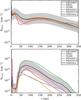 |
Fig. B.1 Comparison of column densities for HCO+ and N2H+ for models with different chemical networks or binding energies (see Table B.2). The grey shaded area marks a difference of a factor 3 in the column densities relative to the reference model (black line). |
Appendix B.2: Binding energies
Appendix B.2.1: Oxygen binding energy
Several laboratory experiments (e.g. Ward et al. 2012; He et al. 2014; Minissale et al. 2016a,b) reported binding energies for oxygen in the range of EB(O) = 1500 − 1800 K. This is significantly higher than the value of EB(O) = 800 K listed in the UMIST 2012 database. We therefore updated the binding energies for oxygen and several other oxygen bearing species with the values listed in Minissale et al. (2016b). The new values with their references are given in Table B.3.
The higher binding energy for oxygen has a significant impact on N2H+. Using the UMIST 2012 binding energy reduces the N2H+ column density by about a factor of three for r ≳ 50 au (see model EBUMIST in Fig. B.1). Similar to CO, oxygen also destroys N2H+ via the reaction O + N2H+ → N2 + OH+. Due to this reaction the N2H+ abundance is strongly reduced in a thin layer below the vertical CO ice line and above the vertical oxygen ice line. With the higher binding energy for oxygen this thin layer vanishes as oxygen freezes-out at higher temperatures than CO.
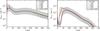 |
Fig. B.2 Comparison of time-dependent and steady-state chemistry models. Shown are the vertical column densities for HCO+ and N2H+ at different chemical ages of the disk (colored lines) and the steady-state results (black line). The grey shaded area marks a difference of a factor 3 in the column densities relative to the steady-state model. |
Important binding energies.
For HCO+ the dip in the column density profile at r ≈ 50 au alone is significantly affected. In this region HCO+ is efficiently destroyed by water. Removing oxygen and OH from the gas phase reduces also the water abundance near the vertical CO ice line, consequently the HCO+ abundance increases.
Appendix B.2.2: N2 binding energy
In the UMIST 2012 database EB(N2) = 0.67 × EB(CO) (see Table B.3). This ratio is close to the value of 0.65 used to explain observations of prestellar cores showing that N2 freezes out at lower temperatures than CO (e.g. Bergin & Langer 1997; Bergin et al. 2001; Ceccarelli & Dominik 2005). Also disk observations of N2H+ indicate that EB(N2) <EB(CO) (Qi et al. 2003, 2013b). However, the ratio of 0.65 is in contradiction with laboratory experiments which show EB(N2) ≈ 0.9 × EB(CO) (Öberg et al. 2005; Bisschop et al. 2006; Fayolle et al. 2016). One explanation for this discrepancy might be differential freeze-out but it is unclear if this is sufficient (Bisschop et al. 2006; Fayolle et al. 2016).
In our models the N2H+ column density drops by about one order of magnitude if we set EB(N2) = 0.9 × EB(CO) (model EBN2 in Fig. B.1). Contrary to our model Aikawa et al. (2015) find that in their disk model the N2H+ abundance structure is not strongly affected by setting EB(N2) = EB(CO). They argue that due to the sink effect, CO is depleted anyway and therefore the N2H+ abundance is not strongly affected by setting EB(N2) = EB(CO). We have not included dust surface chemistry in our model therefore the CO sink effect is less efficient. Aikawa et al. (2015) argue that the sink effect depends on various parameters (turbulence in the disk, efficiency of the conversion of CO to less volatile species) therefore they also studied a no-sink model. In this no-sink model the N2H+ abundance is sensitive to the binding energy of N2, very similar to our models.
The main difference between the sink and no-sink model is the location of the CO ice line and the N2H+ layer. In the sink model CO is also depleted at temperatures higher than its sublimation temperature, consequently the CO ice line moves to higher and warmer layers of the disk. In the no-sink model the CO ice line is given by the adsorption/desorption equilibrium for CO which depends on the chosen CO binding energy. However, with the exception of the exact location of the CO ice line and the N2H+ layer our models with EB(N2) = 0.67 × EB(CO) are in good agreement with the full chemical network/sink model of Aikawa et al. (2015). We discuss the impact of the CO ice line location on our results in Sect. 4.2.1.
Appendix B.3: Comparison to the KIDA chemical network
The reaction rates for nitrogen chemistry are not as well known as for carbon/oxygen chemistry (e.g. Hily-Blant et al. 2010; Le Gal et al. 2014). Wakelam et al. (2013) reviewed a large number of important reactions for nitrogen chemistry. The new derived reactions rates are in included in the latest KIDA gas phase chemistry database release (Wakelam et al. 2015).
We ran models using the KIDA gas phase chemistry database instead of the UMIST 2012 database (see Table B.2). We used the KIDA 2011 (Wakelam et al. 2012) and the KIDA 2014 (Wakelam et al. 2015) releases. The additional chemistry included in PRODIMO (e.g. X-ray chemistry) remains the same.
Figure B.1 shows the resulting HCO+ and N2H+column densities for the KIDA2011 and KIDA2014 model in comparison to the reference model (UMIST 2012). In the KIDA2011 model the N2H+ column density is about a factor of three higher compared to the reference and KIDA2014 models. The reason are updated rate coefficients for the dissociative recombination reactions of N2H+ with electrons. The reaction rates at 20 K for N2H+ + e− → N2 + H (N2H+ + e− → NH + N) are a about a factor of five (three) higher in the KIDA 2014/UMIST 2012 releases than in the KIDA 2011 release. This explains the higher N2H+ abundance in the KIDA 2011 model. However, we find a good agreement for the KIDA 2014 and the UMIST 2012 release for both molecules HCO+ and N2H+.
Appendix C: Steady-state versus time-dependent chemistry
For our models we have assumed that the chemistry reaches a steady-state within typical lifetimes of disks (couple of million years). To verify this assumption we run time-dependent chemistry models for the reference models CI_XN and CL_XN. We find that for the species considered in this work HCO+ and N2H+ the chemistry reaches steady-state within ≈1 Myr in a large fraction of the disk. This is in agreement with the models of Aikawa et al. (2015) although they use a different, in particular larger chemical network.
In Fig. B.2 we compare the vertical column densities NHCO+ and NN2H+ of the steady-state model to the results of the time-dependent models at different times. For r ≳ 30 au and t ≳ 1 Myr to column densities of the steady-state and the time-dependent model are nearly identical. However, the steady-state model underestimates NHCO+ and NN2H+ for r ≲ 30 au. The differences are caused by the “sink effect” for CO and N2 (see Sect. 3.3 and Aikawa et al. 2015). This erosion of CO and N2 and other neutral molecules in the disk midplane by the reaction with He+ is a slow chemical process (e.g. Furuya & Aikawa 2014; Bergin et al. 2014; Helling et al. 2014) and is therefore over-estimated in the steady-state models.
As N2H+ resides in deeper layers than HCO+ the deviations in the column densities are more pronounced. As a consequence the N2H+ column density does not exactly trace the CO ice line in the midplane of the disk. The midplane CO ice line is located at r ≈ 12 au in the time-dependent model, whereas in the steady-state model NN2H+ indicates a CO ice line at r ≈ 30 au. We note that in the low CR model CL_XN the sink effect is less efficient due to the lower midplane ionization rate, therefore the deviations in the steady-state models for NHCO+ and NN2H+ are smaller (NN2H+ indicates a CO ice line at r ≈ 20 au).
Our comparison shows that for the bulk of NHCO+ and NN2H+ the assumption of steady-state chemistry is well justified. In particular our conclusions concerning the impact of SP ionization are not affected by the artifacts in the steady-state models. A steady-state model requires about a factor of ten less computational time than the time-dependent models. The use of the steady-state models allows us to study other important aspects like the impact of CO depletion (Sect. 4.2.2) or the comparison of different chemical networks.
Appendix D: The Turner model
In Turner & Drake (2009) the SP ionization rate is calculated for a mean solar mass nebulae disk model. To calculate the SP ionization rate at the surface of the disk they scaled their CR ionization rate of ζCR = 5 × 10-18 s-1 by a factor of 104(r/ au)-2. To account for the attenuation of SPs as a function of hydrogen column density they applied the same equation as they use for Galactic cosmic rays (their Eq. (2)).
To compare our results with the approach of Turner & Drake (2009) we implemented their method in our model. We also used their X-ray input spectrum and applied our X-ray radiative transfer to calculate the X-ray ionization rate. In Fig. D.1 we show the resulting X-ray, SP and CR ionization rates as a function of radius at a vertical column density of ≈8 g cm-2 (≈3 × 1024 cm-2) for the Turner model (CI_T) and for our CI_XN_SP model. A comparison of Fig. D.1 with Fig. 1 of Turner & Drake (2009) shows that the CI_T model reproduces their SP ionization rates. We note that in our disk model (i.e lower disk mass) only for r< 10 au a vertical column density of >3 × 1024 cm-2 is reached; therefore only the inner 10 au are shown.
Figure D.1 clearly shows the differences of the two approaches. In our models SPs can only penetrate the disk radially and therefore cannot reach the disk midplane (see Sect. 3.2). In the Turner model the particles can also penetrate the disk vertically down to the midplane as they use the same equation for SP attenuation as is used for Galactic CRs. We cannot reproduce their results if we allow only for radial transport of particles. The differences in the X-ray ionization rate are due to the different X-ray spectrum (LX = 2 × 1030 erg s-1,TX = 5.8 × 10⁷ K, see Table 2) used by Turner & Drake (2009).
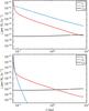 |
Fig. D.1 Ionization rates at a vertical column density of N⟨ H ⟩ ,ver = 3.4 × 1024 cm-2 (≈8 g cm-2) as a function of distance to the star. The top panel shows the Turner model (CI_T), the bottom panel the CI_XN_SP model (see Table 5). |
Appendix E: Comparison to observations
We compared the HCO+J = 3 − 2 and N2H+J = 3 − 2 line fluxes from our reference model to the observations of Öberg et al. (2010, 2011a). From their sample we choose the targets where both lines were detected (the six targets shown in Fig. 6 of Öberg et al. 2011a). The observed integrated line fluxes are in the range of 3.1 − 17.8 Jy km s-1 for HCO+J = 3 − 2 and in the range of 0.4 − 2.9 Jy km s-1 for N2H+J = 3 − 2 (all line fluxes are scaled to a distance of 140 pc). Excluding IM Lup, an extremely large and massive disk, from the sample gives a much narrower range of 3.1 − 5.4 Jy km s-1 and 0.4 − 1.4 Jy km s-1 for HCO+J = 3 − 2 and N2H+J = 3 − 2, respectively.
To calculate the line fluxes for our model we use the line transfer module of PRODIMO (Woitke et al. 2011) and the molecular data from the Leiden Atomic and Molecular Database (Schöier et al. 2005; Botschwina et al. 1993; Flower 1999). For our reference model CI_XN we find fluxes of 2.4 Jy km s-1 and 0.78 Jy km s-1 for HCO+J = 3 − 2 and N2H+J = 3 − 2, respectively. As the sample of Öberg et al. (2011a) is probably biased towards large and massive disks we also calculated the fluxes for a disk four times more massive. We find fluxes of 4.3 Jy km s-1 and 1.18 Jy km s-1 for HCO+J = 3 − 2 and N2H+J = 3 − 2, respectively. These results are well within the range of the observations.
All Tables
Fitting parameters for the stellar particle ionization rate for the two different input spectra.
Rate coefficients for the main formation and destruction pathways of HCO+ and N2H+.
All Figures
|
Fig. 1 Stellar particle (proton) spectra for five different solar particle events. Shown are fits to the measurements presented in Mewaldt et al. (2005). |
| In the text | |
|
Fig. 2 Stellar energetic proton (SP) and cosmic-ray (CR) input spectra. The blue solid and dashed lines show the active Sun and active T Tauri SP spectrum, respectively. The black solid line shows the “LIS W98” CR spectrum from Webber (1998) and the dashed black line the attenuated “Solar Max” CR spectrum from Cleeves et al. (2013). |
| In the text | |
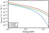 |
Fig. 3 Stellar X-ray input spectra (see Table 2). |
| In the text | |
|
Fig. 4 Two dimensional structure of the reference disk model CI_XN. The height of the disk z is scaled by the radius (z/r). From top left to the bottom right: a) gas number density n⟨ H ⟩; b) dust density ρdust (note the dust settling); c) FUV radiation field χ in units of the ISM Draine field; d) gas temperature Tgas; e) dust temperature Tdust and f) the vertical hydrogen column density N⟨ H ⟩ ,ver versus radius. The white dashed contour lines in each contour plot correspond to the levels shown in the respective colorbar. The black (red) solid contour in panel c) indicate a vertical (radial) visual extinction equal to unity. |
| In the text | |
|
Fig. 5 SP, CR and X-ray ionization rates ζ as a function of hydrogen column density N⟨ H ⟩. |
| In the text | |
|
Fig. 6 Ionization rates ζ as a function of vertical column density N⟨ H ⟩ ,ver at radii of 1 and 100 au (solid and dashed lines respectively). The maximum values for N⟨ H ⟩ ,ver at the midplane of the disk, are N⟨ H ⟩ ,ver ≈ 4 × 1025 cm-2 and N⟨ H ⟩ ,ver ≈ 2 × 1023 cm-2 at 1 au and 100 au, respectively. Red lines are for X-rays, blue lines are for SPs and the black lines are for CRs. Left panel: model CI_XN_SP with ISM CRs and normal X-rays; right panel: model CL_XH_SP with low CRs and high X-rays. |
| In the text | |
|
Fig. 7 Dominant disk ionization source throughout the disk. A light grey area indicates a region without a dominant ionization source. The different possible ionization sources, X-rays, SPs and CRs are identified by the different colors (color bar). The white solid contour line shows N⟨ H ⟩ ,rad = 1025 cm-2 the white dashed line shows the CO ice line. The model names are given in the top left of each panel. Top row: models with ISM CR ionization rate (CI); bottom row: models with low CR ionization rate (CL). First column: normal X-ray models (XN); second column: high X-ray models (XH); third column: turner models (T). |
| In the text | |
|
Fig. 8 Abundances ϵ(X) relative to hydrogen for CO, HCO+ and N2H+ for the reference model CI_XN. The white solid contour line shows N⟨ H ⟩ ,rad = 1025 cm-2, the white dashed line shows the CO ice line. We call the regions above and below the CO ice line the warm and cold molecular layer, respectively. The dotted iso-contours show where the X-ray ionization rate is equal to the ISM CR (ζCR = 2 × 10-17 s-1) and equal to the low CR (ζCR = 2 × 10-19 s-1) ionization rate, respectively. |
| In the text | |
|
Fig. 9 Vertical column density profiles for HCO+ and N2H+ for our model series (Table 5). The left column shows the models with the ISM like CRs (ζCR ≈ 2 × 10-17 s-1), the right column with low CRs (ζCR ≈ 2 × 10-19 s-1). The top row shows HCO+, the bottom row N2H+. The blue lines are for models with, the red lines are for models without SPs. Dashed (solid) lines are for models with high (normal) X-rays. The orange solid line shows the Turner model. The grey shaded area marks a difference of a factor 3 in the column densities relative to the CI_XN (ISM CR, normal X-rays) and CL_XN model (low CR, normal X-rays), respectively. |
| In the text | |
|
Fig. 10 Ionization rate weighted column densities Nζ (Eq. (5)) as a function of radius for HCO+ (left column) and N2H+ (right column). Nζ is normalized to the total column density of the respective molecule. The individual colored solid lines show the fraction of the total column density dominated by a certain ionization source. Red is for X-rays (NζX), blue for SPs (NζSP) and black for CRs (NζCR). Each row corresponds to one model. On the right hand side the model descriptions are provided (see Table 5). The grey shaded area marks the region where more than 50% of the column density arise from regions above the CO ice line (i.e. the warm molecular layer). |
| In the text | |
|
Fig. 11 Comparison of column densities for HCO+ (top) and N2H+ (bottom) for models with varying SP flux and very strong X-ray emission. For all models the low CR ionization rates are used. Shown are the reference model with normal X-rays (black, CL_XN), the model with the typical SP flux (blue, CL_XN_SP) and models with a factor of ten higher (purple, CL_XN_SPH) and factor of ten lower (red, CL_XN_SPL) SP flux. The dashed black line shows the model with LX = 3 × 1031 erg s-1 and no SPs. The grey shaded area marks a difference of a factor of three in the column densities relative to the reference model CL_XN. |
| In the text | |
|
Fig. A.1 X-ray ionization rate ζX as a function of vertical hydrogen column density of the disk at a distance of 1 au from the star. Shown are the resulting ionization rates for the two different X-ray spectra (see Sect. 2.3.1). The dots mark the same location (r = 1 au, z = 0 au) in the disk as the dots in Fig. A.2. |
| In the text | |
|
Fig. A.2 X-ray ionization rate ζX as a function of radius in the midplane of the disk (z = 0). Shown are the resulting ionization rates for the two different X-ray spectra (see Sect. 2.3.1). The dots mark the same location (r = 1 au, z = 0 au) in the disk as the dots in Fig. A.1. |
| In the text | |
|
Fig. B.1 Comparison of column densities for HCO+ and N2H+ for models with different chemical networks or binding energies (see Table B.2). The grey shaded area marks a difference of a factor 3 in the column densities relative to the reference model (black line). |
| In the text | |
|
Fig. B.2 Comparison of time-dependent and steady-state chemistry models. Shown are the vertical column densities for HCO+ and N2H+ at different chemical ages of the disk (colored lines) and the steady-state results (black line). The grey shaded area marks a difference of a factor 3 in the column densities relative to the steady-state model. |
| In the text | |
|
Fig. D.1 Ionization rates at a vertical column density of N⟨ H ⟩ ,ver = 3.4 × 1024 cm-2 (≈8 g cm-2) as a function of distance to the star. The top panel shows the Turner model (CI_T), the bottom panel the CI_XN_SP model (see Table 5). |
| In the text | |
Current usage metrics show cumulative count of Article Views (full-text article views including HTML views, PDF and ePub downloads, according to the available data) and Abstracts Views on Vision4Press platform.
Data correspond to usage on the plateform after 2015. The current usage metrics is available 48-96 hours after online publication and is updated daily on week days.
Initial download of the metrics may take a while.