| Issue |
A&A
Volume 602, June 2017
|
|
|---|---|---|
| Article Number | A32 | |
| Number of page(s) | 14 | |
| Section | Stellar structure and evolution | |
| DOI | https://doi.org/10.1051/0004-6361/201730571 | |
| Published online | 31 May 2017 | |
Kepler sheds new and unprecedented light on the variability of a blue supergiant: Gravity waves in the O9.5Iab star HD 188209⋆
1 Instituut voor Sterrenkunde, KU Leuven, Celestijnenlaan 200D, 3001 Leuven, Belgium
e-mail: This email address is being protected from spambots. You need JavaScript enabled to view it.
2 Department of Astrophysics/IMAPP, Radboud University Nijmegen, 6500 GL Nijmegen, The Netherlands
3 Instituto de Astrofísica de Canarias, 38200 La Laguna, Tenerife, Spain
4 Departamento de Astrofísica, Universidad de La Laguna, 38205 La Laguna, Tenerife, Spain
5 NASA Ames Research Center, Moffett Field, CA 94095, USA
6 Bay Area Environmental Research Institute, 560 Third Street W., Sonoma, CA 95476, USA
7 Center of Excellence in Information Systems, Tennessee State University, 3500 John A. Merritt Blvd., Box 9501, Nashville, TN 37209, USA
8 Stellar Astrophysics Centre, Department of Physics and Astronomy, Aarhus University, 8000 Aarhus C, Denmark
9 Department of Mathematics and Statistics, Newcastle University, Newcastle upon Tyne NE1 7RU, UK
10 Planetary Science Institute, Tucson, AZ 85721, USA
Received: 6 February 2017
Accepted: 3 March 2017
Abstract
Stellar evolution models are most uncertain for evolved massive stars. Asteroseismology based on high-precision uninterrupted space photometry has become a new way to test the outcome of stellar evolution theory and was recently applied to a multitude of stars, but not yet to massive evolved supergiants.Our aim is to detect, analyse and interpret the photospheric and wind variability of the O9.5 Iab star HD 188209 from Kepler space photometry and long-term high-resolution spectroscopy. We used Kepler scattered-light photometry obtained by the nominal mission during 1460 d to deduce the photometric variability of this O-type supergiant. In addition, we assembled and analysed high-resolution high signal-to-noise spectroscopy taken with four spectrographs during some 1800 d to interpret the temporal spectroscopic variability of the star. The variability of this blue supergiant derived from the scattered-light space photometry is in full in agreement with the one found in the ground-based spectroscopy. We find significant low-frequency variability that is consistently detected in all spectral lines of HD 188209. The photospheric variability propagates into the wind, where it has similar frequencies but slightly higher amplitudes. The morphology of the frequency spectra derived from the long-term photometry and spectroscopy points towards a spectrum of travelling waves with frequency values in the range expected for an evolved O-type star. Convectively-driven internal gravity waves excited in the stellar interior offer the most plausible explanation of the detected variability.
Key words: techniques: photometric / techniques: spectroscopic / stars: massive / waves / stars: oscillations / stars: individual: HD 188209
Based on photometric observations made with the NASA Kepler satellite and on spectroscopic observations made with four telescopes: the Nordic Optical Telescope operated by NOTSA and the Mercator Telescope operated by the Flemish Community, both at the Observatorio del Roque de los Muchachos (La Palma, Spain) of the Instituto de Astrofísica de Canarias, the T13 2.0 m Automatic Spectroscopic Telescope (AST) operated by Tennessee State University at the Fairborn Observatory, and the Hertzsprung SONG telescope operated on the Spanish Observatorio del Teide on the island of Tenerife by the Aarhus and Copenhagen Universities and by the Instituto de Astrofísica de Canarias, Spain.
© ESO, 2017
1. Introduction
Stars born with sufficiently high mass to explode as supernova at the end of their life have major impact on the dynamical and chemical evolution of galaxies. Appropriate models of such pre-supernovae are thus highly relevant for astrophysics. Unfortunately, the theory of their evolution is a lot less well established than that of low-mass stars that die as white dwarfs. Differences in the predictions of massive star evolution from various modern stellar evolution codes even occur already well before the end of the main-sequence (MS) phase (e.g. Martins & Palacios 2013).
Despite the immense progress in the asteroseismic tuning of stellar models of various types of stars from high-precision uninterrupted space photometry in the past decade (e.g. Chaplin & Miglio 2013; Charpinet et al. 2014; Aerts 2015; Hekker & Christensen-Dalsgaard 2016, for reviews), we still lack suitable data to achieve this stage for massive O-type stars and their evolved descendants, the B supergiants. Indeed, while the MOST and CoRoT missions observed a few B supergiants for weeks to months (e.g. Saio et al. 2006; Aerts et al. 2010, 2013; Moravveji et al. 2012), their pulsational frequencies were not measured with sufficient precision and/or the angular wavenumbers (ℓ,m) of their oscillation modes could not be identified (e.g. Aerts et al. 2010, for a detailed description of mode identification in asteroseismology). Despite appreciable efforts, a similar situation occurred for the earlier phases, given the absence of suitable highly sampled space photometric data with sufficiently long time bases for O stars (see e.g. Buysschaert et al. 2015, for an updated summary). Hence, improvement of the input physics adopted in stellar models representing various evolutionary phases of massive stars is still beyond reach, in contrast to such achievements for low-mass stars (e.g. Bedding et al. 2011; Bischoff-Kim & Østensen 2011; Foster et al. 2015; Deheuvels et al. 2015, to mention just a few studies).
There are several reasons why asteroseismology of evolved stars in the mass range of supernova-progenitors, i.e. with birth masses above some 8 M⊙, is so difficult to achieve. First and foremost, such stars have large radii and connected with this, their oscillation periods are several to tens of days. Any multiperiodic non-radial mode beating pattern therefore reaches periods of years and such a time base is beyond the capacity of the MOST, CoRoT, and K2 space missions. This is also the reason why gravity-mode pulsators in the core-hydrogen burning phase, which have periods of the order of half to a few days, could only be fully exploited seismically thanks to the nominal Kepler mission. Indeed, although their period-spacing pattern was first discovered from 150 d of uninterrupted CoRoT data (Degroote et al. 2010), seismic modelling of MS gravity-mode pulsators required at least a year of uninterrupted space photometry. Four years of Kepler data of B and F stars led to interior structure properties that cannot be explained with standard models, in terms of interior rotation and mixing (e.g. Kurtz et al. 2014; Saio et al. 2015; Moravveji et al. 2015, 2016; Triana et al. 2015; Murphy et al. 2016; Van Reeth et al. 2016; Schmid & Aerts 2016). It is thus to be expected that models of their evolved counterparts deviate even more from reality.
A second reason that hampers asteroseismology of O stars and B supergiants is the fact that their variability is not only caused by heat-driven coherent stellar oscillations, but also by a time-variable radiation-driven stellar wind, rotational effects, macroturbulence, and for very few of the youngest O stars magnetic activity as well (Fossati et al. 2016). All these physical phenomena interact, often non-linearly and in a non-adiabatic regime. This leads to complex overall variability with even longer time bases than a classical multiperiodic oscillation.
Here, we present a study of HD 188209 (O9 Iab), the only massive supergiant that was monitored with the nominal Kepler mission during a total time base of four years and about equally long in ground-based spectroscopy. We first introduce the known properties of our target star and then discuss long-term monitoring in space photometry and ground-based spectroscopy. We provide, in independent data sets, evidence for variability with an entire spectrum of periods of the order of half to a few days.
Spectroscopically derived properties of HD 188209 reported in the recent literature based on a non-LTE analysis.
2. The O9 Iab supergiant HD 188209
Given its visual magnitude of 5.63, HD 188209 was the subject of various observational variability studies so far. These mainly focused on spectroscopy and were limited to only few spectra gathered with low sampling rates. Early spectroscopic time series assembled by Fullerton et al. (1996) and Israelian et al. (2000) revealed line-profile variability in the UV and optical parts of its spectrum, with various timescales of the order of days. Additional studies by Markova et al. (2005), Fullerton et al. (2006), and Martins et al. (2015a) revealed variability in both the photosphere and stellar wind, with seemingly uncorrelated quasi-periodicities occurring in those two regimes.
The spectral type assigned to HD 188209 is O9.5Iab (Walborn 1972; Sota et al. 2011). It is included in the list of standard stars for spectral classification (e.g. Walborn & Fitzpatrick 1990; Maíz Apellániz et al. 2015. The fundamental parameters, mass-loss rate, and level of macroturbulence from recent analyses based on the non-LTE codes CMFGEN (Martins et al. 2015a,b) and FASTWIND (Markova et al. 2005; Holgado et al., in prep.), both including the effects of line blanketing and the stellar wind, are listed in Table 1. While binarity dominates the evolution of massive stars (Sana et al. 2012), HD 188209 was found to be a single star (Martins et al. 2015b). In line with the low incidence of surface magnetic fields in OB stars, HD 188209 led to a non-detection of such a field (Grunhut et al. 2017).
Given its presence in the nominal field of view (FoV) of the Kepler satellite, we have embarked on a unique long-term monitoring study of HD 188209, based on space photometry and ground-based high-resolution spectroscopy.
3. Scattered-light Kepler photometry
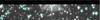 |
Fig. 1 Position of the two apertures (45: left), 32 (right) in the Kepler FoV capturing the scattered light of HD 188209 (situated in the black band above the red cross in between active silicon). |
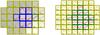 |
Fig. 2 Example of pixel masks used to create three versions of the light curves for star 45 (left) and 32 (right). The detected light curve is plotted within each pixel and represents an addition of 270 individual exposures of 6.54 s, added on board of the satellite. In long-cadence mode, such pixel data are downloaded from the spacecraft in time stamps of 29.42 min. The values listed in every pixel indicate the S/N level of the flux in the pixel. The red dots in the pixels with green and blue borders were used to extract the standard Kepler light curves. We also computed light curves based on the data in the yellow pixels alone and from adding the green, blue, and yellow pixels. |
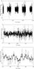 |
Fig. 3 Light curves in masks 32 (grey circles) and 45 (black circles) covering the full length (upper), quarters 4 and 5 (middle) and a zoom of 20 d. |
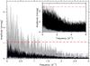 |
Fig. 4 Amplitude spectrum for the Kepler light curves of masks 32 (grey) and 45 (black). The inset compares the spectrum of the Kepler light curve from mask 32 (grey) with the Hipparcos light curve (black) over twice the frequency range. The red dashed and blue dot-dot-dot-dashed lines indicate four times the average noise level computed over the frequency range [0,6] d-1, while the red dot-dashed line in the inset represents four times the average noise level computed over the same range [0,6] d-1 of the Hipparcos data. |
The Kepler CCDs saturate for Kp ~ 11.5, the precise value depending on the CCD and target location on that CCD (Koch et al. 2010). However, it turned out that the saturated flux is conserved to a very high degree as long as sufficiently large masks are placed around the star under study. This led to several variability studies of bright stars with unprecedented photometric precision and duration of light curves by means of customised masks (e.g. Kolenberg et al. 2011; Metcalfe et al. 2012; Tkachenko et al. 2014; Guzik et al. 2016). Meanwhile, numerous bright stars have also been studied with the refurbished Kepler mission K2 by co-adding carefully masked smear flux in the CCD rows of data taken with ultra-short exposure times (White et al. 2017); this technique was verified successfully on nominal Kepler data (e.g. Pope et al. 2016).
Here, we present a different use of the original Kepler satellite, following our idea to perform scattered-light aperture photometry of HD 188209, even though the star is not on active silicon. With Kp~5.5, HD 188209 was indeed a nuisance for exoplanet hunting with the nominal Kepler mission and it was therefore placed carefully in between the active CCDs pointing to the nominal FoV. Nevertheless, it is so bright that its scattered light does “pollute” the CCDs (cf. Fig. 1). As only targets on active silicon are eligible for the Kepler and K2 Guest Observer programmes, we had to proceed in a different way and informally requested the Kepler GO office to place masks in the vicinity of HD 188209 with the reasoning that its variability behaviour would be present and detectable in the scattered-light photometry.
For the current analysis, we used two apertures placed in the scattered light of the star. The two masks placed on active silicon correspond to the targets labelled KIC 10092932 (to the right) and KIC 10092945 (to the left) of HD 188209 in Fig. 1, hereafter called mask 32 and mask 45, respectively. Mask 45 contains a faint star of Kp~13.35, which is 7.85 mag fainter than HD 188209 itself; mask 32 does not contain any known source and is therefore a pure probe of the scattered light of the supergiant. Mask 32 has Kp = 11.2 as brightness for the scattered light. Both these masks were observed in long-cadence (LC) mode with a total integration time of 29.42 min per data point. Each downloaded LC flux value is an on-board addition of 270 individual exposures of 6.54 s, with 0.52 s readout time.
Masks of a selected Kepler quarter showing the light curves in the individual pixels as downloaded from the spacecraft for each of the two apertures are shown in Fig. 2. These show the typical time series traces with pixel-to-pixel variations as for normal targeted stars (e.g. Pápics et al. 2014), except that the flux levels are lower here. This is particularly the case for mask 32 given that it concerns scattered light rather than an actual target. The signal-to-noise ratio (S/N) of the detected flux in every pixel is indicated in each of the boxes. We used the pixels with dark green or blue borders with red dots shown as flux values (stored in e− s-1) to extract the standard Kepler light curves of targets as provided in MAST1. We not only used these light curves but also constructed two new ones that are based on the yellow pixels in which significant signal coming from the supergiant is present as well; S/N values above 100 typically correspond to useful signal to be added for stellar variability studies. Adding the flux in those yellow pixels in addition to the standard MAST pixels leads to cleaner detrending and less contamination by instrumental effects at low frequencies (Tkachenko et al. 2013; Pápics et al. 2014). For each of the two custom masks, we extracted two light curves in addition to the standard MAST curves: one based on the yellow flux alone and another one based on the green, blue, and yellow flux. For each of the two masks, the variability behaviour of these three light curves is the same in terms of periodic behaviour, which is evidence that this variability is dominated by the scattered light of the supergiant and not by other sources in the pixel masks.
In the rest of the paper, we proceed with the light curves containing maximal S/N. These light curves are deduced from adding all the flux in the red, blue, and yellow pixels of masks 32 and 45 as shown in Fig. 2. Figure 3 compares these two light curves, in which mask 45 was observed during 1460 d from 13/5/2009 until 9/4/2013 (quarters 1, 4, 5, 8, 9, 12, 13, 16, 17; in total 31 034 measurements) and mask 32 during 1147 d from 20/3/2010 until 9/4/2013 (quarters 5, 13, 17; in total 10 080 measurements). Even though it is scattered light, this is by far the best light curve ever obtained for a blue supergiant. The lower panel of Fig. 3 shows that the two curves are very similar in terms of temporal variability, but that the amplitude of the variability is different. This is as expected given the difference in flux level within the masks and the fact that mask 45 contains a faint star while mask 32 does not.
We computed the Fourier transform of the two light curves shown in Fig. 3 to obtain the amplitude spectra up to the Nyquist frequency. This resulted in a flat distribution of noise beyond 6 d-1 and a clear amplitude excess above the noise level at low frequency for both light curves. A part of the spectrum is shown in Fig. 4, where the horizontal lines are situated at four times the average noise level computed over the range [0,6] d-1. Given that mask 32 is the “purer” one in terms of only scattered light of HD 188209, its amplitude is dominant over the one obtained from mask 45. However, both light curves are fully consistent with each other in the sense that significant variability is detected over the whole frequency range [0,2] d-1 in the form of an excess of amplitude for numerous close frequencies. This is a frequency regime typical for gravity waves in massive stars.
The amplitude spectrum in Fig. 4 is entirely different in nature from that of the rotationally variable B5 supergiant HD 46769 observed with CoRoT during 23 d, revealing only one frequency and its harmonics corresponding to a rotation period of 4.8 ±0.2 d (Aerts et al. 2013). It also bears no resemblance to the frequency spectrum of the B6 supergiant HD 50064 whose 137-d CoRoT light curve revealed one dominant radial pulsation mode with a period of 37 d, identified as the fundamental radial mode of the star (Aerts et al. 2010). The morphology of the spectrum is also different from those found for Kepler data of B dwarfs pulsating in coherent heat-driven gravity modes (e.g., Pápics et al. 2015, 2017) and from those of O dwarfs with variability assigned to rotational modulation or heat-driven coherent non-radial pulsations (see Table 3 in Buysschaert et al. 2015, for an overview).
Since we are dealing with a photometric curve deduced from scattered light, a comparison with other photometric data of the actual star is meaningful. The only publicly available light curve of HD 188209 to make such a comparison is the light curve assembled by the Hipparcos satellite, which is of similar total length but has only 113 data points spread over 1156 d with far less precision than the Kepler scattered light data. This data set was already analysed by Israelian et al. (2000, see their Fig. 3) and revealed variability but did not lead to clear periodicity. We recomputed the amplitude spectrum of the Hipparcos light curve and compared it with the Kepler light curve of mask 32, which is similar in length, in the inset of Fig. 4. Although the significance of the amplitude excess in the Hipparcos data is only marginal at best, low-frequency excess in [0,2] d-1 is also hinted at in this independent photometric data set at a level of some 14 mmag, while we found 3.6 mmag from the scattered light in mask 32.
The photometric amplitude spectrum of the scattered light of HD 188209 is remarkably similar to that obtained from the Kepler data of the bright primary B0 III star (Lesh 1968) of the eclipsing binary V380 Cyg. The variability behaviour of V380 Cyg A has been interpreted in terms of excess power due to internal gravity waves (see Fig. 3 in Tkachenko et al. 2014). This star has similar log g as HD 188209, but is much less massive (some 12 M⊙) and cooler (21 700 K). Similarly shaped excess power, although covering a broader range in frequency, have also been found for three unevolved O stars hotter than HD 188209 (effective temperatures between 35 000 K and 43 000 K) that were observed by the CoRoT satellite (Blomme et al. 2011) and explained in terms of internal gravity waves caused by core convection in Aerts & Rogers (2015). Even though further analysis of the excitation layer of the waves – convective core or convection zone in the stellar envelope due to the iron opacity bump – is required, variability from the stellar wind would result in few quasi-periodicities on a timescale of a day to a week (Kaper et al. 1996); however, we are dealing with an entire spectrum of excited low frequencies without a dominant base frequency. For these four stars in the literature, the nature of the variability was revealed through short-time Fourier transformations (STFTs; Fig. 3 in Tkachenko et al. 2012; and Fig. 6 in Blomme et al. 2011, for these four stars). Figure 5 shows STFTs of HD 188209 based on the two Kepler data sets. They were calculated using a 30-day time window, each time progressing in the time series with a step of 3 days, but the results were checked to remain the same for other values of the window and step. Just as for the four OB stars in the literature, it is clear from Fig. 5 that the signal in these STFTs of HD 188209 is not due to multimode beating of stable, phase-coherent non-radial pulsation modes because the STFTs of the latter look different (see e.g. Fig. 5 in Degroote et al. 2012).
We conclude that the Kepler scattered light photometry of HD 188209 points towards a fifth case of highly significant variability with a multitude of low frequencies for a hot massive star; it is the first case of a massive supergiant for which such type of variability is revealed. All five stars in which this phenomenon has been found in high-cadence space photometry are moderate rotators, which have vsini values between 50 and 100 km s-1 and require considerable macroturbulent broadening to explain the line-profile shapes in high-resolution spectroscopy. In order to properly interpret the variability detected already early on in the scattered light of HD 188209, we initiated long-term, ground-based, follow-up high-resolution spectroscopy and included the star in the IACOB project (Simón-Díaz & Herrero 2014).
4. Long-term high-resolution spectroscopy
HD 188209 was added to the large sample of OB-type stars across the entire evolutionary path for long-term, ground-based high S/N spectroscopic monitoring (Simón-Díaz et al. 2015, 2017). In contrast to the Kepler photometry, this type of data have a low duty cycle and limited time coverage per night. This inevitably leads to heavily gapped spectroscopic time series, where the interpretation of the variability encounters the challenge to deal with daily alias structures in the Fourier domain. Moreover, for a star as HD 188209, we are dealing with quasi-periodicities occurring owing to a mixture of photospheric and wind variability. This was indeed already revealed for HD 188209 by Martins et al. (2015a,b), who studied it from a time series of spectro-polarimetry consisting of 27 spectra gathered over a time span of 9 d. They considered 12 spectral lines (3 Balmer lines, 7 helium lines, and 2 metal lines) and found 8 to be variable, including those that form (partially) in the wind, while 4 photospheric lines turned out to be stable in their data. Martins et al. (2015a) concluded that the photospheric line profiles of HD 188209 seemingly change on timescales from an hour to days, while its wind variability reveals longer-term periodicity (see also Markova et al. 2005).
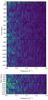 |
Fig. 5 Short-time Fourier transforms of the Kepler light curves in mask 45 (upper) and 32 (lower) for all observed quarters for a 30-day time window and progressing in the time series with a step of 3 days, zoomed into the region of low-frequency amplitude excess. Brighter colours represent higher amplitudes. |
No obvious connection between the quasi-periodicities in the photosphere and in the wind was found for HD 188209 so far. However, all the data sets available in the literature have too few spectra, too sparse sampling, and too limited time base to find periodicities with appropriate precision. Given the limited amount of spectra, all these studies only considered the variability inside the line profile, without performing frequency analysis, by means of the so-called temporal variance spectrum (Fullerton et al. 1996). This quantity is very useful to estimate the overall level of variability that is present in a small series of spectral lines assembled with sparse sampling. Its capacity to unravel the cause of this variability is limited. Here, we focus on the temporal line variability in a large data set of spectra with a long time base with the aim to investigate the physical reasons of its origin. We do this by considering specialised line-profile quantities that are specifically designed to allow for time-series analysis without being affected by uncertainties due to spectrum normalisation, as is discussed below.
We take a major step ahead compared to the spectroscopy results in the literature from new extensive long-term spectroscopic time series assembled with the following four instruments:
-
The fiber-fed HERMES échelle spectrograph attached to the1.2 m Mercator telescope at Roque de losMuchachos, Island of La Palma, Spain, operatedin the high-resolution (R = 85 000) mode (Raskin et al. 2011).
-
The high-resolution FIbre-fed Échelle Spectrograph (FIES) attached to the Nordic Optical Telescope (NOT) at Roque de los Muchachos, Island of La Palma, Spain, operated in the high-resolution (R = 46 000) mode (Telting et al. 2014).
-
The T13 2.0 m Automatic Spectroscopic Telescope (AST) with the fiber-fed cross-dispersed échelle spectrograph in the resolution mode of R = 30 000 operated at the Fairborn Observatory, USA. A full description of the instrument and data reducation pipeline is available in Eaton & Williamson (2004).
-
The prototype SONG node échelle spectrograph, operational at Observatory del Teide on Tenerife, Spain (Grundahl et al. 2007; Uytterhoeven et al. 2012; Grundahl et al. 2017). The SONG observations of HD 188209 were obtained in ThAr mode with slit 5 and have R = 77 000.
A summary of the characteristics of all the data sets analysed in this paper is given in Table 2.
Summary of the observations treated in this work; N is the total number of measurements and ΔT is the total time base.
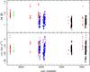 |
Fig. 6 Centroid velocity (lower panel) and equivalent width (upper panel) of the entire spectroscopic data set for the He i 5875 Å line, according to the following colour code: red = HERMES, green = FIES, blue = AST, and black = SONG. |
These four instruments were constructed with different purposes and are attached to telescopes of different sizes. The specific aim of HERMES is to obtain maximal capacity to detect time-resolved line-profile variability such that the S/N is important. The FIES is a similar spectrograph but delivers lower resolution and its temperature is less well stabilised. The main goal of SONG is to gain maximum precision in radial-velocity variations by means of an iodine cell for solar-like oscillation studies (Grundahl et al. 2017), but it also offers a ThAr option, which we used here. As we show below (see Figs. 7 and 8) the lower resolving power of AST combined with the lower S/N it delivers imply that these data are at the limit of what we need to properly detect and interpret the variability of HD 188209. But adding this data set gave compatible results so we kept them in the analysis and adopted an approach taking the S/N into account. Indeed, the S/N levels achieved with the four instruments are different for similar integration times and provide us with a way to properly weigh the data when intepreting the variability.
In the following, we focus mainly on those spectral lines that are available for the four independent spectroscopic data sets listed in Table 2 and do not suffer from order merging uncertainties in their line wings. This is the case for nine spectral lines. We also considered the Si iii 4567 Å line for its strong diagnostic power of stellar oscillations (Aerts et al. 2004) and of surface spots (Briquet et al. 2004) of hot stars, although it is not available in all data sets. In addition, even though it is only available in the HERMES data owing to order merging for the other three instruments that is too poor, we considered Hγ an important diagnostic of the gravity behaviour of the star.
For each spectral line, we computed its line moments as good diagnostics for variability by adopting their definition by Aerts et al. (1992). It is crucial to define the optimal integration limits in the line wings when computing the moments for the detection and interpretation of low-amplitude line-profile variability (e.g. Chapters 5 and 6 in Aerts et al. 2010 and Zima 2008, for extensive descriptions and publicly available software). Since we aim to merge the moments of the same spectral lines obtained with four different instruments, we determined the most optimal integration limits per line by careful visual inspection after overplotting the entire time series. In this paper, we concentrate on the equivalent width of the lines (the moment of order zero, hereafter abbreviated as EW) and on their heliocentric centroid velocity (the first-order moment, denoted as ⟨ v ⟩). Typical uncertainties for the centroid velocities due to uncertainties in the integration limits and the noise in the spectral line range from 0.1 to 0.4 km s-1, while the systematic uncertainty due to limited knowledge of the laboratory wavelength can reach up to a few km s-1. The latter is not of importance when studying time variability of one and the same particular spectral line. The systematic uncertainty is only of importance when comparing the average value of the centroid velocity for different spectral lines to interpret their amplitude as a function of the formation depth in the stellar photosphere or wind.
The atomic data are not equally good for different spectral lines. In view of this, it is highly advantageous to make a line-by-line analysis per instrument and combine the line diagnostic values in Fourier domain rather than in the time domain. Indeed, merging in the time domain suffers from slight inconsistencies in Doppler velocities derived from adopted laboratory wavelengths for various lines and from imperfections in the normalisation of the continuum flux, while merging in the Fourier domain is not affected by that. Such an approach also allows us to combine the temporal variability from entirely different quantities derived from photometry and spectroscopy and gives us the opportunity to reveal low-amplitude variations that appear consistently in different types of independent data, but each of these variations, separately, have a S/N that is too low to be significant.
The method of combining data in the Fourier domain was already applied and illustrated by Aerts et al. (2006) to discover previously unknown low-amplitude non-radial oscillation modes in the archetype monoperiodic βCep star δCeti from the combination of MOST space photometry and high-resolution spectroscopy. The rationale behind it is that the discrete Fourier transforms of different time series data of the same variable star all achieve a maximum at frequencies that are present in the data, while spurious frequencies due to noise or aliasing are different for the various independent data sets. In this respect, it is particularly useful to combine data sets with a different sampling rate, as is the case for the SONG and HERMES data. Multiplication of the Fourier transforms of the different data sets, after normalising them according to the frequency of maximal amplitude, implies that true frequencies get higher multiplied dimensionless amplitude while spurious frequencies tend to cancel each other. In the case of δCeti mentioned above, it concerned frequencies of standing waves due to coherent heat-driven oscillation modes. However, the same principle also applies to isolated frequencies of standing waves excited stochastically as in sun-like stars and red giants, or to frequencies belonging to an entire spectrum of travelling waves. Whatever their excitation mechanism, standing waves or travelling waves inside a star have frequency values that are connected with the stellar structure properties and so they occur at the same values in the various data sets.
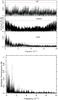 |
Fig. 7 Amplitude spectra for the EW of the He i 5875 Å line for the three individual spectrographs with sufficient data. In the upper panels, the red dashed lines indicate four times the average noise level computed over the range [0,10] d-1. The lower panel shows the result of multiplying the periodograms in the upper panels after weighing them according to the S/N of the dominant frequency and placing the dominant frequency after this multiplication at value 1. |
4.1. Showcase of the He I 5875 Å line
We first considered the He i 5875 Å to illustrate the variability behaviour as this line leads to the highest significance for the variability in terms of S/N in the line diagnostics in the four spectroscopic data sets. The individual zeroth and first moment variations of the He i 5875 Å line are shown in Fig. 6. It can be seen that slight differences occur in the EW of the line for the four spectrographs but also for the same spectrograph during different epochs. This may in part be due to imperfect normalisation, but it may also be caused by the rather irregular variability of the star, as revealed in the Kepler data in Fig. 3. Even though the moments in the definition by Aerts et al. (1992) are specifically defined such as to compensate optimally for small differences in the EW (cf. lower panel of Fig. 6), it is advantageous to treat the four ⟨ v ⟩ data sets separately, given that the four average values of this quantity per spectrograph are not equal and merging in the time domain prior to the computation of the Fourier transform would introduce spurious low frequencies.
The individual Scargle periodograms (Scargle 1982) for the HERMES, SONG, and AST data sets of the EW and ⟨ v ⟩ of the He i 5875 Å line are shown in the upper three panels of Figs. 7 and 8 (the FIES data set being too scarce for this purpose). As anticipated, these periodograms suffer from daily aliasing, a well-known phenomenon in time-series analysis of single-site data sets. The ⟨ v ⟩ based on the AST data do not lead to significant frequencies (maximum amplitude typically between 3 and 4 times the S/N), but the HERMES and SONG data sets reveal significant low-frequency amplitude with a factor typically between 10 to 12 times the S/N for SONG and 4 to 6 times the S/N for HERMES (Fig. 8). For the EW, the significance levels are typically somewhat lower than for the ⟨ v ⟩ (Fig. 7).
For each of these individual periodograms, the maximum amplitude was sought and transformed to its value expressed as a function of the average S/N, where the latter was computed in the Scargle periodogram over the frequency range [10,20] d-1. The dashed lines in Figs. 7 and 8 are placed at four times this S/N. Subsequently, the three Scargle periodograms expressed in units of the S/N were multiplied, after which they were normalised such that the maximum peak after this multiplication was placed at value 1.0. The results of this procedure are shown in the lower panels of Figs. 7 and 8. It can be seen that this procedure leads to a far clearer view of the variability in this single spectral line, as the aliasing and noise peaks in the individual three data sets are substantially reduced in this way. Variability is found to occur at a multitude of low frequencies, in the range [0,2] d-1, entirely in agreement with the Kepler scattered-light photometry.
The morphology of the normalised periodogram in Fig. 8 is unlike those encountered for B dwarfs pulsating multiperiodically in coherent heat-driven gravity modes (e.g. De Cat & Aerts 2002). In view of this discrepancy and the similar amplitude spectrum obtained from the Kepler photometry, we compare the frequency spectrum of HD 188209 in Fig. 8 with predictions from hydrodynamical simulations based on convectively driven internal gravity waves. In order to do so, we follow a similar approach as in Aerts & Rogers (2015); our case is simpler because the 2D simulations by Rogers et al. (2013) provide us with velocity information that allows a direct meaningful comparison with Fig. 8, while Aerts & Rogers (2015) had to transform this information to brightness variations to be able to compare with CoRoT light curves. Given that HD 188209 is evolved and about ten times more massive than the model of 3 M⊙ adopted for the simulations by Rogers et al. (2013), we performed a scaling with a factor 0.53 that occurs between the frequencies of dipole gravity waves of a 3 M⊙ ZAMS star and of a 30 M⊙ TAMS star (Shiode et al. 2013, Table 1). Moreover, we normalise the tangential velocity of the 2D simulations, where the radial component is entirely negligible (see Fig. 1 in Aerts & Rogers 2015, right panel), to their highest amplitude, considering simulation run D11 (a non-rigidly rotating star whose core rotates 1.5 times faster than its envelope). The outcome is presented in Fig. 9. While this exercise does not allow a peak-to-peak comparison of the frequencies in the two spectra, the overall morphology in Figs. 8 and 9 is similar.
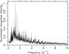 |
Fig. 9 Normalised periodogram for the tangential velocity of internal gravity waves occurring in 2D simulation D11 in Rogers et al. (2013), properly scaled in frequency to take into account the mass and evolutionary status of HD 188209 with respect to the simulated stellar model. |
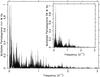 |
Fig. 10 Multiplied Scargle periodograms after weighting according to the S/N of the frequency with highest amplitude for the ⟨ v ⟩ (and EW in the inset) of the He i 5875 Å line and Kepler photometry in mask 32. |
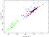 |
Fig. 11 Centroid velocities based on different spectral lines available in the HERMES spectroscopy: black: He ii 4541 Å versus He ii 5410 Å; red: He i 5015 Å versus He i 4922 Å; blue: He i 5875 Å versus Si iii 4567 Å; green: Hβ versus Hγ. |
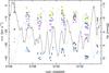 |
Fig. 12 Centroid velocity (left y-axis) and Kepler photometry in mask 45 (right y-axis) during the only epoch where the space and ground-based data overlap in time. The colour coding is as follows: Hβ: black; Hγ: light blue; He i 4713 Å: dark blue; He i 4922 Å: cyan; He i 5015 Å: pink; He i 5875 Å: grey; He ii 4541 Å: green; He ii 5410 Å: yellow; C iv 5812 Å: orange; Si iii 4567 Å: purple. To guide the eye, the observed Kepler light curve is shown as dotted line while its mirrored version with respect to the average Kepler magnitude is shown as the full line. |
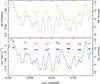 |
Fig. 13 Centroid velocity (left y-axis, bottom panel) and Hα emission strength expressed in continuum units (left y-axis, top panel) and the Kepler photometry in mask 45 (right y-axes) during the only epoch where the space and ground-based data overlap in time. The colour coding is as follows: Hα: light green; Hβ: black; Hγ: light blue; He i 4686 Å: red. To guide the eye, the observed Kepler light curve is shown as dotted line while its mirrored version with respect to the average Kepler magnitude is shown as the full line. |
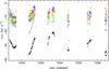 |
Fig. 14 Excerpt of the SONG spectroscopy during 5 consecutive days. The centroid velocity is shown for 9 available spectral lines; the He ii 4686 Å line was avoided for visibility purposes. The colour coding is the same as in Fig. 12. |
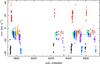 |
Fig. 15 HERMES spectroscopy of HD 188209 covering some 870 days of monitoring during four epochs. The centroid velocity is shown for all available spectral lines except Hα. The colour coding is the same as in Fig. 12. For visibility purposes, the values for each spectral line were shifted in time with multiples of 12 d, Hβ in black representing the true HJD. |
Next, we went one step further and considered a multiplied Scargle periodogram deduced from the three spectroscopic He i 5875 Å data sets and the Kepler data in mask 32 as a fourth independent data set. Its highest amplitude peak has a significance of 137 times the S/N in the frequency range [10,20] d-1, because the average S/N is 27 ppm in that interval. The outcome of this multiplication is shown in Fig. 10. Figures 7, 8, and 10 all point towards the same conclusion: HD 188209 reveals significant variability with an entire spectrum of significant frequencies below 2 d-1. The morphology in the periodograms point towards travelling waves at the origin of this variability, given the density of frequency peaks and the absence of any clear relationship between the dominant peaks. Thus, we find fully compatible variability results between the Kepler scattered-light space photometry and the He i 5875 Å spectral line, both when treating these data separately and in a combined analysis.
4.2. Other spectral lines
We repeated the entire procedure described in the previous section for the other photospheric lines that are present in all four spectroscopic data sets. It concerns He i 4713 Å, He i 4922 Å, He i 5015 Å, He ii 4541 Å, He ii 5410 Å, C iv 5812 Å. Moreover, we considered the Si iii 4567 Å line in the HERMES spectra. All these lines behave fully consistently with the He i 5875 Å line in terms of time-variability patterns and morphology of the separate and multiplied Fourier transforms, where the only difference is the amplitudes of their EW and ⟨ v ⟩ time series (not the relative amplitudes expressed in terms of the S/N, which are remarkable similar for all those lines). Figure 11 shows a comparison of the ⟨ v ⟩-values for several lines available in the HERMES spectroscopy, where we plot them line-by-line. It can be seen that there is large consistency among the values of the centroid velocities. The values of ⟨ v ⟩ for the He i lines have the strongest similarity. The Si iii 4567 Å line is more affected by the base of the wind than the He i 5875 Å line and the Balmer lines are clearly formed further out in the wind than the helium and metal lines.
Next, we considered two lines available in all four data sets but formed partially in the wind and in the photosphere, i.e. Hβ and He ii 4686 Å. The latter spectral line shows an unexplained global shift to the red with an average velocity value of about +45 km s-1 with respect to all other spectral lines when considering its laboratory wavelength of 4685.71 Å. This anomaly occurs for all four of the spectroscopic data sets. It is known that the He ii 4686 Å line is partially formed in the stellar wind (e.g. Massey et al. 2004; Martins et al. 2015b). As such, its formation is affected by the temperature, wind density, metallicity, and amount of EUV flux. However, we cannot explain the detected redward shift corresponding with some 0.7 Å which we find for the absorption profile of this line. We are aware of at least one other star where this line is in absorption and for which the same anomaly is reported in the literature (see Fig. 15 in Massey et al. 2004, for the O8.5 I(f) supergiant AV 469 in the Small Magellanic Cloud, a star with quite similar fundamental parameters than HD 188209 except for the metallicity). Recent laboratory measurements of He ii pointed out that its spectral line structure near 4686 Å is complex (Syed et al. 2012). It seems prudent to observe caution in its interpretation concerning absorption lines of hot evolved stars.
The Hβ line of HD 188209 behaves very similarly to the Hγ line, where the latter is only suitable for our analysis in the HERMES data set. This is also the case for the Hα and Si iii 4567 Å lines, which we only considered in the HERMES data set. Apart from the global shift of its average centroid velocity with respect to the other lines, the variability behaviour of the He ii 4686 Å line is fully consistent with that of the other spectral lines and confirms that this line is partially formed in the wind.
Unfortunately, there is only one short period spanning eight days for which we have both Kepler space photometry and ground-based spectroscopy. It concerns data in mask 45 and HERMES spectroscopy. The centroid velocities of all the available spectral lines and the space photometry taken during these eight days are shown in Fig. 12. The He ii 4686 Å line and Hα fall outside the boundaries of this plot. It is seen that all spectral lines show consistent behaviour in their centroid velocity in the time domain.
The He ii 4686 Å line is shown along with Hα, Hβ, and Hγ, and in comparison with the Kepler photometry, in Fig. 13. It can be seen that He ii 4686 Å, Hβ, and Hγ are fully in agreement with each other in terms of variability. The Hα emission varies in antiphase with the Hα centroid velocity. While the relation between the spectroscopic variability and the Kepler photometry is hard to unravel from Figs. 12 and 13, the morphology of the various quantities in the time domain is similar. The spectroscopic variability of the wind and of the photosphere, and the photometric variability are all in agreement in terms of amplitudes and periodicities.
4.3. Summary of variability of the centroid velocities
Among the spectroscopic data sets, the highest sampling rate is obtained with SONG. A 5 d excerpt of ⟨ v ⟩ derived from nine spectral lines available in these data is shown in Fig. 14. We find similar behaviour for most of the spectral lines. The figure reveals different behaviour in variability from night to night with dominant periodicities that are typically longer than 10 h and quite different amplitudes per night. This confirms the earlier finding of variability with frequencies below 2 d-1 in the Fourier domain, but now by visual inspection in the time domain based on the spectral lines available in the SONG spectroscopy.
Thanks to its construction, the HERMES spectrograph offers the best long-term stability of the four instruments used here. Indeed, its fiber-fed design connected with a temperature-controlled room and its dedicated calibration pipeline were specifically defined and implemented with long-term monitoring of variable phenomena in mind (Raskin et al. 2011). This data set of HD 188209 is therefore best suited to illustrate the long-term spectroscopic variability of the star in the time domain. We show the centroid velocities for the 11 available spectral lines in the HERMES data for the first four epochs of monitoring in Fig. 15, where the HJD for the various spectral lines are shifted along the x-axis of the plot with multiples of 12 days for visibility purposes. The data for the first epoch in Fig. 15 corresponds with that shown in Fig. 12. Figures 12 and 15 illustrate the consistency between the ⟨ v ⟩-values for the various spectral lines, both on a timescale of a week and two years.
A summary of all the computed line diagnostics is provided in Table 3 for the HERMES data for which the centroid velocities are plotted in Fig. 15 (except for Hα as these do not fit the plot). The colour coding adopted in Figs. 12–15 is indicated and the lines are listed in order of increasing average centroid velocity, corresponding to increasing line-formation depth into the wind/photosphere. Despite unknown systematic uncertainties for ⟨ v ⟩ owing to limitations in the knowledge of the laboratory wavelengths (of order km s-1), we detect a radial gradient in the average centroid velocities for the different lines (Table 3), where, as already mentioned, the He ii 4686 Å line behaves anomalously (as also shown in Fig. 15). The peak-to-peak variability of ⟨ v ⟩ is very similar if one keeps in mind that line blending affects this range and is different for the various spectral lines. Even though they are formed partly in the wind in view of their more negative average velocity, the variability of Hβ and Hγ behaves similarly to those the helium and metal lines. Hence, the photospheric variability does not change at the bottom of the stellar wind. Only the Hα variability seems dominated by the wind behaviour.
Summary of variability properties of the centroid velocity ⟨ v ⟩ and EW for 12 spectral lines of HD 188209 available in the HERMES data, spanning 1800 d.
5. Discussion and conclusions
In this work, we used the Kepler spacecraft far beyond its nominal performance by studying scattered-light photometry of the bright blue supergiant HD 188209 while it was situated in between active CCDs. Aperture photometry of its scattered light delivered the first four-year long uninterrupted high-cadence light curve of a blue supergiant, reaching a precision of some 27 ppm at frequencies above 10 d-1. We found similarities in the morphology of the frequency spectrum derived from the scattered light and from line-profile diagnostics of several spectral lines in long-term ground-based high-resolution spectroscopy. A major conclusion of this work is that the range of detected frequencies in the space photometry and ground-based spectroscopy is the same. All the frequency spectra point towards variability occurring in the photosphere and consistently propagating into the bottom of the stellar wind. The nature of the short-time Fourier transforms of the high-cadence photometry excludes an interpretation in terms of standing waves connected with non-radial gravity-mode oscillations, but rather points towards the excitation of an entire spectrum of travelling internal gravity waves triggered by core and/or envelope convection. This is a plausible explanation in terms of the measured velocity amplitudes and the multitude of detected frequencies in the regime below 2 d-1.
While we could not find a simple point-to-point relationship between the photometric and spectroscopic data that were taken simultaneously, we did find full consistency in the frequency range caused by these independent data sets. Moreover, there are similarities in the overall morphologies of the variable patterns in the time domain and frequency spectra in Fourier space derived from the scattered-light photometry and centroid velocities deduced from the spectroscopy. The observed frequency spectra of HD 188209 are in qualitative agreement with those for the tangential velocities based on 2D hydrodynamical simulations of internal gravity waves in a massive star. We thus conclude to have found the first observational evidence of the occurrence of such waves in a massive blue supergiant. Along with the discovery of such waves in young O-type dwarfs (Blomme et al. 2011; Aerts & Rogers 2015), we revealed at least one important mechanism of angular momentum transport active in massive stars during and beyond core-hydrogen burning that is currently not included in stellar evolution models. It remains to be studied how much impact the omission of this ingredient has on stellar evolution theory.
The tangential velocities associated with internal gravity waves in the stellar photosphere of massive stars are of order a tenth of a km s-1 per individual wave (Rogers et al. 2013). It has already been shown by Aerts & Rogers (2015, their Fig. 5) that the collective effect of hundreds of such internal gravity waves on line profiles is very similar to the effect due to a collection of coherent heat-driven gravity-mode oscillations, particularly for the line wings. Given that both coherent standing gravity-mode oscillations and running gravity waves have completely dominant tangential velocities (at the level that their radial velocity component is negligible), any proper modelling of macroturbulent line broadening due to gravity waves as detected in HD 188209 requires fitting a tangential macroturbulent velocity field to the spectral lines.
Acknowledgments
This project has received funding from the European Research Council (ERC) under the European Union’s Horizon 2020 research and innovation programme (Advanced Grant agreements No. 670519: MAMSIE “Mixing and Angular Momentum tranSport in MassIvE stars” and No. 267864: ASTERISK “ASTERoseismic Investigations with SONG and Kepler”). Funding for the Stellar Astrophysics Centre is provided by The Danish National Research Foundation (Grant DNRF106). P.I.P. acknowledges support from The Research Foundation Flanders (FWO), Belgium and E.M. was supported by the People Programme (Marie Curie Actions) of the European Union’s Seventh Framework Programme FP7/2007-2013/ under REA grant agreement No. 623303 (ASAMBA). The authors are grateful to P. Beck, G. Holgado, S. Rodriguez, V. Schmid, and C. Gonzalez for having taken a few additional spectra included in this study. Funding for the Kepler Discovery mission was provided by NASA’s Science Mission Directorate. The authors gratefully acknowledge the entire Kepler team, whose outstanding efforts have made these results possible. This research has made use of the SIMBAD database, operated at CDS, Strasbourg, France, and of the Multimission Archive at STScI (MAST), USA. We also acknowledge use of the Atomic Line List offered by the University of Kentucky, USA and maintained by Peter van Hoof, Royal Observatory of Belgium.
References
- Aerts, C. 2015, Astron. Nachr., 336, 477 [NASA ADS] [CrossRef] [Google Scholar]
- Aerts, C., & Rogers, T. M. 2015, ApJ, 806, L33 [NASA ADS] [CrossRef] [Google Scholar]
- Aerts, C., de Pauw, M., & Waelkens, C. 1992, A&A, 266, 294 [NASA ADS] [Google Scholar]
- Aerts, C., De Cat, P., Handler, G., et al. 2004, MNRAS, 347, 463 [NASA ADS] [CrossRef] [Google Scholar]
- Aerts, C., Marchenko, S. V., Matthews, J. M., et al. 2006, ApJ, 642, 470 [NASA ADS] [CrossRef] [Google Scholar]
- Aerts, C., Lefever, K., Baglin, A., et al. 2010, A&A, 513, L11 [NASA ADS] [CrossRef] [EDP Sciences] [Google Scholar]
- Aerts, C., Simón-Díaz, S., Catala, C., et al. 2013, A&A, 557, A114 [NASA ADS] [CrossRef] [EDP Sciences] [Google Scholar]
- Bedding, T. R., Mosser, B., Huber, D., et al. 2011, Nature, 471, 608 [NASA ADS] [CrossRef] [PubMed] [Google Scholar]
- Bischoff-Kim, A., & Østensen, R. H. 2011, ApJ, 742, L16 [NASA ADS] [CrossRef] [Google Scholar]
- Blomme, R., Mahy, L., Catala, C., et al. 2011, A&A, 533, A4 [NASA ADS] [CrossRef] [EDP Sciences] [Google Scholar]
- Briquet, M., Aerts, C., Lüftinger, T., et al. 2004, A&A, 413, 273 [NASA ADS] [CrossRef] [EDP Sciences] [Google Scholar]
- Buysschaert, B., Aerts, C., Bloemen, S., et al. 2015, MNRAS, 453, 89 [NASA ADS] [CrossRef] [Google Scholar]
- Chaplin, W. J., & Miglio, A. 2013, ARA&A, 51, 353 [NASA ADS] [CrossRef] [Google Scholar]
- Charpinet, S., Van Grootel, V., Brassard, P., et al. 2014, in 6th Meeting on Hot Subdwarf Stars and Related Objects, eds. V. van Grootel, E. Green, G. Fontaine, & S. Charpinet, ASP Conf. Ser., 481, 105 [Google Scholar]
- De Cat, P., & Aerts, C. 2002, A&A, 393, 965 [NASA ADS] [CrossRef] [EDP Sciences] [Google Scholar]
- Degroote, P., Aerts, C., Baglin, A., et al. 2010, Nature, 464, 259 [NASA ADS] [CrossRef] [PubMed] [Google Scholar]
- Degroote, P., Aerts, C., Michel, E., et al. 2012, A&A, 542, A88 [NASA ADS] [CrossRef] [EDP Sciences] [Google Scholar]
- Deheuvels, S., Ballot, J., Beck, P. G., et al. 2015, A&A, 580, A96 [NASA ADS] [CrossRef] [EDP Sciences] [Google Scholar]
- Eaton, J. A., & Williamson, M. H. 2004, Astron. Nachr., 325, 522 [NASA ADS] [CrossRef] [Google Scholar]
- Fossati, L., Schneider, F. R. N., Castro, N., et al. 2016, A&A, 592, A84 [NASA ADS] [CrossRef] [EDP Sciences] [Google Scholar]
- Foster, H. M., Reed, M. D., Telting, J. H., Østensen, R. H., & Baran, A. S. 2015, ApJ, 805, 94 [NASA ADS] [CrossRef] [Google Scholar]
- Fullerton, A. W., Gies, D. R., & Bolton, C. T. 1996, ApJS, 103, 475 [NASA ADS] [CrossRef] [Google Scholar]
- Fullerton, A. W., Massa, D. L., & Prinja, R. K. 2006, ApJ, 637, 1025 [NASA ADS] [CrossRef] [Google Scholar]
- Grundahl, F., Kjeldsen, H., Christensen-Dalsgaard, J., Arentoft, T., & Frandsen, S. 2007, Commun. Asteroseismol., 150, 300 [NASA ADS] [CrossRef] [Google Scholar]
- Grundahl, F., Fredslund Andersen, M., Christensen-Dalsgaard, J., et al. 2017, ApJ, 836, 142 [NASA ADS] [CrossRef] [Google Scholar]
- Grunhut, J. H., Wade, G. A., Neiner, C., et al. 2017, MNRAS, 465, 2432 [NASA ADS] [CrossRef] [Google Scholar]
- Guzik, J. A., Houdek, G., Chaplin, W. J., et al. 2016, ApJ, 831, 17 [NASA ADS] [CrossRef] [Google Scholar]
- Hekker, S., & Christensen-Dalsgaard, J. 2016, A&ARv, submitted [arXiv:1609.07487] [Google Scholar]
- Israelian, G., Herrero, A., Musaev, F., et al. 2000, MNRAS, 316, 407 [NASA ADS] [CrossRef] [Google Scholar]
- Kaper, L., Henrichs, H. F., Nichols, J. S., et al. 1996, A&AS, 116, 257 [NASA ADS] [CrossRef] [EDP Sciences] [Google Scholar]
- Koch, D. G., Borucki, W. J., Basri, G., et al. 2010, ApJ, 713, L79 [NASA ADS] [CrossRef] [Google Scholar]
- Kolenberg, K., Bryson, S., Szabó, R., et al. 2011, MNRAS, 411, 878 [NASA ADS] [CrossRef] [Google Scholar]
- Kurtz, D. W., Saio, H., Takata, M., et al. 2014, MNRAS, 444, 102 [NASA ADS] [CrossRef] [Google Scholar]
- Lesh, J. R. 1968, ApJS, 17, 371 [NASA ADS] [CrossRef] [EDP Sciences] [Google Scholar]
- Maíz Apellániz, J., Alfaro, E. J., Arias, J. I., et al. 2015, in Highlights of Spanish Astrophysics VIII, eds. A. J. Cenarro, F. Figueras, C. Hernández-Monteagudo, J. Trujillo Bueno, & L. Valdivielso, 603 [Google Scholar]
- Markova, N., Puls, J., Scuderi, S., & Markov, H. 2005, A&A, 440, 1133 [NASA ADS] [CrossRef] [EDP Sciences] [Google Scholar]
- Martins, F., & Palacios, A. 2013, A&A, 560, A16 [NASA ADS] [CrossRef] [EDP Sciences] [Google Scholar]
- Martins, F., Hervé, A., Bouret, J.-C., et al. 2015a, A&A, 575, A34 [NASA ADS] [CrossRef] [EDP Sciences] [Google Scholar]
- Martins, F., Marcolino, W., Hillier, D. J., Donati, J.-F., & Bouret, J.-C. 2015b, A&A, 574, A142 [NASA ADS] [CrossRef] [EDP Sciences] [Google Scholar]
- Massey, P., Bresolin, F., Kudritzki, R. P., Puls, J., & Pauldrach, A. W. A. 2004, ApJ, 608, 1001 [Google Scholar]
- Metcalfe, T. S., Chaplin, W. J., Appourchaux, T., et al. 2012, ApJ, 748, L10 [NASA ADS] [CrossRef] [Google Scholar]
- Moravveji, E., Guinan, E. F., Shultz, M., Williamson, M. H., & Moya, A. 2012, ApJ, 747, 108 [NASA ADS] [CrossRef] [Google Scholar]
- Moravveji, E., Aerts, C., Pápics, P. I., Triana, S. A., & Vandoren, B. 2015, A&A, 580, A27 [NASA ADS] [CrossRef] [EDP Sciences] [Google Scholar]
- Moravveji, E., Townsend, R. H. D., Aerts, C., & Mathis, S. 2016, ApJ, 823, 130 [NASA ADS] [CrossRef] [MathSciNet] [Google Scholar]
- Murphy, S. J., Fossati, L., Bedding, T. R., et al. 2016, MNRAS, 459, 1201 [NASA ADS] [CrossRef] [Google Scholar]
- Pápics, P. I., Moravveji, E., Aerts, C., et al. 2014, A&A, 570, A8 [NASA ADS] [CrossRef] [EDP Sciences] [Google Scholar]
- Pápics, P. I., Tkachenko, A., Aerts, C., et al. 2015, ApJ, 803, L25 [Google Scholar]
- Pápics, P. I., Tkachenko, A., Van Reeth, T., et al. 2017, A&A, 598, A74 [NASA ADS] [CrossRef] [EDP Sciences] [Google Scholar]
- Pope, B. J. S., White, T. R., Huber, D., et al. 2016, MNRAS, 455, L36 [NASA ADS] [CrossRef] [Google Scholar]
- Raskin, G., van Winckel, H., Hensberge, H., et al. 2011, A&A, 526, A69 [NASA ADS] [CrossRef] [EDP Sciences] [Google Scholar]
- Rogers, T. M., Lin, D. N. C., McElwaine, J. N., & Lau, H. H. B. 2013, ApJ, 772, 21 [NASA ADS] [CrossRef] [Google Scholar]
- Saio, H., Kuschnig, R., Gautschy, A., et al. 2006, ApJ, 650, 1111 [NASA ADS] [CrossRef] [Google Scholar]
- Saio, H., Kurtz, D. W., Takata, M., et al. 2015, MNRAS, 447, 3264 [NASA ADS] [CrossRef] [Google Scholar]
- Sana, H., de Mink, S. E., de Koter, A., et al. 2012, Science, 337, 444 [Google Scholar]
- Scargle, J. D. 1982, ApJ, 263, 835 [NASA ADS] [CrossRef] [Google Scholar]
- Schmid, V. S., & Aerts, C. 2016, A&A, 592, A116 [NASA ADS] [CrossRef] [EDP Sciences] [Google Scholar]
- Shiode, J. H., Quataert, E., Cantiello, M., & Bildsten, L. 2013, MNRAS, 430, 1736 [NASA ADS] [CrossRef] [Google Scholar]
- Simón-Díaz, S., & Herrero, A. 2014, A&A, 562, A135 [NASA ADS] [CrossRef] [EDP Sciences] [Google Scholar]
- Simón-Díaz, S., Negueruela, I., Maíz Apellániz, J., et al. 2015, in Highlights of Spanish Astrophysics VIII, eds. A. J. Cenarro, F. Figueras, C. Hernández-Monteagudo, J. Trujillo Bueno, & L. Valdivielso, 576 [Google Scholar]
- Simón-Díaz, S., Godart, M., Castro, N., et al. 2017, A&A, 597, A22 [NASA ADS] [CrossRef] [EDP Sciences] [Google Scholar]
- Sota, A., Maíz Apellániz, J., Walborn, N. R., et al. 2011, ApJS, 193, 24 [NASA ADS] [CrossRef] [Google Scholar]
- Syed, W. A. A., Shah, N. A., & Wazir, S. 2012, Science and Technology, 2, 122 [NASA ADS] [CrossRef] [Google Scholar]
- Telting, J. H., Avila, G., Buchhave, L., et al. 2014, Astron. Nachr., 335, 41 [NASA ADS] [CrossRef] [Google Scholar]
- Tkachenko, A., Aerts, C., Pavlovski, K., et al. 2012, MNRAS, 424, L21 [NASA ADS] [Google Scholar]
- Tkachenko, A., Aerts, C., Yakushechkin, A., et al. 2013, A&A, 556, A52 [NASA ADS] [CrossRef] [EDP Sciences] [Google Scholar]
- Tkachenko, A., Degroote, P., Aerts, C., et al. 2014, MNRAS, 438, 3093 [NASA ADS] [CrossRef] [Google Scholar]
- Triana, S. A., Moravveji, E., Pápics, P. I., et al. 2015, ApJ, 810, 16 [NASA ADS] [CrossRef] [Google Scholar]
- Uytterhoeven, K., Pallé, P. L., Grundahl, F., et al. 2012, Astron. Nachr., 333, 1103 [NASA ADS] [CrossRef] [Google Scholar]
- Van Reeth, T., Tkachenko, A., & Aerts, C. 2016, A&A, 593, A120 [NASA ADS] [CrossRef] [EDP Sciences] [Google Scholar]
- Walborn, N. R. 1972, AJ, 77, 312 [NASA ADS] [CrossRef] [Google Scholar]
- Walborn, N. R., & Fitzpatrick, E. L. 1990, PASP, 102, 379 [NASA ADS] [CrossRef] [Google Scholar]
- White, T. R., Pope, B. J. S., Antoci, V., et al. 2017, MNRAS, submitted [Google Scholar]
- Zima, W. 2008, Commun. Asteroseismol., 157, 387 [NASA ADS] [Google Scholar]
All Tables
Spectroscopically derived properties of HD 188209 reported in the recent literature based on a non-LTE analysis.
Summary of the observations treated in this work; N is the total number of measurements and ΔT is the total time base.
Summary of variability properties of the centroid velocity ⟨ v ⟩ and EW for 12 spectral lines of HD 188209 available in the HERMES data, spanning 1800 d.
All Figures
|
Fig. 1 Position of the two apertures (45: left), 32 (right) in the Kepler FoV capturing the scattered light of HD 188209 (situated in the black band above the red cross in between active silicon). |
| In the text | |
|
Fig. 2 Example of pixel masks used to create three versions of the light curves for star 45 (left) and 32 (right). The detected light curve is plotted within each pixel and represents an addition of 270 individual exposures of 6.54 s, added on board of the satellite. In long-cadence mode, such pixel data are downloaded from the spacecraft in time stamps of 29.42 min. The values listed in every pixel indicate the S/N level of the flux in the pixel. The red dots in the pixels with green and blue borders were used to extract the standard Kepler light curves. We also computed light curves based on the data in the yellow pixels alone and from adding the green, blue, and yellow pixels. |
| In the text | |
|
Fig. 3 Light curves in masks 32 (grey circles) and 45 (black circles) covering the full length (upper), quarters 4 and 5 (middle) and a zoom of 20 d. |
| In the text | |
|
Fig. 4 Amplitude spectrum for the Kepler light curves of masks 32 (grey) and 45 (black). The inset compares the spectrum of the Kepler light curve from mask 32 (grey) with the Hipparcos light curve (black) over twice the frequency range. The red dashed and blue dot-dot-dot-dashed lines indicate four times the average noise level computed over the frequency range [0,6] d-1, while the red dot-dashed line in the inset represents four times the average noise level computed over the same range [0,6] d-1 of the Hipparcos data. |
| In the text | |
|
Fig. 5 Short-time Fourier transforms of the Kepler light curves in mask 45 (upper) and 32 (lower) for all observed quarters for a 30-day time window and progressing in the time series with a step of 3 days, zoomed into the region of low-frequency amplitude excess. Brighter colours represent higher amplitudes. |
| In the text | |
|
Fig. 6 Centroid velocity (lower panel) and equivalent width (upper panel) of the entire spectroscopic data set for the He i 5875 Å line, according to the following colour code: red = HERMES, green = FIES, blue = AST, and black = SONG. |
| In the text | |
|
Fig. 7 Amplitude spectra for the EW of the He i 5875 Å line for the three individual spectrographs with sufficient data. In the upper panels, the red dashed lines indicate four times the average noise level computed over the range [0,10] d-1. The lower panel shows the result of multiplying the periodograms in the upper panels after weighing them according to the S/N of the dominant frequency and placing the dominant frequency after this multiplication at value 1. |
| In the text | |
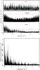 |
Fig. 8 Same as Fig. 7 but for ⟨ v ⟩ of the He i 5875 Å line. |
| In the text | |
|
Fig. 9 Normalised periodogram for the tangential velocity of internal gravity waves occurring in 2D simulation D11 in Rogers et al. (2013), properly scaled in frequency to take into account the mass and evolutionary status of HD 188209 with respect to the simulated stellar model. |
| In the text | |
|
Fig. 10 Multiplied Scargle periodograms after weighting according to the S/N of the frequency with highest amplitude for the ⟨ v ⟩ (and EW in the inset) of the He i 5875 Å line and Kepler photometry in mask 32. |
| In the text | |
|
Fig. 11 Centroid velocities based on different spectral lines available in the HERMES spectroscopy: black: He ii 4541 Å versus He ii 5410 Å; red: He i 5015 Å versus He i 4922 Å; blue: He i 5875 Å versus Si iii 4567 Å; green: Hβ versus Hγ. |
| In the text | |
|
Fig. 12 Centroid velocity (left y-axis) and Kepler photometry in mask 45 (right y-axis) during the only epoch where the space and ground-based data overlap in time. The colour coding is as follows: Hβ: black; Hγ: light blue; He i 4713 Å: dark blue; He i 4922 Å: cyan; He i 5015 Å: pink; He i 5875 Å: grey; He ii 4541 Å: green; He ii 5410 Å: yellow; C iv 5812 Å: orange; Si iii 4567 Å: purple. To guide the eye, the observed Kepler light curve is shown as dotted line while its mirrored version with respect to the average Kepler magnitude is shown as the full line. |
| In the text | |
|
Fig. 13 Centroid velocity (left y-axis, bottom panel) and Hα emission strength expressed in continuum units (left y-axis, top panel) and the Kepler photometry in mask 45 (right y-axes) during the only epoch where the space and ground-based data overlap in time. The colour coding is as follows: Hα: light green; Hβ: black; Hγ: light blue; He i 4686 Å: red. To guide the eye, the observed Kepler light curve is shown as dotted line while its mirrored version with respect to the average Kepler magnitude is shown as the full line. |
| In the text | |
|
Fig. 14 Excerpt of the SONG spectroscopy during 5 consecutive days. The centroid velocity is shown for 9 available spectral lines; the He ii 4686 Å line was avoided for visibility purposes. The colour coding is the same as in Fig. 12. |
| In the text | |
|
Fig. 15 HERMES spectroscopy of HD 188209 covering some 870 days of monitoring during four epochs. The centroid velocity is shown for all available spectral lines except Hα. The colour coding is the same as in Fig. 12. For visibility purposes, the values for each spectral line were shifted in time with multiples of 12 d, Hβ in black representing the true HJD. |
| In the text | |
Current usage metrics show cumulative count of Article Views (full-text article views including HTML views, PDF and ePub downloads, according to the available data) and Abstracts Views on Vision4Press platform.
Data correspond to usage on the plateform after 2015. The current usage metrics is available 48-96 hours after online publication and is updated daily on week days.
Initial download of the metrics may take a while.