| Issue |
A&A
Volume 602, June 2017
The VLA-COSMOS 3 GHz Large Project
|
|
|---|---|---|
| Article Number | A2 | |
| Number of page(s) | 21 | |
| Section | Catalogs and data | |
| DOI | https://doi.org/10.1051/0004-6361/201630223 | |
| Published online | 13 June 2017 | |
The VLA-COSMOS 3 GHz Large Project: Multiwavelength counterparts and the composition of the faint radio population ⋆
1 University of ZagrebPhysics Department Bijenička cesta 32 10002 Zagreb Croatia
e-mail:
[vs;ivand]@phy.hr
2 INAF–Osservatorio Astronomico di Bologna, via Gobetti 93/3, 40129 Bologna, Italy
3 Max Planck Institute for Astronomy, Königstuhl 17, 69117 Heidelberg, Germany
4 Istituto di Radioastronomia di Bologna, INAF, via P. Gobetti, 101, 40129 Bologna, Italy
5 Spitzer Science Center, California Institute of Technology, 220-6, Pasadena, CA 91125, USA
6 Harvard-Smithsonian Center for Astrophysics, 60 Garden Street, Cambridge, MA 02138, USA
7 Argelander-Institut für Astronomie, University of Bonn, Auf dem Hügel 71, 53121 Bonn, Germany
8 Aix Marseille Université, Laboratoire d’Astrophysique de Marseille, 38 rue Frédéric Joliot-Curie, 13388 Marseille, France
9 Institut d’Astrophysique de Paris, Sorbonne Universités, UPMC, Univ. Paris 06 et CNRS, UMR 7095, 98bis bd Arago, 75014 Paris, France
10 Department of Physics & Astronomy, Clemson University, Clemson, SC 29634, USA
11 Max Planck Institute for Extraterrestrial Physics, Giessenbachstr. 1, 85748 Garching, Germany
Received: 9 December 2016
Accepted: 12 April 2017
Abstract
We study the composition of the faint radio population selected from the Karl G. Jansky Very Large Array Cosmic Evolution Survey (VLA-COSMOS) 3 GHz Large Project, which is a radio continuum survey performed at 10 cm wavelength. The survey covers a 2.6 square degree area with a mean rms of ~ 2.3 μJy/beam, cataloging 10 830 sources above 5σ, and enclosing the full 2 square degree COSMOS field. By combining these radio data with optical, near-infrared (UltraVISTA), and mid-infrared (Spitzer/IRAC) data, as well as X-ray data (Chandra), we find counterparts to radio sources for ~93% of the total radio sample reaching out to z ≲ 6; these sources are found in the unmasked areas of the COSMOS field, i.e., those not affected by saturated or bright sources in the optical to near-infrared (NIR) bands. We further classify the sources as star-forming galaxies or AGN based on various criteria, such as X-ray luminosity; observed mid-infrared color; UV–far-infrared spectral energy distribution; rest-frame, near-UV optical color that is corrected for dust extinction; and radio excess relative to that expected from the star formation rate of the hosts. We separate the AGN into subsamples dominated by low-to-moderate and moderate-to-high radiative luminosity AGN, i.e., candidates for high-redshift analogs to local low- and high-excitation emission line AGN, respectively. We study the fractional contributions of these subpopulations down to radio flux levels of ~11 μJy at 3 GHz (or ~20 μJy at 1.4 GHz assuming a spectral index of –0.7). We find that the dominant fraction at 1.4 GHz flux densities above ~200 μJy is constituted of low-to-moderate radiative luminosity AGN. Below densities of ~100 μJy the fraction of star-forming galaxies increases to ~ 60%, followed by the moderate-to-high radiative luminosity AGN (~ 20%) and low-to-moderate radiative luminosity AGN (~ 20%). Based on this observational evidence, we extrapolate the fractions down to sensitivities of the Square Kilometer Array (SKA). Our estimates suggest that at the faint flux limits to be reached by the (Wide, Deep, and UltraDeep) SKA1 surveys, a selection based only on radio flux limits can provide a simple tool to efficiently identify samples highly (>75%) dominated by star-forming galaxies.
Key words: radio continuum: galaxies / catalogs
The catalog is only available at the CDS via anonymous ftp to cdsarc.u-strasbg.fr (130.79.128.5) or via http://cdsarc.u-strasbg.fr/viz-bin/qcat?J/A+A/602/A2
Visiting scientist.
© ESO, 2017
1. Introduction
Understanding how galaxies form in the early Universe and their subsequent evolution through cosmic time is a major goal of modern astrophysics. Panchromatic look-back sky surveys significantly advanced the field in the last decade, demonstrating that a multiwavelength X-ray to radio approach is key for such studies. With the major upgrades of existing radio facilities and the onset of new radio facilities, such as the Karl G. Jansky Very Large Array (VLA), Australia Telescope Compact Array (ATCA), and Atacama Large Millimeter/submillimeter Array (ALMA), which now deliver an order of magnitude increase in sensitivity, radio astronomy has entered its golden age and has moved toward the forefront of multiwavelength research (see Padovani 2016 for a recent review). For an overall assessment of the evolution of radio sources, a combination of several areal, sensitivity, and spectroscopic coverages (a “wedding-cake” approach; see, e.g., Fig. 1 in Smolčić et al. 2017a, and references therein) is optimum, allowing us to construct statistically significant samples that are even large enough when split simultaneously by various parameters such as redshift, galaxy type, stellar mass, and star formation rate (SFR). In this context, the Cosmic Evolution Survey (COSMOS; Scoville et al. 2007)1 contains one of the richest multiwavelength (X-ray to radio) data sets over a 2 square degree area on the sky, which is ideal for the exploration of galaxy evolution.
The COSMOS field has been observed with the VLA at 1.4 GHz (rms ~ 10–15 μJy/beam; Schinnerer et al. 2004, 2007, 2010); this field has also been observed at 3 GHz with the upgraded system with substantially better sensitivity (rms ~ 2.3 μJy/beam), yielding about four times more radio sources compared to the 1.4 GHz data (Smolčić et al. 2017a). This makes the VLA-COSMOS 3 GHz Large Project to-date the deepest radio continuum survey over a relatively large field. Combined with the rich COSMOS multiwavelength data this survey, thus, yields a unique data set to test the composition (i.e., fractions of various galaxy types) of the faintest radio source populations that can currently be probed; it also allows us to use these findings to make predictions for the populations to be detected by future surveys, such as those planned with the Square Kilometre Array (SKA), and its precursors (Prandoni & Seymour 2015).
Past research has shown that radio-detected galaxy populations are dominated by two populations: star-forming and AGN galaxies (e.g., Miley 1980; Condon 1992). The observed radio emission is dominated in both galaxy types by synchrotron radiation at GHz wavelengths, arising either from supernovae remnants, thus tracing star formation in galaxies, or near supermassive black holes through the ejection of relativistic jets of plasma (Burbidge 1956; Sadler et al. 1989; Condon 1992). Furthermore, AGN detected in the radio band have been found to separate into two physically distinct populations. These can be classified via the optical spectroscopic emission line properties of the host galaxies as high- and low-excitation radio AGN (e.g., Hine & Longair 1979; Hardcastle et al. 2006, 2007; Allen et al. 2006; Smolčić 2009; Heckman & Best 2014; Smolčić et al. 2015). The hosts of local high-excitation radio AGN are shown to have green optical colors (e.g., Smolčić 2009). These types of objects can also be identified as AGN in X-ray and/or mid-infrared (MIR) wavelengths (e.g., Hardcastle et al. 2013), and they fit into the classical unified model of AGN, where the central supermassive black hole is considered an example of radiative efficient accretion from a geometrically thin, but optically thick accretion disk that is encompassed by a dusty torus (Shakura & Sunyaev 1973). Low-excitation radio AGN are found to be hosted by massive red quiescent galaxies, which are only identifiable in the radio band (see Hine & Longair 1979; Laing et al. 1994; Smolčić 2009). These AGN do not display properties of a classical unified model AGN, as they are thought to be examples of radiative inefficient accretion, possibly through advection dominated accretion flows, associated with a puffed up geometrically thick, but optically thin, accretion structure (e.g., Heckman & Best 2014). Since the radio emission of these AGN far exceeds the level expected from the star-forming activity in the host galaxy, they are also often referred to as radio loud or radio excess objects (e.g., Condon 1992; Bonzini et al. 2013; Padovani et al. 2015; Delvecchio et al. 2017).
Identifying the above-mentioned galaxy types poses a challenge for radio continuum surveys because, first, multiwavelength (X-ray to FIR) photometric and/or optical spectroscopic data are required for the identification and, second, the multiwavelength signatures of star formation and AGN activity may not be in one-to-one correlation with those in the radio band, reflecting a composite nature of galaxies. Largely for these reasons, the cause of the upturn in the observed (Euclidean-normalized) radio counts at ~ 1 mJy was long debated in the literature (e.g., Georgakakis et al. 1999; Gruppioni et al. 1999; Jarvis & Rawlings 2004; Cowie et al. 2004; Huynh et al. 2005; Afonso et al. 2005; Simpson et al. 2006). The popular interpretation for years was that star-forming galaxies dominated the submilliJansky radio population. In a study of a sample of 68 faint radio sources (S> 0.2 mJy) in the Marano Field, however, Gruppioni et al. (1999) concluded that star-forming galaxies do not constitute the main population because even at sub-mJy level the majority of their radio sources were identified with early-type galaxies. Using a robust classification of ~65% of the 1.4 GHz VLA-COSMOS radio sources Smolčić et al. (2009) found a fairly constant fraction (~30–40%) of star-forming galaxies in the flux density range between ~50μJy and 0.7 mJy. In a more recent study, Padovani et al. (2015) used a sample of 680 radio sources detected at 1.4 GHz in the Extended Chandra Deep Field South (E-CDFS). These authors show that AGN and star-forming galaxies are approximately equally numerous between 32 μJy and 1 mJy with star-forming galaxies becoming the dominant population only below ~ 100 μJy at 1.4 GHz. This is qualitatively consistent with the Square Kilometre Array Design Study (SKADS) semi-empirical simulation of the radio source counts, which predicts that star-forming galaxies only start to dominate the counts at 1.4 GHz fluxes below 100 μJy (Wilman et al. 2008).
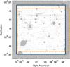 |
Fig. 1 VLA-COSMOS 3 GHz Large Project mosaic with grayed-out regions masked in the COSMOS2015 catalog because of the presence of saturated or bright sources in the optical to NIR bands. Also indicated are the areas covered by Subaru Suprime Cam (blue full line, corresponding to the outer edge of the unmasked area), and UltraVISTA (Ultra Deep Survey with the VISTA telescope; orange dash-dotted line; see Laigle et al. 2016 and references therein). The masked regions reduce the effective area to 1.77 deg2 with 8696 (80%) out of 10 830 radio sources outside the masked areas. |
Given the onset of upcoming revolutionary radio facilities, such as the Square Kilometre Array (SKA)2 (Norris et al. 2013; Prandoni & Seymour 2015) and the Next Generation Very Large Array (ngVLA)3 (Hughes et al. 2015), scheduled to be operational at the same time as the Large Synoptic Survey Telescope (LSST)4 and Euclid5, it becomes even more important i) to study the composition of the radio source population as a function of radio flux density, probing the to-date faintest achievable flux limits over significant areas and accounting for the possibility of a composite nature of galaxies containing both AGN and star formation activity; and ii) to make predictions that are applicable to future radio surveys, facilitating the identification of the various galaxy populations within these surveys. The COSMOS project (Scoville et al. 2007) is optimal for such research as it is currently one of the most advanced panchromatic surveys covering a 2 square degree area and sampling galaxies and AGN out to high (z ≲ 6) redshift. This project incorporates one of the deepest radio data sets ever obtained with the VLA at 3 GHz detecting 10 830 sources down to ≈ 11.5 μJy (≈ 5σ at an angular resolution of 0.75″; Smolčić et al. 2017a). Here we combine these radio data with the COSMOS X-ray to FIR multiwavelength data sets to search for counterparts of the radio sources and analyze the composition of the faint microJansky radio population, extrapolating this down to the flux limits that will be achieved with the SKA in Phase 1 (SKA1; Prandoni & Seymour 2015).
In Sect. 2 we describe the data sets used in the analysis. Section 3 summarizes the method of association of multiwavelength, optical-MIR counterparts to our radio sources; the details of this method are given in Appendix A. In Sect. 4 we introduce the X-ray counterparts to our radio sources. In Sect. 5 we analyze the redshifts of the counterparts. In Sect. 6 we present a multiwavelength assessment of the galaxy populations present within our radio source sample. In Sect. 7 we present the counterpart and source population catalog released. The composition of the microJansky radio source counts in the context of different galaxy populations and emitting mechanisms in the radio are discussed in Sect. 8. We summarize in Sect. 9. Throughout this paper, magnitudes are given in the AB system, coordinates in the J2000 epoch, and we use the following cosmological parameters: ΩM = 0.3, ΩΛ = 0.7 and H0 = 70 km s-1 Mpc-1. We define the radio spectral index, α, via Sν ∝ να, where Sν is the flux density at frequency ν. A Chabrier (2003) initial mass function (IMF) is used.
2. Data
In this section we describe the multiwavelength data used in the analysis.
2.1. Radio data
The VLA-COSMOS 3 GHz Large Project entails 384 h of observations with the VLA in S band centered at 3 GHz with 2048 MHz bandwidth over a total area of 2.6 square degrees (see Smolčić et al. 2017a for details). The VLA S band was chosen for the observations as the combination of a large effective bandwidth (~ 2 GHz) and fairly large field of view of a half-power beam width 15′ 6 allow for a time-efficient coverage of a field such as COSMOS (~ 2 square degrees) to a high sensitivity, even though the sources detected are typically fainter at this observing frequency compared to the commonly used 1.4 GHz observing frequency (L band)7. The observing layout was such that a uniform rms, with a median rms ~ 2.3 μJy/beam (at a resolution of 0.75″), was reached over the inner 2 square degrees coincident with the (Subaru Suprime Cam) COSMOS field (see Fig. 1). Over the full 2.6 square degrees the survey yielded a total of 10 830 cataloged sources. Of these, 67 were found to be multicomponent sources, i.e., objects that are composed of two or more detected radio components that are completely separated from each other, but belong to the same source (see Smolčić et al. 2017a; Vardoulaki et al., in prep.). The combination of the multiple components into one reported source was performed by visual inspection using the auxiliary multiwavelength data available in the COSMOS field (see Smolčić et al. 2017a). These sources are mainly radio galaxies with resolved core/jet/lobe structures (see Fig. 7 in Smolčić et al. 2017a), but can also be star-forming galaxies where the radio emission follows the disk morphology. The remaining 10 763 detected sources are referred to as single-component sources.
Prior to the VLA-COSMOS 3 GHz Large Project, the field was observed with the VLA at 1.4 GHz frequency within the VLA-COSMOS 1.4 GHz Pilot, Large, and Deep Projects (Schinnerer et al. 2004, 2007, 2010). Within the 1.4 GHz Large Project a uniform rms of 10–15 μJy/beam was reached over a resolution element of 1.5″ across the 2 square degree field. The Deep Project added further observations toward the inner square degree, yielding an rms of 12 μJy/beam over a resolution elements of 2.5″. A joint catalog was generated combining the sources detected at ≥5σ at 1.5″ and/or 2.5″ resolution in the Large and/or Deep Projects, and lists a total of 2864 sources (Schinnerer et al. 2010). Matching the 3 GHz catalog with the joint 1.4 GHz catalog using a radius of 1.3″, which corresponds to approximately half the synthesized beam size at 1.4 GHz, yields 2530 matches (see Smolčić et al. 2017a). Hence, for 2530 out of 10 830 sources in the 3 GHz catalog a spectral index can be calculated based on the two frequencies. For the remainder of the sources a spectral index of –0.7 is assumed that is consistent with the average value derived for the full 3 GHz population also taking into account limits of the spectral indices for sources detected at 3 GHz, but not detected at 1.4 GHz (for more details see Sect. 4.2. and Fig. 14 in Smolčić et al. 2017a). It is widespread in the literature to assume a single spectral index for the radio spectral energy distribution (SED; usually taken to be α = −0.7 or α = −0.8). The usually observed spread in spectral indices is σ ≈ 0.35 (e.g., Smolčić et al. 2017a) and the uncertainty of the spectral index can induce significant errors in the derived radio luminosity for a single object. However, on a statistical basis the symmetry of the spread is expected to cancel out the variations yielding a valid average luminosity for the given population (see also Novak et al. 2017; Delhaize et al. 2017; Smolčić et al. 2017b, for more specific discussions on this).
2.2. Near-ultraviolet – mid-infrared data and photometric redshifts
To complement our data set with optical, near-infared (NIR), and MIR wavelengths we use i) the latest photometry and photometric redshift catalogs (COSMOS2015 hereafter; Laigle et al. 2016); ii) the i band selected catalog (version 1.8, Capak et al. 2007); and iii) the Spitzer – COSMOS (S-COSMOS) InfraRed Array Camera8 3.6 μm selected catalog (IRAC hereafter; Sanders et al. 2007).
The COSMOS2015 catalog lists optical and NIR photometry in over 30 bands for 1 182 108 sources identified either in the z++YJHKS9 stacked detection image (within the area encompassed by the Ultra Deep Survey with the VISTA telescope, UltraVISTA, where YJHKS are taken from UltraVISTA DR210), or the z++ band, outside the UltraVISTA footprint (see Fig. 1). The total area covered by the catalog used is ~ 2.3 square degrees, which reduces to an effective area of 1.77 square degrees if masked regions are excluded. The cataloged fluxes were extracted as described in detail by Laigle et al. (2016), using SExtractor on the positions of the sources detected in the stacked images separately for 2″ and 3″ diameter apertures; corrections to total magnitudes are given for each source as well as corrections for galactic dust extinction from Schlegel et al. (1998). The point spread functions (PSFs) were homogenized in the optical/NIR maps to a resolution of  prior to extraction of the COSMOS2015 catalog. The 3σ limits for 2″ (3″) diameter apertures are 25.9 (26.4) for z++, and 24.8 (25.3), 24.7 (25.2), 24.3 (24.9), 24.0 (24.5) for the Y, J, H, KS Deep bands, respectively (see Table 1 and Figs. 1–3 in Laigle et al. 2016 for more details). The above-mentioned procedure was also used to extract the four IRAC band photometry, where particular care was taken to properly deblend the IRAC photometry using IRACLEAN (see Laigle et al. 2016 for details). The IRAC channel 1 and 2 data were drawn from the SPLASH survey (PI: P. Capak), while channels 3 and 4 were taken from the S-COSMOS survey (see also below). The 3σ depths for 3″ apertures in IRAC channel 1–4 are 25.5, 25.5, 23.0, and 22.9 (mAB), respectively. In addition, this data set also contains 24μm photometry from Le Floc’h et al. (2009) from the Multi-Band Imaging Photometer for Spitzer (MIPS) down to a magnitude limit of 19.45. Laigle et al. (2016) have computed photometric redshifts for the sources listed in the COSMOS2015 catalog using LePhare (see also Ilbert et al. 2009, 2013). They report a photometric redshift accuracy11 within the UltraVISTA-COSMOS area of σΔz/ (1 + zs) ~ 0.01 for 22 <i+< 23, and σΔz/ (1 + zs)< 0.034 for 24 <i+< 25 based on comparison with a spectroscopic redshift sample in the COSMOS field (cf. Table 4 in Laigle et al. 2016).
We also use the i band selected COSMOS photometric catalog version 1.8 (initially described in Capak et al. 2007). This catalog contains 2 017 800 i band selected sources, and 15 photometric bands ranging from 0.3 μm to 2.4 μm, measured in 3″ diameter apertures. The total area covered is ~ 3.1 square degrees. The 5σ depth in a 3″ aperture is  . The catalog has been cross-matched with MIPS 24μm data from Le Floc’h et al. (2009) and also contains photometric redshifts derived by Ilbert et al. (2009) using LePhare with an accuracy similar to that reached for the COSMOS2015 sources. The PSF-homogenized images have a resolution of θ ~ 0.̋8, as in the COSMOS2015 catalog. In comparison to the i band selected COSMOS catalog (Capak et al. 2007) within the 1.5 square degree area of the COSMOS field covered by UltraVISTA, Laigle et al. (2016) show that 96.5% (83.9%) of sources brighter than Subaru i+ = 25.5 (26.1) are also detected in the COSMOS2015 catalog. Thus, given that some of the i band selected sources are not recovered in the COSMOS2015 catalog, we also make use of the i band selected COSMOS catalog.
Additionally, we use the Spitzer IRAC catalog (Sanders et al. 2007) of 345 512 sources detected (≳1 μJy) at 3.6 μm, over an area of ~ 2.8 square degrees. This catalog includes photometry in the four IRAC channels at 3.6, 4.5, 5.6, and 8.0 μm, for sources detected in the 3.6 μm image. Their respective 3σ depths are 24.6, 23.8, 21.8, and 21.6. For each channel, fluxes extracted within four apertures are given. We use the 1.̋9 aperture photometry given in the catalog. The 3.6 μm image resolution is θ =1.̋66.
The combined use of the three catalogs increases the likelihood of finding counterparts to radio sources, especially those (either very blue or very red) counterparts whose SED makes them undetectable in the stacked z++YJHKS map of COSMOS2015 but that are detected in the i band or IRAC. Furthermore, highly obscured and/or high redshift sources might only be detectable in the 3.6 μm IRAC band.
2.3. Far-infrared and (sub-)millimetre photometry
To derive accurate estimates of the SFR of each radio source, we use far-infrared photometry from the Herschel Space Observatory, which encompasses the full 2 square degrees of the COSMOS field. Herschel imaging is taken from the Photoconductor Array Camera and Spectrometer (PACS; 100 and 160μm; Poglitsch et al. 2010) and Spectral and Photometric Imaging Receiver (SPIRE; 250, 350, and 500μm; Griffin et al. 2010), which are part of the PACS Evolutionary Probe (PEP; Lutz et al. 2011) and the Herschel Multi-tiered Extragalactic Survey (HerMES; Oliver et al. 2012) projects. The COSMOS2015 catalog (Laigle et al. 2016) reports the deblended Herschel fluxes extracted using 24μm positions as priors (from Le Floc’h et al. 2009) and unambiguously associated with the corresponding optical/NIR counterpart via 24μm IDs reported in both catalogs. A similar association technique is applied to assign Herschel counterparts to i band selected sources (Capak et al. 2007).
In addition to far-infrared data, we also retrieve the available (sub)-millimetre photometry from at least one of the observational campaigns conducted over the COSMOS field: JCMT/SCUBA-2 at 450 and 850μm (Casey et al. 2013), LABOCA at 870μm (F. Navarrete et al., priv. comm.), Bolocam (PI: J. Aguirre), JCMT/AzTEC (Scott et al. 2008) and ASTE/AzTEC (Aretxaga et al. 2011) at 1.1 mm, MAMBO at 1.2 mm (Bertoldi et al. 2007), and interferometric observations at 1.3 mm with PdBI (Smolčić et al. 2012; Miettinen et al. 2015) and ALMA (PI: M. Aravena; Aravena et al., in prep.).
2.4. X-ray data
We use the most recent COSMOS X-ray catalog of point sources (Marchesi et al. 2016), drawn from the Chandra COSMOS-Legacy survey (Civano et al. 2016). The Chandra COSMOS-Legacy survey combines the Chandra COSMOS (Elvis et al. 2009) data with the new Chandra ACIS-I data (2.8 Ms observing time) resulting in a total exposure time of 4.6 Ms over 2.15 deg2 area, reaching (at best) a limiting depth of 2.2 × 10⁻¹⁶ erg s-1 cm-2 at [0.5–2] keV, 1.5 × 10⁻¹⁵ erg s-1 cm-2 at [2–10] keV, and 8.9 × 10⁻¹⁶ erg s-1 cm-2 at [0.5–10] keV (Civano et al. 2016). The X-ray observations cover the central 1.5 square degrees of the COSMOS field with an average effective exposure time of 160 ks, while in the outer regions it reduces down to 80 ks. The catalog contains 4016 X-ray point sources in the Chandra COSMOS-Legacy survey, out of which 3877 have optical–MIR counterparts, matched using the likelihood ratio technique (Marchesi et al. 2016). The counterparts were searched for in three different bands. The i band (760 nm) was taken from Subaru where the data was unsaturated (iAB> 20; Capak et al. 2007) and from CFHT and SDSS otherwise. Matching was also carried out with the Spitzer IRAC catalog (Sanders et al. 2007) and the SPLASH IRAC magnitudes from Laigle et al. (2016), in which the photometry was extracted at positions with a detection in the z++YHJKS stacked image, as described in more detail in the previous section. The catalog lists X-ray fluxes and intrinsic, i.e., unobscured, X-ray luminosities in the full [0.5–10] keV, soft [0.5–2] keV, and hard [2–10] keV X-ray bands. Later on, X-ray fluxes and luminosities are given up to 8 keV, by assuming a simple power-law spectrum with photon index Γ = 1.4 (Marchesi et al. 2016). Also, spectroscopic or photometric redshifts of the X-ray sources are available in the catalog (see Civano et al. 2016).
2.5. Spectroscopic redshifts
We use the most up-to-date spectroscopic redshift catalog available to the COSMOS team (see Salvato et al., in prep.). It contains 97 102 sources with spectroscopic redshifts. The catalog has been compiled from a number of spectroscopic surveys of the COSMOS field, including SDSS (DR12), zCOSMOS (Lilly et al. 2007, 2009), VIMOS Ultra Deep Survey (VUDS; Le Fèvre et al. 2015), MOSDEF (Kriek et al. 2015), and DEIMOS12.
3. Optical-MIR counterparts
In this section we describe the cross-correlation of our radio sources with optical (i band-selected), NIR (z++-, or z++YJHKS-stack-selected, COSMOS2015), and MIR (3.6 μm-selected, IRAC) sources. We here report the numbers of optical-MIR counterparts associated with our radio sources within the same unmasked area of 1.77 deg2 (see Fig. 1), while in Appendix B we present the full counterpart catalog that also includes sources outside the 1.77 deg2 area. We separately associate the multicomponent and single-component radio sources with their optical-MIR counterparts, as detailed in Sects. 3.1, and 3.2, respectively. We present an assessment of the optical-MIR counterparts of our radio sources in Sect. 3.3.
3.1. Counterparts of multicomponent radio sources
Out of the 67 multicomponent radio sources identified in our 3 GHz radio catalog, 48 lie within the optical-MIR unmasked area of 1.77 deg2. By visual inspection we find a match for all 48 sources in the COSMOS2015 catalog, accounting for the full sample of multicomponent radio sources (see Table 1).
3.2. Counterparts of single-component radio sources
The optical-MIR counterpart assignment to our single-component 3 GHz radio sources is described in detail in Appendix A and here we only present a brief overview. We base the counterpart association on nearest neighbor matching, accounting for a false match probability (pfalse) for each match. The counterpart association proceeded as follows.
First, prior to the positional matching of our 3 GHz sources separately to the sources from the COSMOS2015 (Laigle et al. 2016), i band (Capak et al. 2007), and IRAC (Sanders et al. 2007) catalogs the astrometry in each multiwavelength catalog was corrected for observed small systematic offsets relative to the radio positions (see Appendix A.1). Second, a positional matching of the 3 GHz radio sources was performed with the sources in the unmasked areas of each of the COSMOS2015, i band, and IRAC catalogs out to a search radius of  (COSMOS2015/i band), or
  (IRAC). Third, a false match probability was assigned to every counterpart match based on Monte Carlo simulations. For the simulations we matched sources from mock catalogs that realistically reflect the magnitude and separation distributions expected for the counterparts of our radio sources (see Appendix A.2 for details). These steps led to three counterpart candidate catalogs, each, respectively, containing the 3 GHz sources matched to sources from the 1) COSMOS2015 (see Appendix A.3); 2) i band (see Appendix A.4); and 3) IRAC catalogs (see Appendix A.5) with a false match probability computed for each match.
In the fourth, final step, only one final counterpart of a given 3 GHz source is selected from the three catalogs following a hierarchical line of reasoning, setting first, second, and third priority to the COSMOS2015, i band, and IRAC matches, respectively. The hierarchical choice was based on a combination of critetia, such as best resolution, and therefore more precise positions, and the availability of accurate photometric redshifts that were computed via the to-date best available, i.e., deepest photometry.
In this last step, we associate with the 3 GHz single-component sources counterparts from the COSMOS2015 catalog if they are present within 0.̋8 and have pfalse ≤ 20%, or if they have pfalse> 20%, but coincide with a reliable (pfalse ≤ 20%) counterpart candidate from either of the other two catalogs (in total, 7681 COSMOS2015 counterparts, 57 of which belong to the second category). We associate i band counterparts if they are within 0.̋8 and have pfalse ≤ 20% and do not coincide with a COSMOS2015 counterpart candidate, or if they have pfalse> 20%, but coincide with a reliable (pfalse ≤ 20%) counterpart candidate from the IRAC catalog (in total, 97 i band counterparts, 39 of which belong to the second category). Otherwise, we associate IRAC counterparts (209 IRAC counterparts, in total). Additionally, we do not allow the same multiwavelength counterpart being associated with different 3 GHz sources following the same reasoning approach.
Summary of the cross-correlation of the VLA-COSMOS 3 GHz Large Project sources with sources in the multiwavelength catalogs.
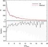 |
Fig. 2 Top: signal-to-noise ratio distribution of all (black line) and matched (red dashed line) VLA 3 GHz single-component sources. Bottom: fraction of matched VLA 3 GHz single-component sources as a function of signal-to-noise ratio. Poisson errors are also shown. |
3.3. Assessment of optical-MIR counterparts
The final counterparts assigned to both our multi- and single-component 3 GHz radio sources are summarized in Table 1. Overall, 772913, 9714, and 20915 3 GHz sources are associated with COSMOS2015, i band, and IRAC counterparts, respectively. In total, we find 8035 counterparts for our radio sources. Summing the computed false match probabilities we estimate a total fraction of spurious matches of ~ 2%. Since our identification procedure is based on ground-based catalogs, it is likely that this “formal” fraction should be considered a lower limit because of the limited spatial resolution of these data used in these catalogs. The number of radio sources within the unmasked 1.77 deg2 area is 8696, which yields an overall counterpart fraction of 92.4% (i.e., 8035/8696).
In Fig. 2 we show the 3 GHz S/N distribution for all the 8696 and the matched 8035 radio sources. The fraction of identifications is greater than ~90% for radio sources with a signal-to-noise ratio ≳6, below which decreases to ~80% at a signal-to-noise ratio of 5. Such a trend is not surprising as the estimated fraction of spurious radio detections increases at the lowest signal-to-noise ratios; the fraction of false detections is 24% for signal-to-noise ratios between 5.0 and 5.1, which decreases to less than 3% beyond signal-to-noise ratios of 5.5 (see Fig. 17 in Smolčić et al. 2017a).
4. X-ray counterparts
We used the X-ray point-source catalog from Marchesi et al. (2016) (described in detail in Sect. 2) to match the X-ray and radio sources. We matched the counterparts of the X-ray sources to the counterparts of the radio sources. Given that the same (COSMOS2015, i band, and IRAC) catalogs have been used to assign counterparts to X-ray and radio-detected sources via either a likelihood ratio technique (Marchesi et al. 2016) or a nearest neighbor match with false match probability assigned as carried out here, the clearest way to match the X-ray and radio sources is to take their assigned counterparts (see, e.g., Smolčić et al. 2008).
Marchesi et al. (2016) list the IDs of the COSMOS2015 and i band counterparts of X-ray sources. Thus, after associating our radio sources with counterparts from the COSMOS2015 and the i band selected catalog, we match their respective IDs to those given in the X-ray catalog. The radio sources with IRAC counterparts were cross-matched to the X-ray catalog via a nearest neighbor matching between IRAC positions listed in both catalogs, but using a search radius of 0.̋1 to account for machine rounding error. In total, we find 927 X-ray counterparts to our radio sources with COSMOS2015 (906), i band (5) or IRAC (16) counterparts. Among the 927 X-ray counterparts, 592 (64%) of the redshifts reported by Marchesi et al. (2016) are spectroscopic, 325 (35%) are photometric, and 10 (1%) do not have a redshift listed.
For X-ray sources with redshift values given in the catalog from Marchesi et al. (2016), we use the intrinsic (i.e., unobscured) X-ray luminosities already provided in the catalog. In case an X-ray source does not have a spectroscopic or photometric redshift available in the Marchesi et al. (2016) catalog (about 10 in total entering our sample), we assign it a redshift by taking the most reliable spectroscopic or photometric measurement available in the literature, as described in Sect. 5. The corresponding X-ray luminosity (Lx) is calculated by following the same approach detailed in Marchesi et al. (2016), which uses the hardness ratio as a proxy for nuclear obscuration (see also Xue et al. 2010). The unobscured Lx estimates were then scaled from [0.5–10] keV to [0.5–8] keV by assuming a power-law spectrum with intrinsic slope Γ = 1.8 (e.g., Tozzi et al. 2006).
5. Redshifts of VLA 3 GHz source counterparts
We gathered redshift measurements of the radio source counterparts by taking the most reliable redshift available in the literature, either spectroscopic or photometric, as described in Delvecchio et al. (2017) for only the subset of COSMOS2015 counterparts analyzed here (see their Sect. 2.3), and extended these to the full list of COSMOS2015, i band, and IRAC radio source counterparts.
For the COSMOS2015 and i band counterparts that were not detected in X-ray, the photometric redshifts were taken from their respective catalogs. These were derived using the LePhare SED-fitting code (Arnouts et al. 1999; Ilbert et al. 2006), as described in Ilbert et al. (2009, 2013). Photometric redshift estimates for IRAC counterparts were found by cross-matching to COSMOS2015 or i band sources within the respective masked regions. For X-ray detected sources, we used a different set of photometric redshifts from Salvato et al. (in prep.), which were obtained via SED fitting that included AGN variability and AGN templates (Salvato et al. 2009, 2011); thus these estimates are more suitable for AGN-dominated sources.
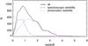 |
Fig. 3 Redshift distribution of the matched (COSMOS2015 and i band) counterparts with redshifts. The black solid line shows the distribution of the best available spectroscopic or photometric redshifts, the red dotted line that of the photometric redshift subsample, while the blue dot-dashed line that of the spectroscopic redshift subsample. |
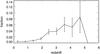 |
Fig. 4 Fraction of i band only counterparts in the total (COSMOS2015 and i band counterparts combined) as a function of redshift. Poisson errors are also shown. |
For each counterpart reported in the spectroscopic sample compiled by Salvato et al. (in prep.), we only replaced the photometric redshift with the spectroscopic redshift if the spectroscopic measurement was considered “secure” or “very secure”16. Additional 28 spectroscopic redshifts were taken from the VIMOS Ultra Deep Survey (VUDS; Le Fèvre et al. 2015; Tasca et al. 2017). For X-ray detections, in addition to the above criteria, we adopted the best available redshift reported in Marchesi et al. (2016).
In total, we retrieved a redshift value for 7778 out of 8035 sources (~98% of our sample); 2740 (~34%) are spectroscopic and 5123 (~64%) are photometric. The 124 sources (corresponding to ~2% of the sample) with no redshift measurement were associated with an IRAC-only counterpart. The mean redshift for the remaining IRAC sources is similar to the mean values of the counterparts in the COSMOS2015 and i band catalogs (z ~ 1.3). The counterpart redshift distribution is shown in Fig. 3. We also verified the accuracy of the photometric redshifts in our sample based on the comparison with the available spectroscopic measurements. We found a dispersion of the | Δz/ (1 + z) | distribution of σ| Δz/ (1 + z) | = 0.01, peaking at 0.002 (see also Laigle et al. 2016).
Having assigned redshifts to the counterparts of our 3 GHz sources, we now assess the potential incompleteness of the COSMOS2015 catalog, cross-correlated with the 3 GHz radio source catalog (cf. Fig. 8 in Laigle et al. 2016). In Fig. 4 we show the fractional contribution of the i band counterparts to the total COSMOS2015 and i band counterpart sample. We find that the incompleteness (i.e., the largest fraction of i band-only counterparts) rises with increasing redshift from ≲1% at z< 2 to ~ 8% close to z = 5.
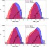 |
Fig. 5 Magnitude distributions for the 3 GHz radio source counterparts with available IRAC magnitudes, separated into three subsamples as indicated in the right panels. |
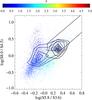 |
Fig. 6 MIR color–color diagram for 6793 radio sources with available spectroscopic or photometric redshifts and IRAC magnitudes (symbols), color coded according to their redshift value, as indicated in the color bar at the top. The blue lines indicate the 2D density contours for the sample with IRAC counterparts (205 sources), while the black lines represent the 2D density contours for IRAC counterparts without a redshift measurement (122 objects). The black wedge indicates the Donley et al. (2012) area for the selection of MIR-AGN in this color–color plane. |
In Fig. 5 we show the distributions for each IRAC band separately for a subset of radio sources with available IRAC fluxes in all channels (6915 sources) and for the various subsets of sources with spectroscopic redshift (2674 sources), photometric redshift (4119 sources), and without redshift (122 sources). As expected, for all IRAC bands these subsets lie at different magnitude ranges, for which the spectroscopic redshifts are more common for brighter sources, followed by those with photometric redshifts, and eventually by those without redshifts at the faint tail of the magnitude distribution.
In Fig. 6 we show the IRAC color–color distribution for the radio sources with available redshift and fluxes in all IRAC bands (6793 sources). While the IRAC color distribution and average redshift are similar between the full sample and the subsample with IRAC-only counterparts, the 122 sources with no redshift show redder colors and a distribution consistent with being at z> 1. The bulk of these sources falls within the wedge defined by Donley et al. (2012) for the selection of MIR-AGN in this color–color plane, suggesting a possible AGN nature of a significant fraction of them.
6. Galaxy populations
In this section we characterize the galaxy populations present in our 3 GHz survey. Our aim is to assess the multiwavelength properties of our 3 GHz sources, such that various characteristics can be combined to select AGN/star-forming galaxy samples depending on the scientific application, for example, either i) conservative/cleaned AGN or star-forming galaxy samples or ii) parent populations of radio AGN or star-forming galaxies with clean selection functions beyond the radio regime (but contaminated to a degree, as quantified below). For example, the latter (i.e., a selection not relying on radio flux/luminosity) is preferable for the purpose of, for example, stacking in the radio map (e.g., Karim et al. 2011) or statistically assessing radio-AGN duty cycles (e.g., Smolčić 2009). Furthermore, the multiwavelength properties of our sources identified via various (nonradio and radio-based selection criteria) shed light on the composite AGN plus star-forming nature of our sources over a broad wavelength range and in particular in the radio regime. For sources with available redshifts (i.e., COSMOS2015 or i band counterparts) we first identify AGN with a combination of X-ray, MIR, and SED fit criteria. For the remainder of the sample we then identify star-forming galaxies and AGN based on the rest-frame optical colors of their host galaxies (Sect. 6.1). We then analyze the properties of the galaxy samples in terms of excess of radio emission relative to the SFRs in their host galaxies, which can be attributed to AGN activity in the radio (Sect. 6.2), and radiative bolometric luminosities of the identified AGN (Sect. 6.3). We categorize and summarize the samples in Sect. 6.4. For the following analysis we use the (7826) 3 GHz sources with COSMOS2015 (7729) or i band (97) counterparts present in the unmasked areas of the given catalogs (see Fig. 1 and Table 1), i.e., within a well-defined, unbiased effective area of 1.77 square degrees. We also stress that the multiwavelength assessment as presented here is statistical in nature. While the classification is not be correct for every single radio source, it is statistically correct for the population as a whole.
6.1. X-ray to far-infrared signatures of AGN and star formation activity
6.1.1. X-ray-, MIR, and SED-selected AGN
Physical processes present in AGN imprint their signature onto the emitted radiation. Powerful X-ray emission from radio sources has been found to originate in a radiatively efficient mode of accretion onto the central black hole (e.g., Evans et al. 2006). These AGN may also be identified via emission from a warm dusty torus around the central black hole that is detectable in the MIR (Donley et al. 2012). Thus, we identify X-ray AGN as those with a [0.5–8] keV X-ray luminosity higher than 1042 erg s-1; MIR AGN are identified with IRAC color–color criteria; and those that show AGN signatures in the multiwavelength SED are identified using SED-fitting decomposition to disentangle the AGN emission from the host-galaxy light. Below we summarize the selection, and refer to Delvecchio et al. (2017) for a detailed analysis of the physical properties of such selected AGN across cosmic time.
To select X-ray AGN, we have chosen a limit in intrinsic [0.5–8] keV (i.e., unobscured) X-ray luminosity of LX = 1042 erg s-1 (e.g., Szokoly et al. 2004). We verified that the X-ray emission expected from the IR-based SFR (obtained from SED-fitting; see below) is generally negligible (i.e., a few %) compared to the observed X-ray emission, by assuming a canonical LX–SFR conversion by Symeonidis et al. (2014). This is always true for X-ray sources with LX ≥ 1042 erg s-1. For this reason, we consider all sources in our sample with LX above that limit to be AGN. From our sample of 7826 radio sources with COSMOS2015 or i band counterparts, 859 (~11%) are selected as X-ray AGN. While all the sources with an X-ray luminosity higher than the adopted threshold are likely to be AGN, we cannot exclude that AGN are also present in the sample of X-ray sources with an X-ray luminosity lower than the threshold. Indeed, out of the X-ray sources with LX< 1042 erg s-1, ~ 33% have been already classified as AGN using other criteria (described below). Given the typical X-ray flux in the COSMOS field, this X-ray selection of AGN is progressively missing faint AGN at high redshift, where the X-ray limiting luminosity is higher than 1042 erg s-1 (see, for example, Fig. 8 in Marchesi et al. 2016).
To complement the X-ray selection criterion, we adopted the MIR selection method of Donley et al. (2012). It allows for a reliable selection of sources that contains a warm dusty torus that is consistent with those in standard, thin-disk AGN (Shakura & Sunyaev 1973), and although reliable, it is not complete. This classification relies on the four IRAC bands at 3.6, 4.5, 5.8, and 8 μm. Dusty tori of AGN are found within a wedge in that diagram, but also imprint a monotonic rise of flux through the four MIR bands. Sources found displaying these characteristics were recognized as MIR AGN. Although 229 (~27%) of the sources classified as X-ray AGN also satisfy the MIR AGN criteria, 237 sources in our total sample of COSMOS2015 and i band counterparts fit the MIR AGN criterion, while not satisfying the X-ray criterion. Thus, the MIR AGN selection can be considered complementary to the X-ray AGN selection method (see also Delvecchio et al. 2017). In total, we find 466 MIR AGN in our sample of 7826 3 GHz sources matched with COSMOS2015 or i band counterparts.
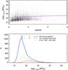 |
Fig. 7 Top panel: ratio of rest-frame 1.4 GHz radio luminosity and infrared SFR, log (L1.4 GHz/SFRIR), as a function of redshift. The curve indicates the redshift-dependent threshold used to identify radio excess sources (see text for details). Bottom: distribution of log (L1.4 GHz/SFRIR) for various (nonoverlapping) galaxy populations as indicated in the panel. The vertical lines indicate the (bi-weighted) means of the distributions. |
Lastly, we fit the optical to millimetre SED17 of each radio source to identify possible evidence of AGN activity on the basis of a panchromatic SED-fitting analysis (originally developed by da Cunha et al. 2008, and expanded by Berta et al. 2013). We adopt the fitting results already performed for the COSMOS2015 counterparts by Delvecchio et al. (2017) and use the same approach to fit the SEDs of the i band counterparts. The three-component SED fitting code SED3FIT by Berta et al. (2013)18 is used to disentangle the possible AGN contribution from the host-galaxy light. This approach combines the emission from stars, dust heated by star formation and a possible AGN/torus component (Feltre et al. 2012, see also Fritz et al. 2006). The dust-absorbed UV-optical stellar light is linked to the reprocessed far-IR dust emission by energy balance. To quantify the relative incidence of a possible AGN component, we followed the approach described in Delvecchio et al. (2014), by fitting each source SED with both the magphys code and the three-component SED-fitting code. The fit obtained with the AGN is preferred if the reduced χ2 value of the best fit is significantly (at ≥99% confidence level, on the basis of a Fisher test) smaller than that obtained from the fit without the AGN. We find 1178 COSMOS2015 or i band counterparts fulfilling this criterion (out of these 669 are also identified as X-ray or MIR AGN; see Fig. 2 in Delvecchio et al. 2017), which hereafter are referred to as SED-AGN. In summary, we identify a total of 1623 AGN by combining X-ray-, MIR-, and SED-selected AGN.
6.1.2. Optically selected AGN and star-forming galaxies
Having exploited the X-ray, MIR-, and SED-based AGN selection criteria (see Sect. 6.1.1), we next use a UV/optical color-based separation method developed by Ilbert et al. (2010) to derive the composition of the remaining galaxy population. This method separates sources based on the rest-frame near ultraviolet (NUV) minus r+ band colors corrected for internal dust extinction (MNUV−Mr). In the work of Ilbert et al. (2010), sources are considered quiescent if MNUV−Mr> 3.5, of intermediate (star formation) activity if 1.2 <MNUV−Mr< 3.5, and of high (star formation) activity if MNUV−Mr+< 1.2. Ilbert et al. (2010) verified these color selection criteria via a comparison with other color selections, morphology, and specific SFRs of their galaxies (see Figs. 4–6, and 9 in Ilbert et al. 2010). Following this selection here we define the “intermediate activity” and “high activity” galaxies as star-forming galaxies (SFGs hereafter), and we also include galaxies with red (MNUV−Mr+> 3.5) colors in this class, when detected in the Herschel bands. The latter have properties consistent with star-forming, rather than quiescent AGN galaxies (e.g., Delhaize et al. 2017). The remaining, red galaxies, which are not detected in the Herschel bands, are then quiescent galaxies, consistent with typical properties of radio AGN host galaxies, as verified in a number of previous studies (e.g., Best et al. 2006; Donoso et al. 2006; Sadler et al. 2014; Smolčić 2009). Thus, they can be taken as radio-detected AGN hosted by quiescent red galaxies (see also below). In total, we identify 5410 SFGs, and 793 red quiescent AGN hosts.
6.2. Radio excess as AGN signature in the radio band
In the previous sections we identified AGN and SFGs in our 3 GHz radio source sample, based on their multiwavelength (X-ray to FIR) properties. We here investigate the excess radio emission relative to the SFRs in their host galaxies. This yields an insight into the AGN origin of the radio emission in these galaxies, which may not necessarily be in one-to-one correspondence with, for example, AGN signatures in the X-ray or MIR bands, hence shedding light on the composite nature of the sources.
In Fig. 7 we show the distribution of log (L1.4 GHz/SFRIR), i.e., the logarithm of the ratio of the 1.4 GHz rest-frame radio luminosity and SFR derived from the total IR emission in the host galaxies as computed via the three-component SED-fitting procedure as described above and by Delvecchio et al. (2017). The SFRs were obtained from SED fitting using the total (8–1000μm rest-frame) infrared luminosity obtained from the best-fit galaxy template for sources both with and without Herschel detection, as described in Delvecchio et al. (2017). This luminosity represents the fraction of the total infrared luminosity arising from star formation for X-ray-, MIR-, and SED-selected AGN, or the total IR luminosity otherwise, and was converted to SFR via the Kennicutt (1998) conversion factor and scaled to a Chabrier (2003) IMF. As radio luminosity is an efficient star formation tracer (i.e., log SFR = log L1.4 GHz + const.; e.g., Condon 1992), an excess in log (L1.4 GHz/SFRIR) can be taken as arising from non-SFR, thus AGN-related processes in the radio band. Given a positive trend of log (L1.4 GHz/SFRIR) with redshift (see also Delhaize et al. 2017), following Delvecchio et al. (2017) we use a redshift-dependent threshold of the form log (L1.4 GHz/SFRIR) = 21.984(1 + z)0.013 to better quantify the excess in radio emission relative to the star formation in the host galaxies in our sample (radio excess hereafter). For any given redshift range the dispersion (σlog (L1.4 GHz/SFRIR)) is derived by fitting a Gaussian to the distribution obtained by mirroring the distribution at the lower end over the distribution’s peak, thus eliminating the asymmetry of the distribution due to radio excess sources. The 3σ deviation from the peak of the Gaussian function at each redshift was chosen as the radio excess threshold.
The reason for a redshift-dependent threshold is purely observationally driven. A statistically more robust and detailed analysis (Delhaize et al. 2017), where both the radio and the FIR upper limits are fully taken into account, also finds that the median log (LIR/ 1.4 GHz) for our sample of star-forming galaxies shows a significant trend with redshift that is qualitatively consistent with what is shown in our Fig. 7 (see also, e.g., Magnelli et al. 2015; Calistro Rivera et al. 2017). Thus, the choice of a redshift-dependent threshold is fully consistent with the available observational data. Delhaize et al. discuss a number of possible reasons for this observed trend. These include, for example, the uncertainty in the radio SED shape (and therefore in the K correction), an AGN contribution in the SFG sample that possibly remains, and a systematic change with redshift, and/or with the level of SFR, of the average magnetic field of star-forming galaxies.
The above described redshift-dependent threshold in log (L1.4 GHz/SFRIR) yields a total of 1846 radio excess sources within the COSMOS2015/i band counterpart sample. Dissected per selection criterion (with possible overlap between various criteria), 277, 120, 337, 855, and 505 sources with radio excess have separately been identified as X-ray, MIR, SED AGN, star-forming, and red quiescent galaxies, respectively.
From Fig. 7 it is apparent that a large fraction of the radio AGN hosted by red quiescent galaxies show an excess of radio emission relative to the SFRs in their host galaxies, affirming their AGN nature at radio wavelengths. The SFG sample (selected based on green and blue optical rest-frame colors) occupies the region of the log (L1.4 GHz/SFRIR) distribution expected for star-forming galaxies, and consistent with no radio excess, with a tail extending toward higher radio excess About 16% (=1–4555/5410) of such identified SFGs exhibit a >3σ radio excess, which is taken as the contamination of this sample by radio-AGN identified via the >3σ radio excess in the log (L1.4 GHz/SFRIR) plane. This contamination of the SFG sample increases toward higher flux density levels, as shown in Fig. 8, where we also show the radio excess fractions as a function of radio flux for the red quiescent hosts and the combined X-ray, MIR, and SED AGN sample.
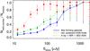 |
Fig. 8 Fraction of radio excess sources within the various galaxy samples (indicated in the panel) as a function of total 3 GHz radio flux. Poisson errors are also shown. |
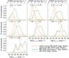 |
Fig. 9 Normalized distribution of bolometric (radiative) AGN luminosity (Lrad,AGN), as a function of redshift, for various populations, as indicated in the panels and legend, respectively. HLAGN refers to X-ray-, MIR-, and SED-selected AGN, while MLAGN refers to radio AGN hosted by red, quiescent galaxies or showing a >3σ radio excess in log (L1.4 GHz/SFRIR), but not selected as X-ray, MIR, or SED AGN (see text for details). Left-pointing arrows indicate upper limits in Lrad,AGN (see text for details). The upper x-axes show the supermassive black hole (SMBH) accretion rate that is estimated from Lrad,AGN assuming a standard radiative efficiency of 10%. |
 |
Fig. 10 Flowchart illustrating the separation of the 3 GHz sources matched to COSMOS2015 or i band counterparts (within unmasked areas of the field) into various AGN and galaxy populations (see Sect. 6 for details). |
The log (L1.4 GHz/SFRIR) distribution for the combined sample of X-ray, MIR, and SED AGN peaks close to that of star-forming galaxies and exhibits an extended tail toward higher values. As discussed in detail in Delvecchio et al. (2017) this suggests that a substantial amount of the radio emission in a large fraction of these AGN arises from star formation rather than AGN-related processes. However, there is also a large number of such sources with significant radio excess (~ 30% have a >3σ radio excess).
6.3. Radiative AGN luminosities
We here investigate the distribution of the radiative (bolometric) luminosities for the AGN identified here. We first combine the identified AGN into two categories: those that show AGN signatures i) at other than radio wavelengths, (i.e., X-ray-, MIR-, and SED-selected AGN; and ii) at radio wavelengths, i.e., those hosted by red quiescent galaxies, or showing a >3σ radio excess in log (L1.4 GHz/SFRIR), but not selected as X-ray, MIR, or SED AGN.
For each identified AGN the bolometric, radiative luminosity, or its upper limit was obtained from the best-fit SED template as described in detail by Delvecchio et al. (2017). Briefly, the AGN radiative luminosity is obtained from the best-fit AGN template. However, if the AGN template does not improve (at ≥99% significance, based on a Fisher test) the fit to the full SED, the corresponding AGN radiative luminosity is unconstrained from SED fitting. In this case, we report the 95th percentile of the corresponding probability distribution function, which is equivalent to an upper limit at 90% confidence level. The AGN radiative luminosities derived from the SED fitting have been compared with those independently calculated from X-rays, displaying no significant systematics and a 1σ dispersion of about 0.4 dex (see, e.g., Lanzuisi et al. 2015). In Fig. 9 we show the distribution of the AGN radiative luminosities for seven redshift bins out to z ~ 6. It is clear from this plot that the nonradio-based selection of X-ray, MIR, and SED AGN is, at every redshift, more efficient in selecting AGN with statistically higher radiative luminosities than AGN selection criteria mainly linked to radio wavelengths. Given that for the latter we only have upper limits to the radiative luminosity (left pointing arrows in Fig. 9), and that, thus, no unique separation threshold in radiative luminosity out to z ~ 6 can be inferred, we hereafter abbreviate the two identified categories19 as i) moderate-to-high radiative luminosity AGN (HLAGN hereafter, referring to X-ray-, MIR-, and SED-selected AGN, regardless of their radio excess in log (L1.4 GHz/SFRIR)); and ii) low-to-moderate radiative luminosity AGN (MLAGN hereafter, referring to the AGN identified via quiescent, red host galaxies, or those with a >3σ radio excess in log (L1.4 GHz/SFRIR), but not identified as X-ray, MIR, or SED AGN).
6.4. Sample summary
Using the multiwavelength criteria described above the identified AGN/star-forming galaxy samples can be categorized into three main classes of objects within our 3 GHz radio sample associated with COSMOS2015 or i band counterparts located inside the 1.77 square degree area unmasked in the COSMOS2015 catalog. The selection process and relative fractions of the three classes are illustrated in Fig. 10 and summarized below.
- 1.
Moderate-to-high radiative luminosity AGN (HLAGN) wereselected with a combination of X-ray(LX> 1042 erg/s), MIR color–color (Donley et al. 2012), and SED-fitting (Delvecchio et al. 2017) criteria. We identify a total of 1623 HLAGN in our 3 GHz sample consisting of 7826 radio sources with associated COSMOS2015 or i band counterparts and find that 486 (~ 30%) show a >3σ radio excess in log (L1.4 GHz/SFRIR), while the radio luminosity in the remaining ~70% is consistent (within ± 3σ) with the IR-based SFRs in their host galaxies.
- 2.
Star-forming galaxies (SFGs) were drawn from the sample remaining after exclusion of the HLAGN by selecting galaxies with the dust-extinction corrected rest-frame color i) MNUV−Mr+< 3.5 or ii) MNUV−Mr+> 3.5, but requiring a detection in the Herschel bands. We identify a total of 5410 SFGs in our 3 GHz sample, corresponding to 69% of all the radio sources with associated COSMOS2015 or i band counterparts. In such a selected sample we identify 855 sources (~ 16%) with a >3σ radio excess in log (L1.4 GHz/SFRIR), which can be taken as the contamination of such a selected star-forming galaxy sample by >3σ radio excess AGN. The sample obtained by excluding these radio excess sources from the SFG sample is defined as the clean SFG sample.
- 3.
Low-to-moderate radiative luminosity AGN (MLAGN) were drawn from the sample remaining after exclusion of the HLAGN. We identify a total of 1648 of MLAGN, and they are a combination of the following two subclasses:
3.1.: Quiescent MLAGN were selected requiringMNUV−Mr+> 3.5 and no detection (at ≥5σ) in any of the Herschel bands. This criterion identifies 793 such sources in the COSMOS2015/i band counterpart sample. Of these, 505 are consistent with a >3σ radio excess in log (L1.4 GHz/SFRIR) and their median/mean log (L1.4 GHz/SFRIR) is significantly above the average for the SFG sample.
3.2.: Radio excess MLAGN were selected as objects with a >3σ radio excess in the redshift-dependent distribution of log (L1.4 GHz/SFRIR). This criterion selects 1360 such AGN in the COSMOS2015/i band counterpart sample, 505 of which overlap with the quiescent-MLAGN sample, and 855 of which overlap with the SFG sample.
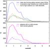 |
Fig. 11 Redshift distribution of different (not overlapping) populations, as indicated in the panels. |
7. Final counterpart catalog
The VLA-COSMOS 3 GHz Large Project multiwavelength counterpart catalog will be made available through the COSMOS IPAC/IRSA database20. This catalog is constructed in such a way that any user can easily retrieve our classification or adjust it to a different set of selection criteria. The catalog lists the counterpart IDs, properties, and the individual criteria used in this work to classify our radio sources as follows:
-
1.
Identification number of the radio source (ID_VLA).
-
2.
Right ascension (J2000) of the radio source.
-
3.
Declination (J2000) of the radio source.
-
4.
Identifier for a single- or multicomponent radio source (MULTI = 0 or 1 for the first or latter, respectively).
-
5.
Identification of the counterpart catalog, either “COSMOS2015”, “iband”, or “IRAC”.
-
6.
Identification number of the counterpart (ID_CPT).
-
7.
Right ascension (J2000) of the counterpart, corrected for small astrometry offsets as described in the Appendix.
-
8.
Declination (J2000) of the counterpart, corrected for small astrometry offsets as described in the Appendix.
-
9.
Separation between the radio source and its counterpart [arcseconds].
-
10.
False match probability.
-
11.
Best redshift available for the source.
-
12.
Integrated 3 GHz radio flux density [μJy].
-
13.
Rest-frame 3 GHz radio luminosity [log W Hz-1].
-
14.
Rest-frame 1.4 GHz radio luminosity [log W Hz-1], which is obtained using the measured 1.4–3 GHz spectral index, if available, otherwise assuming a spectral index of –0.7.
-
15.
Star formation related infrared (8–1000μm rest-frame) luminosity derived from SED fitting [log L⊙]. If the source is classified as HLAGN, this value represents the fraction of the total infrared luminosity arising from star formation, while it corresponds to the total IR luminosity otherwise (see Delvecchio et al. 2017).
-
16.
Star formation rate [M⊙yr-1] obtained from the total infrared luminosity listed in Col. (15), by assuming the Kennicutt (1998) conversion factor, and scaled to a Chabrier (2003) IMF.
-
17.
X-ray AGN: “T” if true, “F” otherwise.
-
18.
MIR AGN: “T” if true, “F” otherwise.
-
19.
SED AGN: “T” if true, “F” otherwise.
-
20.
Quiescent MLAGN: “T” if true, “F” otherwise.
-
21.
SFG: “T” if true, “F” otherwise.
-
22.
Clean SFG: “T” if true, “F” otherwise.
-
23.
HLAGN: “T” if true, “F” otherwise.
-
24.
MLAGN: “T” if true, “F” otherwise.
-
25.
Radio excess: “T” if true, “F” otherwise.
-
26.
COSMOS2015 masked area flag: “1” if true, “0” otherwise21.
The counterpart catalog presented here contains the full list of optical-MIR counterparts collected over the largest unmasked area accessible to each catalog, which is 1.77, 1.73, and 2.35 deg2 for COSMOS2015, i band, and IRAC catalogs, respectively. Complete, nonoverlapping samples within a well-defined, effective area of 1.77 square degrees; COSMOS2015 masked area flag = 0, can be formed by combining either HLAGN, MLAGN, and clean SFG samples, or alternatively the radio excess and no radio excess samples (see previous section).
8. Composition of the microJansky radio source population
In this section we analyze the composition of the faint radio population at microJansky levels. We consider nonoverlapping subsamples of the total sample of radio sources with counterparts in the COSMOS2015 or i band catalogs, defined in two different ways as described the previous sections (for a summary see Sect. 6.4 and Fig. 10). The first is based on multiwavelength criteria as follows:
-
i)
moderate-to-high radiative luminosity AGN (HLAGN;selected via X-ray-, IR-, and SED-based critera);
-
ii)
low-to-moderate radiative luminosity AGN (MLAGN; consisting of two subsamples not identified as AGN by the X-ray, IR, or SED criteria, i.e., AGN hosted by red quiescent galaxies, and those showing a >3σ excess in radio emission relative to the IR-based SFRs in their host galaxies); and
-
iii)
clean SFG sample (i.e., rest-frame color-selected SFGs that are not identified by the X-ray, IR, or SED criteria and with radio excess sources excluded; below this is often referred to as the SFG sample).
The second definition is based on radio criteria; samples of galaxies include those i) with radio excess; and ii) without radio excess, which is defined as a >3σ excess in the redshift-dependent distribution of log (L1.4 GHz/SFRIR).
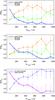 |
Fig. 12 Fractional contributions of the various populations (indicated in the panels) as a function of 3 GHz flux (top panel) and 1.4 GHz flux (middle and bottom panels). |
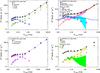 |
Fig. 13 VLA-COSMOS 3 GHz Large Project radio source counts, separated into various (not overlapping) populations (symbols, as indicated in the panels). The lines in the left panels connect the VLA-COSMOS 3 GHz Large project symbols. Lines and colored areas in the right hand-side panels show various source counts from the literature, as indicated in each panel. |
8.1. Fractional contribution of the various populations at faint radio fluxes
In the top panel of Fig. 12 we show the fractional contributions of the various populations as a function of total 3 GHz flux (S3 GHz). Dividing the populations into clean SFG, MLAGN, and HLAGN samples we find that the fraction of MLAGN decreases from about 75% at S3 GHz ~ 400–800μJy down to about 50% at S3 GHz ~ 100–400μJy and further to about 20% in our faintest flux bin at S3 GHz ~ 50 μJy. Through the same flux ranges, the fraction of SFGs increases from about 10% (S3 GHz ~ 400–800μJy) to 60% (S3 GHz ~ 50 μJy), while that of HLAGN remains fairly constant in the range of 20–30%. Hence, while the combined AGN sample (MLAGN and HLAGN) dominates the radio population at S3 GHz ≳ 100 μJy, it is the SFGs that form the bulk (60%) of the population at S3 GHz ~ 50 μJy. For easier comparison with literature, in the middle panel of Fig. 12 we show the fractional contributions of the various populations as a function of total 1.4 GHz flux, which is computed using the 1.4 GHz detections where available and assuming a spectral index of −0.7 otherwise (see Smolčić et al. 2017a, for details). The results are consistent with those described above. We find that only in our lowest flux bin (S1.4 GHz ~ 20–100μJy) the SFGs start dominating reaching a fraction of ~ 60% at S1.4 GHz ~ 50 μJy. This is consistent with the results based on the E-CDFS survey (Bonzini et al. 2013; see also below), yielding that the fraction of their SFGs is 50–60% within S1.4 GHz ~ 35–100μJy. Within the total range of S1.4 GHz ~ 20–700μJy we find a median fraction of about 40%, 30%, and 30% of MLAGN, HLAGN, and SFGs, respectively, which is in good agreement with the results based on the 1.4 GHz VLA-COSMOS survey (Smolčić et al. 2008).
As detailed in Sect. 6, the radio emission of ~ 70% of HLAGN is consistent with that expected from the star formation in their host galaxies (inferred from their IR emission). Hence, to set limits on the fractional contribution to the faint radio population by the star formation or AGN-related processes in the radio band, in the bottom panel of Fig. 12 we show the separation of all of our sources into those that show (>3σ) radio excess, and those with no radio excess relative to the SFR of the host (see Fig. 7). Consistent with the above conclusions, we find that the fraction of sources with total radio luminosity consistent with that expected from the star formation in their host galaxies increases with decreasing flux density from about 10% at S1.4 GHz ~ 700–1000μJy to ~ 85% at S1.4 GHz ~ 50 μJy, while it correspondingly decreases (from ~ 90% to ~ 15%) for sources showing significant (>3σ) radio excess. The switch between the domination of the two such selected populations occurs at S1.4 GHz ~ 200 μJy.
In conclusion, the data used here probe the flux range of the faint radio population where a switch between the dominant AGN- or star formation-related contributions occurs. This is studied further in the context of radio source counts in the next section.
8.2. Euclidean-normalized radio source counts
In Fig. 13, we show the 1.4 GHz source counts, normalized to Euclidean space, for all radio sources with counterparts in COSMOS2015 or i band catalogs and for each source class separately. The counts, tabulated in Table 2, have been corrected for completeness as described in Smolčić et al. (2017a), assuming all populations are equally complete at the same 3 GHz flux. From the left-hand panels in Fig. 13, showing the counts separated into clean SFG, MLAGN, and HLAGN in the top panel and radio excess and no radio excess samples in the bottom panel, it is obvious that galaxies with star formation activity start dominating the counts below S1.4 GHz ~ 100–150μJy, while at higher fluxes the dominating population is related to AGN activity (see also top right panel for the combined MLAGN and HLAGN contribution to the counts).
8.2.1. Comparison with radio source counts in the E-CDFS survey
In the right-hand panels of Fig. 13 we compare our Euclidean-normalized source counts to those from Padovani et al. (2015). These authors calculated the counts from 1.4 GHz VLA observations of the E-CDFS, and in the figure the color-shaded areas correspond to their counts within the reported errors (Table 1 in Padovani et al. 2015). Their sample reaches a flux density limit of 32 μJy and covers an area of approximately 0.3 deg2. Bonzini et al. (2013) separated the ~ 800 (z ≤ 4) radio sources within the E-CDFS into radio-loud (RL), radio-quiet (RQ) AGN, and SFGs using the observed 24 μm-to-1.4 GHz flux ratio (q24,obs). These authors identified RL AGN if, at a given redshift, they lay below the 2σ deviation from the average q24,obs, while they selected RQ AGN if they were above the 2σ deviation and, at the same time, fulfilled either X-ray or MIR diagnostics (similar to those used here)22. The remainder of the sample was taken as SFGs. Thus, while their classificiation scheme is largely similar to ours, it also contains significant differences. Delvecchio et al. (2017, their Sect. 4.3.2.) have provided a detailed comparison of the two classification schemes.
In the top right panel of Fig. 13 we compare our SFG, and total AGN (MLAGN and HLAGN combined) counts with the SFG and total AGN (RQ and RL combined) counts from Padovani et al. (2015), respectively. The counts show similar trends with a consistent flux of S1.4 GHz ~ 100μJy below which the dominant population switches from AGN to SFGs. While the SFG counts are consistent within the errors, the E-CDFS AGN counts show a slightly lower normalization throughout the observed range. This could be due to cosmic variance given the smaller, 0.3 deg2 E-CDFS area compared to the 2 deg2 COSMOS field area.
In the bottom right panel of Fig. 13 we compare our MLAGN and HLAGN counts with the RL and RQ AGN counts from Padovani et al. (2015). Owing to the similarity of the AGN selection methods used here and by Bonzini et al. (2013), our MLAGN (HLAGN) are expected to be a population comparable to the E-CDFS RL (RQ) AGN. The trends of our MLAGN and the E-CDFS RL AGN populations are in agreement. However, while agreement also exists between the trends of our HLAGN and E-CDFS RQ AGN at S1.4 GHz< 200 μJy, a discrepancy at higher fluxes is discernible with systematically lower count values for the E-CDFS RQ AGN. This can be understood given the differences in the selections of E-CDFS RQ AGN and our HLAGN. While the first do not contain sources with radio excess (defined by Bonzini et al. 2013 as >2σ in the redshift-dependent q24,obs, and using an M 82 galaxy template), our sample of HLAGN contains 30% of radio excess sources defined as >3σ in the redshift-dependent distribution of log (L1.4 GHz/SFRIR). Furthermore, the fraction of radio excess sources in our HLAGN sample increases with increasing flux reaching ~ 50–100% at S3 GHz ~ 0.1–1 mJy (corresponding to S1.4 GHz ~ 0.17–1.7 mJy assuming a spectral index of −0.7; see Fig. 8). Hence, the radio excess sources within our HLAGN sample could explain the higher counts of our HLAGN relative to the E-CDFS RQ AGN at S1.4 GHz> 0.2 mJy.
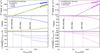 |
Fig. 14 Top panels: VLA-COSMOS 3 GHz Large Project radio source counts at S1.4 GHz< 80 μJy for various, nonoverlapping galaxy populations (symbols, as indicated in the top panels). Simple linear extrapolations (fit to the S1.4 GHz< 80 μJy data) are shown as lines. Middle panels: fractional contribution of the various populations as a function of 1.4 GHz flux, extrapolated down to the 5σ detection limits of the SKA1 Ultra Deep, Deep, and Wide radio continuum surveys (vertical dashed lines; cf. Table 1 in Prandoni & Seymour 2015). Bottom panels: cumulative fractions of clean SFGs (left), and no radio excess sources (right) as a function of 1.4 GHz flux for each of the three SKA1 flux limits (shown as the three curves in each panel). For each given flux the y-axis value corresponds to the total fraction of the population within the flux range limited at the low end by the 5σ limit of the corresponding SKA1 survey and at the high end by the flux value given on the x-axis. |
8.2.2. Comparison with the SKADS semi-empirical simulation
In the top right panel of Fig. 13, we compare our source counts for populations of SFGs and AGN with the results of the semi-empirical simulations from Wilman et al. (2008). These simulations are based on observed (or extrapolated) luminosity functions taking into account the measured large-scale clustering. Wilman et al. (2008) simulate classical radio-quiet quasars, FRI, and FRII sources, star-forming, and starburst galaxies. Since their classification is fundamentally different from ours, we only compare the total number of AGN and SFGs. We consider radio-quiet quasars, FRI, and FRII sources defined by Wilman et al. (2008) to be AGN and compare the sum of their counts to the sum of our HLAGN and MLAGN counts. The overall agreement between the two AGN counts is good, even if the Wilman et al. (2008) predictions are a bit lower than our AGN counts at flux densities below ~ 500 μJy; this is probably due to different population definitions, but is also consistent with the overall trend of their lower SKADS simulation counts compared to ours. We consider the collective sample of star-forming and starburst galaxies defined by Wilman et al. (2008) to be SFGs and compare the sum of their counts to the counts of our clean SFG sample. The prediction of Wilman et al. (2008) follows the shape of our observed SFG counts below ~ 200 μJy.
8.3. Expectations for future surveys based on simple extrapolations
In Fig. 14 we show the faint end of our source counts with two different definitions for nonoverlapping populations (left and right panels) and extrapolations down to radio fluxes of ~10 nJy, encompassing the detection limits of SKA1 Ultra Deep, Deep, and Wide surveys (Prandoni & Seymour 2015). In a zero-order attempt to extrapolate the counts, not intended to be related to any physical model, we use a simple linear fit to the four faintest data points (S1.4 GHz< 80 μJy) for each of the various radio-detected subpopulations. As discernible from the middle panels in the figure, down to these fluxes the expected fractions of MLAGN and HLAGN (radio excess sources) drop monotonously, while that of SFGs (no radio excess sources) monotonously rises toward unity. In the bottom panels of Fig. 14 we show the cumulative fractions of clean SFGs and no radio excess sources as a function of 1.4 GHz flux for each of the three SKA1 flux limits. This was computed as the total fraction of the population within the flux range limited at the low end by the 5σ limit of the corresponding SKA1 survey and at the high end by the given flux value. For example, selecting radio-detected sources with S1.4 GHz< 80 μJy (corresponding to S3 GHz< 48 μJy, assuming α = −0.7) yields a sample that consists of about 72%, 83%, and 89% SFGs in the planned SKA1 Wide, Deep, and Ultra Deep surveys, respectively. Selecting sources with S1.4 GHz< 10 μJy (corresponding to S3 GHz< 6 μJy, assuming α = −0.7) results in samples that consist of about 76%, 83%, and 89% SFGs in the three SKA1 surveys, respectively. Considering only objects with no radio excess these numbers are about 92%, 97%, and 99% and 96%, 98%, and 99% for upper flux limits of 80 and 10 μJy, respectively. Hence, it can be expected that at the faint flux limits to be reached by the SKA1 surveys, a selection based only on radio flux limits can provide a simple tool to identify efficiently samples highly dominated by SFGs.
9. Summary
Using one of the deepest radio data sets so far, the VLA-COSMOS 3 GHz Large Project, down to a flux limit of ~11 μJy at 5σ, we associated optical/NIR/MIR counterparts to radio sources. Counterpart candidates were drawn from three different catalogs: COSMOS2015, i band, and IRAC, prioritizing them in that order. A false match probability was calculated for each counterpart candidate using a background model designed to reproduce realistic magnitude and spatial distribution of counterparts to radio sources. We select as reliable counterparts those counterpart candidates with false match probability below 20% in at least one of the three catalogs. In total, we find 8035 counterparts to our 3 GHz radio sources over a common unmasked area of 1.77 deg2 with an estimated fraction of spurious identifications of ~ 2%.
We analyzed the multiwavelength star formation- and AGN-related properties of our radio-selected population, reaching out to a redshift of z ~ 6. Based on the multiwavelength properties, including the estimated bolometric (i.e., radiative) AGN luminosities, we separate our radio sources into subsamples of clean SFGs and those of radio AGN into low-to-moderate and moderate-to-high radiative luminosity radio AGN; we consider these AGN subpopulations to be candidates for high-redshift analogs to local low- and high-excitation emission line AGN, respectively. An alternative separation is that into subsamples of galaxies with and without radio excess, where the radio excess threshold is defined as a 3σ excess in radio emission relative to the IR-based SFRs in their host galaxies.
An analysis of fractional contributions of various galaxy types as a function of radio flux shows that below ~100 μJy at 1.4 GHz star-forming (no radio excess) galaxies constitute the dominant fraction of the radio population with a ~ 60% (80%) contribution at S1.4 GHz ~ 50 μJy. At higher flux density levels the fractional contribution of star-forming (no radio excess) galaxies diminishes and AGN (radio excess galaxies) constitute the dominant fraction.
The Euclidean normalized number counts of different observed populations are generally in agreement with the number counts of similar observed or simulated populations from the literature. Using simple extrapolations of our faint-end (S1.4 GHz< 80 μJy) counts we estimate the differential and cumulative fractions of SFGs and galaxies with no radio excess. These suggest that at the faint flux limits the planned (Wide, Deep, and UltraDeep) SKA1 surveys will reach, a selection based only on radio flux limits can provide a simple tool to identify efficiently samples highly dominated by SFGs.
The primary beam half-power beam width is a function of frequency and varies by a factor of 2 between the lower and upper frequency edge of the S band. At 3 GHz frequency it corresponds to 15′ allowing coverage of a 2 square degree field with ~ 64 pointings.
For a typical spectral index of α = −0.7 the flux density at 3 GHz observing frequency (S band) is a factor of 1.67 lower than at 1.4 GHz observing frequency (L band). Assuming an effective bandwidth of 1.664 GHz in the S band, and 400–600 MHz in the L band to reach an rms of 2.3 μJy/beam at 3 GHz observing frequency, which is equivalent to an rms of 3.9μJy/beam at 1.4 GHz observing frequency for α = −0.7 requires per pointing a factor of about 1.4–1.9 more observing time in the L band compared to the S band. On the other hand, to reach a uniform rms over a 2 square degree field 23 pointings are required in the L band, while 64 are required in the S band. This contributes to a slightly higher overhead time in the S band owing to longer telescope slewing times. Also, the S band offers further advantages over the L band, such as a (factor of ~ 2) higher angular resolution and the large bandwidth, which can simultaneously provide spectral shape information for bright sources in the field.
The observations of the COSMOS field in the z band were performed with Subaru Suprime-Cam (Taniguchi et al. 2007, 2015). The initial COSMOS z band (z+) data are superseded by deeper z band observations obtained with upgraded CCDs and a different filter (z++). Data in YJHKS bands refer to that obtained by the Ultra Deep Survey with the VISTA telescope (see also Laigle et al. 2016).
Normalized median absolute deviation (Hoaglin et al. 1983) defined as 1.48 times the median value of | zphot−zspec | /(1 + zspec).
The DEIMOS data were taken from various independent observational campaigns led by Nick Scoville, Peter Capak, David Sanders, Guenther Hasinger, Jeyhan Kartaltepe, Mara Salvato, and Caitlin Casey.
7681 and 48 single- and multicomponent sources, respectively.
97 and 0 single- and multicomponent sources, respectively.
209 and 0 single- and multicomponent sources, respectively.
The reliability of each spectroscopic redshift relies on the corresponding quality flag. In case of spectroscopic redshift from the zCOSMOS survey (Lilly et al. 2007, 2009), we followed the prescription recommended in the zCOSMOS IRSA webpage: https://irsa.ipac.caltech.edu/data/COSMOS/spectra/z-cosmos/Z-COSMOS_INFO.html. For the other surveys we selected spectroscopic redshifts with quality flag Qf ≥ 3 and discarded less reliable measurements from our analysis.
A total of 4879 radio sources are detected within 1.77 deg2 at ≥3σ in at least one Herschel band, which are associated with optical/NIR counterparts from either the COSMOS2015 catalog (4836) or the i band selected catalog (43). For about 100 radio sources (sub-)millimetre data was also available within  of optical/NIR positions (see Sect. 2.3).
Consistent with the nomenclature used in Delvecchio et al. (2017).
This flag was computed for the counterpart positions against the COSMOS2015 mosaics indicating the masked areas and agrees to 0.17% with the masked areas reported in the COSMOS2015 catalog.
Note that the q24,obs ratio is defined in an inverse manner compared to the log (L1.4 GHz/SFRIR) ratio used here.
The association is constructed in such a way that the COSMOS2015 sources listed can have IRAC and/or i band counterparts, while the i band sources listed can have IRAC counterparts, but do not have unmasked COSMOS2015 counterparts and the IRAC sources listed do not have unmasked COSMO2015 nor i band counterparts.
Acknowledgments
Zgal group: European Union’s Seventh Framework program under grant agreement 333654 (CIG, “AGN feedback”; N.B., V.S.) and grant agreement 337595 (ERC Starting Grant, “CoSMass”; V.S., I.D., J.D., M.N.). C.L. acknowledges the funding by a Discovery Early Career Researcher Award (DE150100618). Partially based on data obtained with the European Southern Observatory Very Large Telescope, Paranal, Chile, under Large Programs 175.A-0839 (the zCOSMOS Spectroscopic Redshift Survey) and 185.A-0791 (the VIMOS Ultra Deep Survey). A.K. and E.V. acknowledge support from the collaborative research center 956 (sub-project A1) funded by the Deutsche Forschungsgemeinschaft (DFG).
References
- Afonso, J., Georgakakis, A., Almeida, C., et al. 2005, ApJ, 624, 135 [NASA ADS] [CrossRef] [Google Scholar]
- Allen, S. W., Dunn, R. J. H., Fabian, A. C., Taylor, G. B., & Reynolds, C. S. 2006, MNRAS, 372, 21 [NASA ADS] [CrossRef] [Google Scholar]
- Aretxaga, I., Wilson, G. W., Aguilar, E., et al. 2011, MNRAS, 415, 3831 [NASA ADS] [CrossRef] [Google Scholar]
- Arnouts, S., Cristiani, S., Moscardini, L., et al. 1999, MNRAS, 310, 540 [NASA ADS] [CrossRef] [Google Scholar]
- Berta, S., Lutz, D., Santini, P., et al. 2013, A&A, 551, A100 [NASA ADS] [CrossRef] [EDP Sciences] [Google Scholar]
- Bertoldi, F., Carilli, C., Aravena, M., et al. 2007, ApJS, 172, 132 [NASA ADS] [CrossRef] [Google Scholar]
- Best, P. N., Kaiser, C. R., Heckman, T. M., & Kauffmann, G. 2006, MNRAS, 368, L67 [NASA ADS] [Google Scholar]
- Bonzini, M., Padovani, P., Mainieri, V., et al. 2013, MNRAS, 436, 3759 [NASA ADS] [CrossRef] [Google Scholar]
- Burbidge, G. R. 1956, ApJ, 124, 416 [NASA ADS] [CrossRef] [Google Scholar]
- Calistro Rivera, G., Williams, W. L., Hardcastle, M. J., et al. 2017, MNRAS, submitted [arXiv:1704.06268] [Google Scholar]
- Capak, P., Aussel, H., Ajiki, M., et al. 2007, ApJS, 172, 99 [NASA ADS] [CrossRef] [Google Scholar]
- Casey, C. M., Chen, C.-C., Cowie, L. L., et al. 2013, MNRAS, 436, 1919 [NASA ADS] [CrossRef] [Google Scholar]
- Chabrier, G. 2003, ApJ, 586, L133 [NASA ADS] [CrossRef] [Google Scholar]
- Civano, F., Marchesi, S., Comastri, A., et al. 2016, ApJ, 819, 62 [NASA ADS] [CrossRef] [Google Scholar]
- Condon, J. J. 1992, ARA&A, 30, 575 [NASA ADS] [CrossRef] [MathSciNet] [Google Scholar]
- Cowie, L. L., Barger, A. J., Fomalont, E. B., & Capak, P. 2004, ApJ, 603, L69 [NASA ADS] [CrossRef] [Google Scholar]
- da Cunha, E., Charlot, S., & Elbaz, D. 2008, MNRAS, 388, 1595 [NASA ADS] [CrossRef] [Google Scholar]
- Delhaize, J., Smolcic, V., Delvecchio, I., et al. 2017, A&A, 602, A4 (VLA-COSMOS SI) [NASA ADS] [CrossRef] [EDP Sciences] [Google Scholar]
- Delvecchio, I., Gruppioni, C., Pozzi, F., et al. 2014, MNRAS, 439, 2736 [NASA ADS] [CrossRef] [Google Scholar]
- Delvecchio, I., Smolcic, V., Zamorani, G., et al. 2017, A&A, 602, A3 (VLA-COSMOS SI) [NASA ADS] [CrossRef] [EDP Sciences] [Google Scholar]
- Donley, J. L., Koekemoer, A. M., Brusa, M., et al. 2012, ApJ, 748, 142 [NASA ADS] [CrossRef] [Google Scholar]
- Donoso, E., O’Mill, A., & Lambas, D. G. 2006, MNRAS, 369, 479 [NASA ADS] [CrossRef] [Google Scholar]
- Elvis, M., Civano, F., Vignali, C., et al. 2009, ApJS, 184, 158 [NASA ADS] [CrossRef] [Google Scholar]
- Evans, D. A., Worrall, D. M., Hardcastle, M. J., Kraft, R. P., & Birkinshaw, M. 2006, ApJ, 642, 96 [NASA ADS] [CrossRef] [Google Scholar]
- Feltre, A., Hatziminaoglou, E., Fritz, J., & Franceschini, A. 2012, MNRAS, 426, 120 [NASA ADS] [CrossRef] [Google Scholar]
- Fritz, J., Franceschini, A., & Hatziminaoglou, E. 2006, MNRAS, 366, 767 [Google Scholar]
- Georgakakis, A., Mobasher, B., Cram, L., et al. 1999, MNRAS, 306, 708 [NASA ADS] [CrossRef] [Google Scholar]
- Griffin, M. J., Abergel, A., Abreu, A., et al. 2010, A&A, 518, L3 [Google Scholar]
- Gruppioni, C., Mignoli, M., & Zamorani, G. 1999, MNRAS, 304, 199 [NASA ADS] [CrossRef] [Google Scholar]
- Hardcastle, M. J., Kraft, R. P., & Worrall, D. M. 2006, MNRAS, 368, L15 [NASA ADS] [CrossRef] [Google Scholar]
- Hardcastle, M. J., Kraft, R. P., Worrall, D. M., et al. 2007, ApJ, 662, 166 [NASA ADS] [CrossRef] [Google Scholar]
- Hardcastle, M. J., Ching, J. H. Y., Virdee, J. S., et al. 2013, MNRAS, 429, 2407 [NASA ADS] [CrossRef] [Google Scholar]
- Heckman, T. M., & Best, P. N. 2014, ARA&A, 52, 589 [Google Scholar]
- Hine, R. G., & Longair, M. S. 1979, MNRAS, 188, 111 [NASA ADS] [Google Scholar]
- Hoaglin, D. C., Mosteller, F., & Tukey, J. W. 1983, Understanding robust and exploratory data analysis (New York: Wiley) [Google Scholar]
- Hughes, A. M., Beasley, A., & Carilli, C. 2015, IAU General Assembly, 22, 2255106 [NASA ADS] [Google Scholar]
- Huynh, M. T., Jackson, C. A., Norris, R. P., & Prandoni, I. 2005, AJ, 130, 1373 [NASA ADS] [CrossRef] [Google Scholar]
- Ilbert, O., Arnouts, S., McCracken, H. J., et al. 2006, A&A, 457, 841 [NASA ADS] [CrossRef] [EDP Sciences] [Google Scholar]
- Ilbert, O., Capak, P., Salvato, M., et al. 2009, ApJ, 690, 1236 [NASA ADS] [CrossRef] [Google Scholar]
- Ilbert, O., Salvato, M., Le Floc’h, E., et al. 2010, ApJ, 709, 644 [NASA ADS] [CrossRef] [Google Scholar]
- Ilbert, O., McCracken, H. J., Le Fèvre, O., et al. 2013, A&A, 556, A55 [NASA ADS] [CrossRef] [EDP Sciences] [Google Scholar]
- Jarvis, M. J., & Rawlings, S. 2004, New Astron. Rev., 48, 1173 [NASA ADS] [CrossRef] [Google Scholar]
- Karim, A., Schinnerer, E., Martínez-Sansigre, A., et al. 2011, ApJ, 730, 61 [NASA ADS] [CrossRef] [Google Scholar]
- Kennicutt, Jr., R. C. 1998, ApJ, 498, 541 [NASA ADS] [CrossRef] [Google Scholar]
- Kriek, M., Shapley, A. E., Reddy, N. A., et al. 2015, ApJS, 218, 15 [NASA ADS] [CrossRef] [Google Scholar]
- Laigle, C., McCracken, H. J., Ilbert, O., et al. 2016, ApJS, 224, 24 [NASA ADS] [CrossRef] [Google Scholar]
- Laing, R. A., Jenkins, C. R., Wall, J. V., & Unger, S. W. 1994, in The Physics of Active Galaxies, eds. G. V. Bicknell, M. A. Dopita, & P. J. Quinn, ASP Conf. Ser., 54, 201 [Google Scholar]
- Lanzuisi, G., Perna, M., Delvecchio, I., et al. 2015, A&A, 578, A120 [NASA ADS] [CrossRef] [EDP Sciences] [Google Scholar]
- Le Fèvre, O., Tasca, L. A. M., Cassata, P., et al. 2015, A&A, 576, A79 [NASA ADS] [CrossRef] [EDP Sciences] [Google Scholar]
- Le Floc’h, E., Aussel, H., Ilbert, O., et al. 2009, ApJ, 703, 222 [NASA ADS] [CrossRef] [Google Scholar]
- Lilly, S. J., Le Fèvre, O., Renzini, A., et al. 2007, ApJS, 172, 70 [NASA ADS] [CrossRef] [Google Scholar]
- Lilly, S. J., Le Brun, V., Maier, C., et al. 2009, ApJS, 184, 218 [Google Scholar]
- Lutz, D., Poglitsch, A., Altieri, B., et al. 2011, A&A, 532, A90 [NASA ADS] [CrossRef] [EDP Sciences] [Google Scholar]
- Magnelli, B., Ivison, R. J., Lutz, D., et al. 2015, A&A, 573, A45 [NASA ADS] [CrossRef] [EDP Sciences] [Google Scholar]
- Marchesi, S., Civano, F., Elvis, M., et al. 2016, ApJ, 817, 34 [NASA ADS] [CrossRef] [Google Scholar]
- Miettinen, O., Smolčić, V., Novak, M., et al. 2015, A&A, 577, A29 [NASA ADS] [CrossRef] [EDP Sciences] [Google Scholar]
- Miley, G. 1980, ARA&A, 18, 165 [Google Scholar]
- Norris, R. P., Afonso, J., Bacon, D., et al. 2013, PASA, 30, e020 [NASA ADS] [CrossRef] [Google Scholar]
- Novak, M., Smolcic, V., Delhaize, J., et al. 2017, A&A, 602, A5 (VLA-COSMOS SI) [NASA ADS] [CrossRef] [EDP Sciences] [Google Scholar]
- Oliver, S. J., Bock, J., Altieri, B., et al. 2012, MNRAS, 424, 1614 [NASA ADS] [CrossRef] [EDP Sciences] [Google Scholar]
- Padovani, P. 2016, A&ARv, 24, 13 [NASA ADS] [CrossRef] [Google Scholar]
- Padovani, P., Bonzini, M., Kellermann, K. I., et al. 2015, MNRAS, 452, 1263 [Google Scholar]
- Poglitsch, A., Waelkens, C., Geis, N., et al. 2010, A&A, 518, L2 [NASA ADS] [CrossRef] [EDP Sciences] [Google Scholar]
- Prandoni, I., & Seymour, N. 2015, in Proc. Advancing Astrophysics with the Square Kilometre Array (AASKA14), 67 [Google Scholar]
- Sadler, E. M., Jenkins, C. R., & Kotanyi, C. G. 1989, MNRAS, 240, 591 [NASA ADS] [Google Scholar]
- Sadler, E. M., Ekers, R. D., Mahony, E. K., Mauch, T., & Murphy, T. 2014, MNRAS, 438, 796 [NASA ADS] [CrossRef] [Google Scholar]
- Salvato, M., Hasinger, G., Ilbert, O., et al. 2009, ApJ, 690, 1250 [CrossRef] [Google Scholar]
- Salvato, M., Ilbert, O., Hasinger, G., et al. 2011, ApJ, 742, 61 [NASA ADS] [CrossRef] [Google Scholar]
- Sanders, D. B., Salvato, M., Aussel, H., et al. 2007, ApJS, 172, 86 [Google Scholar]
- Schinnerer, E., Carilli, C. L., Scoville, N. Z., et al. 2004, AJ, 128, 1974 [NASA ADS] [CrossRef] [Google Scholar]
- Schinnerer, E., Smolčić, V., Carilli, C. L., et al. 2007, ApJS, 172, 46 [NASA ADS] [CrossRef] [Google Scholar]
- Schinnerer, E., Sargent, M. T., Bondi, M., et al. 2010, ApJS, 188, 384 [NASA ADS] [CrossRef] [Google Scholar]
- Schlegel, D. J., Finkbeiner, D. P., & Davis, M. 1998, ApJ, 500, 525 [NASA ADS] [CrossRef] [Google Scholar]
- Scott, K. S., Austermann, J. E., Perera, T. A., et al. 2008, MNRAS, 385, 2225 [NASA ADS] [CrossRef] [Google Scholar]
- Scoville, N., Aussel, H., Brusa, M., et al. 2007, ApJS, 172, 1 [NASA ADS] [CrossRef] [Google Scholar]
- Shakura, N. I., & Sunyaev, R. A. 1973, A&A, 24, 337 [NASA ADS] [Google Scholar]
- Simpson, C., Martínez-Sansigre, A., Rawlings, S., et al. 2006, MNRAS, 372, 741 [NASA ADS] [CrossRef] [Google Scholar]
- Smolčić, V. 2009, ApJ, 699, L43 [NASA ADS] [CrossRef] [Google Scholar]
- Smolčić, V., Schinnerer, E., Scodeggio, M., et al. 2008, ApJS, 177, 14 [NASA ADS] [CrossRef] [Google Scholar]
- Smolčić, V., Schinnerer, E., Zamorani, G., et al. 2009, ApJ, 690, 610 [NASA ADS] [CrossRef] [Google Scholar]
- Smolčić, V., Aravena, M., Navarrete, F., et al. 2012, A&A, 548, A4 [NASA ADS] [CrossRef] [EDP Sciences] [Google Scholar]
- Smolčić, V., Padovani, P., Delhaize, J., et al. 2015, in Proc. Advancing Astrophysics with the Square Kilometre Array (AASKA14), 69 [Google Scholar]
- Smolčić, V., Novak, M., Bondi, M., et al. 2017a, A&A, 602, A1 (VLA-COSMOS SI) [NASA ADS] [CrossRef] [EDP Sciences] [Google Scholar]
- Smolčić, V., Novak, M., Delvecchio, I., et al. 2017b, A&A, 602, A6 [NASA ADS] [CrossRef] [EDP Sciences] [Google Scholar]
- Symeonidis, M., Georgakakis, A., Page, M. J., et al. 2014, MNRAS, 443, 3728 [NASA ADS] [CrossRef] [Google Scholar]
- Szokoly, G. P., Bergeron, J., Hasinger, G., et al. 2004, ApJS, 155, 271 [NASA ADS] [CrossRef] [Google Scholar]
- Taniguchi, Y., Scoville, N., Murayama, T., et al. 2007, ApJS, 172, 9 [NASA ADS] [CrossRef] [Google Scholar]
- Taniguchi, Y., Kajisawa, M., Kobayashi, M. A. R., et al. 2015, PASJ, 67, 104 [NASA ADS] [Google Scholar]
- Tasca, L. A. M., Le Fevre, O., Ribeiro, B., et al. 2017, A&A, 600, 110 [Google Scholar]
- Tozzi, P., Gilli, R., Mainieri, V., et al. 2006, A&A, 451, 457 [NASA ADS] [CrossRef] [EDP Sciences] [Google Scholar]
- Wilman, R. J., Miller, L., Jarvis, M. J., et al. 2008, MNRAS, 388, 1335 [NASA ADS] [Google Scholar]
- Xue, Y. Q., Brandt, W. N., Luo, B., et al. 2010, ApJ, 720, 368 [NASA ADS] [CrossRef] [Google Scholar]
Appendix A: Associating counterparts to single-component radio sources
We here describe in detail the procedure used to associate optical-MIR counterparts with our 3 GHz, single-component radio sources.
Appendix A.1: Separation between positions of radio and optical-MIR sources
Positional matching of the VLA-COSMOS 3 GHz Large Project (Smolčić et al. 2017a) sources with those in the COSMOS2015 (Laigle et al. 2016), i band (Capak et al. 2007), and 3.6 μm IRAC (Sanders et al. 2007) selected catalogs reveals small systematic positional offsets, listed in Table A.1, which also depend on the position on the sky (see left panels of Fig. A.1). Thus, prior to associating optical-MIR counterparts with our radio sources, we correct the multiwavelength catalog positions for these astrometric offsets via a linear fit to the mean (radio-optical, radio-NIR or radio-MIR) astrometric offsets as a function of RA and Dec (see the right panels of Fig. A.1).
The best-fit expressions to determine the corrected optical-MIR positions (RA′, Dec′) for each counterpart catalog are given below. COSMOS2015 catalog:  i band catalog:
  IRAC catalog:
 Next, to choose the limiting counterpart search radius we compare the number of radio – opt/NIR/MIR nearest neighbors of our radio sources, in the optical, NIR-, and MIR-selected catalogs, as a function of search radius with that obtained from a random position distribution. This is shown in Fig. A.3 where the number of matches with random positions is represented by the average of 10 randomizations of each of the optical, NIR-, and MIR-selected catalogs.
At small separations (<1′′) the peak in the number of matches around the positions of the radio sources is due to the large number of true counterparts. At large separations (>2′′- 3′′) the number of matches around the positions of the radio sources follows a linear relation that is consistent with that observed around random positions. The different slopes of these linear relations correspond to the different surface densities of the sources in the three different catalogs and at these separations there is no excess of counts with respect to what is observed around random positions. At intermediate separations the number of associations around the positions of the radio sources is smaller than that observed around random positions and this number reaches a minimum at separations of ~1–1.5θ, where θ is the FWHM of the PSF (θ ~ 0.̋8 for COSMOS2015/i band, and θ ~ 1.̋66 for IRAC). This deficiency in the number of matches with the radio sources, relative to the number of matches with the randomized position catalog (at r ~ 0.7–3″ for COSMOS2015 and the i band selected catalogs, spanning up to 4′′ for the IRAC catalog) is because fainter optical/NIR/MIR sources close to the brighter counterparts of radio sources (see Fig. A.2) at smaller separations cannot be easily detected and most of these sources are therefore missing in the catalogs (i.e., a blocking effect). Although Fig. A.3 appears to suggest, at face value, that most of the counterparts between 0.̋4 and 0.̋8 are not associated with radio sources, the magnitude distribution of these counterparts as a function of separation suggests instead that many of those sources, especially the brightest, are real associations, as is discussed in the next section.
Mean offsets in RA and Dec separations for sources matched between the VLA-COSMOS 3 GHz Large Project catalog and the COSMOS2015, i band, and IRAC 3.6 μm selected catalogs.
 |
Fig. A.1 Systematic positional offsets in the (RA, Dec) plane between the VLA-COSMOS 3 GHz Large Project and the COSMOS2015 (top panels), i band (middle panels), and IRAC (bottom panels) sources before (left panels) and after corrections (right panels). To obtain the corrections the 1.4° × 1.4° COSMOS field was divided into 100 bins 0.14° on the side. In each bin, a Gaussian was fitted to the separation distribution in right ascension and declination. The means of these two Gaussians are shown as the vectors shown in the plot. For visibility, the sizes of the vectors are multiplied by a factor 3600. |
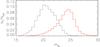 |
Fig. A.2 Normalized KS magnitude distribution of 3 GHz source counterpart candidates from the COSMOS2015 catalog (black), and all sources in the unmasked regions of COSMOS2015 with KS band detection (red). The magnitudes are formal (positive flux) values derived at the position of objects identified in the z++YJHKs stack. |
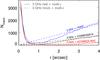 |
Fig. A.3 Number of all matches within 0.1″ wide annuli between the VLA-COSMOS 3 GHz Large Project sources and the COSMOS2015 (black), the i band selected (blue), and the IRAC 3.6 μm selected catalogs (red) (solid lines). Dashed lines represent the average number of matches in the three above-mentioned catalogs around randomized positions. The average was calculated using 10 different randomizations. |
Appendix A.2: False match probability
To estimate the reliability of the radio-optical/NIR/MIR matches and the false match probability (pfalse), we created a background model that reproduces the blocking effect of optical, NIR, and MIR sources around radio sources. To simulate the i band and IRAC background, their selection band was used (i and 3.6 μm respectively), while for the COSMOS2015 background model the 3.6 μm band, measured for a large majority of the sources, was chosen. First, we divide each sample of N counterpart candidates (COSMOS2015, i band, and IRAC) into N = Nm + Nu, where Nm (Nu) is the number of closest counterparts found within 0.5θ (⟨ 0.5,1.5 ] θ) from the radio source position. For all three catalogs Nm and Nu are ~85–90% and ~10–15% of N, respectively. As said above, it is this large number of relatively bright counterparts close to the radio positions that artificially reduces the number of sources in the optical, NIR, and MIR catalogs at separations larger than 0.5θ. To reproduce this effect, from each catalog we select Nm sources and require them to follow the magnitude distribution of real counterparts matched using a 0.5θ search radius; then, starting from the positions of these randomly selected sources, we set the center of our search region by moving it in a random direction following the separation distribution of real counterpart candidates matched using a 0.5θ search radius. Thus, we simulate Nm sources whose magnitudes and separations fully reflect those of the real sample of counterparts within the 0.5θ search radius. Finally, we randomly distribute the remaining Nu sources over the entire radio field. We generate 100 different mock (background) catalogs following this recipe and extract the expected background magnitude distribution from the counterparts to these mock sources.
The false match probability as a function of magnitude was then calculated in two separation bins as the ratio between the distributions of the simulated background and real magnitudes. We then linearly interpolate the histogram of this ratio and assign to each source the false match probability that this interpolation has at the value of the magnitude of the source. This is illustrated in Fig. A.4 and summarized in Fig. A.5. Details on matching with the COSMOS2015, i band, and IRAC sources, as well as the false match probability estimation, are given in the following sections. False match probabilities were not calculated and their values were set to 1 for sources without the measured magnitude in the band used for the background estimation (see Sects. A.3, and A.4).
Appendix A.3: Cross-matching with the COSMOS2015 sources: NIR counterpart candidates
Masked regions of the COSMOS2015 catalog illustrated in Fig. 1 reduce the effective area to 1.77 deg2. A total of 8696 (~80%) 3 GHz sources fall within this area. COSMOS2015 sources outside the masked regions were positionally matched to the sources in the VLA-COSMOS 3 GHz Large Project catalog via a search radius of 0.̋8. Including multiple possible counterpart candidates for a single 3 GHz source, this yielded a total of 7721 COSMOS2015 counterpart candidates, and 7701 single radio-NIR source associations. Only six counterpart candidates did not have the 3.6 μm magnitude listed in the catalog and their false match probabilities were manually set to 1. Magnitude distributions and pfalse (i.e., ratio between the number of associations with the simulated mock catalogs and the number of associations with the real catalog) versus magnitude plots are shown in the top panels of Fig. A.4. The pfalse distribution of the matched sample is shown in the top panel of Fig A.5.
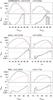 |
Fig. A.4 Top panels in each row: magnitude distribution of the real VLA-COSMOS 3 GHz counterparts (solid black line), and the simulated background (red dashed line) for the COSMOS2015 (top row), i band (middle row), and IRAC (bottom row) catalogs. The range of allowed separations between the radio sources and their counterparts is indicated above each panel (see text for details). Bottom panels in each row: ratio between the background and real magnitude distributions, defined as the false match probability (pfalse), as a function of magnitude. The dotted horizontal line shows the pfalse threshold of 0.2 beyond which counterparts are discarded, while the dotted vertical line shows the effective magnitude cut corresponding to pfalse = 0.2. Poisson errors are also indicated. |
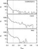 |
Fig. A.5 Distribution of the false match probability (pfalse) for the VLA 3 GHz sources matched to COSMOS2015 selected (top), i band selected sources (middle), and IRAC, 3.6 μm selected sources (bottom). The vertical dotted line shows the pfalse threshold of 20% used in the counterpart association. |
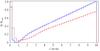 |
Fig. A.6 Normalized number of i band (IRAC) sources at a given distance from COSMOS2015 sources, shown as a blue solid (red dashed) histogram. |
Appendix A.4: Cross-matching with the i band selected sources
From the i band selected catalog (Capak et al. 2007) of 2 017 800 sources, we excluded those masked (i.e., if saturated or around bright sources) in the B, V, i, and z bands, removing 26% of the sources and leaving 1 484 453 reliable detections. A total of 8696 (~80%) 3 GHz sources fall within the unmasked regions with an effective area of 1.73 square degrees. Within a search radius of 0.̋8, we find a total of 7397 i band selected counterparts of 3 GHz sources, including multiple possible candidates for the same radio source and 7321 for a one-to-one match. For only 16 sources i band magnitudes were not available and their false match probabilities were set to 1. Magnitude distributions and false match probabilities are shown in the middle panels of Fig. A.4. The false match probability distribution of the matched sample is shown in the middle panel of Fig A.5.
Appendix A.5: Cross-matching with the IRAC selected sources
We excluded sources masked in any of the four IRAC channels from the IRAC 3.6 μm selected catalog. This reduced the number of sources from 345 512 to 278 897. Within a search radius of 1.̋7, we find 9158 3.6 μm sources in total, which are all unique IRAC-radio source matches. All the counterpart candidates have a 3.6 μm magnitude. Magnitude distributions and false match probabilities are shown in the bottom panels of Fig. A.4. The false match probability distribution of the matched sample is shown in the bottom panel of Fig A.5.
Appendix A.6: Final catalog of optical-MIR counterparts
To find the best possible multiwavelength counterpart of VLA-COSMOS 3 GHz Large Project sources, we compared the three (COSMOS2015, i band, and IRAC) counterpart candidate catalogs described in previous sections. Over 7000 single-component radio sources have a counterpart candidate in all three catalogs. To verify whether the counterpart candidates found in the three catalogs represent the same physical source we proceed in the following way. To find COSMOS2015 counterparts to i band and IRAC sources, and i band counterparts to IRAC sources, we perform positional matching between these catalogs. To determine the search radius for the association of sources appearing in two different catalogs, we count the number of sources as a function of separation as shown in Fig. A.6. As the maximum search radius, we use the radius where this number reaches the minimum: above this radius the associations are consistent with being spurious and their number, linearly increasing with separation, is simply due to the surface density of sources in the two analyzed catalogs. This radius is ~0.̋7 for the match between the COSMOS2015 and i band catalogs and 1″ for the match between the COSMOS2015 and IRAC catalogs. Thus, after selecting a reliable (i.e., one with pfalse less than 20%) counterpart in the i band and IRAC catalogs, we shift the selection to the COSMOS2015 counterpart if it is within 0.̋7 from the i band or 1″ from the IRAC counterpart but still within a separation of between the radio and COSMOS2015/i band counterpart. Similarly, we shift the selection to the i band counterpart if it is within 1″ from a reliable IRAC counterpart. Since it is unlikely that a source that is detected in two different surveys is spurious, in these cases we associate the COSMOS2015 or i band counterpart regardless of its false match probability. The total number of cases in which COSMOS2015 or i band sources with false match probability pfalse> 20% were selected was 1.1%.
Appendix B: Full 3 GHz radio source counterpart catalog
Summary of the cross-correlation of the VLA-COSMOS 3 GHz Large Project sources with sources in the multiwavelength catalogs.
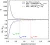 |
Fig. B.1 Differential (top panel) distribution of the separations of the final counterparts from the (single-component) radio sources, drawn from the COSMOS2015, i band, or IRAC catalogs (as described in the text). The bottom panel shows the cumulative distributions of the separations of all counterpart candidates (with pfalse ≤ 0.2) drawn from the COSMOS2015 (blue dashed curve), i band (green dotted curve), and IRAC (red dash-dotted curve) catalogs. Also indicated is the separation encompassing 99% of the counterparts for each of the counterpart sample. |
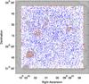 |
Fig. B.2 Positions of counterparts from COSMOS2015 (blue crosses), i band (yellow circles), and IRAC (red triangles) catalogs overlaid on the VLA-COSMOS 3 GHz Large Project mosaic with grayed-out regions masked in COSMOS2015 catalog due to the presence of saturated or bright sources in the optical to NIR bands (see also Fig 1). |
The full 3 GHz radio source counterpart catalog contains all 3 GHz sources with counterparts assigned either in the COSMOS2015, i band, or IRAC catalogs, as described in detail in Appendix A, and summarized in Sects. 3.2, 3.1, and 7. The final counterparts assigned to both our multi- and single-component 3 GHz radio sources are summarized in Table B.1.
Overall, 7742, 407, and 1012 radio (3 GHz) sources are associated with COSMOS2015, i band, and IRAC counterparts, respectively23. In total, we find 9161 counterparts for our radio sources. Summing the computed false match probabilities we estimate a total fraction of spurious matches of ~ 2%. Since our identification procedure is based on ground-based catalogs, it is likely that this “formal” fraction should be considered a lower limit because of the limited spatial resolution of these data used in these catalogs.
In the top panel of Fig. B.1 we show the differential distribution of the separations of final counterparts from the radio sources. The differential distribution is highly peaked at small separations. As evident in the cumulative distribution and separated into all counterpart candidates with pfalse ≤ 0.2 from the various catalogs, which are shown in the bottom panel, 99% of the associations are found within a separation of ~ 0.7″ (1.4″) between the 3 GHz and the COSMOS/i band (IRAC) matches. This further affirms our choice of the limiting matching distance of () for COSMOS2015/i band (IRAC). Extending the chosen limiting search radii would not have significantly increased the counterpart sample at the expense of the possible inclusion of a non-negligible fraction of spurious associations.
In Fig. B.2 we show the positions of the identified counterparts overlaid on the COSMOS field. We stress the difference in effective, unmasked regions of the maps where the three counterpart catalogs were extracted from (z++JYHK stack, i band, 3.6 μm band, respectively): 1.77 square degrees for COSMOS2015, 1.73 square degree area for the i band, and 2.35 square degree area for the IRAC catalogs. For this reason the bulk of the IRAC (79%) and i band (76%) assigned counterparts resides either in the outer regions of the field that is not covered by the COSMOS2015 catalog or in COSMOS2015 masked regions.
All Tables
Summary of the cross-correlation of the VLA-COSMOS 3 GHz Large Project sources with sources in the multiwavelength catalogs.
Mean offsets in RA and Dec separations for sources matched between the VLA-COSMOS 3 GHz Large Project catalog and the COSMOS2015, i band, and IRAC 3.6 μm selected catalogs.
Summary of the cross-correlation of the VLA-COSMOS 3 GHz Large Project sources with sources in the multiwavelength catalogs.
All Figures
|
Fig. 1 VLA-COSMOS 3 GHz Large Project mosaic with grayed-out regions masked in the COSMOS2015 catalog because of the presence of saturated or bright sources in the optical to NIR bands. Also indicated are the areas covered by Subaru Suprime Cam (blue full line, corresponding to the outer edge of the unmasked area), and UltraVISTA (Ultra Deep Survey with the VISTA telescope; orange dash-dotted line; see Laigle et al. 2016 and references therein). The masked regions reduce the effective area to 1.77 deg2 with 8696 (80%) out of 10 830 radio sources outside the masked areas. |
| In the text | |
|
Fig. 2 Top: signal-to-noise ratio distribution of all (black line) and matched (red dashed line) VLA 3 GHz single-component sources. Bottom: fraction of matched VLA 3 GHz single-component sources as a function of signal-to-noise ratio. Poisson errors are also shown. |
| In the text | |
|
Fig. 3 Redshift distribution of the matched (COSMOS2015 and i band) counterparts with redshifts. The black solid line shows the distribution of the best available spectroscopic or photometric redshifts, the red dotted line that of the photometric redshift subsample, while the blue dot-dashed line that of the spectroscopic redshift subsample. |
| In the text | |
|
Fig. 4 Fraction of i band only counterparts in the total (COSMOS2015 and i band counterparts combined) as a function of redshift. Poisson errors are also shown. |
| In the text | |
|
Fig. 5 Magnitude distributions for the 3 GHz radio source counterparts with available IRAC magnitudes, separated into three subsamples as indicated in the right panels. |
| In the text | |
|
Fig. 6 MIR color–color diagram for 6793 radio sources with available spectroscopic or photometric redshifts and IRAC magnitudes (symbols), color coded according to their redshift value, as indicated in the color bar at the top. The blue lines indicate the 2D density contours for the sample with IRAC counterparts (205 sources), while the black lines represent the 2D density contours for IRAC counterparts without a redshift measurement (122 objects). The black wedge indicates the Donley et al. (2012) area for the selection of MIR-AGN in this color–color plane. |
| In the text | |
|
Fig. 7 Top panel: ratio of rest-frame 1.4 GHz radio luminosity and infrared SFR, log (L1.4 GHz/SFRIR), as a function of redshift. The curve indicates the redshift-dependent threshold used to identify radio excess sources (see text for details). Bottom: distribution of log (L1.4 GHz/SFRIR) for various (nonoverlapping) galaxy populations as indicated in the panel. The vertical lines indicate the (bi-weighted) means of the distributions. |
| In the text | |
|
Fig. 8 Fraction of radio excess sources within the various galaxy samples (indicated in the panel) as a function of total 3 GHz radio flux. Poisson errors are also shown. |
| In the text | |
|
Fig. 9 Normalized distribution of bolometric (radiative) AGN luminosity (Lrad,AGN), as a function of redshift, for various populations, as indicated in the panels and legend, respectively. HLAGN refers to X-ray-, MIR-, and SED-selected AGN, while MLAGN refers to radio AGN hosted by red, quiescent galaxies or showing a >3σ radio excess in log (L1.4 GHz/SFRIR), but not selected as X-ray, MIR, or SED AGN (see text for details). Left-pointing arrows indicate upper limits in Lrad,AGN (see text for details). The upper x-axes show the supermassive black hole (SMBH) accretion rate that is estimated from Lrad,AGN assuming a standard radiative efficiency of 10%. |
| In the text | |
|
Fig. 10 Flowchart illustrating the separation of the 3 GHz sources matched to COSMOS2015 or i band counterparts (within unmasked areas of the field) into various AGN and galaxy populations (see Sect. 6 for details). |
| In the text | |
|
Fig. 11 Redshift distribution of different (not overlapping) populations, as indicated in the panels. |
| In the text | |
|
Fig. 12 Fractional contributions of the various populations (indicated in the panels) as a function of 3 GHz flux (top panel) and 1.4 GHz flux (middle and bottom panels). |
| In the text | |
|
Fig. 13 VLA-COSMOS 3 GHz Large Project radio source counts, separated into various (not overlapping) populations (symbols, as indicated in the panels). The lines in the left panels connect the VLA-COSMOS 3 GHz Large project symbols. Lines and colored areas in the right hand-side panels show various source counts from the literature, as indicated in each panel. |
| In the text | |
|
Fig. 14 Top panels: VLA-COSMOS 3 GHz Large Project radio source counts at S1.4 GHz< 80 μJy for various, nonoverlapping galaxy populations (symbols, as indicated in the top panels). Simple linear extrapolations (fit to the S1.4 GHz< 80 μJy data) are shown as lines. Middle panels: fractional contribution of the various populations as a function of 1.4 GHz flux, extrapolated down to the 5σ detection limits of the SKA1 Ultra Deep, Deep, and Wide radio continuum surveys (vertical dashed lines; cf. Table 1 in Prandoni & Seymour 2015). Bottom panels: cumulative fractions of clean SFGs (left), and no radio excess sources (right) as a function of 1.4 GHz flux for each of the three SKA1 flux limits (shown as the three curves in each panel). For each given flux the y-axis value corresponds to the total fraction of the population within the flux range limited at the low end by the 5σ limit of the corresponding SKA1 survey and at the high end by the flux value given on the x-axis. |
| In the text | |
|
Fig. A.1 Systematic positional offsets in the (RA, Dec) plane between the VLA-COSMOS 3 GHz Large Project and the COSMOS2015 (top panels), i band (middle panels), and IRAC (bottom panels) sources before (left panels) and after corrections (right panels). To obtain the corrections the 1.4° × 1.4° COSMOS field was divided into 100 bins 0.14° on the side. In each bin, a Gaussian was fitted to the separation distribution in right ascension and declination. The means of these two Gaussians are shown as the vectors shown in the plot. For visibility, the sizes of the vectors are multiplied by a factor 3600. |
| In the text | |
|
Fig. A.2 Normalized KS magnitude distribution of 3 GHz source counterpart candidates from the COSMOS2015 catalog (black), and all sources in the unmasked regions of COSMOS2015 with KS band detection (red). The magnitudes are formal (positive flux) values derived at the position of objects identified in the z++YJHKs stack. |
| In the text | |
|
Fig. A.3 Number of all matches within 0.1″ wide annuli between the VLA-COSMOS 3 GHz Large Project sources and the COSMOS2015 (black), the i band selected (blue), and the IRAC 3.6 μm selected catalogs (red) (solid lines). Dashed lines represent the average number of matches in the three above-mentioned catalogs around randomized positions. The average was calculated using 10 different randomizations. |
| In the text | |
|
Fig. A.4 Top panels in each row: magnitude distribution of the real VLA-COSMOS 3 GHz counterparts (solid black line), and the simulated background (red dashed line) for the COSMOS2015 (top row), i band (middle row), and IRAC (bottom row) catalogs. The range of allowed separations between the radio sources and their counterparts is indicated above each panel (see text for details). Bottom panels in each row: ratio between the background and real magnitude distributions, defined as the false match probability (pfalse), as a function of magnitude. The dotted horizontal line shows the pfalse threshold of 0.2 beyond which counterparts are discarded, while the dotted vertical line shows the effective magnitude cut corresponding to pfalse = 0.2. Poisson errors are also indicated. |
| In the text | |
|
Fig. A.5 Distribution of the false match probability (pfalse) for the VLA 3 GHz sources matched to COSMOS2015 selected (top), i band selected sources (middle), and IRAC, 3.6 μm selected sources (bottom). The vertical dotted line shows the pfalse threshold of 20% used in the counterpart association. |
| In the text | |
|
Fig. A.6 Normalized number of i band (IRAC) sources at a given distance from COSMOS2015 sources, shown as a blue solid (red dashed) histogram. |
| In the text | |
|
Fig. B.1 Differential (top panel) distribution of the separations of the final counterparts from the (single-component) radio sources, drawn from the COSMOS2015, i band, or IRAC catalogs (as described in the text). The bottom panel shows the cumulative distributions of the separations of all counterpart candidates (with pfalse ≤ 0.2) drawn from the COSMOS2015 (blue dashed curve), i band (green dotted curve), and IRAC (red dash-dotted curve) catalogs. Also indicated is the separation encompassing 99% of the counterparts for each of the counterpart sample. |
| In the text | |
|
Fig. B.2 Positions of counterparts from COSMOS2015 (blue crosses), i band (yellow circles), and IRAC (red triangles) catalogs overlaid on the VLA-COSMOS 3 GHz Large Project mosaic with grayed-out regions masked in COSMOS2015 catalog due to the presence of saturated or bright sources in the optical to NIR bands (see also Fig 1). |
| In the text | |
Current usage metrics show cumulative count of Article Views (full-text article views including HTML views, PDF and ePub downloads, according to the available data) and Abstracts Views on Vision4Press platform.
Data correspond to usage on the plateform after 2015. The current usage metrics is available 48-96 hours after online publication and is updated daily on week days.
Initial download of the metrics may take a while.