| Issue |
A&A
Volume 601, May 2017
|
|
|---|---|---|
| Article Number | A3 | |
| Number of page(s) | 18 | |
| Section | Stellar atmospheres | |
| DOI | https://doi.org/10.1051/0004-6361/201630214 | |
| Published online | 19 April 2017 | |
Aperture synthesis imaging of the carbon AGB star R Sculptoris⋆
Detection of a complex structure and a dominating spot on the stellar disk
1 European Southern Observatory, Karl-Schwarzschild-Str. 2, 85748 Garching bei München, Germany
e-mail: This email address is being protected from spambots. You need JavaScript enabled to view it.
2 Max-Planck-Institut für Radioastronomie, Auf dem Hügel 69, 53121 Bonn, Germany
3 Department of Physics and Astronomy, Uppsala University, Box 516, 75120 Uppsala, Sweden
4 Univ. Grenoble Alpes, CNRS, IPAG, 38000 Grenoble, France
5 Department of Astrophysics, University of Vienna, Türkenschanzstraße 17, 1180 Vienna, Austria
6 Institut d’Astronomie et d’Astrophysique, Université Libre de Bruxelles, CP 226, Boulevard du Triomphe, 1050 Brussels, Belgium
7 Astrophysics Group, Cavendish Laboratory, JJ Thomson Avenue, Cambridge CB3 0HE, UK
8 Joint ALMA Office, Alonso de Córdova 3107, Vitacura, Casilla 19001, Santiago 19, Chile
9 European Southern Observatory, Alonso de Córdova 3107, Vitacura, Santiago, Chile
10 Department of Earth and Space Sciences, Chalmers University of Technology, Onsala Space Observatory, 43992 Onsala, Sweden
11 South African Astronomical Observatory, PO Box 9, Observatory 7935, South Africa
12 Astronomy Department, University of Cape Town, 7701 Rondebosch, South Africa
13 National Institute for Theoretical Physics, Private Bag X1, 7602 Matieland, South Africa
Received: 7 December 2016
Accepted: 31 January 2017
Abstract
Aims. We present near-infrared interferometry of the carbon-rich asymptotic giant branch (AGB) star R Sculptoris (R Scl).
Methods. We employ medium spectral resolution K-band interferometry obtained with the instrument AMBER at the Very Large Telescope Interferometer (VLTI) and H-band low spectral resolution interferometric imaging observations obtained with the VLTI instrument PIONIER. We compare our data to a recent grid of dynamic atmosphere and wind models. We compare derived fundamental parameters to stellar evolution models.
Results. The visibility data indicate a broadly circular resolved stellar disk with a complex substructure. The observed AMBER squared visibility values show drops at the positions of CO and CN bands, indicating that these lines form in extended layers above the photosphere. The AMBER visibility values are best fit by a model without a wind. The PIONIER data are consistent with the same model. We obtain a Rosseland angular diameter of 8.9 ± 0.3 mas, corresponding to a Rosseland radius of 355 ± 55 R⊙, an effective temperature of 2640 ± 80 K, and a luminosity of log L/L⊙ = 3.74 ± 0.18. These parameters match evolutionary tracks of initial mass 1.5 ± 0.5 M⊙ and current mass 1.3 ± 0.7 M⊙. The reconstructed PIONIER images exhibit a complex structure within the stellar disk including a dominant bright spot located at the western part of the stellar disk. The spot has an H-band peak intensity of 40% to 60% above the average intensity of the limb-darkening-corrected stellar disk. The contrast between the minimum and maximum intensity on the stellar disk is about 1:2.5.
Conclusions. Our observations are broadly consistent with predictions by dynamic atmosphere and wind models, although models with wind appear to have a circumstellar envelope that is too extended compared to our observations. The detected complex structure within the stellar disk is most likely caused by giant convection cells, resulting in large-scale shock fronts, and their effects on clumpy molecule and dust formation seen against the photosphere at distances of 2–3 stellar radii.
Key words: techniques: interferometric / stars: AGB and post-AGB / stars: atmospheres / stars: fundamental parameters / stars: mass-loss / stars: individual: R Scl
Based on observations made with the VLT Interferometry (VLTI) at Paranal Observatory under programme IDs 090.D-0136, 093.D-0015, 096.D-0720.
© ESO, 2017
1. Introduction
Low- to intermediate-mass stars evolve into red giant and subsequently into asymptotic giant branch (AGB) stars. Mass loss becomes increasingly important during the AGB phase, both for the evolution of the star, and for the return of material to the interstellar medium and thus the chemical enrichment of galaxies. Indeed, the evolution of the mass-loss rate throughout the AGB limits the time the star spends on the AGB, and hence the number of thermal pulses. This very strongly affects the yields from AGB stars and the total amount of dust produced by AGB stars. Depending on whether or not carbon has been dredged up from the core into the atmosphere, AGB star atmospheres appear to have an oxygen-rich (C/O < 1) or a carbon-rich (C/O > 1) chemistry. A canonical model of the mass-loss process has been developed for the case of a carbon-rich chemistry, where atmospheric carbon dust has a sufficiently large opacity to be radiatively accelerated and driven out of the gravitational potential of the star and where the dust drags along the gas (e.g., Fleischer et al. 1992; Wachter et al. 2002; Mattsson et al. 2010). Recently, Eriksson et al. (2014) presented an extensive grid of state-of-the-art dynamic atmosphere and wind models for carbon-rich AGB stars of different stellar parameters and resulting mass-loss rates. These models are mostly tested by comparison to low-resolution spectra and photometry, and generally show a satisfactory agreement. However, questions on the details of the mass-loss process remain. For example, Sacuto et al. (2011) and Rau et al. (2015, 2017) reported that models with dust-driven winds show discrepancies with observations of several semi-regular (SR) carbon-rich AGB stars, although the stars are known to be surrounded by circumstellar material.
Some carbon-rich AGB stars are known to exhibit an extreme clumpiness of their circumstellar environment. For example, near-infrared images of IRC +10 216 showed several clumps within the circumstellar environment that changed dramatically on timescales of several years (Weigelt et al. 1998, 2002; Osterbart et al. 2000; Kim et al. 2015; Stewart et al. 2016). Recent Atacama Large Millimeter Array (ALMA) observations suggest the presence of a binary-induced spiral structure in the innermost region of the circumstellar environment of IRC +10 216 (Cernicharo et al. 2015; Decin et al. 2015; Quintana-Lacaci et al. 2016). Paladini et al. (2012) detected an asymmetry in the circumstellar envelope (CSE) of a carbon Mira, R For, that they interpreted as caused by a dust clump or a substellar companion. van Belle et al. (2013) reported for their sample of carbon stars, observed with the Palomar Testbed Interferometer, a general tendency for detection of statistically significant departures from sphericity with increasing interferometric signal-to-noise. They discussed that most – and potentially all – carbon stars may be non-spherical and that this may be caused by surface inhomogeneities and a rotation-mass-loss connection.
Maercker et al. (2012, 2016) obtained ALMA images of the 12CO J = 1–0, 2–1, and 3–2 line emission of the carbon-rich AGB star R Sculptoris (R Scl). These images surprisingly revealed a spiral structure within and connected to a previously known detached CO shell (Olofsson et al. 1996), indicating the presence of a previously undetected binary companion, which is shaping the CSE with its gravitational interaction. Maercker et al. interpreted their observations by a shell entirely filled with gas, a variable mass-loss history after a thermal pulse 1800 yr ago, and a binary companion. The star R Scl is thus an interesting target to study mass-loss evolution during the AGB phase. The ALMA data and other previous observations give us a good view of the CSE and the longer-term evolution of the wind, but lack detailed information on the very close atmospheric environment, where the extension of the atmosphere and the dust formation take place, and thus on the current state of R Scl.
Here, we present near-infrared K-band spectro-interferometry and H-band interferometric imaging of R Scl with the goals of (1) further constraining and testing available dynamic atmosphere and wind models for carbon-rich AGB stars; (2) revealing the detailed morphology of the stellar atmosphere and innermost mass-loss region; and (3) constraining fundamental stellar properties of R Scl.
2. Observations and data reduction
We obtained interferometric observations of R Scl with the VLTI/AMBER instrument between October and December 2012 and with the VLTI/PIONIER instrument between August and September 2014 as well as between November and December 2015. The details of the AMBER and PIONIER observations and their data reduction are described in Sects. 2.2 and 2.3, respectively. In particular, the PIONIER observations obtained in 2014 allowed us to reconstruct images of R Scl at three spectral channels within the near-infrared H-band.
2.1. Lightcurve and properties of R Scl
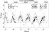 |
Fig. 1 Visual lightcurve of R Scl based on the AAVSO and AFOEV databases. The solid line represents a sine fit to the ten most recent cycles. The dashed vertical lines denote the mean epochs of our 2012 AMBER and 2014 and 2015 PIONIER observations. |
Log of our AMBER observations.
The source R Scl is classified as a carbon-rich SR pulsating AGB star with a period of 370 days (Samus et al. 2009). Maercker et al. (2016) estimated a present-day mass-loss rate of up to 10-6M⊙/yr and a present-day outflow velocity of about 10 km s-1.
The distance to R Scl based on the empirical period-luminosity (P-L) relationships by Knapp et al. (2003) results in 370 pc for SR variables and 340 pc for Mira variables. The P-L relationships for Miras by Groenewegen & Whitelock (1996) and Whitelock et al. (2008) give similar distances of 360 pc and 370 pc, respectively. Sacuto et al. (2011) derived a distance of 350 ± 50 pc by fitting the SED to hydrostatic atmosphere models. The original Hipparcos parallax was uncertain with 2.11 ± 1.52 mas, corresponding to a distance of 474
 pc. The revised Hipparcos parallax (van Leeuwen 2007) of 3.76 ± 0.75 mas corresponds to a distance of 266
 pc. Both Hipparcos parallaxes might be biased because R Scl has a large angular diameter and exhibits surface features. Maercker et al. (2012) and Vlemmings et al. (2013) used a distance of 290 pc in the tradition of Olofsson et al. (2010) and Schöier et al. (2005). Maercker et al. (2016) corrected the distance to the P-L distance of 370 pc. In total, this shows that the distance to R Scl is uncertain. In the following we use the P-L distance
  pc.
pc.
Figure 1 shows the recent visual lightcurve of R Scl based on data obtained from the AAVSO (American Association of Variable Star Observers) and AFOEV (Association Française des Observateurs d’Étoiles Variables) databases. The solid line represents a fit of a sine curve to the ten most recent cycles, and results in a period of 376 days and a Julian date of last maximum of 2 457 372. We indicated in Fig. 1 the mean epochs of our observations, that is, AMBER at a mean JD 2 456 237 and PIONIER at mean JDs 2 456 901 and 2 457 357, corresponding to a maximum phase of 0.98 for our AMBER observations and pre-maximum & maximum phases of 0.75 & 0.96 for our PIONIER observations. The visual lightcurve shows an observed amplitude of about 1.5–2 mag and a regular sinusoidal pulsation. This lightcurve may be more typical for a Mira variable than for a SR variable. In fact, carbon-rich stars generally have a lower visual amplitude than oxygen-rich stars of the same bolometric amplitude, because molecules in the carbon-rich case have a lower temperature sensitivity and lower opacity in the visual compared to oxygen-rich stars. As a result, carbon stars are often classified as SR variables while oxygen-rich stars of the same bolometric lightcurve are classified as Miras (e.g., Kerschbaum & Hron 1992). We placed R Scl on the diagram of the period-luminosity (P-L) sequences by Wood (2015, Fig. 10). This diagram is for the Large Magellanic Cloud (LMC), but Whitelock et al. (2008) did not find significantly different P-L relations for different metallicities. We corrected the apparent J and K magnitudes from the 2 MASS catalog (Cutri et al. 2003) to the distance of the LMC, and obtained a WJK value (cf. Wood 2015) of 9.1 ± 0.4. Together with the pulsation period, R Scl is located on the sequence that corresponds to fundamental mode pulsation. Here, the long pulsation period of 376 days excludes overtone modes, which have significantly lower pulsation periods below about 250 days. Fundamental mode pulsation is again more typical for a Mira variable than for a SR variable, although Wood et al. (1999) noted that some SRs pulsate in fundamental mode.
We integrated available spectro-photometry. We used B and V magnitudes from the SIMBAD (Set of Identifications, Measurements, and Bibliography for Astronomical Data) database (Wenger et al. 2000), the mean J, H, K, L magnitudes from Whitelock et al. (2006), the M magnitude from Le Bertre (1992), and the IRAS 12 μm, 25 μm, 60 μm, 100 μm fluxes from Beichmann (1985), adopting AV = 0.07 from Whitelock et al. (2008) and using the reddening law from Schlegel et al. (1998). We obtained a bolometric flux of fbol = 1.2810-9 W/m2, with an assumed error of 5%.
2.2. AMBER observations and data reduction
We obtained service mode observations of R Scl with the AMBER instrument (Petrov et al. 2007) in the K-band 2.3 μm medium resolution mode employing external FINITO fringe tracking between October and December 2012. Table 1 shows the details of our AMBER observations, including the dates, the Julian day, the baseline configurations with the projected baseline lengths and angles, and the interferometric calibrators used for each observation. Observations of R Scl were interleaved with observations of calibrators in sequences of a calibrator observation taken before the science target observation, the science target observation, and another calibrator observation taken afterward. Calibrators were selected with the ESO Calvin tool, and their angular K-band diameters were adopted from Lafrasse et al. (2010) (HR 109: 3.06 ± 0.22 mas; χ Phe: 2.69 ± 0.03 mas; ιEri: 2.12 ± 0.02 mas). Each of the observations typically consists of five files of 170 scans each, accompanied by a dark and a sky file. It is essential for a good calibration of the interferometric transfer function that the performance of the FINITO fringe tracking is comparable between corresponding calibrator and science target observations. To this purpose, we inspected the FINITO lock ratios and the FINITO phase rms values as reported in the fits headers of each file (cf. Le Bouquin et al. 2009; Mérand et al. 2012). In a few cases, we deselected individual files for which these values deviated significantly from the mean of the calibrator and science files. In a few cases, we had to discard a complete data set because the FINITO phase rms values were systematically very different for all files between science target observation and calibrator observations.
We obtained averaged visibility and closure phase values from the raw data using the latest version, 3.0.9, of the amdlib data reduction package (Tatulli et al. 2007; Chelli et al. 2009). The absolute wavelength calibration and the calibration of the interferometric transfer function were performed using IDL (Interactive Data Language) scripts. For the absolute wavelength calibration, we correlated the AMBER flux spectra with a reference spectrum that included the AMBER transmission curve, the telluric spectrum estimated with ATRAN (Lord 1992), and the expected stellar spectrum using the spectrum of the K giant BS 4371 from Lançon & Wood (2000), which has a similar spectral type as our calibrators. Moreover, we performed a relative flux calibration using the calibrator stars and the BS 4371 spectrum to remove the instrumental and telluric signatures. For calibrating the interferometric transfer function, we used an average transfer function of the calibrator observations obtained before and after that of the science target. The error of the final visibility spectra includes the statistical noise of the raw data and the systematic error of the transfer function calculated as the standard deviation between the two calibrator observations. The resulting calibrated flux and visibility data are shown in Figs. 2–4 and are discussed in Sect. 4.2 together with the atmosphere model results.
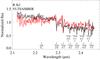 |
Fig. 2 AMBER flux spectrum (black) compared to the prediction by the best-fit dynamic model (red). The blue bars denote the mean errors for the first and second halves of the wavelength range. Instrumental and telluric signatures are calibrated and removed. |
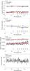 |
Fig. 3 AMBER results (black) compared to the prediction by the best-fit dynamic model (red). The two top panels show the squared visibilities and closure phases versus wavelength for the example of a compact baseline configuration (data set No. 5 in Table 1), followed by an example of an extended configuration (data set No. 9). The blue bars denote the mean errors for the first and second halves of the wavelength range. The three lines correspond to the three baselines of the baseline triplet. |
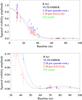 |
Fig. 4 AMBER visibility results as a function of baseline length for the examples of bandpasses in the CO (2-0) line at 2.29 μm and the nearby pseudo-continuum at 2.28 μm. The points with error bars denote the observations. The solid lines denote the synthetic visibility based on the best-fit model atmosphere. The fit was derived from the full data set. The green dotted line shows the result based on the uniform disk (UD) fit. The upper panel shows the full visibility range. The lower panel shows an enlargement of the small visibility values at long baselines. |
2.3. PIONIER observations and data reduction
We obtained interferometry of R Scl with the PIONIER instrument (Le Bouquin et al. 2011) and the four auxiliary telescopes (ATs) of the Very Large Telescope Interferometer (VLTI) between 25 August and 7 September 2014 in designated visitor mode, and on 29 November and 3 December 2015 in service mode. The 2014 observations were taken with the original PICNIC camera (Le Bouquin et al. 2011) and data were dispersed over three spectral channels with central wavelengths 1.59 μm, 1.68 μm, 1.76 μm, and channel widths ~0.09 μm. In 2014, we used all three available baseline configurations, where the ATs were positioned on stations A1/B2/C1/D0 (“small”, ground baseline lengths between 11.3 m and 35.8 m), D0/G1/H0/I1 (“medium”, 40.8–82.4 m), and A1/G1/J3/K0 (“large”, 56.6–140.0 m). The 2015 observations were taken after the upgrade to the RAPID camera (Guieu et al. 2014) and data were dispersed over six spectral channels with central wavelengths 1.53 μm, 1.58 μm, 1.62 μm, 1.68 μm, 1.72 μm, 1.76 μm, and channel widths ~0.05 μm. In 2015, we obtained data on only two of the three baseline configurations, where the ATs were positioned on stations A0/B2/C1/D0 (“small”, 11.3–33.9 m) and A0/G1/J2/J3 (“large”, 58.2–132.4 m), and we obtained only one observation per configuration. Observations of the science targets were interleaved with observations of interferometric calibrators. We selected calibrators from the ESO calibrator selector CalVin, which is based on the catalog by Lafrasse et al. (2010). The calibrators include HD 6629 (spectral type K4 III,  mas, used during 2014-08-25, 2014-08-26, 2014-09-02, 2014-09-06, 2014-09-07), HR 400 (M0 III, 2.45 ± 0.01 mas, 2014-08-25), ξ Scl (K1 III, 1.32 ± 0.02 mas, 2014-08-25), HD 8887 (K0 III, 0.52 ± 0.02 mas, 2014-08-26, 2014-09-02, 2014-09-06, 2014-09-07, 2015-11-28, 2015-12-02), HD 9961 (K2 III, 0.87 ± 0.01 mas, 2014-08-26, 2014-09-02, 2014-09-06, 2014-09-07), HD 8294 (K2 III, 0.70 ± 0.02 mas, 2015-11-28, 2015-12-02), and HR 453 (K0 III, 0.90 ± 0.06 mas, 2015-12-02). Table 2 lists the details of our R Scl PIONIER observations. Figure 5 shows the uv coverage that we obtained in 2014 and 2015.
We reduced and calibrated the data with the pndrs package (Le Bouquin et al. 2011). Each of the listed observations typically consists of five consecutive measurements. Each of these results in six squared visibility amplitudes and four closure phases at three (2014) or six (2015) spectral channels. Not all of these points passed the quality checks that are included in the pndrs package. In total, we secured 4959/198 valid squared visibility amplitudes and 3103/113 valid closure phase values in 2014/2015 on R Scl. The resulting calibrated visibility values are shown in Fig. 6 and are discussed below in Sect. 4.3 together with the atmosphere model results. The quantity and quality of the 2014 data allowed us to reconstruct images of R Scl, which are described in Sect. 4.4. The 2015 data are too few to reconstruct images.
Log of our PIONIER observations.
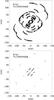 |
Fig. 5 The uv coverage obtained for our PIONIER observations of R Scl in 2014 (top) and 2015 (bottom). |
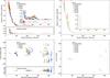 |
Fig. 6 PIONIER results of R Scl as a function of spatial frequency including the squared visibility values (top) and the closure phases (bottom). The left panels show the results obtained in 2014, and the right panels the results obtained in 2015. The vertical bars indicate the symmetric error bars. The central positions of the measured values are omitted for the sake of clarity. The different colors denote the different spectral channels. The dashed lines indicate the best-fit model atmospheres. For the 2014 data, the synthetic values based on the reconstructed images are shown by horizontal bars. Here, the lower small panels provide the residuals between observations and reconstructed images. |
In addition to R Scl, we secured data on the resolved K5/M0 giant υ Cet as a “check star” in order to assess the validity and accuracy of the visibility and closure phase data, in particular for the low fringe contrasts, as well as the consistency between different nights and between the different epochs in 2014 and 2015. The details of these observations are described in Appendix A. These observations confirmed a high accuracy of the low visibility values close to and beyond the first minimum of the visibility function and of the closure phase data. These data allowed us to confirm the strength of the model-predicted limb-darkening effect with high significance. However, the high visibility data at short baselines lay systematically above the model prediction, which is a known effect of PIONIER calibrations and most likely caused by different magnitudes or airmass between science target and calibrators (see Appendix A for more details). In the following, we took this known effect into account for the modeling and imaging processes of R Scl by excluding the short baseline visibility data (baselines shorter than B = 11.5 m), and by accepting that high synthetic visibility values based on the best-fit model prediction or the reconstructed image may lie below the measured values.
3. Atmosphere modeling
We employed the atmosphere model grid for carbon-rich AGB stars constructed by Mattsson et al. (2010) and Eriksson et al. (2014). In particular, we used the data by Eriksson et al. (2014), which correspond to a sub-sample of the Mattsson et al. (2010) grid in terms of stellar parameters, focusing on typical values of solar-metallicity carbon-rich AGB stars. The models assume spherical symmetry and cover dynamic models with effective temperatures between 2600 K to 3200 K, luminosities log L/L⊙ between 3.55 and 4.00, masses between 0.75 M⊙ and 2.0 M⊙, and C/O abundance ratios of 1.35, 1.69, and 2.38. The corresponding pulsation periods lie between 221 days and 525 days. The effects of stellar pulsation are simulated by a variable inner boundary (so-called piston models), characterized by velocity amplitudes Δup of 2 km s-1, 4 km s-1, and 6 km s-1. Finally, a parameter fL describes whether the original luminosity amplitude (as described in Höfner et al. 2003) was used, or twice the luminosity amplitude of the Mattsson et al. (2010) grid, following Nowotny et al. (2010), to better describe observed photometric variations. We note that the stellar parameters mentioned above are those of the hydrostatic starting model. Models were calculated over different cycles. A typical model run for a given set of stellar and pulsation parameters covers several hundred pulsation phases. Of the total of 540 models, some of the models turn out to produce a wind (229), and some do not produce a wind (311). Eriksson et al. (2014) performed detailed radiative transfer calculations to obtain low resolution spectra in the wavelength range 0.35–25 μm and a number of filter magnitudes. For this calculation, they used the opacity generation code COMA (Aringer et al. 2009) to compute continuous atomic, molecular, and amorphous carbon (amC) dust opacities for all atmospheric layers and each wavelength point, assuming local thermodynamic equilibrium (LTE) and assuming the small particle limit for the dust opacities.
Parameters of the considered dynamic models.
Diameter fit results.
From this model grid, we pre-selected models that are broadly consistent with the known parameters of R Scl, the available broad-band photometry (cf. Sect. 2.1), and the available Infrared Space Observatory (ISO) spectra from the Short Wavelength Spectrometer (SWS) (Sloan et al. 2003). The parameters of the considered models are listed in Table 3. We employed three models, and for two of them we selected snapshots at two or three different cycles. Every entry in Table 3 contains 40–60 snapshots at continuous phases. In addition to the stellar parameters described above, Table 3 also lists the corresponding surface gravity, the average mass-loss rate, outflow velocity, and period. The first two of the considered models in Table 3 correspond to effective temperatures of 2600 K with masses 0.75 and 1.0 M⊙. They have mass-loss rates of 3.9 × 10⁻⁷ M⊙/yr and 7.4 × 10⁻⁷ M⊙/yr, respectively, and periods of 294 d. The third model corresponds to an effective temperature of 2800 K, a mass of 1.0 M⊙ and a period of 390 d, and does not produce a mass loss. Other models of the grid with a higher mass or a higher effective temperature lead to luminosities or periods that are not consistent with the observed values for R Scl. However, we cannot fully exclude that another model at certain phases may also explain the data.
Using COMA, we tabulated for every snapshot intensity profiles between 1.4 μm and 2.5 μm at intervals of 0.0001 μm at typically 200–300 radial points between the center and the outer boundary, which depends on the extension of the particular model. The wavelength intervals are chosen such that we can average about ten wavelengths per AMBER spectral channel in its medium spectral resolution mode. We computed synthetic squared visibility amplitudes using the Hankel transform and averaging over the bandpass of every AMBER or PIONIER spectral channel, as described in detail by, for example, Wittkowski et al. (2004). Our primary fit parameter is the angular diameter that corresponds to the arbitrary outermost model layer where the tabulated intensity profiles stop. We use the model structure to relate this arbitrary outermost model layer to the model layer where the Rosseland optical depth is 2/3, and provide a best-fit Rosseland angular diameter ΘRoss corresponding to the Rosseland radius R(τRoss = 2/3). We also integrated the intensities over the stellar disk to calculate the synthetic flux at the AMBER and PIONIER spectral channels.
4. Results
4.1. Diameter fit results
As a first step, we calculated best-fit uniform-disk (UD) diameters for our AMBER data and the two epochs of PIONIER data, and obtained values of 10.5 mas, 10.7 mas, and 11.4 mas, with reduced  values of 2.0, 191, and 106, respectively. We estimate the errors to be about 0.5 mas. These values are consistent with the previous estimates of 10.1 mas by Cruzalèbes et al. (2013) based on previous AMBER data and of 10.2 mas by Sacuto et al. (2011) based on MIDI data. The values of the PIONIER fits are high because of the known systematic calibration problems at high visibilities as discussed in Sect. 2.3 and Appendix A.
Then we compared our data to the dynamic atmosphere and wind models as introduced in Sect. 3. We used a visibility model that takes into account a possible over-resolved component due to large-scale circumstellar dust emission of the form:  where A is the flux fraction of the synthetic stellar contribution, depending on the chosen model from Table 3 and ΘRoss, and (1−A) the flux fraction of an over-resolved dust component.
We added to Table 3 the reduced values of the best-fit snapshot of each model as compared to our AMBER data and our two epochs of PIONIER data. Table 4 lists the details of the best-fit snapshots, including the best-fit values of ΘRoss and A, as well as the phase, luminosity, and derived effective temperature of the best-fit snapshot. All dynamic models provide a better fit to both the AMBER and PIONIER data than the simple UD fit.
The best-fit model overall is model 3 from Table 3 with Teff = 2800 K, L = 7000 L⊙, M = 1 M⊙, that – however – does not produce a wind. The maximum outer boundary for this model is situated a bit above two stellar radii, and the condensation degree for carbon is only a few 10-4. The weighted mean of the best-fit ΘRoss values of the three epochs is 8.9 ± 0.3 mas, and the flux fraction of an over-resolved dust component is 0.05 ± 0.02 for AMBER in the K-band, and 0.02 ± 0.03 for PIONIER in the H-band. Together with the bolometric flux and the distance estimates from Sect. 2.1, this value of ΘRoss corresponds to Teff of 2640 ± 80 K, log L/L⊙ of 3.74 ± 0.18, and RRoss of 355 ± 55 R⊙. These values are consistent with the theoretical values of the best-fit snapshots, except for Teff, which is lower. The period of model 3 is closer to the period of R Scl than that of models 1 and 2. We note that model 3 is the same model that was identified by Sacuto et al. (2011) to best fit their MIDI data of R Scl.
Model 1 provides the next-best values. It has values Teff = 2600 K, L = 5000 L⊙, M = 0.75 M⊙, and produces a mass-loss rate of 3.9 × 10⁻⁷ M⊙/yr with an outflow velocity of 2.3 km s-1. However, the best-fit ΘRoss values based on this model lie between 5.6 mas and 6.1 mas, which is neither consistent with the UD fit nor with the previous measurements by Sacuto et al. (2011) and Cruzalèbes et al. (2013), nor with our imaging result shown below. This angular diameter would correspond to Teff as high as 3200 ± 120 K and RRoss as low as 230 ± 40, R⊙, which are also not consistent with independent estimates. A closer inspection of the synthetic intensity profiles of this model showed that the Rosseland angular diameter is too small, but the CSE of this model is more extended, so that overall the 10% and 30% intensity diameters correspond to those of the best-fit snapshot of model 3. In other words, this model provides formally a similarly good fit to the data, but with a Rosseland radius that is too small compared to independent estimates. This is compensated for by a CSE that is too extended compared to our observations. As a result, we discarded this model. In general, the considered models that produce mass-loss (models 1 and 2) appear to have a CSE that is too extended compared to our observations. This may be related to the fact that it is difficult to produce carbon-rich wind models corresponding to the low end of the observed range of mass loss rates (see, e.g., Mattsson et al. 2010; Eriksson et al. 2014, for a discussion of this problem).
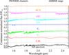 |
Fig. 7 Synthetic continuum-normalized spectra using COMA (Aringer et al. 2009) for the most important molecular species and for the full spectrum. The example spectra of this figure are based on the best-fit model snapshot to our first PIONIER epoch. The resolution of the spectra is 1500, except for C3 and C2H2, which are treated in opacity sampling. Also indicated are the three spectral channels of our PIONIER observations, as well as the range of the AMBER MR 2.3 μm mode. |
Spectra of carbon AGB stars do not show any genuine continuum within the near-IR observing bands, most importantly due to molecular contributions by CO, CN, C2, C2H2, HCN, and C3 (cf., e.g., Gautschy-Loidl et al. 2004; Paladini et al. 2009). All spectral channels of our PIONIER and AMBER observations are thus affected by atomic and molecular features. As an illustration, Fig. 7 shows an example of a synthetic continuum-normalized spectrum, together with the contributions by the individual molecular opacities listed above. This example is based on the best-fit model to our first PIONIER epoch. We used COMA (Aringer et al. 2009) to calculate the spectra, using all available atomic and molecular opacities for the full spectrum, and selecting one molecular opacity at a time for the individual molecular contributions. We show the combined wavelength range of our PIONIER and AMBER observations, covering 1.5–2.5 μm at the resolution of the AMBER medium spectral resolution mode of 1500. The molecules C3 and C2H2 are treated in the opacity sampling method. We indicate the three spectral channels of our PIONIER observations, as well as the range of the used AMBER MR 2.3 μm mode.
4.2. AMBER visibility results and model comparison
Figure 2 shows the observed AMBER flux spectrum of R Scl derived from an average of all AMBER data, together with the prediction by the best-fit dynamic model to the AMBER data. Observed and modeled flux spectra are generally consistent. The spectrum shows an overall flat distribution between 2.12 μm and 2.29 μm with a number of features due to atomic and molecular lines. The most prominent feature within this wavelength range is an absorption line near 2.228 μm. We identified this feature to be mostly a CN band with some contribution from C2, using COMA runs with various variations of atomic and molecular abundances. This feature is relatively weak in the observed flux spectrum but more prominent in the visibility spectra, indicating that it forms at extended layers above the pseudo-continuum. Observed and modeled flux spectra between 2.29 μm and 2.46 μm clearly exhibit the 12CO (2–0, 3–1, 4–2, 5–3, 6–4) and 13CO (2–0, 3–1, 4–2, 5–3) bandheads and show a generally lower flux level due to CO absorption. “Emission”-like features next to CO bandheads are residuals of the telluric correction.
Figure 3 shows the squared visibility amplitudes and closure phases as a function of wavelength for two examples, data set No. 5 from Table 1 obtained with a compact baseline configuration and data set No. 9 obtained with an extended baseline configuration. The synthetic values based on the best-fit dynamic model are shown as well. The shown errors are dominated by the systematic uncertainty of the global height of the interferometric transfer function. The wavelength-differential errors are small compared to the systematic error, as evidenced by the small pixel-to-pixel variations. The observed visibility spectra are generally flat as a function of wavelength and consistent with the dynamic model. The observed squared visibility values show drops at the positions of the 12CO bandheads between 2.3 μm and 2.5 μm as well as at the position of the CN band near 2.228 μm. This is best visible at squared visibility levels of 0.1–0.2 and indicates that these lines are formed at extended layers above the pseudo-continuum. This behavior is comparable to oxygen-rich SR AGB stars (e.g., Martí-Vidal et al. 2011). The 13CO bandheads are less prominent in the visibility spectra than in the flux spectrum, which may indicate that 13CO is less extended than 12CO. Wavelength-differential closure phase features at the positions of the CO bandheads indicate photocenter displacements between the CO-forming regions and the nearby pseudo-continuum.
Figure 4 shows the AMBER visibility results of all data sets as a function of baseline length for the examples of bandpasses in the CO (2–0) line at 2.29 μm and the nearby pseudo-continuum at 2.28 μm together with the model prediction in these bandpasses. It illustrates that R Scl is more extended in the CO (2–0) bandpass compared to the nearby pseudo continuum, and that this behavior is consistent with the model prediction. The difference between the two bandpasses might be slightly larger in the observations than in the model prediction. The UD fit lies in between the model prediction at these bandpasses and – as a wavelength independent model – cannot reproduce the visibility differences.
4.3. PIONIER visibility results and model comparison
Figure 6 shows all our PIONIER squared visibility (top) and closure phase (bottom) data as a function of spatial frequency. PIONIER data obtained in 2014 are shown in the left panels, and those obtained in 2015 in the right panels. We indicate the synthetic visibility based on the best-fit snapshots by dashed lines. For the 2014 data, we also show the visibility values based on the reconstructed image as discussed below in Sect. 4.4, as well as their residuals relative to the measured values.
The observed visibility values show a characteristic curve of a resolved stellar disk. The squared visibility amplitudes in the first lobe up to the first minimum at a spatial frequency of ~130 cycles/arcsec are consistent with the synthetic curve based on a spherical model, while the squared visibility amplitudes at higher spatial frequencies cannot be well described by the spherical model. Consistently, the closure phase values are consistent with zero up to maximum spatial frequencies of about 90 cycles/arcsec, shortly before the minimum of the squared visibility, then start to deviate from zero values between about 90–110 cycles, and show a very complex behavior at higher observed maximum spatial frequencies between 180 cycles/arcsec and 440 cycles/arcsec. This behavior of the squared visibility amplitudes and closure phases indicate a broadly circular resolved stellar disk with a complex substructure.
The squared visibility amplitudes at short spatial frequencies up to about 50/cycles lie systematically above the model predictions. We have seen the same behavior for the well-known check star υ Cet (Appendix A) and attribute it to known systematic calibration effects owing to different magnitudes or airmass between the science target and the calibrator (cf. Sect. 2.3).
The squared visibility amplitudes in the first lobe indicate that the source is slightly more extended at the 1.59 μm spectral channel compared to the 1.68 μm and 1.76 μm spectral channels in the 2014 data, as well as at the bluer spectral channels at 1.53 μm and 1.58 μm compared to the redder spectral channels at 1.68 μm to 1.76 μm in the 2015 data. This result is also predicted by the best-fit model snapshots. A larger extension at central wavelengths of 1.53–1.59 μm might be related to the “1.53 μm feature”, which was discussed by Gautschy-Loidl et al. (2004) and attributed to C2H2 and HCN (cf. also Fig. 7).
The closure phases starting from maximum spatial frequencies of about 100 cycles/arcsec and more clearly around 200 cycles/arcsec show closure phase values decreasingly different from zero across the three 2014 spectral channels from 1.59 μm to 1.76 μm, indicating differences in the substructure of the stellar disk at the three spectral channels.
4.4. PIONIER imaging
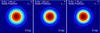 |
Fig. 8 Image representations of the intensity profiles of the best-fit dynamic model snapshot. The three images represent the three PIONIER spectral channels with central wavelengths 1.59 μm (left), 1.68 μm (middle), and 1.76 μm (right). All images are based on the same Rosseland angular diameter. The images are convolved with a theoretical point spread function (PSF) using a Gaussian with FWHMλcentral/Bmax. The Rosseland angular diameter is indicated by the dashed black circle. Contours are drawn at levels of 0.9, 0.7, 0.5, 0.3, 0.1. |
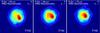 |
Fig. 9 Image reconstructions of R Scl based on our 2014 PIONIER data and the IRBis image reconstruction package (Hofmann et al. 2014). The three images represent the three PIONIER spectral channels with central wavelengths 1.59 μm (left), 1.68 μm (middle), and 1.76 μm (right). The images are convolved with a theoretical point spread function (PSF) using a Gaussian with FWHMλcentral/Bmax. Our estimate of the Rosseland angular diameter is indicated by the dashed black circle. Contours are drawn at levels of 0.9, 0.7, 0.5, 0.3, 0.1. |
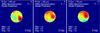 |
Fig. 10 Image reconstructions of R Scl from Fig. 9 divided by the model images from Fig. 8 in order to remove the global center-to-limb intensity variation and to highlight the surface structure on top of this variation. We use a cut-off radius at a model intensity level of 50%, located slightly within the Rosseland radius, which is indicated by the black dashed circle. We calculated the maximum, minimum, and mean intensities inside the cut-off radius to estimate the contrast of the observed structure and printed them on the image. These values are normalized to an average intensity of unity for each spectral channel separately. Contours are drawn at levels of 0.9, 0.7, 0.5. |
We used the IRBis image reconstruction package by Hofmann et al. (2014) to reconstruct images based on our 2014 PIONIER data at each of the three spectral channels. This image reconstruction package currently offers six different regularization functions. It offers the use of a start image. Most of the regularization functions can be used with a prior image or with a flat prior. For details on the image reconstruction algorithms, we refer to the original article by Hofmann et al. (2014). We chose to use the model images based on the best-fit model snapshot as start images. We used a flat prior, and smoothness as regularization function (regularization function 3 of Hofmann et al. 2014).
In order to verify the imaging process, we studied the effects of using the different available regularization methods of IRBis. We studied as well the effects of using other image reconstruction packages, namely MiRA by Thiébaut (2008) and BSMEM by Buscher (1994). These studies also included the use of different start images and different prior images. The results of these imaging studies are detailed in Appendix B. These studies show that the reconstructed images are very stable with respect to using different image reconstruction packages and algorithms, different regularization functions, different start images, and different prior images.
We used start images based on the best-fit model snapshots for the imaging with IRBis. Figure 8 shows the model images based on the intensity profiles of the best-fit dynamic model snapshots. Indicated are the positions of the estimated Rosseland radius as well as contours at levels of 0.9, 0.7, 0.5, 0.3, and 0.1. The images show a center-to-limb intensity variation with a steep decrease of the intensity profiles between intensity levels of 0.5 and 0.3, which is located near the estimated Rosseland radius of 8.8 mas. Beyond the Rosseland radius, the images show a shallow extension reaching a 10% intensity level at an angular diameter of about 15.2 mas (~1.7 ΘRoss) for the spectral channel with central wavelength 1.59 μm and about 13.6 mas (~1.5 ΘRoss) for spectral channels with central wavelengths of 1.68 μm and 1.76 μm. Likewise, the steep decrease near intensity levels between 50% and 30% is slightly shallower for the spectral channel at 1.59 μm compared to the two redder spectral channels. This difference between the 1.59 μm channel compared to the 1.68 μm and 1.76 μm channels was confirmed by our measured visibility data in Sect. 4.3 and may be an effect of extended layers of C2H2 and HCN (“1.53 μm feature”, Gautschy-Loidl et al. 2004). These model images are used as start images, but not as prior images, for the following image reconstruction process. However, our image reconstructions using the MiRA package (Thiébaut 2008), shown in Appendix B, used a simple UD fit as a start image, and gave virtually identical results, showing that the choice of the start image was not critical.
Figure 9 shows our reconstructed images for the three spectral channels. These images are convolved with a theoretical point spread function (PSF) using a Gaussian with FWHM λcentral/Bmax. We have added the squared visibility amplitudes and closure phases based on the reconstructed images to Fig. 6, which shows the measured values. The residuals between imaging values and measured values are shown as well. The synthetic visibility values based on the reconstructions are in very good agreement with the measured values, except for high squared visibility amplitudes at small spatial frequencies. The latter was expected, due to known systematic calibration effects (Sect. 4.3 and Appendix A). It is thus re-assuring that the imaging processes kept these differences between reconstructed images and measured visibility values, and did not correct for these systematic calibration effects by artificial features in the reconstructions.
As expected from the visibility results discussed in Sect. 4.3, the reconstructed images show a broadly circular stellar disk with a very complex substructure. The global center-to-limb intensity variation is broadly consistent with the model images discussed above: our estimate of the Rosseland angular diameter is on average located between the 50% and 30% intensity levels, as in the model images. The extension of the 10% intensity level is comparable to that of the model images as well. Furthermore, the contours at 10% and 30% of the maximum intensity are roughly circular, while the higher intensity levels above about 50%, located inside the Rosseland angular diameter, that is, inside the stellar disk, show a very complex structure. Most strikingly, the images show one dominant bright spot located at the western part of the stellar disk, adjacent to a bright region toward the north-east of the bright spot.
The complex structure that we observed within the stellar disk is superimposed on the global center-to-limb intensity variation. In order to remove the signature of the global center-to-limb intensity variation and to study the structure on top of this variation, we divided the reconstructed images shown in Fig. 9 by the model images shown in Fig. 8. Figure 10 shows the divided images. We used a cut-off radius at a model intensity level of 50%, located slightly inside the Rosseland radius, outside of which we set the divided images to zero. We calculated the maximum, minimum, and mean intensities inside the cut-off radius to estimate the contrast of the observed structure. The peak intensity of the dominant western spot lies 58%, 42%, and 46% above the average intensity (including the spot itself) at the three spectral channels with central wavelengths of 1.59 μm, 1.68 μm, and 1.76 μm, respectively. The total contrast between the minimum and maximum intensities within this part of the stellar disk are 1:2.3, 1:2.1, and 1:2.8, respectively. We estimate the errors of the intensities to be about 5–10%. These divided images show more clearly than the original ones that the dominant spot is slightly shifted from south-west to west to north-west across the spectral channels at 1.59 μm, 1.68 μm, and 1.76 μm. This may be related to the differences in the closure phases across these spectral channels at ~200 cycles/arcsec (cf. Sect. 4.3, Fig. 6). However, we cannot currently exclude an uncertainty of the position of the dominant spot of this order in the imaging process.
4.5. Fundamental parameters of R Scl
Fundamental properties of R Scl used in this work.
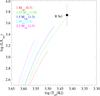 |
Fig. 11 Position of R Scl in the HR diagram together with evolutionary tracks by Lagarde et al. (2012). The tracks are those without rotation and reach up to the start of the TP-AGB. Masses are ZAMS masses; values in parenthesis are masses at the start of the TP-AGB, that is, at the end of the shown tracks. |
Table 5 summarizes the fundamental parameters of R Scl that we used in this work, including our adopted values for the bolometric flux and distance, the measured Rosseland angular diameter, and the derived effective temperature and luminosity. We note that the distance to R Scl is quite uncertain, as discussed in Sect. 2.1, which is reflected in its large adopted error. Figure 11 shows the position of R Scl in the Hertzsprung-Russell (HR) diagram based on the effective temperature and luminosity. This figure includes stellar evolutionary tracks by Lagarde et al. (2012) for zero age main sequence (ZAMS; initial) masses between 1 and 2.5 M⊙. These tracks reach up to the start of the thermally pulsing (TP) AGB, at which point the mass range is 0.7 to 2.5 M⊙. The position of R Scl is consistent with an evolutionary phase shortly beyond the start of the TP-AGB and with an initial mass interval between 1 and 2 M⊙. We also compared the position of R Scl to the tracks of the TP-AGB by Marigo et al. (2013) as shown by Klotz et al. (2013). Here, R Scl is also consistent with masses at the start of the TP-AGB between about 1 and 2 M⊙, that is, not significantly below 1 M⊙ and not significantly above 2 M⊙. These are evolutionary tracks for single stars, while a binary companion has been detected for R Scl. However, based on the estimates for the binary companion mass and separation (Maercker et al. 2016), it is unlikely that the companion has affected the evolution of R Scl to the AGB. As a result, we estimate the initial mass of R Scl to be 1.5 ± 0.5 M⊙ and the current mass to be 1.3 ± 0.6 M⊙. Together with our estimate of the radius, these values correspond to a surface gravity log g of –0.6 ± 0.4.
The mass of R Scl can also be estimated by the pulsation properties. We used the formula 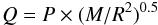 from Wood (1990), where Q is the pulsation constant, and M and R are the mass and radius in solar units. We estimated a Q value of 0.093 ± 0.005 for the given ranges of masses and pulsation periods based on Fox & Wood (1982) and assuming fundamental pulsation mode (cf. Sect. 2.1). We obtained a mass based on these pulsation properties and the measured radius of 2.7 M⊙ and an uncertainty range between 1.5 and 4.7 M⊙. Within the errors, this mass estimate is consistent with the estimate above based on the position in the HR-diagram and the evolutionary models between 1.5 and 1.9 M⊙. The mass based on the evolutionary tracks is mostly constrained by the effective temperature, whose estimate is independent of the distance, while the pulsation mass depends on the radius, and thus the distance. A lower distance within the quoted errors would thus lead to a better agreement between these two mass estimates. For example, a distance of 300 pc at the lower end of our estimate would lead to a pulsation mass of 1.4 M⊙.
We chose to use the mass estimate based on the evolutionary tracks as our final mass estimate in Table 5, because this mass estimate is less affected by the large uncertainty of the distance to R Scl. However, the given errors do not include errors inherent in choosing the particular set of evolutionary tracks.
5. Discussion of the observed structure within the stellar disk
Freytag & Höfner (2008) presented three-dimensional (3D) radiative hydrodynamical simulations of the atmosphere and wind of an AGB star. They concluded that large-scale convective flows, and the resulting atmospheric shock waves, induce certain non-radial structures in the region of the innermost dust shell. We interpret our observed structure on the surface of R Scl within this context.
In this scheme, our observed structure on the stellar disk of R Scl is mostly due to dust absorption and lack thereof, depending on how dense and close to the star the dust is with respect to the line of sight. In this view, the dominant bright spot would be caused by a region where the stellar surface is less obscured by dust clouds. For example, Fig. 2 of Freytag & Höfner (2008) shows arcs in two-dimensional (2D) slices of newly formed dust that are spread over typical angles of about 90 deg. These arcs of newly formed dust, if seen face-on on top of the photosphere, would be qualitatively consistent with our observed structure in terms of the angular scales. Dust clumps of amorphous carbon (amC) located near the condensation radius can efficiently block the light at near-infrared wavelengths so that this scheme is also qualitatively consistent with our observations in terms of the high observed intensity contrasts. These scales are representative of the density structure at 2–3 stellar radii, where the more small-scale photospheric shocks corresponding to the convective flows have merged, forming these partial near-spherical shells that cover a wide angle, and where new dust forms. Molecules at these radii should reflect these density structures corresponding to the large-scale shocks as well, but may not lead to the observed high contrasts. We expect the actual convective surface patterns at photospheric layers to be obscured in the near-IR by molecular (cf. Fig. 7) and dusty layers located above the photosphere.
Freytag & Höfner (2008) already noted that such dust structures, which developed in their 3D simulations, should be detectable by high spatial resolution techniques. Indeed, Ohnaka et al. (2016) and Khouri et al. (2016) observed clumpy dust clouds around the oxygen-rich AGB stars W Hya and R Dor using VLT/SPHERE, which are seen in scattered visual light around the stellar photosphere. The sizes of these clumps are qualitatively consistent with those predicted by Freytag & Höfner (2008). In particular, the dust clouds shown by Ohnaka et al. (2016, Fig. 8) are interpreted as atmospheric structures with a half opening angle of 45 deg, that is, 90 deg total, and a density enhancement of four compared to the surrounding medium. Equivalently, we interpret our detected structure of the carbon-rich AGB R Scl as being caused by absorption by amC dust in front of the star instead of by scattering next to the star. Moreover, amC dust has a higher absorption coefficient than oxygen-rich dust, and can thus lead to higher intensity contrasts.
The 3D simulations do not necessarily predict one single region that vastly dominates our view onto the stellar disk as observed in our reconstructed images. The simulations show a variability on a timescale of a few months, with features that may vary from one to a few months. In our picture, we would have observed the star when the view was dominated by one feature. Unfortunately, our second epoch observations did not result in images so we could not probe the time variability of the observed structure. Yet, such time-linked observations are of great importance to further constrain and verify the model predictions. With our single epoch of reconstructed images we cannot exclude whether the dominant bright spot might be more stable than predicted by simulations based on convection, or whether there may be additional physical mechanisms such as magnetic effects that enhance or stabilize the structure.
Compared to other carbon AGB stars, our observation of a strong clumpiness of the CSE of R Scl is consistent with earlier detections of asymmetries or inhomogeneities toward carbon AGB stars (Paladini et al. 2012; van Belle et al. 2013). Compared to the extreme clumpiness of the circumstellar environment of IRC +10 216 (Weigelt et al. 1998, 2002; Osterbart et al. 2000; Kim et al. 2015; Stewart et al. 2016), our observations of R Scl differ in two important aspects: (1) In our reconstructed near-infrared H-band images of R Scl, the stellar disk is still visible and only partially obscured by an optically thin CSE, while the stellar disk of IRC +10 216 is completely obscured at near-infrared wavelengths to the point that there has been a decade-long debate on the position of the star with respect to the clumps of the circumstellar environment; (2) In our interpretation of R Scl, the near-infrared observations show newly formed dust clumps near the photosphere at 2–3 stellar radii, while the near-infrared observations of the dust clumps of IRC +10 216 cover a volume of roughly 10–20 stellar radii. In both interpretations, the bright spots are interpreted as cavities in a dense circumstellar shell.
The binary companion of R Scl at an estimated separation of 60 AU (Maercker et al. 2012, 2016) is not expected to have a direct influence on the surface and close circumstellar environment of the primary AGB star. Only if the observed structure and the dominant bright spot turn out to be more stable than predicted by the convection simulations on timescales of several years, localized mass loss together with the binary motion may induce shaping close to the surface of R Scl. Again, time series of observations are needed to probe the timescales of the detected structure in order to constrain the convection simulations and to study whether further physical mechanisms may have to be taken into account.
6. Summary and conclusions
We observed the atmosphere and the close CSE of the carbon-rich AGB star R Scl employing near-infrared interferometric techniques. We obtained near-infrared K-band interferometry with a spectral resolution of 1500 using the AMBER instrument in 2012, at a maximum visual phase of R Scl of 1.0. We also obtained near-infrared H-band interferometry with spectral resolutions of about 20 and 40 in 2014 and 2015 at pre-maximum and maximum phases of R Scl of 0.8 and 1.0. The PIONIER observations obtained in 2014 had a sufficient coverage of the uv-plane so that we were successful in reconstructing images of R Scl at the three spectral channels with central wavelengths of 1.59 μm, 1.68 μm, and 1.76 μm, and bandwidths of about 0.09 μm.
The visibility data in the first lobe indicate a broadly circular resolved stellar disk with a uniform disk (UD) diameter of about 10.9 ± 0.5 mas, which is consistent with previous estimates. The AMBER data indicate more extended layers of CN and 12CO lying above the pseudo-continuum. Lines of 13CO are visible in the flux spectrum but are less prominent in the visibility spectra, possibly indicating that 13CO is less extended. Likewise, the PIONIER data indicate a larger extension at the spectral channel at 1.59 μm compared to the other spectral channel, which is likely caused by the “1.53 μm feature” of inhomogeneous extended layers of C2H2 and HCN. The visibility data in the second lobe and the closure phase data indicate a complex substructure within the resolved stellar disk.
We compared our visibility data to a recent grid of one-dimensional (1D) dynamic atmosphere and wind models for carbon-rich AGB stars. We obtained a best fit to all data for a model with averaged effective temperature 2800 K, luminosity log L/L⊙ 3.85, mass 1 M⊙, and period 390 d, which does not produce a mass loss. The latter is unexpected, as R Scl is surrounded by a large circumstellar environment and estimates of the present day outflow velocity suggest a value of about 10 km s-1. However, we do not know the current mass-loss rate, which may be smaller than 10-6 M⊙/yr. Considered models with mass loss generally show a CSE that is too extended compared to our observations.
Based on the model comparisons, we estimate a Rosseland angular diameter of R Scl of 8.9 ± 0.3 mas. Together with the estimated bolometric flux and distance of R Scl, this value corresponds to a Rosseland radius of 355 ± 55 R⊙, an effective temperature of 2640 ± 80 K, and a luminosity of log L ~ 3.74 ± 0.18. Compared to evolutionary tracks, these parameters are consistent with initial masses of 1.5 ± 0.5 M⊙ and current masses of 1.3 ± 0.7 M⊙.
The reconstructed images of R Scl based on the 2014 PIONIER data show a broadly circular stellar disk with a complex, non-spherical substructure, as expected based on a visual inspection of the visibility data. The global center-to-limb intensity variation (CLV) of the reconstructed images is consistent with that of the best-fit models. Inside the stellar disk, the reconstructed images show a very complex structure. Most strikingly, they exhibit one dominant bright spot located at the western part of the stellar disk, adjacent to a bright region toward the north-east of the bright spot. We corrected the reconstructed images for the overall CLV, and estimated a peak intensity of the dominant western spot between about of 45% and 60% on top of the average CLV-corrected intensity. The total contrast between the minimum and maximum CLV-corrected intensities of the stellar disk are between about 1:2 and 1:3.
We interpreted this complex structure within the stellar disk of R Scl as caused by the effects of large-scale convection cells that lead to almost spherical shock fronts, but which develop certain non-radial structures in the innermost dust shell as predicted by 3D radiative hydrodynamical simulations. Within this interpretation, our observed structure on the stellar disk of R Scl is mostly due to dust absorption and lack thereof, depending on how dense and close to the star the dust is with respect to the line of sight. The dominant bright spot would be caused by a region where the stellar surface is less obscured by dust clouds. The scales and contrasts of the observed structure roughly agree with the model predictions as far as they can be probed by our single epoch of broad-band PIONIER images. Certainly, time-resolved images at higher spectral resolution are needed to confirm and constrain this interpretation.
Acknowledgments
C.P. is supported by the Belgian Fund for Scientific Research F.R.S.- FNRS. We acknowledge with thanks the variable star observations from the AAVSO International Database contributed by observers worldwide and used in this research. This research has made use of the SIMBAD and AFOEV databases, operated at CDS, France.
References
- Aringer, B., Girardi, L., Nowotny, W., Marigo, P., & Lederer, M. T. 2009, A&A, 503, 913 [NASA ADS] [CrossRef] [EDP Sciences] [Google Scholar]
- Arroyo-Torres, B., Wittkowski, M., Marcaide, J. M., & Hauschildt, P. H. 2013, A&A, 554, A76 [NASA ADS] [CrossRef] [EDP Sciences] [Google Scholar]
- Beichmann, C. A. 1985, Infrared Astronomical Satellite (IRAS) catalogs and atlases. Explanatory supplement (Pasadena: Jet Propulsion Laboratory) [Google Scholar]
- Buscher, D. F. 1994, in Very High Angular Resolution Imaging, eds. J. G. Robertson, & W. J. Tango, IAU Symp., 158, 91 [Google Scholar]
- Cernicharo, J., Marcelino, N., Agúndez, M., & Guélin, M. 2015, A&A, 575, A91 [NASA ADS] [CrossRef] [EDP Sciences] [Google Scholar]
- Chelli, A., Utrera, O. H., & Duvert, G. 2009, A&A, 502, 705 [NASA ADS] [CrossRef] [EDP Sciences] [Google Scholar]
- Cruzalèbes, P., Jorissen, A., Rabbia, Y., et al. 2013, MNRAS, 434, 437 [NASA ADS] [CrossRef] [Google Scholar]
- Cutri, R. M., Skrutskie, M. F., van Dyk, S., et al. 2003, VizieR Online Data Catalog: II/246 [Google Scholar]
- Decin, L., Richards, A. M. S., Neufeld, D., et al. 2015, A&A, 574, A5 [NASA ADS] [CrossRef] [EDP Sciences] [Google Scholar]
- Eriksson, K., Nowotny, W., Höfner, S., Aringer, B., & Wachter, A. 2014, A&A, 566, A95 [NASA ADS] [CrossRef] [EDP Sciences] [Google Scholar]
- Fleischer, A. J., Gauger, A., & Sedlmayr, E. 1992, A&A, 266, 321 [NASA ADS] [Google Scholar]
- Fox, M. W., & Wood, P. R. 1982, ApJ, 259, 198 [NASA ADS] [CrossRef] [Google Scholar]
- Freytag, B., & Höfner, S. 2008, A&A, 483, 571 [NASA ADS] [CrossRef] [EDP Sciences] [Google Scholar]
- Gautschy-Loidl, R., Höfner, S., Jørgensen, U. G., & Hron, J. 2004, A&A, 422, 289 [NASA ADS] [CrossRef] [EDP Sciences] [Google Scholar]
- Groenewegen, M. A. T., & Whitelock, P. A. 1996, MNRAS, 281, 1347 [NASA ADS] [CrossRef] [Google Scholar]
- Guieu, S., Feautrier, P., Zins, G., et al. 2014, in Optical and Infrared Interferometry IV, Proc. SPIE, 9146, 91461N [NASA ADS] [CrossRef] [Google Scholar]
- Hofmann, K.-H., Weigelt, G., & Schertl, D. 2014, A&A, 565, A48 [NASA ADS] [CrossRef] [EDP Sciences] [Google Scholar]
- Höfner, S., Gautschy-Loidl, R., Aringer, B., & Jørgensen, U. G. 2003, A&A, 399, 589 [NASA ADS] [CrossRef] [EDP Sciences] [Google Scholar]
- Kerschbaum, F., & Hron, J. 1992, A&A, 263, 97 [NASA ADS] [Google Scholar]
- Khouri, T., Maercker, M., Waters, L. B. F. M., et al. 2016, A&A, 591, A70 [NASA ADS] [CrossRef] [EDP Sciences] [Google Scholar]
- Kim, H., Lee, H.-G., Mauron, N., & Chu, Y.-H. 2015, ApJ, 804, L10 [NASA ADS] [CrossRef] [Google Scholar]
- Klotz, D., Paladini, C., Hron, J., et al. 2013, A&A, 550, A86 [NASA ADS] [CrossRef] [EDP Sciences] [Google Scholar]
- Knapp, G. R., Pourbaix, D., Platais, I., & Jorissen, A. 2003, A&A, 403, 993 [NASA ADS] [CrossRef] [EDP Sciences] [Google Scholar]
- Lafrasse, S., Mella, G., Bonneau, D., et al. 2010, VizieR Online Data Catalog: II/300 [Google Scholar]
- Lagarde, N., Decressin, T., Charbonnel, C., et al. 2012, A&A, 543, A108 [NASA ADS] [CrossRef] [EDP Sciences] [Google Scholar]
- Lançon, A., & Wood, P. R. 2000, A&AS, 146, 217 [NASA ADS] [CrossRef] [EDP Sciences] [Google Scholar]
- Le Bertre, T. 1992, A&AS, 94, 377 [NASA ADS] [Google Scholar]
- Le Bouquin, J.-B., Absil, O., Benisty, M., et al. 2009, A&A, 498, L41 [NASA ADS] [CrossRef] [EDP Sciences] [Google Scholar]
- Le Bouquin, J.-B., Berger, J.-P., Lazareff, B., et al. 2011, A&A, 535, A67 [NASA ADS] [CrossRef] [EDP Sciences] [Google Scholar]
- Lord, S. D. 1992, A new software tool for computing Earth’s atmospheric transmission of near- and far-infrared radiation, Tech. Rep. [Google Scholar]
- Maercker, M., Mohamed, S., Vlemmings, W. H. T., et al. 2012, Nature, 490, 232 [NASA ADS] [CrossRef] [PubMed] [Google Scholar]
- Maercker, M., Vlemmings, W. H. T., Brunner, M., et al. 2016, A&A, 586, A5 [NASA ADS] [CrossRef] [EDP Sciences] [Google Scholar]
- Marigo, P., Bressan, A., Nanni, A., Girardi, L., & Pumo, M. L. 2013, MNRAS, 434, 488 [NASA ADS] [CrossRef] [Google Scholar]
- Martí-Vidal, I., Marcaide, J. M., Quirrenbach, A., et al. 2011, A&A, 529, A115 [NASA ADS] [CrossRef] [EDP Sciences] [Google Scholar]
- Mattsson, L., Wahlin, R., & Höfner, S. 2010, A&A, 509, A14 [NASA ADS] [CrossRef] [EDP Sciences] [Google Scholar]
- Mérand, A., Patru, F., Berger, J.-P., Percheron, I., & Poupar, S. 2012, in Optical and Infrared Interferometry III, Proc. SPIE, 8445, 84451K [Google Scholar]
- Nowotny, W., Höfner, S., & Aringer, B. 2010, A&A, 514, A35 [NASA ADS] [CrossRef] [EDP Sciences] [Google Scholar]
- Ohnaka, K., Weigelt, G., & Hofmann, K.-H. 2016, A&A, 589, A91 [NASA ADS] [CrossRef] [EDP Sciences] [Google Scholar]
- Olofsson, H., Bergman, P., Eriksson, K., & Gustafsson, B. 1996, A&A, 311, 587 [NASA ADS] [Google Scholar]
- Olofsson, H., Maercker, M., Eriksson, K., Gustafsson, B., & Schöier, F. 2010, A&A, 515, A27 [NASA ADS] [CrossRef] [EDP Sciences] [Google Scholar]
- Osterbart, R., Balega, Y. Y., Blöcker, T., Men’shchikov, A. B., & Weigelt, G. 2000, A&A, 357, 169 [NASA ADS] [Google Scholar]
- Paladini, C., Aringer, B., Hron, J., et al. 2009, A&A, 501, 1073 [NASA ADS] [CrossRef] [EDP Sciences] [Google Scholar]
- Paladini, C., Sacuto, S., Klotz, D., et al. 2012, A&A, 544, L5 [NASA ADS] [CrossRef] [EDP Sciences] [Google Scholar]
- Petrov, R. G., Malbet, F., Weigelt, G., et al. 2007, A&A, 464, 1 [NASA ADS] [CrossRef] [EDP Sciences] [Google Scholar]
- Quintana-Lacaci, G., Cernicharo, J., Agúndez, M., et al. 2016, ApJ, 818, 192 [NASA ADS] [CrossRef] [Google Scholar]
- Rau, G., Paladini, C., Hron, J., et al. 2015, A&A, 583, A106 [NASA ADS] [CrossRef] [EDP Sciences] [Google Scholar]
- Rau, G., Hron, J., Paladini, C., et al. 2017, A&A, 600, A92 [NASA ADS] [CrossRef] [EDP Sciences] [Google Scholar]
- Sacuto, S., Aringer, B., Hron, J., et al. 2011, A&A, 525, A42 [NASA ADS] [CrossRef] [EDP Sciences] [Google Scholar]
- Samus, N. N., Durlevich, O. V., et al. 2009, VizieR Online Data Catalog: B/gcv [Google Scholar]
- Schlegel, D. J., Finkbeiner, D. P., & Davis, M. 1998, ApJ, 500, 525 [NASA ADS] [CrossRef] [Google Scholar]
- Schöier, F. L., Lindqvist, M., & Olofsson, H. 2005, A&A, 436, 633 [NASA ADS] [CrossRef] [EDP Sciences] [Google Scholar]
- Sloan, G. C., Kraemer, K. E., Price, S. D., & Shipman, R. F. 2003, ApJS, 147, 379 [NASA ADS] [CrossRef] [Google Scholar]
- Stewart, P. N., Tuthill, P. G., Monnier, J. D., et al. 2016, MNRAS, 455, 3102 [NASA ADS] [CrossRef] [Google Scholar]
- Tatulli, E., Millour, F., Chelli, A., et al. 2007, A&A, 464, 29 [NASA ADS] [CrossRef] [EDP Sciences] [Google Scholar]
- Thiébaut, E. 2008, in Optical and Infrared Interferometry, Proc. SPIE, 7013, 70131I [Google Scholar]
- van Belle, G. T., Paladini, C., Aringer, B., Hron, J., & Ciardi, D. 2013, ApJ, 775, 45 [NASA ADS] [CrossRef] [Google Scholar]
- van Leeuwen, F. 2007, A&A, 474, 653 [NASA ADS] [CrossRef] [EDP Sciences] [Google Scholar]
- Vlemmings, W. H. T., Maercker, M., Lindqvist, M., et al. 2013, A&A, 556, L1 [NASA ADS] [CrossRef] [EDP Sciences] [Google Scholar]
- Wachter, A., Schröder, K.-P., Winters, J. M., Arndt, T. U., & Sedlmayr, E. 2002, A&A, 384, 452 [NASA ADS] [CrossRef] [EDP Sciences] [Google Scholar]
- Weigelt, G., Balega, Y., Bloecker, T., et al. 1998, A&A, 333, L51 [NASA ADS] [Google Scholar]
- Weigelt, G., Balega, Y. Y., Blöcker, T., et al. 2002, A&A, 392, 131 [NASA ADS] [CrossRef] [EDP Sciences] [Google Scholar]
- Wenger, M., Ochsenbein, F., Egret, D., et al. 2000, A&AS, 143, 9 [NASA ADS] [CrossRef] [EDP Sciences] [Google Scholar]
- Whitelock, P. A., Feast, M. W., Marang, F., & Groenewegen, M. A. T. 2006, MNRAS, 369, 751 [NASA ADS] [CrossRef] [EDP Sciences] [Google Scholar]
- Whitelock, P. A., Feast, M. W., & van Leeuwen, F. 2008, MNRAS, 386, 313 [NASA ADS] [CrossRef] [Google Scholar]
- Wittkowski, M., Aufdenberg, J. P., & Kervella, P. 2004, A&A, 413, 711 [NASA ADS] [CrossRef] [EDP Sciences] [Google Scholar]
- Wood, P. R. 1990, in Confrontation Between Stellar Pulsation and Evolution, eds. C. Cacciari, & G. Clementini, ASP Conf. Ser., 11, 355 [Google Scholar]
- Wood, P. R. 2015, MNRAS, 448, 3829 [NASA ADS] [CrossRef] [Google Scholar]
- Wood, P. R., Alcock, C., Allsman, R. A., et al. 1999, in Asymptotic Giant Branch Stars, eds. T. Le Bertre, A. Lebre, & C. Waelkens, IAU Symp., 191, 151 [Google Scholar]
Appendix A: PIONIER observations of the resolved K5/M0 III star υ Cet
In addition to the PIONIER observations of R Scl, we secured a few data points on the nearby resolved K5/M0 giant υ Cet as a “check star”, using every baseline configuration that was used for R Scl. The aim of these observations was to test the validity of the visibility and closure phase data based on a star that can be well described a priori. To describe the star, we used the grid of PHOENIX model atmospheres as introduced by Arroyo-Torres et al. (2013) and chose an effective temperature of 4000 K and a surface gravity of log g = 1 based on the spectral type. We can expect that a regular K or early M giant can be well described by this model atmosphere. We took data on υ Cet on 2014-08-25 (1 observation), 2014-09-02 (2 obs.), 2014-09-06 (1 obs.), 2014-09-07 (1 obs.), 2015-11-28 (1 obs.), and 2015-12-02 (1 obs.). We tested the consistency of measured and modeled visibility values and closure phases, and investigated the stability over the nights and between the 2014 and 2015 epochs. The data reduction was performed in the same way as for R Scl, and we used the same calibrator observations for υ Cet as for R Scl. We obtained best-fit Rosseland angular diameters of 5.89 ± 0.05 mas and 5.88 ± 0.05 mas for the data obtained in 2014 and 2015, respectively. This shows that the two epochs are consistent, in particular in view of the change of the
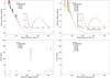 |
Fig. A.1 PIONIER results for the check star υ Cet from 2014 (left) and 2015 (right). |
detector of PIONIER between these epochs. Figure A.1 shows the observed and modeled squared visibility values and closure phases for 2014 and 2015. The low visibility values close to the visibility null and beyond are confirmed to be well consistent with the model atmosphere and to be very accurate. In particular, the visibility values in the second lobe are consistent with the model-predicted strength of the limb-darkening and are significantly different to a uniform disk (UD) function as expected. The measured visibility values in the first lobe with values larger than about 0.2–0.3 lie systematically above the model prediction for both epochs. We interpret this as due to known systematic calibration effects, caused by different magnitudes or airmass between science and calibrator measurements1. This effect is thus also expected for high visibilities of R Scl, and we needed to consider it for our R Scl data as well (see main text). The closure phases show nicely the flip between 0 deg and 180 deg at the position of the visibility minimum. The intermediate values for the spectral channel at 1.59 μm close to a maximum spatial frequency of 230 cycles/arcsec are most likely caused by a flip within the width of the spectral channel. Most closure phase positions are consistent between observed and modeled data. The few deviations may indicate either a diameter that is slightly different to the closure phase data or a variation of the strength of limb-darkening as a function of wavelength that is slightly different between observations and model.
Appendix B: Imaging studies
We studied the effects on the reconstructed R Scl images using different regularization functions, different imaging reconstruction packages with different algorithms, and different start and prior images. In particular, we used all the seven different regularization methods that are available in the IRBis package (Hofmann et al. 2014), including no regularization at all (regularization function 0). For most of the reconstructions, we used a flat prior (regularization functions 1, 3, 4, 5). The remaining regularization functions (2 and 6) require us to use the start image also as a prior image. The regularization functions of IRBis are described in Hofmann et al. (2014), except for regularization functions 5 and 6, which were added later. Regularization function 5 is called “smoothness” and is defined as ![Mathematical equation: \appendix \setcounter{section}{2} \begin{eqnarray*} {\rm H5 }[o_k(x,y)] := \sum_{{\rm d}x,{\rm d}y=-1,1} \sum_{x,y}\frac{{|o_k(x,y)-o_k(x+{\rm d}x,y+{\rm d}y)|^2}}{{\rm prior}(x,y)}\cdot \end{eqnarray*}](/articles/aa/full_html/2017/05/aa30214-16/aa30214-16-eq73.png) Regularization function 6 is called “quadratic Tikhonov” and is defined as:
Regularization function 6 is called “quadratic Tikhonov” and is defined as: ![Mathematical equation: \appendix \setcounter{section}{2} \begin{eqnarray*} {\rm H6}[o_k(x,y)] := \sum_{x,y} |o_k(x,y)-{\rm prior}(x,y)|^2. \end{eqnarray*}](/articles/aa/full_html/2017/05/aa30214-16/aa30214-16-eq74.png) Figure B.1 shows the reconstructed images based on the seven regularization functions (0: no regularization; 1–6: regularization functions 1–6). Table B.1 lists the quality parameters for each of the reconstructions as defined by Hofmann et al. (2014). Here,
Figure B.1 shows the reconstructed images based on the seven regularization functions (0: no regularization; 1–6: regularization functions 1–6). Table B.1 lists the quality parameters for each of the reconstructions as defined by Hofmann et al. (2014). Here,  is the reduced χ2 between the measured and synthetic squared visibility values,
  is the reduced χ2 between the measured and synthetic closure phase values, and ρρ is the ratio between the sum of all positive residuals and the sum of all negative residuals. The quantity qrec adds up the differences from unity of the χ2 and ρρ values, providing one final quality parameter. All reconstructed images as well as the quality parameters are very similar among the different regularization functions. The values are larger than unity because of the known systematic calibration effect described in the main text and in Appendix A, which increases across the three spectral channels at 1.59 μm, 1.68 μm, and 1.76 μm. We chose to use the reconstruction based on regularization function 3 as the final result.
Furthermore, we reconstructed images using two other image reconstruction packages, namely MiRA (Thiébaut 2008) and BSMEM (Buscher 1994). For the MiRA reconstructions, we used smoothness as regularization function, a simple UD fit as a start image, and we used a flat prior image. For the BSMEM reconstruction, we used a two-step approach. We first used the model images as start images to reconstruct a first image that contains only the shorter baselines up to spatial frequencies of about 200 cycles/arcsec. In a second step, we used a smoothed version of the first reconstructions as start images for a final reconstruction based on all data. Figure B.2 shows the resulting reconstructions compared to the final result from IRBis. Again, the resulting images are very similar. Our MiRA reconstruction used double the pixel size compared to our IRBis and BSMEM reconstructions.
In summary, we show that our reconstructed images are robust in view of these variations, which cover in total three different reconstruction packages based on different algorithms, seven different regularization functions including no regularization, different start images, and different priors.
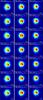 |
Fig. B.1 R Scl image reconstruction based on IRBis with different regularization functions. The image reconstructions are based on (from top to bottom) no regularization function, followed by regularization functions No. 1–6 from Hofmann et al. (2014). |
Quality parameters of the IRBis image reconstructions based on different regularization functions.
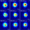 |
Fig. B.2 R Scl image reconstructions based on different image reconstruction packages. For comparison, the top row shows the reconstructions based on IRBis (Hofmann et al. 2014) that we adopted as the final result (as shown in Fig. 9), followed by reconstructions based on (middle row) MiRA (Thiébaut 2008) and (bottom row) BSMEM (Buscher 1994). The MiRA reconstruction uses a UD fit as a start image, smoothness as regularization function, and does not use a prior. The BSMEM reconstruction uses the model atmosphere images as first start images and priors and is based on maximum entropy as regularization function. The MiRA reconstructions use double the pixel size compared to the other two reconstructions. |
All Tables
Quality parameters of the IRBis image reconstructions based on different regularization functions.
All Figures
|
Fig. 1 Visual lightcurve of R Scl based on the AAVSO and AFOEV databases. The solid line represents a sine fit to the ten most recent cycles. The dashed vertical lines denote the mean epochs of our 2012 AMBER and 2014 and 2015 PIONIER observations. |
| In the text | |
|
Fig. 2 AMBER flux spectrum (black) compared to the prediction by the best-fit dynamic model (red). The blue bars denote the mean errors for the first and second halves of the wavelength range. Instrumental and telluric signatures are calibrated and removed. |
| In the text | |
|
Fig. 3 AMBER results (black) compared to the prediction by the best-fit dynamic model (red). The two top panels show the squared visibilities and closure phases versus wavelength for the example of a compact baseline configuration (data set No. 5 in Table 1), followed by an example of an extended configuration (data set No. 9). The blue bars denote the mean errors for the first and second halves of the wavelength range. The three lines correspond to the three baselines of the baseline triplet. |
| In the text | |
|
Fig. 4 AMBER visibility results as a function of baseline length for the examples of bandpasses in the CO (2-0) line at 2.29 μm and the nearby pseudo-continuum at 2.28 μm. The points with error bars denote the observations. The solid lines denote the synthetic visibility based on the best-fit model atmosphere. The fit was derived from the full data set. The green dotted line shows the result based on the uniform disk (UD) fit. The upper panel shows the full visibility range. The lower panel shows an enlargement of the small visibility values at long baselines. |
| In the text | |
|
Fig. 5 The uv coverage obtained for our PIONIER observations of R Scl in 2014 (top) and 2015 (bottom). |
| In the text | |
|
Fig. 6 PIONIER results of R Scl as a function of spatial frequency including the squared visibility values (top) and the closure phases (bottom). The left panels show the results obtained in 2014, and the right panels the results obtained in 2015. The vertical bars indicate the symmetric error bars. The central positions of the measured values are omitted for the sake of clarity. The different colors denote the different spectral channels. The dashed lines indicate the best-fit model atmospheres. For the 2014 data, the synthetic values based on the reconstructed images are shown by horizontal bars. Here, the lower small panels provide the residuals between observations and reconstructed images. |
| In the text | |
|
Fig. 7 Synthetic continuum-normalized spectra using COMA (Aringer et al. 2009) for the most important molecular species and for the full spectrum. The example spectra of this figure are based on the best-fit model snapshot to our first PIONIER epoch. The resolution of the spectra is 1500, except for C3 and C2H2, which are treated in opacity sampling. Also indicated are the three spectral channels of our PIONIER observations, as well as the range of the AMBER MR 2.3 μm mode. |
| In the text | |
|
Fig. 8 Image representations of the intensity profiles of the best-fit dynamic model snapshot. The three images represent the three PIONIER spectral channels with central wavelengths 1.59 μm (left), 1.68 μm (middle), and 1.76 μm (right). All images are based on the same Rosseland angular diameter. The images are convolved with a theoretical point spread function (PSF) using a Gaussian with FWHMλcentral/Bmax. The Rosseland angular diameter is indicated by the dashed black circle. Contours are drawn at levels of 0.9, 0.7, 0.5, 0.3, 0.1. |
| In the text | |
|
Fig. 9 Image reconstructions of R Scl based on our 2014 PIONIER data and the IRBis image reconstruction package (Hofmann et al. 2014). The three images represent the three PIONIER spectral channels with central wavelengths 1.59 μm (left), 1.68 μm (middle), and 1.76 μm (right). The images are convolved with a theoretical point spread function (PSF) using a Gaussian with FWHMλcentral/Bmax. Our estimate of the Rosseland angular diameter is indicated by the dashed black circle. Contours are drawn at levels of 0.9, 0.7, 0.5, 0.3, 0.1. |
| In the text | |
|
Fig. 10 Image reconstructions of R Scl from Fig. 9 divided by the model images from Fig. 8 in order to remove the global center-to-limb intensity variation and to highlight the surface structure on top of this variation. We use a cut-off radius at a model intensity level of 50%, located slightly within the Rosseland radius, which is indicated by the black dashed circle. We calculated the maximum, minimum, and mean intensities inside the cut-off radius to estimate the contrast of the observed structure and printed them on the image. These values are normalized to an average intensity of unity for each spectral channel separately. Contours are drawn at levels of 0.9, 0.7, 0.5. |
| In the text | |
|
Fig. 11 Position of R Scl in the HR diagram together with evolutionary tracks by Lagarde et al. (2012). The tracks are those without rotation and reach up to the start of the TP-AGB. Masses are ZAMS masses; values in parenthesis are masses at the start of the TP-AGB, that is, at the end of the shown tracks. |
| In the text | |
|
Fig. A.1 PIONIER results for the check star υ Cet from 2014 (left) and 2015 (right). |
| In the text | |
|
Fig. B.1 R Scl image reconstruction based on IRBis with different regularization functions. The image reconstructions are based on (from top to bottom) no regularization function, followed by regularization functions No. 1–6 from Hofmann et al. (2014). |
| In the text | |
|
Fig. B.2 R Scl image reconstructions based on different image reconstruction packages. For comparison, the top row shows the reconstructions based on IRBis (Hofmann et al. 2014) that we adopted as the final result (as shown in Fig. 9), followed by reconstructions based on (middle row) MiRA (Thiébaut 2008) and (bottom row) BSMEM (Buscher 1994). The MiRA reconstruction uses a UD fit as a start image, smoothness as regularization function, and does not use a prior. The BSMEM reconstruction uses the model atmosphere images as first start images and priors and is based on maximum entropy as regularization function. The MiRA reconstructions use double the pixel size compared to the other two reconstructions. |
| In the text | |
Current usage metrics show cumulative count of Article Views (full-text article views including HTML views, PDF and ePub downloads, according to the available data) and Abstracts Views on Vision4Press platform.
Data correspond to usage on the plateform after 2015. The current usage metrics is available 48-96 hours after online publication and is updated daily on week days.
Initial download of the metrics may take a while.