© ESO, 2017

1. Introduction

The 3D spatial properties of exoplanet atmospheres are being observed in increasing rate and detail. Two key variables for exoplanet characterisation are the properties of their atmospheric cloud complex and how cloud particle size, compositions, global distributions and opacity affect the resultant observations. A westward offset in the optical phase curves of Kepler-7b was observed by Demory et al. (2013) which was interpreted as cloud particles that backscatter optical photons on the western hemisphere. But a reduced or absent cloud particle abundance on the eastern hemisphere. More Kepler planets (e.g. Kepler-12b, Kepler-8b, Kepler-41b; Angerhausen et al. 2015; Esteves et al. 2015; Shporer & Hu 2015) were found to exhibit similar phase curve behaviour, revealing that offset optical phase curves may be a common feature of hot Jupiter atmospheres. Some Kepler field planets (e.g. HAT-P-7b, Kepler-5b, Kepler-7b, Kepler-17b, Kepler-41b, Keper-76b; Heng & Demory 2013; Angerhausen et al. 2015; Esteves et al. 2015) also have non-negligible geometric albedos (A_g> 0.1) in the Kepler bandpass (0.43−0.89 μm), suggesting the presence of an optical to near-IR scattering aerosol. B band (0.29−0.45 μm) and V band (0.45−0.57 μm) geometric albedo measurements of HD 189733b by Evans et al. (2013) using HST STIS show a blueward slope in the optical, inferring the presence of wavelength-dependent, backscattering cloud particles.

Because of its proximity to its host star, HD 189733b is likely to be tidally locked, with one hemisphere in constant daylight. Infrared flux phase curve observations of HD 189733b using Spitzer (Knutson et al. 2007; Charbonneau et al. 2008; Knutson et al. 2009, 2012; Agol et al. 2010) in photometry bands centred at 3.6 μm, 4.5 μm, 8.0 μm and 24 μm show eastward offsets in peak flux from the sub-stellar point. Global circulation models and radiative-hydrodynamic models of this hot Jupiter (e.g. Showman et al. 2009; Dobbs-Dixon & Agol 2013; Kataria et al. 2016) suggest the development of an equatorial supersonic jet that efficiently advects energy density from the dayside to nightside. Horizontally propagating gravity waves (Watkins & Cho 2010; Perez-Becker & Showman 2013) have also been suggested to contribute to the dayside-nightside energy density advection. These processes result in an east-west hemisphere inhomogeneity in the temperature profiles for HD 189733b, in line with the Spitzer maximum flux offsets.

These observational and modelling investigations suggest that, for cloud forming hot Jupiters, optical and near-IR wavelength instruments such as HST STIS and Kepler are more sensitive to reflected/scattered light from cloud particles in the atmosphere; while longer wavelength IR instruments such as HST WF3, NICOMS, and Spitzer are more sensitive to the thermal emission from the planet itself. Future optical to near-IR wavelength photometry observational programmes such as TESS (Ricker et al. 2014) (0.6−1.0 μm) and CHEOPS (Broeg et al. 2013) (0.4−1.1 μm), will likely characterise a combination of both scattered light and thermal emission for nearby hot Jupiters. Examining data from both of these instruments could therefore provide information about the cloud properties of their atmospheres, similar to studies of the Kepler field planets.

In recent years, theoretical and modelling efforts have explored into exploring how the properties of cloud particles in exoplanet atmospheres affect their observed phase curves and geometric/spherical albedos. Marley et al. (1999) used 1D atmospheric models, combined with a parameterised equilibrium cloud model to predict the albedo spectra of exoplanets. Cahoy et al. (2010) updated and extended the Marley et al. (1999) approach and presented model scattering albedos for Jupiter and Neptune-like exoplanets at different orbital distances from their host stars. Webber et al. (2015) employed a similar method to Cahoy et al. (2010) to model a west-east patchy cloud scenario for Kepler-7b to fit the offset optical phase curve (Demory et al. 2013). Morley et al. (2015) investigated the scattering and thermal emission spectra for photochemical haze and cloud forming Super-Earth atmospheres, comparing their models to the flat transmission spectra of GJ 1214b (Kreidberg et al. 2014). Kopparla et al. (2016) applied a multiple scattering vector radiative transfer scheme to interpret the polarimetry observations of HD 189733b by Wiktorowicz et al. (2015).

Recently, studies using 3D global circulation models (GCMs) have explored modelling the atmospheric reflected light phase curves of Kepler field objects. Oreshenko et al. (2016) performed a GCM experiment using the orbital parameters of Kepler-7b, and applied an equilibrium cloud scheme to model the optical and infrared phase curves offsets of the planet. Parmentier et al. (2016) performed several GCM model experiments over a grid of equilibrium temperatures (T_eq = 1000−2200 K), corresponding to the Kepler hot-Jupiter planet parameter space. They post-processed their model output and applied an equilibrium cloud scheme with a two-stream radiative transfer method to model the reflectivity of clouds across the Kepler bandpass.

Modelling the effects of cloud particles on observable properties of exoplanets using Monte Carlo radiative transfer (MCRT) techniques began with Seager et al. (2000), which mainly focused on producing phase and polarised light curves from a model atmosphere. Hood et al. (2008) applied a parameterised cloud model to a 3D idealised atmosphere of HD 209458b and modelled scattered light curves and geometric albedos of varying cloud heights and scattering properties. de Kok & Stam (2012) used a 3D Monte Carlo scattering code to investigate the influence of forward scattering particles on transit spectroscopy. Garcia Munoz & Isaak (2015) used a Pre-conditioned Backward Monte Carlo method to constrain the cloud particle scattering properties of Kepler-7b. Recently, Monte Carlo transport methods have also been used to model the path and decay of cosmic rays through a Jupiter-like atmosphere (Helling et al. 2016b), important to the ion chemistry in exoplanet atmospheres (Rimmer & Helling 2016).

In this study, we present a 3D Monte Carlo radiative transfer simulation for use in post-processing GCM/RHD atmospheric results with a strong scattering component such as clouds. Our paper outline is as follows; Sect. 2 explains our MCRT model framework and our approach to modelling the HD 189733b atmosphere using MCRT. Section 3 details our model set-up, input quantities and equations for relating the MCRT output to observable quantities. In Sect. 4 we present our model results for scattered and emitted light as well as combining the two components. We also produce Kepler, TESS, and CHEOPS photometric band predictions for HD 189733b based on our simulation output. Section 5 contains the discussion and Sect. 6 summarises key results and conclusions.

2. Approach

We present a MCRT code based on the Hood et al. (2008) model framework, with significant additions and alterations to the scheme to capture a more realistic 3D hot Jupiter atmosphere. In Lee et al. (2016; Paper I in this series) we simulated the atmosphere of HD 189733b using a 3D radiative-hydrodynamic (RHD) model coupled with a self-consistent cloud formation module. In the present paper, we post-process our cloud forming RHD results using the MCRT model to compare our simulation to available observational data and make observational predictions for the TESS and CHEOPS photometric bands.

2.1. MCRT modelling framework

Monte Carlo radiative transfer is a microphysical, stochastic approach to solving radiative transport problems. MCRT simulates the random walk of a luminosity packet (henceforth “L-packet” or “packet”) through a medium and describes the interactions (scattering, absorption) of the packet with the surrounding medium by probabilistic sampling. In MCRT, each initialised packet carries a luminosity fraction ϵ₀/Δt [erg s^-1], proportional to a source (e.g. parent star or planetary atmosphere) of luminosity L_source [erg s^-1]. If NL-packets are initialised by the source of luminosity, the luminosity carried per packet is then (e.g. Lucy 1999) $\frac{{\mathit{ϵ}}_{\mathrm{0}}}{\mathrm{\Delta }\mathit{t}}\mathrm{=}\frac{{\mathit{L}}_{\mathrm{source}}}{\mathit{N}}\mathit{,}$(1)where Δt [s] is the time over which the MCRT experiment is performed; usually Δt = 1 s for time independent MCRT such as the current study. By tracking the proportion of the luminosity of each L-packet that escapes during the simulation in a certain direction, the total luminosity escaping towards a particular observation direction can be found by summing up the contribution of each NL-packet to the total escaping luminosity. If the total luminosity budget in the simulation is normalised to the source luminosity (i.e. L_source = 1), the total contribution of all packets is then the fraction (i.e. f_tot∈ (0, 1)) of source luminosity that escaped the simulation boundaries. To retrieve the luminosity that escaped, the source luminosity is calculated and multiplied by the fraction of luminosity that escaped carried by the L-packets. This is different from numerically solving the radiative transfer equation via, for example, the two-stream approximation (e.g. Toon et al. 1989; Marley & McKay 1999; Fortney et al. 2006) or ray-tracing method (e.g. Rijkhorst et al. 2006). Since MCRT tracks the random walk of a packet and its interactions, radiative transfer through complicated 3D geometries, inhomogeneous opacities, and highly multiple scattering regions can be modelled. MCRT methods have been extensively used to investigate radiative transfer in dusty media, for example, protoplanetary disks (e.g. Whitney et al. 2003; Harries et al. 2004; Pinte et al. 2006; Min et al. 2009), the ISM (e.g. Robitaille 2011) and dusty galactic scale problems (e.g. Wood & Loeb 2000). MCRT has also been applied to the study and retrieval of Earth based cloud properties (e.g. Mayer 2009; Stap et al. 2016). Whitney (2011) and Steinacker et al. (2013) provide a review of MCRT methods and models used for astrophysical-based problems and Mayer (2009) gives details on Earth based applications. The heavily irradiated, inhomogeneous opacity, and thermal structures of cloud forming hot Jupiter atmospheres is an ideal application for a MCRT approach.

The beginning of the MCRT L-packet tracking process starts by stochastically assigning initial starting coordinates and direction of a given packet, depending on the location of the luminosity source that is emitting the packet. For example, a stellar L-packet is initialised randomly at the top of the atmosphere on the dayside of the HD 189733b computational grid in our model. The wavelength-dependent luminosity carried by these stellar packets is the total monochromatic luminosity incident on the atmosphere, divided by the number of simulated packets (ϵ_0,inc/Δt = L_inc,λ/N_inc). The L-packets emitted from the atmosphere itself are assigned a random starting position within a computational cell volume, where the luminosity is proportional to the total monochromatic luminosity of the atmosphere itself (ϵ_0,atm/Δt = L_atm,λ/N_atm). Initialised stellar packets are assumed to travel in a plane-parallel direction towards the planet, while atmospheric, thermally emitted packets are given an isotropic initial direction. The random walk of the L-packet is then determined by stochastically sampling probability distributions that govern the behaviour of the packet (distance travelled, scattering directions etc.).

From the Beer-Lambert law in radiative transfer theory, the probability of a photon packet passing, without interaction, through a medium of total optical depth τ_λ is given by $\mathit{P}\mathrm{\left(}{\mathit{\tau }}_{\mathit{\lambda }}\mathrm{\right)}\mathrm{=}{\mathrm{e}}^{\mathrm{-}{\mathit{\tau }}_{\mathit{\lambda }}}\mathit{,}$(2)where the optical depth τ_λ is defined as ${\mathit{\tau }}_{\mathit{\lambda }}\mathrm{=}{\mathrm{\int }}_{\mathrm{0}}^{{\mathit{l}}_{\max }}{\mathit{\rho }}_{\mathrm{gas}}\mathrm{\left(}\mathit{l}\mathrm{\right)}{\mathit{\kappa }}_{\mathrm{ext}\mathit{,}\mathrm{total}}\mathrm{\left(}\mathit{\lambda ,l}\mathrm{\right)}\mathrm{d}\mathit{l,}$(3)where ρ_gas [g cm^-3] is the local gas density, κ_ext,total [cm² g^-1] (Eq. (26)) the local total extinction opacity, including absorption and scattering, and l [cm] the path length. The probability of a packet interacting with the surrounding medium is then $\mathit{P}\mathrm{\left(}{\mathit{\tau }}_{\mathit{\lambda }}\mathrm{\right)}\mathrm{=}\mathrm{1}\mathrm{-}{\mathrm{e}}^{\mathrm{-}{\mathit{\tau }}_{\mathit{\lambda }}}\mathit{.}$(4)The MCRT method stochastically samples this probability distribution with the use of a (pseudo) random number, P(τ_λ) = ζ∈ [0, 1]. An optical depth, determined stochastically, encountered by the packet before an interaction is given by ${\mathit{\tau }}_{\mathit{\lambda }}\mathrm{=}\mathrm{-}\ln \mathrm{(}\mathrm{1}\mathrm{-}\mathit{\zeta }\mathrm{)}\mathit{.}$(5)Using the definition of τ_λ (Eq. (3)), the distance that the packet travelled through the simulation can then be computed should the density and extinction opacity in the path of the packet be known. After the packet has travelled the distance given by the sampled τ_λ, an interaction with the surrounding medium occurs.

2.2. L-packet interactions with dust and gas

Once the coordinates specified by the optical depth sampling and direction of travel have been reached by the packet, a scattering or absorption event is determined stochastically. In cloud forming hot Jupiter atmospheres, the packet interacts with two components: the gas and cloud particles. An interacting packet exhibits different scattering and absorption behaviours depending what component it is interacting with. The local probability of the packet interacting with the gas phase P_gas is given by ${\mathit{P}}_{\mathrm{gas}}\mathrm{=}\frac{{\mathit{\kappa }}_{\mathrm{ext}\mathit{,}\mathrm{gas}}}{{\mathit{\kappa }}_{\mathrm{ext}\mathit{,}\mathrm{cloud}}\mathrm{+}{\mathit{\kappa }}_{\mathrm{ext}\mathit{,}\mathrm{gas}}}\mathit{,}$(6)where κ_ext,gas [cm² g^-1] is the total opacity of the gas and κ_ext,cloud [cm² g^-1] (defined by Eq. (28)) the total opacity of the cloud component. Should ζ₁<P_gas, (where the indexed random number (e.g. ζ₁, ζ₂) denotes a sequence of random, independent, numbers for a particular scheme) the packet is assumed to interact with the gas phase. The type of interaction, scattering or absorption is determined by sampling the single scattering albedo ω_gas of the gas phase, which is the probability of the packet undergoing a scattering interaction. Since we only consider a H₂ scattering gas component n the MCRT scheme (Sect. 3), the local single scattering albedo of the gas ω_gas is given by ${\mathit{\omega }}_{\mathrm{gas}}\mathrm{=}\frac{{\mathit{\kappa }}_{\mathrm{sca}\mathit{,}{\mathrm{H}}_{\mathrm{2}}}}{{\mathit{\kappa }}_{\mathrm{gas}\mathit{,}\mathrm{ext}}}\mathit{,}$(7)where κ_sca,H2 [cm² g^-1] is the scattering opacity of H₂ and κ_gas,ext = κ_gas,abs + κ_sca,H2 [cm² g^-1] the total extinction for the gas component. Should ζ₂<ω_gas the packet is Rayleigh scattered by H₂, otherwise it is absorbed by the gas phase.

If the interaction is with the cloud component (i.e. ζ₁>P_gas), the type of interaction is given by sampling the local cloud particle single scattering albedo ω_cloud given by ${\mathit{\omega }}_{\mathrm{cloud}}\mathrm{=}\frac{{\mathit{\kappa }}_{\mathrm{scat}\mathit{,}\mathrm{cloud}}}{{\mathit{\kappa }}_{\mathrm{ext}\mathit{,}\mathrm{cloud}}}\mathit{,}$(8)where κ_scat,cloud [cm² g^-1] is the scattering opacity of the cloud particles and κ_ext,cloud [cm² g^-1] the cloud particle total extinction. Should ζ₃<ω_cloud the packet is assumed to be scattered by the cloud component towards a new direction, otherwise it is absorbed by the cloud particles.

After each scattering event, the next interaction location is determined by Eq. (5)and the sampling process is repeated. It is important to note that packets can undergo multiple scattering interactions before getting absorbed, especially in high (ω_gas/cloud> 0.9) single scattering albedo regions.

2.3. Scattering of L-packets by dust and gas

During a scattering event, a new direction of travel is given to the packet, which is dependent on the geometric and compositional properties of the interacting material as well as the wavelength of the interacting packet. A key quantity to consider when modelling a scattering event is the size parameter of the scattering particle given by x = 2πa/λ, where a [cm] is the particle size and λ [cm] the wavelength of the L-packet. The scattering behaviour of an interacting packet can be split into two categories:

• 1.

  x≪ 1 – Rayleigh scattering;

• 2.

  x≳ 1 – Mie scattering.

For Rayleigh scattering, the particle size is magnitudes smaller than the wavelength of light interacting with it, resulting in the well-known double lobed scattering phase function where the probability of scattering in the forward and backward directions are equal. In the Mie regime, the particle size and wavelength of light are of similar magnitudes; the light is typically more forward scattering with a small backscattered component at optical wavelengths. For a scattered packet in MCRT, the new travel direction is generated stochastically from the scattering properties of the interacting material. This is determined by sampling the (normalised) scattering phase function Φ_scat(θ,φ) of the interacting scattering particle, which is the probability of scattering towards angle (θ,φ).

For small cloud particles with small size parameters x≪ 1 and H₂ gas particle scattering, we apply the Rayleigh scattering phase function given by 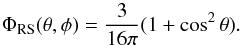${\mathrm{\Phi }}_{\mathrm{RS}}\mathrm{\left(}\mathit{\theta ,\phi }\mathrm{\right)}\mathrm{=}\frac{\mathrm{3}}{\mathrm{16}\mathit{\pi }}\mathrm{(}\mathrm{1}\mathrm{+}{\cos }^{\mathrm{2}}\mathit{\theta }\mathrm{)}\mathit{.}$(9)The θ scattering direction is sampled randomly from this distribution, where a rejection method is applied following the advice in Whitney (2011). The φ scattering angle angle is given by $\mathit{\phi }\mathrm{=}\mathrm{2}\mathit{\pi \zeta ,}$(10)which is a uniform sampling of the φ direction across the 2π radian circular circumference. Rayleigh scattering events are wavelength independent and assumed to be elastic.

When a packet scatters off a cloud particle with size parameter x≳ 1, we apply a Henyey-Greenstein [HG] scattering phase function (Henyey & Greenstein 1941). The HG phase function is an analytic approximation to the Mie scattering phase function, given by ${\mathrm{\Phi }}_{\mathrm{HG}}\mathrm{\left(}{\mathit{g}}_{\mathit{\lambda }}\mathit{,\theta ,\phi }\mathrm{\right)}\mathrm{=}\frac{\mathrm{1}}{\mathrm{4}\mathit{\pi }}\frac{\mathrm{1}\mathrm{-}{\mathit{g}}_{\mathit{\lambda }}^{\mathrm{2}}}{\mathrm{[}\mathrm{1}\mathrm{+}{\mathit{g}}_{\mathit{\lambda }}^{\mathrm{2}}\mathrm{-}\mathrm{2}{\mathit{g}}_{\mathit{\lambda }}\cos \mathit{\theta }{\mathrm{]}}^{\mathrm{3}\mathit{/}\mathrm{2}}}\mathit{,}$(11)where g_λ is the wavelength-dependent scattering asymmetry parameter in the range −1 to 1, given by the results of the Mie theory. This is defined as the mean scattering cosine angle from the relation ${\mathit{g}}_{\mathit{\lambda }}\mathrm{=}\mathrm{⟨}\cos \mathit{\theta }\mathrm{⟩}\mathrm{=}{\mathrm{\int }}_{\mathrm{\Omega }}{\mathrm{\Phi }}_{\mathrm{HG}}\mathrm{\left(}{\mathit{g}}_{\mathit{\lambda }}\mathit{,\theta }\mathrm{\right)}\cos \mathit{\theta }\mathrm{d\Omega }\mathit{.}$(12)A value of g< 0 indicates a preference for packet backscattering, g = 0 an equal backward/forward scattering and g> 0 forward scattering. The scattering angle cosθ is sampled stochastically from this distribution using the following form $\cos \mathit{\theta }\mathrm{=}\frac{\mathrm{1}}{\mathrm{2}{\mathit{g}}_{\mathit{\lambda }}}\left[\mathrm{1}\mathrm{+}{\mathit{g}}_{\mathit{\lambda }}^{\mathrm{2}}\mathrm{-}{\left(\frac{\mathrm{1}\mathrm{-}{\mathit{g}}_{\mathit{\lambda }}^{\mathrm{2}}}{\mathrm{1}\mathrm{-}{\mathit{g}}_{\mathit{\lambda }}\mathrm{+}\mathrm{2}{\mathit{g}}_{\mathit{\lambda }}\mathit{\zeta }}\right)}^{\mathrm{2}}\right]\mathrm{·}$(13)The sampled φ direction is given by Eq. (10). We assume elastic scattering for Mie scattering events. The HG probability distribution has been shown to be a reasonable approximation to Mie scattering within the optical and near-IR wavelength regime (Draine 2003). However, a small but not insignificant probability of backscattering is not completely captured by this approximation at optical wavelengths (e.g. Kattawar 1975; Draine 2003; Hood et al. 2008; Dyudina et al. 2016). To address this, we apply a two-term Henyey-Greenstein (TTHG) function (e.g. Pfeiffer & Chapman 2008; Cahoy et al. 2010; Dyudina et al. 2016) given by ${\mathrm{\Phi }}_{\mathrm{TTHG}}\mathrm{\left(}{\mathit{g}}_{\mathit{a}}\mathit{,}{\mathit{g}}_{\mathit{b}}\mathit{,\theta }\mathrm{\right)}\mathrm{=}\mathit{\alpha }{\mathrm{\Phi }}_{\mathrm{HG}}\mathrm{\left(}{\mathit{g}}_{\mathit{a}}\mathit{,\theta }\mathrm{\right)}\mathrm{+}\mathit{\beta }{\mathrm{\Phi }}_{\mathrm{HG}}\mathrm{\left(}{\mathit{g}}_{\mathit{b}}\mathit{,\theta }\mathrm{\right)}\mathit{,}$(14)where α is the mainly forward scattering component with g_a> 0, and β a mainly backscattering component with g_b< 0. For all parameters, the relation α + β = 1 has to be satisfied. We apply the parameters in Cahoy et al. (2010) where g_a = g_λ, g_b = −g_λ/2 and α = $\mathrm{1}\mathrm{-}{\mathit{g}}_{\mathit{b}}^{\mathrm{2}}$, β = ${\mathit{g}}_{\mathit{b}}^{\mathrm{2}}$. The TTHG form is commonly used in various atmospheric radiative transfer scattering codes (e.g. Marley et al. 1999; Cahoy et al. 2010; Barstow et al. 2014; Garcia Munoz & Isaak 2015; Dyudina et al. 2016) and more qualitatively captures the Mie backscattering lobe at optical wavelengths.

To determine the scattering angle of a TTHG event, the probability of forward scattering is simply given by ζ<α (Pfeiffer & Chapman 2008) after which Eq. (13)with g_λ = g_a can be used, otherwise the scattering is a backscattering event in which g_λ = g_b is applied. Although α and β are used to determine a forward or backward scattering event, due to the probabilistic sampling of the HG function scattering angle, sampling the α term does not necessarily always result in a forward scattering event, nor β a backward scattered event.

Since there is a distribution of cloud particle sizes in each cell, the size of an individual cloud particle interacting with the packet must be stochastically determined from the size distribution properties. This is required as the size distribution may contain a combination of cloud particles in the Rayleigh and Mie size parameter regimes, resulting in a mixture of packet scattering behaviour. To capture this scattering behaviour, we perform a stochastic sampling from the cumulative distribution function (CDF) of the size distribution, which is the fractional contribution of each particle size to the total area of the particle ensemble. The area distribution is used, rather than the size distribution, as this better captures the contribution of each cloud particle radius to the scattering cross-sectional opacity of the size distribution (since κ_sca ∝ f(a)a², Eq. (28)). The cloud particle mean grain size, ⟨ a ⟩ [cm], and mean grain area, ⟨ A ⟩ [cm²], of the cloud particles in each RHD cell can be found from the dust moment values, L_j (Woitke & Helling 2003, 2004; Lee et al. 2015). Assuming an arithmetic log-normal distribution of cloud particle sizes (e.g. Ackerman & Marley 2001), the mean μ and standard deviation σ (more specifically their natural logarithms) of the ensemble of particles in each cell is then calculated (e.g. Stark et al. 2015). The surface area log-normal distribution is given by (e.g. Heintzenberg 1994) $\mathit{A}\mathrm{\left(}\mathit{a}\mathrm{\right)}\mathrm{=}\frac{{\mathit{A}}_{\mathrm{0}}}{\mathit{a}{\mathit{\sigma }}_{\mathit{A}}\sqrt{\mathrm{2}\mathit{\pi }}}\exp \left[\mathrm{-}\frac{\mathrm{\left(}\ln \mathrm{\right(}\mathit{a}\mathrm{)}\mathrm{-}{\mathit{\mu }}_{\mathit{A}}{\mathrm{)}}^{\mathrm{2}}}{\mathrm{2}{\mathit{\sigma }}_{\mathit{A}}^{\mathrm{2}}}\right]$(15)which is the log-normal size distribution multiplied by the surface area 4πa², with the total area A₀ = 4πn_dexp(2μ + 2σ²) (e.g. Zender 2015), where a [cm] is the sampled grain size, n_d [cm^-3] the total cloud particle number density, μ_A the arithmetic mean of the area distribution and σ_A the standard deviation of the area distribution. The relation between the mean and standard deviation of the size distribution (μ,σ) and area distribution (μ_A,σ_A) are given by (e.g. Heintzenberg 1994)

$\begin{array}{ccc}& & {\mathit{\mu }}_{\mathit{A}}\mathrm{=}\mathit{\mu }\mathrm{+}\mathrm{2}{\mathit{\sigma }}^{\mathrm{2}}\mathit{,}\\ & & {\mathit{\sigma }}_{\mathit{A}}\mathrm{=}\mathit{\sigma }\mathit{.}\end{array}$(16)The cloud particle area cumulative distribution function of the log-normal size distribution A_CDF∈ (0, 1) is then constructed in each cell from (e.g. Zender 2015) ${\mathit{A}}_{\mathrm{CDF}}\mathrm{\left(}\mathit{a}\mathrm{\right)}\mathrm{=}\frac{\mathrm{1}}{\mathrm{2}}\mathrm{+}\frac{\mathrm{1}}{\mathrm{2}}\mathrm{erf}\left[\frac{\ln \mathrm{\left(}\mathrm{a}\mathrm{\right)}\mathrm{-}{\mathit{\mu }}_{\mathrm{A}}}{\sqrt{\mathrm{2}}{\mathit{\sigma }}_{\mathrm{A}}}\right]\mathit{,}$(17)where erf is the error function. We construct A_CDF for 100 log-spaced cloud particle size a bins between a minimum seed particle size a_seed~ 0.001 μm and a maximum of a_max = 10 ·a_effμm, where a_eff is the effective cloud particle radius (Eq. (29)). During the simulation, by sampling a random number ζ∈ (0, 1), the particle size from the distribution interacting with the packet can therefore be stochastically determined by sampling A_CDF (i.e. ζ→a).

We assume two scattering regime limits in our model for a certain cloud particle size parameter (x = 2πa/λ). For x< 0.1 we assume a Rayleigh scattering event, while if x≥ 0.1 we assume a TTHG scattering event. We assume TTHG scattering events to occur at the properties of the effective mean radius values (e.g. g_λ(a_eff), Sect. 3.2). The effect of this scheme is that if the mean and variance skew the area distribution towards larger cloud particle sizes, then the fractional contribution of particle areas where x≥ 0.1 increases, and so the probability of a TTHG event is increased. However, if the distribution is skewed towards smaller cloud particle sizes then a greater fraction of cloud particle area satisfies x< 0.1, increasing the likelihood of a Rayleigh event.

2.4. MCRT variance reduction techniques

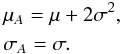
Fig. 1 Incident scattered (left) and atmospheric emitted (right) light image array of the L-packet luminosity fractions fx,y(λ,α) ∈ (0, 1) escaping from the HD 189733b simulation. These images are produced by the next event estimator method at 1.0 μm for a viewing angle/phase of α = 60° (eastern dayside). The sharp transition from blue to black at pixel numbers x = 120−150 is the eastern terminator in the scattered light image, including a “twilight” effect where packets scatter past the terminator line. The effect of the grid structure on the images is more apparent in the emitted light, since packets are initialised from within the cell volumes.

In a basic MCRT scheme, to produce observable quantities for a particular observation direction, the MCRT code would track how many packets of a particular luminosity entered the simulation and how many escaped. The ratio of these values would then give the fraction of luminosity escaping the simulation domain towards a particular direction. However, the probability of an individual packet escaping by chance towards a particular direction can be incredibly small, depending on the geometric properties of the simulation, and can produce noisy results if not enough Monte Carlo packets are simulated (e.g. see Dupree & Fraley 2002). Therefore, variance reduction techniques were developed for MCRT, which allows for a much improved signal to noise and greater computational efficiency than the basic scheme. We employ three techniques in this study as follows: next event estimation, survival biasing, and composite emission biasing. The variance and convergence properties our model output is presented in Sect. 4.5.

2.4.1. Next event estimation

Next event estimation (e.g. Yusef-Zadeh et al. 1984; Wood & Reynolds 1999) is a variance reduction method that uses a ray-tracing technique in conjunction with the Monte Carlo scheme. At every scattering or emission event, a fraction of the packet’s luminosity, W_poϵ₀, (Eq. (1)) is peeled off towards an observation direction using a ray-tracing method. The fraction of luminosity is given by the normalised phase function of the type of interaction, weighted by the probability of the packet escaping the simulation towards this observation direction. The peeled off luminosity is wavelength dependent and the luminosity carried by the packet is not altered in the peeling off scheme. The peeled off luminosity is then stored in a 2D pixel image array at this observation direction, which can be used to derive observational quantities.

Multiple pixel images can be constructed for many viewing angles and wavelengths, which allows a single photon packet interaction to contribute to multiple output images at different planetary phases. Since every packet now contributes to the output images, this improves the signal to noise of the output as images can be produced without relying on packets emerging by chance from the simulation boundaries towards the observer. Figure 1 illustrates the resultant next event estimator scattered stellar (left) and atmospheric emitted (right) luminosity fractions at 1.0 μm for a viewing angle of φ = 60°, θ = 0°.

For atmospheric emission, assumed to be isotropic, the fraction of the packet luminosity peeled off towards observation direction α is given by ${\mathit{W}}_{\mathrm{po}}\mathrm{\left(}\mathit{\alpha }\mathrm{\right)}\mathrm{=}\frac{\mathrm{1}}{\mathrm{4}\mathit{\pi }}{\mathrm{e}}^{\mathrm{-}{\mathit{\tau }}_{\mathrm{2}}}\mathit{,}$(18)where 1/4π is the normalisation factor for isotropic emission into 4π steradians and τ₂(λ) (where indexed τ terms (e.g. τ₁,τ₂ etc.) indicate optical depths calculated using the ray-tracing method to the simulation boundaries, and non-indexed τ denotes the stochastically sampled optical depth for photon packets) the optical depth through the computational zone at wavelength λ, towards the observational direction.

For non-isotropic scattering events such as Rayleigh or Henyey-Greenstein scattering, the fraction of peeled off luminosity is related to the probability of the packet scattering towards the observational direction. For Rayleigh scattering, the weight of peeled off luminosity is given by ${\mathit{W}}_{\mathrm{po}}\mathrm{\left(}\mathit{\alpha }\mathrm{\right)}\mathrm{=}{\mathrm{\Phi }}_{\mathrm{RS}}\mathrm{\left(}\mathit{\alpha }\mathrm{\right)}{\mathrm{e}}^{\mathrm{-}{\mathit{\tau }}_{\mathrm{2}}}\mathit{,}$(19)and for two-term Henyey-Greenstein, ${\mathit{W}}_{\mathrm{po}}\mathrm{\left(}\mathit{\alpha }\mathrm{\right)}\mathrm{=}{\mathrm{\Phi }}_{\mathrm{TTHG}}\mathrm{\left(}{\mathit{g}}_{\mathit{a}}\mathit{,}{\mathit{g}}_{\mathit{b}}\mathit{,\alpha }\mathrm{\right)}{\mathrm{e}}^{\mathrm{-}{\mathit{\tau }}_{\mathrm{2}}}\mathit{.}$(20)Phase curve information can be calculated by adding the contribution of each event to an image in the desired observation direction (e.g. 360° in longitude). Each weight is added into a square image pixel array of (x,y) = (201, 201) pixels and then normalised by the number of initialised packets after the simulation is complete. The luminosity scattered/emitted in the observational direction can then be found by multiplying the fraction of escaping luminosity by the total luminosity of the emitting source.

2.4.2. Survival biasing

For diffuse emission from within the simulation boundaries, the packet is forced to scatter at each interaction and not terminated upon absorption (see Sect. 3). In order to conserve energy, the weight of the luminosity carried by the packet is reduced at each interaction by the single scattering albedo ${\mathit{W}}_{\mathrm{new}}\mathrm{=}\mathit{\omega W,}$(21)where, in an interaction with the gas phase, ω = ω_gas (Eq. (7)) and with the cloud particles ω = ω_cloud (Eq. (8)). The fraction of luminosity lost by the photon packet due to absorption is then taken into account in the peeled off images as the packet interacts with the surrounding medium. So that a packet does not scatter indefinitely with ever decreasing weight, a Russian Roulette scheme (e.g. Dupree & Fraley 2002) is applied to stochastically terminate packets below a predefined weight cut-off. The packet is then given a 1 in 10 chance of surviving, with the new weight of the surviving packets W_new = 10 ·W. In our model, packets with weight W< 10^-3 are entered into the Russian Roulette scheme.

2.4.3. Composite emission biasing

For hot Jupiter atmospheres, the total dayside emission luminosity can be orders of magnitude greater than the emission from the nightside of the planet. In non-biased MCRT, the number of packets N_i,λ emitted from cell i is given by the fraction of the luminosity of the cell to the total luminosity of the atmospheric cells at this wavelength (e.g. Pinte et al. 2006), ${\mathit{N}}_{\mathit{i,\lambda }}\mathrm{=}\frac{{\mathit{L}}_{\mathit{i,\lambda }}}{{\sum }_{\mathit{i}}{\mathit{L}}_{\mathit{i,\lambda }}}{\mathit{N}}_{\mathrm{atm}}\mathit{,}$(22)where L_i,λ is the luminosity of the cell, ∑ _iL_i,λ the total luminosity of the considered cells, and N_atm the total number of atmospheric L-packets emitted at wavelength λ. Low luminosity regions (e.g. the nightside), where L_i,λ ≪ ∑ _iL_i,λ can therefore be under sampled in the emission scheme, which increases the variance of results derived from these regions.

To address this, we implement the multiple component, emission composite biasing method from Baes et al. (2016), where a linear combination of the unbiased emission (Eq. (22)) probability distribution function and a uniform (in cell number) distribution function is applied. This results in the number of emitted packets per cell given by ${\mathit{N}}_{\mathit{i,\lambda }}\mathrm{=}{\mathit{N}}_{\mathrm{atm}}\left[\mathrm{(}\mathrm{1}\mathrm{-}\mathit{\eta }\mathrm{)}\frac{{\mathit{L}}_{\mathit{i,\lambda }}}{{\sum }_{\mathit{i}}{\mathit{L}}_{\mathit{i,\lambda }}}\mathrm{+}\frac{\mathit{\eta }}{{\sum }_{\mathit{i}}{\mathit{i}}_{\mathit{\lambda }}}\right]\mathit{,}$(23)where η∈ (0, 1), is a parameter governing the linear combination and ∑ _ii_λ the total number emitting cells at wavelength λ. To conserve the total luminosity, each emitted packet is given a cell dependent starting weight of ${\mathit{W}}_{\mathrm{em}}\mathrm{=}\frac{\mathrm{1}}{\mathrm{(}\mathrm{1}\mathrm{-}\mathit{\eta }\mathrm{)}\mathrm{+}\mathit{\eta }\mathrm{⟨}{\mathit{L}}_{\mathit{i,\lambda }}\mathrm{⟩}\mathit{/}{\mathit{L}}_{\mathit{i,\lambda }}}\mathit{,}$(24)where $\mathrm{⟨}{\mathit{L}}_{\mathit{i,\lambda }}\mathrm{⟩}\mathrm{=}\frac{{\sum }_{\mathit{i}}{\mathit{L}}_{\mathit{i,\lambda }}}{{\sum }_{\mathit{i}}{\mathit{i}}_{\mathit{\lambda }}}\mathit{,}$(25)is the average cell luminosity at wavelength λ. We apply a fixed η = 0.5 throughout our simulations. Baes et al. (2016) provide an in depth description of this composite emission biasing method.

3. Input and output quantities

In this section, we provide details of our input quantities to the MCRT scheme and the relationships between the MCRT output, which is in normalised luminosity fraction units, and observational quantities (geometric albedos, flux ratios, etc.). We perform all scattering and emission calculations for 250 wavelengths in the range 0.3 and 5.0 μm, linear in wave-number space. Table 1 shows the HD 189733 star and planet parameters used in the simulation.

3.1. Summary of 3D RHD results

We briefly provide a summary of the results of our 3D cloud forming RHD simulation of HD 189733b (Paper I), which are used as input to the MCRT post-processing simulation. The mean cloud particle sizes in the upper atmosphere (0.1–100 mbar) range from seed particle sizes ⟨ a ⟩~ 0.001 μm at the hottest regions of the dayside to ⟨ a ⟩~ 0.1 μm at higher latitudes and the cooler nightside. Cloud particles to the east of the sub-stellar point are generally smaller than those to the west of the sub-stellar point, with ~1 order of magnitude differences between cloud particle sizes at the east and west terminator regions. Cloud particle composition also varies with latitude and longitude; TiO₂[s] rich grains dominate the hotter dayside equatorial regions, while silicate materials (SiO[s], SiO₂[s], MgSiO₃[s], Mg₂SiO₄[s]) dominate the cooler higher latitudes and nightside regions. TiO₂[s] rich grains are also more prevalent on the eastern terminator region, while silicates dominate the western regions. This material composition disparity, due to differences in the thermal stability between TiO₂[s] and silicates, is the main reason why each terminator region contains different cloud particle sizes.

For the MCRT post-processing simulation, we use the same spherical RHD simulation dimensions of radial, longitude and latitude sizes (R, φ, θ) = (100, 160, 64) respectively. Latitude θ cells defined near the pole edges in the RHD simulation are assumed to extend to −π and π radians respectively. This is required so that no regions remain undefined across the whole sphere in the MCRT simulation. Cell thermodynamic quantities (T_gas, ρ_gas) and cloud moment properties (L_j) are taken from the snapshot (~60 Earth days) simulation of Paper I. The cell thermodynamic states are kept constant at the values given by the RHD model throughout the MCRT simulations.

3.2. Cloud and gas opacity

The input opacities are critical to the accuracy of the MCRT scheme as they govern the distance travelled by the stochastically sampled τ_λ, the probability of packets scattering, and the type of scattering events. The total extinction opacity κ_ext,total [cm² g^-1] in each cell is given by ${\mathit{\kappa }}_{\mathrm{ext}\mathit{,}\mathrm{total}}\mathrm{=}{\mathit{\kappa }}_{\mathrm{abs}\mathit{,}\mathrm{gas}}\mathrm{+}{\mathit{\kappa }}_{\mathrm{sca}\mathit{,}{\mathrm{H}}_{\mathrm{2}}}\mathrm{+}{\mathit{\kappa }}_{\mathrm{ext}\mathit{,}\mathrm{cloud}}\mathit{,}$(26)where κ_abs,gas [cm² g^-1] is the absorption due to gaseous atoms and molecules, κ_sca,H2 [cm² g^-1] is the contribution of Rayleigh scattering by molecular H₂, and κ_ext,cloud = κ_abs,cloud + κ_scat,cloud is the total extinction (absorption + scattering) due to cloud particles.

For gas absorption opacities κ_abs,gas, we adopt the solar metallicity, chemical equilibrium Sharp & Burrows (2007) opacity tables, without TiO and ViO opacities, linearly interpolated to the RHD cell thermodynamic properties. We perform k-distribution (e.g. Goody et al. 1989; Lacis & Oinas 1991; Grimm & Heng 2015) band averages from the high-resolution opacity tables across 250 bins, linear in wave-number between (wavelengths) 0.3 and 5 μm. Eight Gaussian quadrature points were used with a split at 95% of the cumulative opacity, in the same manner as Showman et al. (2009).

For the H₂ scattering opacity we use the cross-section, wavelength relation from Dalgarno & Williams (1962) given by ${\mathit{\sigma }}_{\mathrm{sca}\mathit{,}{\mathrm{H}}_{\mathrm{2}}}\mathrm{\left(}\mathit{\lambda }\mathrm{\right)}\mathrm{=}\frac{\mathrm{8.14}\mathrm{\times }{\mathrm{10}}^{-13}}{{\mathit{\lambda }}^{\mathrm{4}}}\mathrm{+}\frac{\mathrm{1.28}\mathrm{\times }{\mathrm{10}}^{-6}}{{\mathit{\lambda }}^{\mathrm{6}}}\mathrm{+}\frac{\mathrm{1.61}}{{\mathit{\lambda }}^{\mathrm{8}}}\mathit{,}$(27)where λ is in Å and σ_sca,H2 in cm². This is converted into a mass opacity by the relation κ_sca,H2(λ) = n_H2σ_sca,H2(λ)/ρ_gas. The abundance of molecular H₂ (n_H2 [cm^-3]) is calculated at each cell assuming chemical equilibrium using the routines from Helling et al. (2016a).

For cloud particle absorption and scattering opacities we calculate a mono-disperse absorption κ_abs,cloud and scattering κ_sca,cloud opacity of the cloud particles in each cell given by

$\begin{array}{ccc}& & {\mathit{\kappa }}_{\mathrm{abs}\mathit{,}\mathrm{cloud}}\mathrm{\left(}\mathit{\lambda }\mathrm{\right)}\mathrm{=}\mathit{\pi }{\mathit{a}}^{\mathrm{2}}{\mathit{Q}}_{\mathrm{abs}}\mathrm{\left(}\mathit{\lambda ,a}\mathrm{\right)}{\mathit{n}}_{\mathrm{d}}\mathit{/}{\mathit{\rho }}_{\mathrm{gas}}\mathit{,}\\ & & \end{array}$(28)respectively, where a [cm] is cloud particle size, Q_abs and Q_sca are the absorption and scattering efficiency factors given by the MieX code of Wolf & Voshchinnikov (2004), and n_d [cm^-3] is the total cloud particle number density. We calculate the cloud opacities at the effective grain size, a_eff, which is given by the ratio of the third (L₃) and second (L₂) cloud moments (Hansen & Travis 1974) ${\mathit{a}}_{\mathrm{eff}}\mathrm{=}\mathrm{3}\sqrt{\frac{\mathrm{3}}{\mathrm{4}\mathit{\pi }}}\frac{{\mathit{L}}_{\mathrm{3}}}{{\mathit{L}}_{\mathrm{2}}}\mathit{,}$(29)which is the area weighted average cloud particle size across the grain size distribution. The single scattering albedo ω_cloud (Eq. (8)) and scattering asymmetry parameter g_λ (Eq. (12)) are also calculated at the effective cloud particle size. Effective (n,k) coefficients of the cloud particles required as input for Mie theory are calculated for mixed material cloud particles using effective medium theory in the same way as Lee et al. (2015).

3.3. Scattered light phase curves and albedo spectra

Fig. 2 Diagram visualising the definition of equatorial viewing angle α [°] used in this study. Viewing angles east of the sub-stellar point are positively defined, while regions west of the sub-stellar point are negatively defined.

To produce scattered light phase curves, we track the random walks of stellar L-packets incident on the HD 189733b simulated atmosphere. The stellar illumination is assumed to be plane parallel from the direction of the host star, with the initial latitude and longitude (φ, θ) top of atmosphere positions determined stochastically from a rejection method, carried out across the circular annulus of the dayside face of the planet. In this mode, should the packet be absorbed by the gas or cloud particles, it is terminated and no longer contributes to the simulation. The survival biasing variance reduction technique is not required in this mode since the majority of incident stellar packets are scattered or absorbed in the atmosphere. Therefore, the fractional weight of the packet luminosity remains unchanged in this mode (W = 1). We chose a viewing angle of θ = 0° latitude (equator) while altering the longitude viewing angle α to capture planetary phase information. We define α = 0° as the viewing angle at the sub-stellar point (i.e.. full phase) with +°α eastward and −°α westward from the sub-stellar point. Figure 2 shows a schematic visualisation of this α definition. As a consequence, we ignore possible viewing effects of non-negligible transit impact parameters, similar to other post-processing RHD/GCM methods (e.g. Fortney et al. 2006; Showman et al. 2009; Amundsen et al. 2016).

The total fraction of luminosity, carried by the photon packets, escaping towards viewing angle α at wavelength λ is given by summing the image pixel array produced by the peeling off method (Sect. 2.4.1, Fig. 1) ${\mathit{f}}_{\mathrm{total}}\mathrm{\left(}\mathit{\lambda ,\alpha }\mathrm{\right)}\mathrm{=}\sum _{\mathit{x,y}}{\mathit{f}}_{\mathit{x,y}}\mathrm{\left(}\mathit{\lambda ,\alpha }\mathrm{\right)}\mathit{,}$(30)where f_total is the total fraction of luminosity escaping towards viewing angle α at wavelength λ and f_x,y is the fraction of luminosity contained in a (x,y) pixel image array. The monochromatic phase dependent albedo A_λ(α) is defined as ${\mathit{A}}_{\mathit{\lambda }}\mathrm{\left(}\mathit{\alpha }\mathrm{\right)}\mathrm{=}\frac{{\mathit{f}}_{\mathrm{total}}\mathrm{\left(}\mathit{\lambda ,\alpha }\mathrm{\right)}{\mathit{L}}_{\mathrm{inc}}\mathrm{\left(}\mathit{\lambda }\mathrm{\right)}}{{\mathit{L}}_{\mathrm{inc}}\mathrm{\left(}\mathit{\lambda }\mathrm{\right)}}\mathrm{=}{\mathit{f}}_{\mathrm{total}}\mathrm{\left(}\mathit{\lambda ,\alpha }\mathrm{\right)}\mathit{,}$(31)where L_inc [erg s^-1] is the incident luminosity onto the dayside face of the exoplanet atmosphere from the host star. The monochromatic apparent geometric albedo A_g,λ is defined as the fraction of scattered light at zero phase angle (α = 0°) to an equivalent spherical Lambertain surface (e.g. Seager 2010; Madhusudhan & Burrows 2012). In the MCRT scheme A_g,λ is derived from the luminosity fractions by the equation ${\mathit{A}}_{\mathrm{g}\mathit{,\lambda }}\mathrm{=}\frac{{\mathit{f}}_{\mathrm{total}}\mathrm{(}\mathit{\lambda ,\alpha }\mathrm{=}\mathrm{0}°\mathrm{)}{\mathit{L}}_{\mathrm{inc}}\mathrm{\left(}\mathit{\lambda }\mathrm{\right)}}{{\mathit{f}}_{\mathrm{Lambert}}{\mathit{L}}_{\mathrm{inc}}\mathrm{\left(}\mathit{\lambda }\mathrm{\right)}}\mathrm{=}\frac{{\mathit{f}}_{\mathrm{total}}\mathrm{(}\mathit{\lambda ,\alpha }\mathrm{=}\mathrm{0}°\mathrm{)}}{\mathrm{2}\mathit{/}\mathrm{3}}\mathit{,}$(32)where f_Lambert = 2/3 is the scattering fraction of the theoretical Lambertian planet at zero phase.

The wavelength-dependent classical phase function (e.g. Seager 2010; Madhusudhan & Burrows 2012) can be constructed from the scattering fractions ${\mathrm{\Phi }}_{\mathit{\lambda }}\mathrm{\left(}\mathit{\alpha }\mathrm{\right)}\mathrm{=}\frac{{\mathit{f}}_{\mathrm{total}}\mathrm{\left(}\mathit{\lambda ,\alpha }\mathrm{\right)}}{{\mathit{f}}_{\mathrm{total}}\mathrm{(}\mathit{\lambda ,\alpha }\mathrm{=}\mathrm{0}°\mathrm{)}}\mathit{,}$(33)which is the ratio of reflected luminosity at viewing angle α compared to the fraction reflected at α = 0°. The monochromatic planetary luminosity due to reflected starlight L_p,scat,λ [erg s^-1 cm^-1] as a function of viewing angle is given by ${\mathit{L}}_{\mathrm{p}\mathit{,}\mathrm{scat}\mathit{,\lambda }}\mathrm{\left(}\mathit{\alpha }\mathrm{\right)}\mathrm{=}{\mathit{f}}_{\mathrm{total}}\mathrm{\left(}\mathit{\lambda ,\alpha }\mathrm{\right)}{\mathit{L}}_{\mathit{\star }\mathit{,\lambda }}\left(\frac{{\mathit{R}}_{\mathit{p}}^{\mathrm{2}}}{\mathrm{4}{\mathit{a}}^{\mathrm{2}}}\right)\mathit{,}$(34)where R_p is the radius of the planet and a the semi-major axis. The monochromatic luminosity of the star is given by ${\mathit{L}}_{\mathit{\star }\mathit{,\lambda }}\mathrm{=}\mathrm{4}{\mathit{\pi }}^{\mathrm{2}}{\mathit{R}}_{\mathit{\star }}^{\mathrm{2}}{\mathit{B}}_{\mathit{\lambda }}\mathrm{\left(}{\mathit{T}}_{\mathit{\star }\mathit{,}\mathrm{eff}}\mathit{,\lambda }\mathrm{\right)}\mathit{,}$(35)where R_⋆ is the radius of the star and B_λ the Planck function, which is dependent on the stellar effective temperature T_⋆,eff. To ensure good signal to noise, we emit the same number of packets (N_inc = 10⁷) for each (pseudo) monochromatic wavelength.

3.4. Emitted light phase curves and spectra

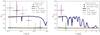Fig. 3 Scattered light apparent geometric albedo Ag,λ (Eq. (32)) of our HD 189733b simulation output compared to Evans et al. (2013)’s individual HST STIS measurements. The total contribution is indicated by the solid blue line; TTHG cloud particle scattering by the dashed orange line; Rayleigh cloud particle scattering by the teal dash-dotted line; H2 Rayleigh scattering by the brown solid line. Left (0.29−0.6 μm): the Rayleigh and TTHG model is generally consistent with the B band HST STIS measurements, but does not predict the low albedo of the V band. Right (0.29−5 μm): extended spectra from 0.3−5 μm, showing the convolved B band and V band measurements from Evans et al. (2013). Ag,λ becomes negligible beyond 5 μm.

We follow a similar scheme to the protoplanetary disk and ISM MCRT based studies of Pinte et al. (2006) and Robitaille (2011) where the monochromatic luminosity L_i,λ [erg s^-1 cm^-1] of computational cell i is ${\mathit{L}}_{\mathit{i,\lambda }}\mathrm{=}\mathrm{4}\mathit{\pi }{\mathit{\rho }}_{\mathit{i,}\mathrm{gas}}{\mathit{V}}_{\mathit{i}}\mathrm{(}{\mathit{\kappa }}_{\mathit{i,\lambda ,}\mathrm{abs}\mathit{,}\mathrm{cloud}}\mathrm{+}{\mathit{\kappa }}_{\mathit{i,\lambda ,}\mathrm{abs}\mathit{,}\mathrm{gas}}\mathrm{)}{\mathit{B}}_{\mathit{\lambda }}\mathrm{\left(}{\mathit{T}}_{\mathit{i}}\mathrm{\right)}\mathit{,}$(36)where V_i is the volume of the cell, ρ_i,gas the gas density, κ_{i,λ,abs,cloud} the cloud absorption opacity, κ_i,λ,abs,gas the gas absorption opacity, and B_i,λ the Planck function, which is dependent on the cell temperature T_i.

In this scheme the packets are not terminated upon absorption but are forced to scatter with reduction in their weight at each event. Survival biasing and Russian Roulette techniques are therefore applied (Sect. 2.4.2). Composite emission biasing is also applied to decrease the noise error of results derived from nightside regions (Sect. 2.4.3). We employ a wavelength-dependent dark zone (Pinte et al. 2006) of longitude- and latitude-dependent, radially integrated optical depth τ_r,λ(θ,φ) = 30 (Eq. (3)). No packets are emitted from these regions and packets are terminated if they cross into regions deeper in the atmosphere than the cell radial index given by this condition. This prevents tracking packets through low luminosity weight regions which contribute negligibly to the photospheric emission. The contribution of cells below this depth to the total cell emission luminosity is also ignored (i.e. L_i,λ = 0). The emitted monochromatic luminosity L_p,em,λ [erg s^-1 cm^-1] from the planet at viewing angle α is then given by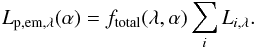${\mathit{L}}_{\mathrm{p}\mathit{,}\mathrm{em}\mathit{,\lambda }}\mathrm{\left(}\mathit{\alpha }\mathrm{\right)}\mathrm{=}{\mathit{f}}_{\mathrm{total}}\mathrm{\left(}\mathit{\lambda ,\alpha }\mathrm{\right)}\sum _{\mathit{i}}{\mathit{L}}_{\mathit{i,\lambda }}\mathit{.}$(37)As in the scattered light case, we assume the same number of packets (N_atm = 10⁸) for each (pseudo) monochromatic wavelength.

4. Results

In this section, we present the scattered and emitted light results of our MCRT post-processing method. We chose 36 different viewing angles to capture orbital phase information of the scattered and emitted light, which gives a phase resolution of Δα = 10°. Sections 4.1 and 4.2 present our incident scattered light apparent geometric albedo A_g, and albedo spectra/phase curves, respectively. Section 4.3 presents our atmospheric emitted luminosity spectra and phase curves. In Sect. 4.4 we combine our scattered and emitted light results and compare these combined results with current observations; we also predict Kepler, TESS and CHEOPS photometric observations for HD 189733b. Finally, in Sect. 4.5 we discuss the variance and convergence properties of our MCRT model results.

4.1. Geometric albedo

Figure 3 shows the resultant geometric albedo of our post-processed cloud forming HD 189733b 3D RHD model, which we compare to the HST STIS observations of Evans et al. (2013). Our results in the B band are consistent with the individual STIS data points, but underestimate the convolved B band geometric albedo. Our results are also consistent with the Wiktorowicz et al. (2015) ground based B + V band polarimetry measurement of an upper limit of A_g,λ< 0.4. Our V band result compares poorer to the observations, however it is clear that Na absorption is responsible for the downward trend near 0.6 μm. This is perhaps because of the presence of an unknown absorbing material in the V band (Sect. 5).

Figure 3 also shows the individual contributions from H₂ Rayleigh scattering, cloud particle Rayleigh scattering, and cloud particle TTHG scattering to the total fractions. The TTHG scattering contributes the greatest fraction to the total geometric albedo across all wavelengths. A small H₂ Rayleigh scattering component is also present at shorter optical wavelengths.

4.2. Scattered light phase curves

During a single orbit of HD 189733b around its parent star, different atmospheric regions come in and out of view of the detector, dependent on the planetary phase being observed. If eastward and westward hemispheres of the dayside atmospheric properties are different, an asymmetric signal as a function of phase (α) is expected to be observed. In order to extract this phase behaviour from our 3D RHD results, we produce observables at various viewing angles (longitude from the sub-stellar point) α during the Monte Carlo simulation.

Figure 4 shows the albedo A_λ(α) spectra (Eq. (31)) as a function of phase. Slight differences in the fraction of scattered light between the regions east and west of the sub-stellar point are present, due to the differences in the east-west 3D cloud properties in our HD 189733b RHD model. The greatest difference in A_λ (Δ A_λ = 0.005) in the B and V bands between the east and west hemispheres occur between viewing angles of ~80° and 100°. This corresponds to the east and west day-night terminator regions, respectively, which have the largest differences in cloud properties. For example, the eastern terminator generally has mean particles sizes ⟨ a ⟩~ 0.01 μm, composed of a mix of Si-O materials and TiO₂. While the western terminator ⟨ a ⟩~ 0.1 μm with larger volume fractions of MgSiO₃[s] and Mg₂SiO₄[s] (Paper I). Wavelengths >5 μm show little or no scattering behaviour, as the single scattering albedo for both gas and cloud components become negligible.

Figure 5 (left) presents the albedo A_λ(α) (Eq. (31)) phase curves at 25 different wavelengths in the range considered in the MCRT post-processing. Optical and some near-IR wavelengths show scattering fractions A_λ(α) > 0.1 across −90° ... 90° viewing angles. This suggests that a significant percentage of the planets optical scattered luminosity remains observable, while a majority of the dayside hemisphere remains in view. Scattered light fractions drop below 10% for λ> 3 μm.

Figure 5 (right) shows the classical scattered light phase function Φ_λ(α) (Eq. (33)). This adds emphasis to any asymmetric scattering behaviour as a function of phase. Optical and near-IR wavelengths 0.3−1 μm show very symmetric scattering phase curves around the sub-stellar point, while longer 1−5 μm can show asymmetry in their scattering properties. Longer IR wavelengths can also show westward offsets of 10−20°, depending on wavelength. This is due to larger cloud particles residing on the western hemisphere of the dayside (Paper I), increasing the opacity and scattering probability of IR packets travelling in these regions.

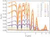Fig. 4 Scattered light albedo spectra Aλ(α) (Eq. (31)) as a function of wavelength at several viewing angles α, where α = 0° defines the sub-stellar point. Differences in the 3D cloud structure on the east and west hemispheres from the sub-stellar points produce small variations in Aλ across the 360° phase space at optical wavelengths. Na and K absorption are responsible for the drops in Aλ in the optical, while H2O features are the main absorber at near-IR to IR wavelengths.

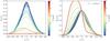Fig. 5 Left: scattered light phase curves of the albedo spectra Aλ(α) (Eq. (31)) of our HD 189733b simulation between 0.3 μm (colour bar: dark purple) to 5.0 μm (colour bar: dark red). Optical and near-IR wavelength packets are more strongly scattered than longer IR wavelengths. Right: classical phase function (Eq. (33)), which emphasises the phase curve shapes. Optical wavelengths are more symmetric about the sub-stellar point, IR wavelengths show more variation with phase. A Lambertian phase function (black, dashed line) is over-plotted for reference, which is useful for characterising scattering behaviour (see text).

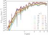Fig. 6 Emitted light spectral energy distribution λLp,em,λ (Eq. (37)) of our HD 189733b simulation as a function of wavelength at several viewing angles α (α = 0° is the sub-stellar point). Spectral features remain qualitatively similar at different viewing angles with a ~1 order of magnitude difference between the sub-stellar point (α = 0°) and anti-stellar point (α = −180°). The peak wavelength is found to be at ~2 μm.

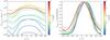Fig. 7 Left: emitted light spectral energy distribution λLp,em,λ (Eq. (37)) of our HD 189733b simulation phase curves between 0.3 μm (colour bar: dark purple) to 5.0 μm (colour bar: dark red). Infrared wavelengths from 3−5 μm dominate the emission luminosity at all phases. Right: normalised (to maximum λLp,em,λ) spectral energy distribution phase curves to emphasise the phase curve shapes. All wavelengths show a α≥ 10° eastward offset from the sub-stellar point.

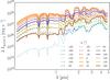Fig. 8 Combined scattered and emitted light spectral energy distribution λLp,tot,λ (Eq. (38)) of our HD 189733b simulation as a function of wavelength at several viewing angles α (α = 0° is the sub-stellar point). The optical wavelength scattered light luminosity drops off as the nightside of the planet is viewed. The emission features between the dayside and nightside are ~1 order of magnitude different dependent on wavelength.

We compare our classical phase function to the Lambertian phase function (Fig. 5, dashed black line), which is the phase function of a theoretical, perfectly isotropic scattering sphere (e.g. Seager 2010; Madhusudhan & Burrows 2012). This is useful for interpreting the type of scattering behaviour at east and west dayside hemispheres (Madhusudhan & Burrows 2012). The eastern hemisphere shows a classical phase function behaviour typical of Rayleigh-like scattering across all wavelengths, suggesting that the majority of optical and near-IR packets undergo a single scattering event in these regions. This region contains the smallest cloud particle sizes in the RHD simulation and lowest cloud opacity, increasing the likelihood of the packet escaping the boundaries without further interaction. The western hemisphere shows a mix of isotropic and Rayleigh-like scattering classical phase function behaviour for optical, near-IR and IR wavelengths. This suggests that packets experience multiple scattering events, which results in packets escaping in an isotropic manner. These regions contain some of the larger cloud particles on the dayside and an increased cloud scattering probability.

Figure 5 (right) also shows IR (3−5 μm) classical phase function asymmetry that arises from the differences in the opacity structure between the two day-night terminator regions. The westward limb (α = −90°) contains larger cloud particle sizes, opacity, and scattering probability in the IR compared to the eastern limb (α = 90°). The behaviour of the IR wavelength classical phase functions suggests that packets do not interact with the eastern terminator cloud structures and pass through without interaction, are absorbed, or interact with cloud particles on the nightside hemisphere since there is a return to the Lambertian function at nightside viewing angles. For the westward limb, the IR cloud opacity is higher, packets travel shallower into the atmosphere before interacting and are more likely to be scattered. These differences in cloud structures between the terminator regions result in a skewing of the IR classical phase function. The western side of the planet is therefore typically brighter in the IR by 10−20% in scattered light than the eastern side at comparable phases.

4.3. Emitted light spectra and phase curves

At secondary transit, observations are also sensitive to the thermal emission from the planetary atmosphere itself. Because the star-planet contrast is larger at IR wavelengths than in the optical, the planet’s atmospheric emission features are easier to detect.

Figure 6 shows the spectral energy distribution (SED) λL_p,emλ [erg s^-1] (Eq. (37)) as a function of wavelength for the atmospheric emitted light. We find that the SED follows similar trends across all viewing angles with ~1−2 mag differences between dayside and nightside emission luminosities. The peak of emission occurs at ~2 μm, where our model HD 189733b is brightest in emitted light. The least emission luminosity in the IR occurs at a viewing angle of α = −140°, corresponding to the coldest regions of the nightside.

Figure 7 (left) presents the planetary atmosphere SED λL_p,em,λ (Eq. (37)) as a function of viewing angle α. We find that emission is dominated by the longer IR wavelengths 2−5 μm for all phases. Emission at optical wavelengths is confined to the hottest dayside regions of the planet, however, this emission is >4 mag in luminosity smaller than IR wavelengths. A dip in luminosity is seen at ~−135°for all wavelengths, corresponding to the coldest nightside regions of the RHD simulation. Figure 7 (right) shows the normalised emitted light phase curves, which emphasises the shape of the phase curve. Most wavelengths show eastern offsets from the sub-stellar point in peak emission at 10−25°with some IR wavelengths showing offsets ~45° from the sub-stellar point.

We find that the effects of atmospheric scattering by emitted packets on the phase curves to be negligible. This is because of the low gas phase single scattering albedos (ω_gas< 10^-3) at IR wavelengths, which lowers the weights of the packets to negligible proportions after one or two scattering interactions. The majority of packets are then likely to be terminated by the Russian Roulette scheme, and those that survive will contain low luminosity weights in future interactions.

4.4. Total luminosities and observational predictions

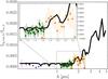Fig. 9 Combined scattered and emitted light flux ratio Lp,tot,λ/L⋆.λ of our HD 189733b simulation as a function of wavelength at secondary eclipse (α = 0°). We compare our HD 189733b simulation results to available observational data from HST STIS (purple dots, 0.29−0.57 μm; Evans et al. 2013), HST WFC3 (green diamonds, 1.13−1.64 μm; Crouzet et al. 2014), HST NICMOS (orange squares, 1.46−2.44 μm; Swain et al. 2009; Barstow et al. 2014), and Spitzer IRAC (magenta pentagons, 3.6 μm, 4.5 μm; Knutson et al. 2012).

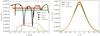Fig. 10 Combined scattered and emitted light flux ratio Lp,tot,λ/L⋆.λ HD 189733b predictions for the Kepler, TESS, and CHEOPS instruments. Left: predicted dayside flux ratio for Kepler (red dot), TESS (green square) and CHEOPS (orange diamond) photometric bandpasses. The solid black line is the model output. Dashed lines indicate the spectral response function of the instrument. Right: predicted Kepler (red), TESS (green) and CHEOPS (orange) flux ratio phase curves. All three instruments show no/little offset from the sub-stellar point, we predict a westward maximum flux offset of only −5°−0° from the sub-stellar point.

The observed luminosity from an exoplanet atmosphere is a combination of the reflected starlight and the emission from the planet itself. The component that dominates the observation will be wavelength- and phase-dependent owing to the 3D inhomogeneous scattering opacities (from cloud particles) and temperature profiles (from atmospheric circulation) of the planet. Such inhomogeneity is present in the results of the HD 189733b RHD cloud forming simulation. In this section, we combine our scattering and thermal emission results above to produce observable quantities in the TESS (Ricker et al. 2014) and CHEOPS (Broeg et al. 2013) bandpasses for our HD 189733b model. We also compare to readily available observational data from current/past missions. We also produce Kepler band predictions, despite K2 not scheduled to observe HD 189733b to allow a comparison to other studies focused on modelling Kepler objects (e.g. Parmentier et al. 2016).

The total monochromatic luminosity from the planet is the sum of the reflected light and emitted light 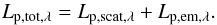${\mathit{L}}_{\mathrm{p}\mathit{,}\mathrm{tot}\mathit{,\lambda }}\mathrm{=}{\mathit{L}}_{\mathrm{p}\mathit{,}\mathrm{scat}\mathit{,\lambda }}\mathrm{+}{\mathit{L}}_{\mathrm{p}\mathit{,}\mathrm{em}\mathit{,\lambda }}\mathit{.}$(38)The apparent geometric albedo (which includes scattered and emitted light) is then 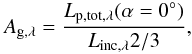${\mathit{A}}_{\mathrm{g}\mathit{,\lambda }}\mathrm{=}\frac{{\mathit{L}}_{\mathrm{p}\mathit{,}\mathrm{tot}\mathit{,\lambda }}\mathrm{(}\mathit{\alpha }\mathrm{=}\mathrm{0}°\mathrm{)}}{{\mathit{L}}_{\mathrm{inc}\mathit{,\lambda }}\mathrm{2}\mathit{/}\mathrm{3}}\mathit{,}$(39)in which the numerator and denominator are integrated across the Kepler, TESS, and CHEOPS bandpasses. For our comparisons to observational data and observational predictions, instead of assuming the host star radiates as a black body in previous sections, the stellar monochromatic luminosity of HD 189733 (L_⋆,λ) is taken from the Kurucz¹ stellar atmosphere model for HD 189733.

Figure 8 shows the spectral luminosity of the planet as a function of phase including both the scattering and emitted components. On the dayside of the planet, the luminosity from scattered light is at a similar magnitude to the IR emission. For nightside profiles, the scattered light fraction drops off and the emitted luminosity dominates.

Figure 9 presents the flux ratio L_p,tot,λ/L_⋆,λ of our combined scattered and emitted light, compared to the HST secondary eclipse data from Swain et al. (2009), Evans et al. (2013), Crouzet et al. (2014), Barstow et al. (2014) and Spitzer data from Knutson et al. (2012). Similar to Sect. 4.1, our simulation is consistent with the B band HST STIS data from Evans et al. (2013) but overestimates the planet-star flux ratio for the V band. The results are consistent with the HST WFC3 (Crouzet et al. 2014) and NICMOS (Swain et al. 2009; Barstow et al. 2014) spectral trends, with offsets in the amplitude of these features. Several retrieval models on this and similar observational data (e.g. Madhusudhan & Seager 2009; Lee et al. 2012; Line et al. 2012, 2014) suggest a possible sub-solar H₂O abundance on the dayside of HD 189733b, which would lower the amplitude of the H₂O features in our results. Our results are also consistent with the 3.6 μm and 4.5 μm Spitzer IRAC photometry observations of Knutson et al. (2012). Overall, our current model reproduces the secondary transit optical to near-IR observational trends well.

Figure 10 (left) shows the dayside flux ratio predictions for Kepler, TESS, and CHEOPS bandpasses. We predict a ~10% difference in peak flux ratio between the CHEOPS and TESS bandpasses. This is directly due to the sensitivity of the CHEOPS bandpass to the optical scattering component of our RHD modelled cloud particles, while the TESS bandpass is unaffected by this component and more sensitive to the near-IR thermal emission of the HD 189733b model.

Figure 10 (right) presents the flux ratio phase curves for the Kepler, TESS, and CHEOPS bandpasses. Our modelling results show that we expect HD 189733b to have a zero or small westward offset of no less than −5° from the sub-stellar point for the Kepler, TESS, and CHEOPS bands. This suggests that the cloud particle differences (size, composition, etc.) at the east and western hemispheres in our RHD simulation are not radically different enough to produce the larger (<−10°) westward offsets seen for some Kepler planets. The TESS and CHEOPS photometry become comparable at greater longitudes as the cloud particle scattering component becomes less dominant compared to the thermal emission (Fig. 8).

If the extra absorption component from the Evans et al. (2013) HST STIS measurements at ~0.4−0.5 μm is taken into account, owing to the bandpass efficiencies, the Kepler and CHEOPS contrast ratios and geometric albedos of HD 189733b are likely to be lower than those presented here. However, the TESS photometric band would be relatively unaffected owing to the low sensitivity in this wavelength regime, unless the influence of this absorber extends into the near-IR. Table 2 summarises our Kepler, TESS, and CHEOPS predictions, including estimates of the geometric albedo A_g (Eq. (39)) in each respective band.

4.5. Variance and convergence

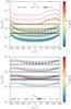Fig. 11 Scattered light (top) and emitted light (bottom), noise error σ (Eq. (40)) with viewing angle α and wavelength (colour bar). The nominal noise error values for Ninc/atm = 105 (dash-dot line), 106 (dashed line), 107 (solid line) and 108 (dotted line) are the horizontal black lines. Most scattered and emitted light images are near or below the nominal values, suggesting that each packet contributes once or more to multiple images.

We conclude the results section with a discussion on the noise errors and convergence of the MCRT results. Because of the stochastic nature of MCRT, it exhibits Poisson sampling statistics, where the noise error σ is given by $\mathit{\sigma }\mathrm{=}\frac{\mathrm{1}}{\sqrt{{\mathit{N}}_{\mathrm{im}}}}\mathit{,}$(40)where N_im(λ, α) is the number of photon packets contributing to the output image, dependent on the wavelength and viewing angle. To test the convergence of the results, the same experiments are performed with a varying number of initialised photon packets. We repeat the above simulations with N_inc/atm = 10⁵, 10⁶ and 10⁷ to test the decrease of σ with initialised packet numbers.

Figure 11 shows the noise error of each scattered and emitted light image for our three N_inc/atm simulations with viewing angle α and wavelength. We also show the nominal value (black horizontal line) from the total initialised photons (N_inc, N_atm). In incident scattered light, all but the longest IR wavelengths show noise errors below the nominal values, indicating that most incident stellar packets contribute to one or more image results. In thermal emitted light, the noise error values are within 2−3 times the nominal value, suggesting that most thermally emitted photons also contribute to many image outputs. The error only increases by a factor of 2 or 3 for images including a nightside component, which suggests that composite emission biasing was successful in more evenly spreading the noise error between high and low luminosity regions. Our presented results of the previous sections using N_inc = 10⁷, N_atm = 10⁸, have a typical model noise error of <0.1%.

5. Discussion

In this section we discuss the overall context of our results both theoretically and observationally, and detail some of the limitations of the current simulations. In summary, our updated model improves the realism of the Hood et al. (2008) scheme in several ways:

• cloud particle opacity and scattering properties, derived from 3Dself-consistent cloud forming RHD simulation results;

• addition of a thermal emission mode, using the thermodynamic properties of the 3D RHD simulation results;

• higher radial, longitude, latitude resolution (R, φ, θ) = (100, 160, 64) given by the RHD grid cell sizes;

• k-distribution opaque absorbing gas species to the opacity scheme interpolated to the 3D RHD T-p profiles;

• addition of survival biasing and composite biasing variance reduction techniques for the MCRT scheme;

• stochastic cloud particle size distribution sampling, based on the microphysical cloud formation results of the RHD simulation;

• Rayleigh scattering for small cloud particle size parameters and H₂ molecular scattering;

• two-term Henyey-Greenstein scattering for larger size parameter cloud particle scattering events.

In Hood et al. (2008) a fractal scheme was introduced to their simplified cloudy atmosphere structure to model “patchiness” in small scale cloud properties. These authors found that increasing the porosity of their original smoothly distributed cloud structure decreased the geometric albedo results, as L-packets passed more easily through cloudy regions to the deeper atmosphere. Applying a similar technique to the current study may reconcile the differences in geometric albedo of the model to the observational data. We note that the amount of porosity is not known a priori, however.

Our current study depends on the 3D cloud forming HD 189733b RHD model results of Lee et al. (2016). We summarise the limitations of that study and the possible effects on the MCRT results presented here. The long-term (1000 s simulated days) settling timescales of the sub-micron cloud particles in the upper atmosphere is not captured by our ~60 Earth days of total integration (e.g. Woitke & Helling 2003; Parmentier et al. 2013). The possible removal of sub-micron grains from the upper atmosphere would have two main effects: lowering the overall opacity of the upper atmospheric cloud and increasing the likelihood of cloud particle Rayleigh scattering events as the size distribution is further skewed towards smaller particle sizes. However, sub-micron grains are likely to remain lofted over long timescale in the atmospheres of hot Jupiters from hydrodynamical motions alone (Parmentier et al. 2013), suggesting that a total rain out of sub-micron cloud particles is an unlikely scenario.

Our gas phase opacities in Paper I used Planck mean opacities, which have been shown to have band averaged errors for the stellar heating rates (Amundsen et al. 2014). This may be offset by the greyer opacity of the cloud particles, but regions where the gas opacity dominates (e.g. high-temperature dayside regions) these errors may remain. Although in this post-processing study we use k-distribution tables, the cloud properties derived from the RHD model may be affected by this choice of opacity scheme. We suggest in Lee et al. (2016) that the use of the correlated-k approximation would alter the depth of the seed particle regions on the dayside of the RHD model, dependent on whether the dayside atmosphere is cooler or warmer because of this opacity change. This would alter the cloud opacity structure; the effect on the MCRT would most likely be an increased or decreased luminosity escaping from the next-event estimator scheme, depending on whether the main scattering regions were higher or lower in atmospheric optical depth. Additionally, the Lee et al. (2016) simulation assumed an absorptive opacity, neglecting scattering effects of clouds particles, which would also impact the thermal structure of the RHD results.

Fe[s] materials were also not modelled in Lee et al. (2016), which may also increase the opacity of cloud particles and reduce the single-scattering albedo of cloud particles owing to the absorbing properties of Fe[s] materials. However, Fe[s] rich grains are expected to reside below the photosphere of HD 189733b (Lee et al. 2015; Helling et al. 2016a), where they would have negligible effects on the observable scattered and emitted light.

Our model does not reproduce the low V band geometric albedo observed by Evans et al. (2013). This low geometric albedo has been noted by other studies (e.g. Barstow et al. 2014), with a suggestion that another, unknown absorber is responsible for the sharp decrease in albedo at 0.5 μm. Barstow et al. (2014) modelled several scenarios that could be responsible for this decrease: super-solar Na abundance, which would extend the Na absorption wings; TiO absorption; and also MnS[s] cloud compositions. If the effects of this unknown absorber extend into the near-IR wavelength regime, we can expect a lower geometric albedo for the TESS and CHEOPS bandpasses than the chemical equilibrium, solar-metallicity gas opacity calculations applied here.

Our CHEOPS and TESS predictions show that we predict the CHEOPS band to be brighter by ~10% than the TESS photometric band, largely because CHEOPS is sensitive to optical wavelength scattering due to cloud particles at wavelengths 0.33−0.50 μm. We suggest that by comparing CHEOPS and TESS geometric albedos, qualitative information about the cloud particles of an exoplanet can be derived. A similar suggestion was stated by Placek et al. (2016) which modelled disentangling scattered and emitted components from a combined Kepler and TESS photometry for revisited Kepler field planets. If the CHEOPS band is brighter than the TESS bandpass, our modelling suggests that an optical wavelength scattering cloud particle is present. While if the TESS band is brighter or nearer in brightness to the CHEOPS band, this is suggestive of a cloud-free or less/patchy cloudy planet since TESS is more sensitive to the near-IR thermal emission from an atmosphere than CHEOPS. If different offsets in maximum flux in phase curves between the CHEOPS and TESS bands are present, this suggests a patchy cloud scenario, where CHEOPS is periodically more sensitive to optical wavelength scattering by clouds confined to one hemisphere of the planet compared to TESS. We note that additional evidence (e.g. transit spectroscopy) is required to more conclusively infer cloud particle information. However, this information may help identify planet candidates for more detailed spectrometer follow-up observations where observation time is more limited.

Our model generally supports the conclusions of Parmentier et al. (2016) which, in their GCM model grids, show that planets at the effective temperature of HD 189733b (T_eq~ 1200 K) would be bright in the Kepler band owing to the scattered light from cloud particles. Our model agrees well with their non-cold trapped 0.1 μm particle Kepler band A_g~ 0.20 scenario, but is less consistent with the 0.1 μm particle cold trap scenario, where A_g~ 0.45. Our model is also reasonably consistent with their 1.0 μm particle size scenarios, where A_g~ 0.25−0.30. We are also able to reproduce their prediction of a zero/small westward offset in the Kepler band for the T_eq = 1200 K model for all particle size and cold trap scenarios. However, they suggest that MnS[s] and Na₂S[s] cloud materials may be more dominant than a silicate cloud (modelled here) for HD 189733b, possibly leading to different scattered light behaviour and variations in geometric albedo than those presented here. Na₂S[s] condensation may also alter the gas phase Na abundance between the planet limbs and the dayside (where Na₂S[s] is likely to evaporate), which would affect the albedo spectra.

6. Summary and conclusions

In this investigation we have examined the scattering and emission properties of our HD 189733b 3D cloud forming RHD simulation from Paper I. We developed a Monte Carlo radiative transfer forward model for post-processing of atmospheric GCM/RHD output to produce combined scattered and emitted light observables. We have shown that the wavelength-dependent 3D inhomogeneous cloud opacity and scattering behaviour of cloud particles can produce differences in phase curve behaviour between the east and west hemispheres of the planet. Our combined scattered and emitted light simulations are consistent with available HST and Spitzer observations, with deviations most likely occurring because of due to a decreased H₂O abundance from solar (e.g. Crouzet et al. 2014) and an unknown extra absorber at ~0.5 μm (Evans et al. 2013; Barstow et al. 2014). We also predict that the CHEOPS bandpass will be ~10% brighter than the TESS bandpass, because of the sensitivity of CHEOPS to optical wavelength scattering compared to TESS. We suggest that qualitative information about the nature of the cloud particles on exoplanets can be inferred by comparing the relative geometric albedos and phase curve offsets of TESS and CHEOPS photometry data. However, we emphasise the importance of obtaining high quality spectroscopic data in quantitatively inferring the cloud properties and atmospheric composition of exoplanet atmospheres. Specific conclusions of our HD 189733b model results include

• A strong Rayleigh and/or backscattering Mie scatteringcomponent is likely required to increase the geometric albedo toobserved levels in the HST B band STIS measurements.

• We find that the eastern hemisphere of our HD 189733b model is more dominated by single scattering events, resulting in a Rayleigh-like classical phase function, while the western hemisphere is likely to have multiple-scattering events, resulting in a more isotropic classical phase function.

• Combined scattered and emitted light SEDs show that our model HD 189733b planet is likely to be at a similar brightness across 0.3−5 μm on the dayside of the planet.

• IR wavelengths can show westward offsets in scattered light phase curves. However, in this case, the overall magnitude of light scattered at these wavelengths is low.

• We suggest HD 189733b to have apparent geometric albedos A_g~ 0.222, 0.205, and 0.229 in the Kepler, TESS, and CHEOPS photometric bands, respectively.

• We suggest HD 189733b may exhibit a zero or small (~−5°) westward offset in the TESS and CHEOPS photometric bands.

The Monte Carlo radiative-transfer model framework presented here can be further extended to model other observable properties, such as transmission spectra, and other photon microphysical processes, such as photochemical haze formation. Three-dimensional observables of 1D atmospheric models may also be readily simulated using this MCRT framework.

Acknowledgments

We thank the anonymous referee for constructive and insightful suggestions, which improved the manuscript and MCRT model substantially. E.L. and Ch.H. highlight the financial support of the European community under the FP7 ERC starting grant 257431. Our local HPC computational support at Abu Dhabi and St Andrews is highly acknowledged. We thank A. Collier-Cameron and D. Futyan for help with CHEOPS bandpass data. We thank A. Mortier, K. Hay, and current/former members of the LEAP team for insightful discussions and suggestions. Most plots were produced using the community open-source Python packages Matplotlib, SciPy, and AstroPy.

References

All Tables

All Figures

Fig. 1 Incident scattered (left) and atmospheric emitted (right) light image array of the L-packet luminosity fractions fx,y(λ,α) ∈ (0, 1) escaping from the HD 189733b simulation. These images are produced by the next event estimator method at 1.0 μm for a viewing angle/phase of α = 60° (eastern dayside). The sharp transition from blue to black at pixel numbers x = 120−150 is the eastern terminator in the scattered light image, including a “twilight” effect where packets scatter past the terminator line. The effect of the grid structure on the images is more apparent in the emitted light, since packets are initialised from within the cell volumes.

In the text

	Fig. 2 Diagram visualising the definition of equatorial viewing angle α [°] used in this study. Viewing angles east of the sub-stellar point are positively defined, while regions west of the sub-stellar point are negatively defined.
In the text

Fig. 3 Scattered light apparent geometric albedo Ag,λ (Eq. (32)) of our HD 189733b simulation output compared to Evans et al. (2013)’s individual HST STIS measurements. The total contribution is indicated by the solid blue line; TTHG cloud particle scattering by the dashed orange line; Rayleigh cloud particle scattering by the teal dash-dotted line; H2 Rayleigh scattering by the brown solid line. Left (0.29−0.6 μm): the Rayleigh and TTHG model is generally consistent with the B band HST STIS measurements, but does not predict the low albedo of the V band. Right (0.29−5 μm): extended spectra from 0.3−5 μm, showing the convolved B band and V band measurements from Evans et al. (2013). Ag,λ becomes negligible beyond 5 μm.

In the text

Fig. 4 Scattered light albedo spectra Aλ(α) (Eq. (31)) as a function of wavelength at several viewing angles α, where α = 0° defines the sub-stellar point. Differences in the 3D cloud structure on the east and west hemispheres from the sub-stellar points produce small variations in Aλ across the 360° phase space at optical wavelengths. Na and K absorption are responsible for the drops in Aλ in the optical, while H2O features are the main absorber at near-IR to IR wavelengths.

In the text

Fig. 5 Left: scattered light phase curves of the albedo spectra Aλ(α) (Eq. (31)) of our HD 189733b simulation between 0.3 μm (colour bar: dark purple) to 5.0 μm (colour bar: dark red). Optical and near-IR wavelength packets are more strongly scattered than longer IR wavelengths. Right: classical phase function (Eq. (33)), which emphasises the phase curve shapes. Optical wavelengths are more symmetric about the sub-stellar point, IR wavelengths show more variation with phase. A Lambertian phase function (black, dashed line) is over-plotted for reference, which is useful for characterising scattering behaviour (see text).

In the text

Fig. 6 Emitted light spectral energy distribution λLp,em,λ (Eq. (37)) of our HD 189733b simulation as a function of wavelength at several viewing angles α (α = 0° is the sub-stellar point). Spectral features remain qualitatively similar at different viewing angles with a ~1 order of magnitude difference between the sub-stellar point (α = 0°) and anti-stellar point (α = −180°). The peak wavelength is found to be at ~2 μm.

In the text

Fig. 7 Left: emitted light spectral energy distribution λLp,em,λ (Eq. (37)) of our HD 189733b simulation phase curves between 0.3 μm (colour bar: dark purple) to 5.0 μm (colour bar: dark red). Infrared wavelengths from 3−5 μm dominate the emission luminosity at all phases. Right: normalised (to maximum λLp,em,λ) spectral energy distribution phase curves to emphasise the phase curve shapes. All wavelengths show a α≥ 10° eastward offset from the sub-stellar point.

In the text

Fig. 8 Combined scattered and emitted light spectral energy distribution λLp,tot,λ (Eq. (38)) of our HD 189733b simulation as a function of wavelength at several viewing angles α (α = 0° is the sub-stellar point). The optical wavelength scattered light luminosity drops off as the nightside of the planet is viewed. The emission features between the dayside and nightside are ~1 order of magnitude different dependent on wavelength.

In the text

Fig. 9 Combined scattered and emitted light flux ratio Lp,tot,λ/L⋆.λ of our HD 189733b simulation as a function of wavelength at secondary eclipse (α = 0°). We compare our HD 189733b simulation results to available observational data from HST STIS (purple dots, 0.29−0.57 μm; Evans et al. 2013), HST WFC3 (green diamonds, 1.13−1.64 μm; Crouzet et al. 2014), HST NICMOS (orange squares, 1.46−2.44 μm; Swain et al. 2009; Barstow et al. 2014), and Spitzer IRAC (magenta pentagons, 3.6 μm, 4.5 μm; Knutson et al. 2012).

In the text

Fig. 10 Combined scattered and emitted light flux ratio Lp,tot,λ/L⋆.λ HD 189733b predictions for the Kepler, TESS, and CHEOPS instruments. Left: predicted dayside flux ratio for Kepler (red dot), TESS (green square) and CHEOPS (orange diamond) photometric bandpasses. The solid black line is the model output. Dashed lines indicate the spectral response function of the instrument. Right: predicted Kepler (red), TESS (green) and CHEOPS (orange) flux ratio phase curves. All three instruments show no/little offset from the sub-stellar point, we predict a westward maximum flux offset of only −5°−0° from the sub-stellar point.

In the text

Fig. 11 Scattered light (top) and emitted light (bottom), noise error σ (Eq. (40)) with viewing angle α and wavelength (colour bar). The nominal noise error values for Ninc/atm = 105 (dash-dot line), 106 (dashed line), 107 (solid line) and 108 (dotted line) are the horizontal black lines. Most scattered and emitted light images are near or below the nominal values, suggesting that each packet contributes once or more to multiple images.

In the text

References

- Ackerman, A. S., & Marley, M. S. 2001, ApJ, 556, 872 [Google Scholar]
- Agol, E., Cowan, N. B., Knutson, H. A., et al. 2010, ApJ, 721, 1861 [Google Scholar]
- Amundsen, D. S., Baraffe, I., Tremblin, P., et al. 2014, A&A, 564, A59 [NASA ADS] [CrossRef] [EDP Sciences] [Google Scholar]
- Amundsen, D. S., Mayne, N. J., Baraffe, I., et al. 2016, A&A, 595, A36 [NASA ADS] [CrossRef] [EDP Sciences] [Google Scholar]
- Angerhausen, D., DeLarme, E., & Morse, J. A. 2015, PASP, 127, 1113 [NASA ADS] [CrossRef] [Google Scholar]
- Baes, M., Gordon, K. D., Lunttila, T., et al. 2016, A&A, 590, A55 [NASA ADS] [CrossRef] [EDP Sciences] [Google Scholar]
- Barstow, J. K., Aigrain, S., Irwin, P. G. J., et al. 2014, ApJ, 786, 154 [NASA ADS] [CrossRef] [Google Scholar]
- Broeg, C., Fortier, A., Ehrenreich, D., et al. 2013, in EPJ Web Conf., 47, 03005 [Google Scholar]
- Cahoy, K. L., Marley, M. S., & Fortney, J. J. 2010, ApJ, 724, 189 [Google Scholar]
- Charbonneau, D., Knutson, H. A., Barman, T., et al. 2008, ApJ, 686, 1341 [NASA ADS] [CrossRef] [Google Scholar]
- Crouzet, N., McCullough, P. R., Deming, D., & Madhusudhan, N. 2014, ApJ, 795, 166 [NASA ADS] [CrossRef] [Google Scholar]
- Dalgarno, A., & Williams, D. A. 1962, ApJ, 136, 690 [NASA ADS] [CrossRef] [Google Scholar]
- de Kok, R. J., & Stam, D. M. 2012, Icarus, 221, 517 [CrossRef] [Google Scholar]
- Demory, B.-O., de Wit, J., Lewis, N., et al. 2013, ApJ, 776, L25 [Google Scholar]
- Dobbs-Dixon, I., & Agol, E. 2013, MNRAS, 435, 3159 [NASA ADS] [CrossRef] [Google Scholar]
- Draine, B. T. 2003, ApJ, 598, 1017 [NASA ADS] [CrossRef] [Google Scholar]
- Dupree, S. A., & Fraley, S. K. 2002, A Monte Carlo Primer (New York: Kluwer Academic/Plenum Publishers) [Google Scholar]
- Dyudina, U., Zhang, X., Li, L., et al. 2016, ApJ, 822, 76 [Google Scholar]
- Esteves, L. J., De Mooij, E. J. W., & Jayawardhana, R. 2015, ApJ, 804, 150 [Google Scholar]
- Evans, T. M., Pont, F., Sing, D. K., et al. 2013, ApJ, 772, L16 [NASA ADS] [CrossRef] [Google Scholar]
- Fortney, J. J., Cooper, C. S., Showman, A. P., Marley, M. S., & Freedman, R. S. 2006, ApJ, 652, 746 [CrossRef] [Google Scholar]
- Garcia Munoz, A., & Isaak, K. G. 2015, Proceedings of the National Academy of Science, 112, 13461 [NASA ADS] [CrossRef] [Google Scholar]
- Goody, R., West, R., Chen, L., & Crisp, D. 1989, J. Quant. Spec. Radiat. Transf., 42, 539 [NASA ADS] [CrossRef] [Google Scholar]
- Grimm, S. L., & Heng, K. 2015, ApJ, 808, 182 [NASA ADS] [CrossRef] [Google Scholar]
- Hansen, J. E., & Travis, L. D. 1974, Space Sci. Rev., 16, 527 [Google Scholar]
- Harries, T. J., Monnier, J. D., Symington, N. H., & Kurosawa, R. 2004, MNRAS, 350, 565 [NASA ADS] [CrossRef] [Google Scholar]
- Heintzenberg, J. 1994, Aerosol Science and Technology, 21, 46 [NASA ADS] [CrossRef] [Google Scholar]
- Helling, C., Lee, G., Dobbs-Dixon, I., et al. 2016a, MNRAS, 460, 855 [NASA ADS] [CrossRef] [Google Scholar]
- Helling, C., Rimmer, P. B., Rodriguez-Barrera, I. M., et al. 2016b, Plasma Physics and Controlled Fusion, 58, 074003 [NASA ADS] [CrossRef] [Google Scholar]
- Heng, K., & Demory, B.-O. 2013, ApJ, 777, 100 [NASA ADS] [CrossRef] [Google Scholar]
- Henyey, L. G., & Greenstein, J. L. 1941, ApJ, 93, 70 [Google Scholar]
- Hood, B., Wood, K., Seager, S., & Collier Cameron, A. 2008, MNRAS, 389, 257 [NASA ADS] [CrossRef] [Google Scholar]
- Kataria, T., Sing, D. K., Lewis, N. K., et al. 2016, ApJ, 821, 9 [NASA ADS] [CrossRef] [Google Scholar]
- Kattawar, G. W. 1975, J. Quant. Spec. Radiat. Transf., 15, 839 [NASA ADS] [CrossRef] [Google Scholar]
- Knutson, H. A., Charbonneau, D., Allen, L. E., et al. 2007, Nature, 447, 183 [NASA ADS] [CrossRef] [Google Scholar]
- Knutson, H. A., Charbonneau, D., Cowan, N. B., et al. 2009, ApJ, 690, 822 [NASA ADS] [CrossRef] [Google Scholar]
- Knutson, H. A., Lewis, N., Fortney, J. J., et al. 2012, ApJ, 754, 22 [NASA ADS] [CrossRef] [Google Scholar]
- Kopparla, P., Natraj, V., Zhang, X., et al. 2016, ApJ, 817, 32 [NASA ADS] [CrossRef] [Google Scholar]
- Kreidberg, L., Bean, J. L., Désert, J.-M., et al. 2014, Nature, 505, 69 [Google Scholar]
- Lacis, A. A., & Oinas, V. 1991, J. Geophys. Res., 96, 9027 [Google Scholar]
- Lee, G., Helling, C., Dobbs-Dixon, I., & Juncher, D. 2015, A&A, 580, A12 [NASA ADS] [CrossRef] [EDP Sciences] [Google Scholar]
- Lee, G., Dobbs-Dixon, I., Helling, C., Bognar, K., & Woitke, P. 2016, A&A, 594, A48 [NASA ADS] [CrossRef] [EDP Sciences] [Google Scholar]
- Lee, J.-M., Fletcher, L. N., & Irwin, P. G. J. 2012, MNRAS, 420, 170 [NASA ADS] [CrossRef] [Google Scholar]
- Line, M. R., Zhang, X., Vasisht, G., et al. 2012, ApJ, 749, 93 [Google Scholar]
- Line, M. R., Knutson, H., Wolf, A. S., & Yung, Y. L. 2014, ApJ, 783, 70 [Google Scholar]
- Lucy, L. B. 1999, A&A, 344, 282 [NASA ADS] [Google Scholar]
- Madhusudhan, N., & Burrows, A. 2012, ApJ, 747, 25 [NASA ADS] [CrossRef] [Google Scholar]
- Madhusudhan, N., & Seager, S. 2009, ApJ, 707, 24 [NASA ADS] [CrossRef] [Google Scholar]
- Marley, M. S., & McKay, C. P. 1999, Icarus, 138, 268 [NASA ADS] [CrossRef] [Google Scholar]
- Marley, M. S., Gelino, C., Stephens, D., Lunine, J. I., & Freedman, R. 1999, ApJ, 513, 879 [NASA ADS] [CrossRef] [Google Scholar]
- Mayer, B. 2009, in EPJ Web Conf., 1, 75 [Google Scholar]
- Min, M., Dullemond, C. P., Dominik, C., de Koter, A., & Hovenier, J. W. 2009, A&A, 497, 155 [NASA ADS] [CrossRef] [EDP Sciences] [Google Scholar]
- Morley, C. V., Fortney, J. J., Marley, M. S., et al. 2015, ApJ, 815, 110 [NASA ADS] [CrossRef] [Google Scholar]
- Oreshenko, M., Heng, K., & Demory, B.-O. 2016, MNRAS, 457, 3420 [NASA ADS] [CrossRef] [Google Scholar]
- Parmentier, V., Showman, A. P., & Lian, Y. 2013, A&A, 558, A91 [NASA ADS] [CrossRef] [EDP Sciences] [Google Scholar]
- Parmentier, V., Fortney, J. J., Showman, A. P., Morley, C., & Marley, M. S. 2016, ApJ, 828, 22 [Google Scholar]
- Perez-Becker, D., & Showman, A. P. 2013, ApJ, 776, 134 [NASA ADS] [CrossRef] [Google Scholar]
- Pfeiffer, N., & Chapman, G. H. 2008, Optics Express, 16, 13637 [NASA ADS] [CrossRef] [Google Scholar]
- Pinte, C., Ménard, F., Duchêne, G., & Bastien, P. 2006, A&A, 459, 797 [NASA ADS] [CrossRef] [EDP Sciences] [Google Scholar]
- Placek, B., Knuth, K. H., & Angerhausen, D. 2016, PASP, 128, 074503 [NASA ADS] [CrossRef] [Google Scholar]
- Ricker, G. R., Winn, J. N., Vanderspek, R., et al. 2014, in Space Telescopes and Instrumentation 2014: Optical, Infrared, and Millimeter Wave, Proc. SPIE, 9143, 914320 [NASA ADS] [CrossRef] [Google Scholar]
- Rijkhorst, E.-J., Plewa, T., Dubey, A., & Mellema, G. 2006, A&A, 452, 907 [NASA ADS] [CrossRef] [EDP Sciences] [Google Scholar]
- Rimmer, P. B., & Helling, C. 2016, ApJS, 224, 9 [NASA ADS] [CrossRef] [Google Scholar]
- Robitaille, T. P. 2011, A&A, 536, A79 [NASA ADS] [CrossRef] [EDP Sciences] [Google Scholar]
- Seager, S. 2010, Exoplanet Atmospheres: Physical Processes (Princeton University Press) [Google Scholar]
- Seager, S., Whitney, B. A., & Sasselov, D. D. 2000, ApJ, 540, 504 [NASA ADS] [CrossRef] [Google Scholar]
- Sharp, C. M., & Burrows, A. 2007, ApJS, 168, 140 [NASA ADS] [CrossRef] [Google Scholar]
- Showman, A. P., Fortney, J. J., Lian, Y., et al. 2009, ApJ, 699, 564 [NASA ADS] [CrossRef] [Google Scholar]
- Shporer, A., & Hu, R. 2015, AJ, 150, 112 [NASA ADS] [CrossRef] [Google Scholar]
- Stap, F. A., Hasekamp, O. P., Emde, C., & Röckmann, T. 2016, J. Quant. Spectr. Rad. Transf., 170, 54 [NASA ADS] [CrossRef] [Google Scholar]
- Stark, C. R., Helling, C., & Diver, D. A. 2015, A&A, 579, A41 [NASA ADS] [CrossRef] [EDP Sciences] [Google Scholar]
- Steinacker, J., Baes, M., & Gordon, K. D. 2013, ARA&A, 51, 63 [CrossRef] [Google Scholar]
- Swain, M. R., Vasisht, G., Tinetti, G., et al. 2009, ApJ, 690, L114 [CrossRef] [Google Scholar]
- Toon, O. B., McKay, C. P., Ackerman, T. P., & Santhanam, K. 1989, J. Geophys. Res., 94, 16287 [Google Scholar]
- Torres, G., Winn, J. N., & Holman, M. J. 2008, ApJ, 677, 1324 [Google Scholar]
- Watkins, C., & Cho, J. Y.-K. 2010, ApJ, 714, 904 [NASA ADS] [CrossRef] [Google Scholar]
- Webber, M. W., Lewis, N. K., Marley, M., et al. 2015, ApJ, 804, 94 [NASA ADS] [CrossRef] [Google Scholar]
- Whitney, B. A. 2011, Bulletin of the Astronomical Society of India, 39, 101 [NASA ADS] [Google Scholar]
- Whitney, B. A., Wood, K., Bjorkman, J. E., & Wolff, M. J. 2003, ApJ, 591, 1049 [Google Scholar]
- Wiktorowicz, S. J., Nofi, L. A., Jontof-Hutter, D., et al. 2015, ApJ, 813, 48 [NASA ADS] [CrossRef] [Google Scholar]
- Woitke, P., & Helling, C. 2003, A&A, 399, 297 [NASA ADS] [CrossRef] [EDP Sciences] [Google Scholar]
- Woitke, P., & Helling, C. 2004, A&A, 414, 335 [NASA ADS] [CrossRef] [EDP Sciences] [Google Scholar]
- Wolf, S., & Voshchinnikov, N. V. 2004, Comput. Phys. Commun., 162, 113 [Google Scholar]
- Wood, K., & Loeb, A. 2000, ApJ, 545, 86 [NASA ADS] [CrossRef] [Google Scholar]
- Wood, K., & Reynolds, R. J. 1999, ApJ, 525, 799 [NASA ADS] [CrossRef] [Google Scholar]
- Yusef-Zadeh, F., Morris, M., & White, R. L. 1984, ApJ, 278, 186 [CrossRef] [Google Scholar]
- Zender, C. 2015, Particle size distributions: Theory and application aerosols, clouds, and soils, http://dust.ess.uci.edu/facts/psd/psd.pdf [Google Scholar]
All Tables
HD 189733 system parameters adopted for this study. We use the parameters presented in Torres et al. (2008).