| Issue |
A&A
Volume 600, April 2017
|
|
|---|---|---|
| Article Number | A81 | |
| Number of page(s) | 82 | |
| Section | Stellar structure and evolution | |
| DOI | https://doi.org/10.1051/0004-6361/201628914 | |
| Published online | 04 April 2017 | |
The VLT-FLAMES Tarantula Survey
XXIV. Stellar properties of the O-type giants and supergiants in 30 Doradus ⋆,⋆⋆
1 Astronomical Institute Anton Pannekoek, Amsterdam University, Science Park 904, 1098 Amsterdam, The Netherlands
e-mail: This email address is being protected from spambots. You need JavaScript enabled to view it.
2 Argelander-Institut für Astronomie, Universität Bonn, Auf dem Hügel 71, 53121 Bonn, Germany
3 UK Astronomy Technology Centre, Royal Observatory Edinburgh, Blackford Hill, Edinburgh, EH9 3HJ, UK
4 Institute of Astrophysics, KU Leuven, Celestijnenlaan 200D, 3001 Leuven, Belgium
5 European Space Astronomy Centre (ESAC), Camino bajo del Castillo, s/n Urbanizacion Villafranca del Castillo, Villanueva de la Cañada, 28 692 Madrid, Spain
6 Department of Physics, University of Oxford, Keble Road, Oxford OX1 3RH, UK
7 LMU Munich, Universitätssternwarte, Scheinerstrasse 1, 81679 München, Germany
8 Institute of Astronomy with NAO, Bulgarian Academy of Sciences, PO Box 136, 4700 Smoljan, Bulgaria
9 Max-Planck-Institut für Astronomie, Königstuhl 17, 69117 Heidelberg, Germany
10 Department of Astronomy, University of Michigan, 1085 S. University Avenue, Ann Arbor, MI 48109-1107, USA
11 Department of Physics & Astronomy, University of Sheffield, Hounsfield Road, Sheffield, S3 7RH, UK
12 Centro de Astrobiología (CSIC-INTA), Ctra. de Torrejón a Ajalvir km-4, 28850 Torrejón de Ardoz, Madrid, Spain
13 Departamento de Astrofísica, Universidad de La Laguna, Avda. Astrofísico Francisco Sánchez s/n, 38071 La Laguna, Tenerife, Spain
14 Instituto de Astrofísica de Canarias, C/Vía Láctea s/n, 38200 La Laguna, Tenerife, Spain
15 Centro de Astrobiología (CSIC-INTA), ESAC campus, Camino bajo del castillo s/n, Villanueva de la Cañada, 28 692 Madrid, Spain
16 Instituto de Investigación Multidisciplinar en Ciencia y Tecnología, Universidad de La Serena, 1305 Raúl Bitrán, La Serena, Chile
17 Armagh Observatory, College Hill, Armagh, BT61 9DG, Northern Ireland, UK
Received: 12 May 2016
Accepted: 27 December 2016
Abstract
Context. The Tarantula region in the Large Magellanic Cloud (LMC) contains the richest population of spatially resolved massive O-type stars known so far. This unmatched sample offers an opportunity to test models describing their main-sequence evolution and mass-loss properties.
Aims. Using ground-based optical spectroscopy obtained in the framework of the VLT-FLAMES Tarantula Survey (VFTS), we aim to determine stellar, photospheric and wind properties of 72 presumably single O-type giants, bright giants and supergiants and to confront them with predictions of stellar evolution and of line-driven mass-loss theories.
Methods. We apply an automated method for quantitative spectroscopic analysis of O stars combining the non-LTE stellar atmosphere model fastwind with the genetic fitting algorithm pikaia to determine the following stellar properties: effective temperature, surface gravity, mass-loss rate, helium abundance, and projected rotational velocity. The latter has been constrained without taking into account the contribution from macro-turbulent motions to the line broadening.
Results. We present empirical effective temperature versus spectral subtype calibrations at LMC-metallicity for giants and supergiants. The calibration for giants shows a +1kK offset compared to similar Galactic calibrations; a shift of the same magnitude has been reported for dwarfs. The supergiant calibrations, though only based on a handful of stars, do not seem to indicate such an offset. The presence of a strong upturn at spectral type O3 and earlier can also not be confirmed by our data. In the spectroscopic and classical Hertzsprung-Russell diagrams, our sample O stars are found to occupy the region predicted to be the core hydrogen-burning phase by state-of-the-art models. For stars initially more massive than approximately 60 M⊙, the giant phase already appears relatively early on in the evolution; the supergiant phase develops later. Bright giants, however, are not systematically positioned between giants and supergiants at Minit ≳ 25 M⊙. At masses below 60 M⊙, the dwarf phase clearly precedes the giant and supergiant phases; however this behavior seems to break down at Minit ≲ 18 M⊙. Here, stars classified as late O III and II stars occupy the region where O9.5-9.7 V stars are expected, but where few such late O V stars are actually seen. Though we can not exclude that these stars represent a physically distinct group, this behavior may reflect an intricacy in the luminosity classification at late O spectral subtype. Indeed, on the basis of a secondary classification criterion, the relative strength of Si iv to He i absorption lines, these stars would have been assigned a luminosity class IV or V. Except for five stars, the helium abundance of our sample stars is in agreement with the initial LMC composition. This outcome is independent of their projected spin rates. The aforementioned five stars present moderate projected rotational velocities (i.e., νesini < 200kms-1) and hence do not agree with current predictions of rotational mixing in main-sequence stars. They may potentially reveal other physics not included in the models such as binary-interaction effects. Adopting theoretical results for the wind velocity law, we find modified wind momenta for LMC stars that are ~0.3 dex higher than earlier results. For stars brighter than 105 L⊙, that is, in the regime of strong stellar winds, the measured (unclumped) mass-loss rates could be considered to be in agreement with line-driven wind predictions if the clump volume filling factors were fV ~ 1/8 to 1/6.
Key words: stars: early-type / stars: evolution / stars: fundamental parameters / Magellanic Clouds / galaxies: star clusters: individual: 30 Doradus
Based on observations collected at the European Southern Observatory under program ID 182.D-0222.
Tables C.1–C.5 are also available at the CDS via anonymous ftp to cdsarc.u-strasbg.fr (130.79.128.5) or via http://cdsarc.u-strasbg.fr/viz-bin/qcat?J/A+A/600/A81
© ESO, 2017
1. Introduction
Bright, massive stars play an important role in the evolution of galaxies and of the Universe as a whole. Nucleosynthesis in their interiors produces the bulk of the chemical elements (e.g., Prantzos 2000; Matteucci 2008), which are released into the interstellar medium through powerful stellar winds (e.g., Puls et al. 2008) and supernova explosions. The associated kinetic energy that is deposited in the interstellar medium affects the star-forming regions where massive stars reside (e.g., Beuther et al. 2008). The radiation fields they emit add to this energy and supply copious amounts of hydrogen-ionizing photons and H2 photo-dissociating photons. Massive stars that resulted from primordial star formation (e.g., Hirano et al. 2014, 2015) are potential contributors to the re-ionization of the Universe and have likely played a role in galaxy formation (e.g., Bromm et al. 2009). Massive stars produce a variety of supernovae, including type Ib, Ic, Ic-BL, type IIP, IIL, IIb, IIn, and peculiar supernovae, and gamma-ray bursts (e.g., Langer 2012), that can be seen up to high redshifts (Zhang et al. 2009).
Models of massive-star evolution predict the series of morphological states that these objects undergo before reaching their final fate (e.g., Brott et al. 2011; Ekström et al. 2012; Groh et al. 2014; Köhler et al. 2015). Studying populations of massive stars spanning a range of metallicities is a proven way of testing and calibrating the assumptions of such calculations, and lends support to such predictions at very low and zero metallicity. O-type stars are of particular interest as they sample the main-sequence phase in the mass range of 15 M⊙ to ~70 M⊙. They show a rich variety of spectral subtypes whether dwarfs, giants, or supergiants (e.g., Sota et al. 2011), emphasizing the need for large samples to confront theoretical predictions.
To constrain the properties of massive stars, high-quality spectra and sophisticated modeling tools are required. In recent years, several tens of objects have been studied in the Large Magellanic Cloud (LMC) providing and initial basis to confront theory with observations. Puls et al. (1996) included six LMC objects in their larger sample of Galactic and Magellanic Cloud sources, pioneering the first large-scale quantitative spectroscopic study of O stars. Crowther et al. (2002) presented an analysis of three LMC Oaf+ supergiants and one such object in the Small Magellanic Cloud (SMC) using far-ultraviolet FUSE, ultraviolet IUE/HST, and optical VLT ultraviolet-visual Echelle Spectrograph data. Massey et al. (2004, 2005) derived the properties of a total of 40 Magellanic Clouds stars, 24 of which are in the LMC (including 10 in R136) using data collected with Hubble Space Telescope (HST) and the 4 m-CTIO telescope. Mokiem et al. (2007a) studied 23 LMC O stars using the VLT-FLAMES instrument, of which 17 are in the star-forming regions N11. Expanding on their earlier work, Massey et al. (2009) scrutinized another 23 Magellanic O-type stars, 11 of which being in the LMC, for which ultraviolet STIS spectra were available in the HST Archive and optical spectra were secured with the Boller & Chivens Spectrograph at the Clay 6.5 m (Magellan II) telescope at Las Campanas. Four of the LMC sources studied by these authors were included in a reanalysis, where results obtained with fastwind (Puls et al. 2005; Rivero González et al. 2011) and cmfgen (Hillier & Miller 1998) were compared (Massey et al. 2013). Though this constitutes a promising start indeed, the morphological properties among O stars are so complex that still larger samples are required for robust tests of stellar evolution.
The Tarantula nebula in the LMC is particularly rich in O-type stars, containing hundreds of these objects. It has a well-constrained distance modulus of 18.5 mag (Pietrzyński et al. 2013) and only a modest foreground extinction, making it an ideal laboratory to study entire populations of massive stars. This motivated the VLT-FLAMES Tarantula Survey (VFTS), a multi-epoch spectroscopic campaign that targeted 360 O-type and approximately 540 later-type stars across the Tarantula region, spanning a field several hundred light years across (Evans et al. 2011, hereafter Paper I).
In the present paper within the VFTS series, we analyze the properties of the 72 presumed single O-type giants, bright giants, and supergiants in the VFTS sample. In all likelihood, not all of them are truly single stars. Establishing the multiplicity properties of the targeted stars was an important component of the VFTS project (Sana et al. 2013; Dunstall et al. 2015) and the observing strategy was tuned to enable the detection of close pairs with periods up to ~1000 days, that is, those that are expected to interact during their evolution (e.g., Podsiadlowski et al. 1992). The finite number of epochs resulted in an average detection probability of approximately 70%, implying that some of our targets may be binaries. Additionally, post-interaction systems may be disguised as single stars by showing no or negligible radial velocity variations (de Mink et al. 2014). By confronting the stellar characteristics with evolutionary models for single stars we may not only test these models, but also identify possible post-interaction systems if their properties appear peculiar and contradict basic predictions from single-star models.
The outflows of O III to O I stars are dense and most of them feature signatures of mass-loss in Hα and He ii λ4686, allowing us to assess their wind strength. The stellar and wind properties of the dwarfs are presented in Sabín-Sanjulián et al. (2014, hereafter Paper XIII and Sabín-Sanjulián et al. (2017). Those of the most massive stars in the VFTS sample (the Of and WNh stars) have been presented in Bestenlehner et al. (2014, hereafter Paper XVII. Combining these results with those from this paper enables a confrontation with wind-strength predictions using a sample that is unprecedented in size.
The layout of the paper is as follows. Section 2 describes the selection of our sample. The spectral analysis method is described in Sect. 3. The results are presented and discussed in Sect. 4. Finally, a summary is given in Sect. 5.
2. Sample and data preparation
 |
Fig. 1 Spectral-type distribution of the O-type stars in our sample, binned per spectral subtype (SpT). Different colors and shadings indicate different luminosity classes (LC); see legend. The legend also gives the total number of stars in each LC class (e.g., 40 LC III). In parentheses we provide the number of stars that were given an ambiguous LC classification within each category in Walborn et al. (2014) (e.g., 3 in LC III). They are plotted in their corresponding category with lower opacity (see main text for details). |
The VFTS project and the data have been described in Paper I. Here we focus on a subset of the O-type star sample that has been observed with the Medusa fibers of the VLT-FLAMES multi-object spectrograph: the presumably single O stars with luminosity class (LC) III to I. The total Medusa sample contains 332 O-type objects observed with the Medusa fiber-fed Giraffe spectrograph. Their spectral classification is available in Walborn et al. (2014). Among that sample, Sana et al. (2013) have identified 116 spectroscopic binary (SB) systems from significant radial velocity (RV) variations with a peak-to-peak amplitude (ΔRV) larger than 20 kms-1. The remaining 216 objects either show no significant or significant but small RV variations (ΔRV ≤ 20 kms-1). They are presumed single stars although it is expected that up to 25% of them are undetected binaries (see Sana et al. 2013). The rotational properties of the O-type single and binary stars in the VFTS have been presented by Ramírez-Agudelo et al. (2013, hereafter Paper XII and Ramírez-Agudelo et al. (2015).
Here we focus on the 72 presumably single O stars with LC III to I. The remaining 31 spectroscopically single objects could not be assigned a LC classification (see Walborn et al. 2014) and for that reason are discarded from the present analysis. For completeness, we do however provide their parameters (see Sect. 3.7.2).
Our sample contains 37 LC III, 13 LC II, and 5 LC I objects. In addition to these 55 stars, there are 17 objects with a somewhat ambiguous LC, namely: 1 LC III-IV, 2 LC III-I, 10 LC II-III, 3 LC II-B0 IV, and 1 LC I-II. We adopted the first listed LC classification bringing the total sample to 40 giants, 26 bright giants, and 6 supergiants. Figure 1 displays the distribution of spectral subtypes and shows that 69% of the stars in the sample are O9-O9.7 stars. The lack of O 4-5 III to I stars is in agreement with statistical fluctuations due to the sample size. The number of such objects in the full VFTS sample is comparable to that of O3 stars; they are however almost all of LC V or IV (see Fig. 1 in Paper XII and Table 1 in Walborn et al. 2014). There are only a few Of stars and no Wolf Rayet (WR) stars in our sample. These extreme and very massive stars in the VFTS have been studied in Paper XVII (see Sect. 3).
The spatial distribution of our sample is shown in Fig. 2. The stars are concentrated in two associations, NGC 2070 (in the centre of the image), and NGC 2060 (6.7′ south-west of NGC 2070), although a sizeable fraction are distributed throughout the field of view. For consistency with other VFTS papers, we refer to stars located further away than 2.4′ from the centers of NGC 2070 and NGC 2060 as the stars outside of star-forming complexes. These may originate from either NGC 2070 or 2060 but may also have formed in other star-forming events in the 30 Dor region at large. A circle of radius 2.4′ (or 37 pc) around NGC 2070 contains 22 stars from our sample: 13 are of LC III, 8 are of LC II and 1 is of LC I. NGC 2060 contains 24 stars in a similar sized region and is believed to be somewhat older (Walborn & Blades 1997). Accordingly, it contains a larger fraction of LC II and I stars (63%; 15 out of 24) than NGC 2070 (40%).
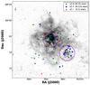 |
Fig. 2 Spatial distribution of the presumably single O-type stars as a function of LC. North is to the top; east is to the left. The circles define regions within 2.4′ of NGC 2070 (central circle) and NGC 2060 (south-west circle). Different symbols indicate LC: III (circles), II (squares), I (triangles). Note that because of crowding a considerable fraction of the sources overlap. Lower opacities again denote sources with an ambiguous LC classification, similar as in Fig. 1. |
2.1. Data preparation
The VFTS data are multi-epoch and multi-setting by nature. To increase the signal-to-noise of individual epochs and to simplify the atmosphere analysis process, we have combined, for each star, the spectra from the various epochs and setups into a single normalized spectrum per object. We provide here a brief overview of the steps taken to reach that goal. We assumed that all stars are single by nature, that is, that no significant RV shift between the various observation epochs needs to be accounted for. This assumption is validated for our sample (see above), which selects either stars with no statistically significant RV variation, or significant but small RV shifts (ΔRV < 20kms-1; hence less than half the resolution element of ~40 kms-1).
For each object and setup, we started from the individual-epoch spectra normalized by Sana et al. (2013) and first rejected the spectra of insufficient quality (S/N< 5). Subsequent steps are:
-
i.
Rebinning to a common wavelength grid, using the largestcommon wavelength range. Step sizes of0.2 Å and0.05 Å are adoptedfor the LR and HR Medusa−Giraffe settings, respectively.
-
ii.
Discarding spectra with a S/N lower by a factor of three, or more, compared to the median S/N of the set of spectra for the considered object and setup;
-
iii.
Computing the median spectrum;
-
iv.
At each pixel, applying a 5σ-clipping around the median spectrum, using the individual error of each pixel;
-
v.
Computing the weighted average spectrum, taking into account the individual pixel uncertainties and excluding the clipped pixels;
-
vi.
Re-normalizing the resulting spectrum to correct for minor deviations that have become apparent thanks to the improved S/N of the combined spectrum. The typical normalization error is better than 1% (see Appendix A in Sana et al. 2013). The obtained spectrum is considered as the final spectrum for a given star and a given observing setup.
-
vii.
The error spectrum is computed through error-propagation throughout the described process.
Once we have combined the individual epochs, we still have to merge the three observing setups. In particular, the averaged LR02 and LR03 spectra of each object are merged using a linear ramp between 4500 and 4525 Å. This implies that below 4500 Å the merged spectrum is from LR02 exclusively and that above 4525 Å it is from LR03. In particular, the information on the He ii λ4541 line present in LR02 is discarded despite the fact that there are twice as many epochs of LR02 than of LR03. This is mainly due to (i) a sometimes uncertain normalization of the He ii λ4541 region in LR02, as the line lies very close to the edge of the LR02 wavelength range; and (ii) the fact that LR02 and LR03 setups yield different spectral resolving power. Hence, we decided against the combination of data that differ in resolving power in such an important line for atmosphere fitting. While we might thus lose in S/N, we gain in robustness. In the 4500–4525 Å transition region, we note that we did not correct for the difference in resolving power between LR02 and LR03. For most objects, no lines are visible there. Finally, HR15N was simply added as there is no overlap.
3. Analysis method
To investigate the atmospheric properties of our sample stars, we obtained the stellar and wind parameters by fitting synthetic spectra to the observed line profiles. This method is described in the following section.
3.1. Atmosphere fitting
The stellar properties of the stars have been determined using an automated method first developed by Mokiem et al. (2005). This method combines the non-LTE stellar atmosphere code fastwind (Puls et al. 2005; Rivero González et al. 2011) with the genetic fitting algorithm pikaia (Charbonneau 1995). It allows for a standardized analysis of the spectra of O-type stars by a thorough exploration of the parameter space in affordable CPU time on a supercomputer (see, Mokiem et al. 2006, 2007a,b; Tramper et al. 2011, 2014).
In the present study, we used fastwind (version 10.1) with detailed model atoms for hydrogen and helium (described in Puls et al. 2005), and in some cases (see below) also for nitrogen (Rivero González et al. 2012a) and silicon (Trundle et al. 2004) as ‘explicit’ elements. Most of the other elements up to zinc were treated as background elements. In brief, explicit elements are those used as diagnostic tools and treated with high precision by detailed atomic models and by means of a co-moving frame transport for all line transitions. The background elements (i.e., the rest) are only needed for the line-blocking/blanketing calculations, and are treated in a more approximate way, though still solving the complete equations of statistical equilibrium for most of them. In particular, parametrized ionization cross sections following Seaton (1958) are used, and a co-moving frame transfer is applied only for the strongest lines, whilst the weaker ones are calculated by means of the Sobolev approximation. For the abundances of these background elements we adopt solar values by Asplund et al. (2005) scaled down by 0.3 dex to mimic the metal deficiency of the LMC (e.g., Rolleston et al. 2002). The abundance of carbon is further adjusted by –1.1 dex (i.e., [C] = 7.0, where [X] is log (X/H)+ 12) and nitrogen by +0.35 dex (i.e., [N] = 7.7), characteristic for the surfacing of CN- and CNO-cycle products (Brott et al. 2011).
The pikaia algorithm was used to evolve a population of 79 randomly drawn initial solutions (i.e., a population consisting of 79 individuals) over 300 generations. The population of each subsequent generation was based on selection pressure (i.e., highest fitness) and random mutation of parameters. Convergence was generally achieved after 30–50 generations, depending on the gravity, with lower-gravity objects requiring more generations to reach convergence. Computing a large number of generations beyond the convergence point allows us to fully explore the shape of the χ2 minimum while further ensuring that the absolute optimum has been identified. The population survival was based on the fitness (F) of the models, computed as:  (1)where
  is the reduced χ2 between the data and the model for line l, wl is a weighting factor, and where the summation is carried out on the number of fitted lines Nl. We adopt unity for all weights, except for He ii λ4200 (w = 0.5) and the singlet transition He i λ4387 (w = 0.25), for reasons discussed in Mokiem et al. (2005).
While the exploration of the parameter space is based on the fitness to avoid a single line outweighing the others, the fit statistics – and the error bars – are however computed using the χ2 statistic, computed in the usual way.  (2)The algorithm makes use of the normalized spectra to derive the effective temperature (Teff), the surface gravity (log g), the mass-loss rate (Ṁ), the exponent of the β-type wind-velocity law (β), the helium over hydrogen number density (later converted to surface helium abundance in mass fraction, Y, through the paper), the microturbulent velocity (νturb) and the projected rotational velocity (νesini). For additional notes on νesini, we refer the reader to Sect. 3.7.1.
While the method, in principle, allows for the terminal wind velocity (ν∞) to be a free parameter, this quantity cannot be constrained from the optical diagnostic lines. Instead, we adopted the empirical scaling of ν∞ with the escape velocity (νesc) of Kudritzki & Puls (2000), taking into account the metallicity (Z) dependence of Leitherer et al. (1992): ν∞ = 2.65 νescZ0.13. In doing so, we corrected the Newtonian gravity as given by the spectroscopic mass for radiation pressure due to electron scattering. In units of the Newtonian gravity, this correction factor is (1−Γe), where Γe is the Eddington factor for Thomson scattering. This treatment of terminal velocity ignores the large scatter that exists around the ν∞ versus νesc relation (see discussions in Kudritzki & Puls 2000; Garcia et al. 2014). However, consistency checks performed in Sect. 3.4.3 indicate that this is not a major issue.
For each star in our sample, up to 12 diagnostic lines are adjusted: He i+iiλ4026, He iλ4387, 4471, 4713, 4922, He iiλ4200, 4541, 4686, Hδ, Hγ, Hβ, and Hα. For a subset of stars (those with the earliest spectral subtypes, and mid- and late-O supergiants), our set of H and He diagnostic lines was not sufficient to accurately constrain their parameters. In these cases, we also adjusted nitrogen lines in the spectra and considered the nitrogen surface abundance to be a free parameter. Specifically, we included the following lines in the list of diagnostic lines used: N iiλ3995, N iiiλ4097, 4103, 4195, 4200, 4379, 4511, 4515, 4518, 4523, 4634, 4640, 4641, N ivλ4058 and N vλ4603, 4619. Tables C.1–C.3 summarize, for each star, the diagnostic lines that have simultaneously been considered in the fit. The fitting results for each object were visually inspected. Residuals of nebular correction were manually clipped, after which the fitting procedure was repeated. The best-fit model and the set of acceptable models, for every star, are displayed in Appendix E (see also Sect. 3.2).
The de-reddened absolute magnitude and the RV of the star are needed as input parameters; the first is used to determine the object luminosity and hence the radius, while the second is used to shift the model and data to the same reference frame. While both Mokiem et al. (2005, 2006, 2007a) and Tramper et al. (2011, 2014) used the V-band magnitude as a photometric anchor, we choose to use the K-band magnitude (MK) to minimise the impact of uncertainties on the individual reddening of the objects in our sample. We determined MK using the VISTA observed K-band magnitude (Rubele et al. 2012), adopting a distance modulus to the Tarantula nebula of 18.5 mag (see Paper I) and an average K-band extinction (AK) of 0.21 mag (Maíz-Apellániz et al., in prep.). The obtained MK values are provided in Table C.4 and C.5, for completeness. As for the RV values we used the measurements listed in Sana et al. (2013).
3.2. Error calculation
The parameter fitting uncertainties were estimated in the following way. For each star and each model, we calculated the probability (P) that the χ2 value as large as the one that we observed is not a result of statistical fluctuation: P = 1−Γ(χ2/ 2,ν/ 2), where Γ is the incomplete gamma function and ν the number of degrees of freedom.
Because P is very sensitive to the χ2 value, we re-normalized all χ2 values such that the best fitting model of a given star has a reduced χ2 ( ) equal to unity. We thus implicitly assumed that the model with the smallest χ2 represents the data and that deviations of the best model’s from unity result from under- or overestimated error bars on the normalized flux. This approach is valid if the best-fit model represents the data, which was visually checked for each star (see Sect. 3.7 and Appendix E). Finally, the 95% confidence intervals on the fitted parameters were obtained by considering the range of models that satisfy P(χ2,ν) > 0.05. The latter can approximately be considered as ± 2σ error estimates in cases where the probability distributions follow a Gaussian distribution.
The finite exploration of parameter space may however result in an underestimate of the confidence interval in the case of poor sampling near the borders P(χ2,ν) = 0.05. As a first attempt to mitigate this situation, we adopt as boundaries of the 95% confidence interval the first models that do not satisfy P(χ2,ν) = 0.05, hence making sure that the quoted confidence intervals are either identical or slightly larger than their exact 95% counterparts. However, for approximately 10% of the boundaries so determined, the results were still leading to unsatisfactory small, or large, upper and lower errors. We then turned to fitting the χ2 distribution envelopes. The left- and right-hand part of the envelopes were fitted separately for all quantities using either a 3rd- or 4th degree polynomial or a Gaussian profile. The intersects of the fitted envelope with the critical χ2 threshold defined above (P(χ2,ν) = 0.05) for the function that best represented the envelope were then adopted as upper- and lower-limit for the 95%-confidence intervals.
The obtained boundaries of the confidence intervals, relative to the best-fit value, are provided in Table C.4. For some quantities and for some stars, these boundaries are relatively asymmetric with respect to the best-fit values. Hence, the total range covered by the 95% confidence intervals needs to be considered to understand the typical error budget in our sample stars, that is, not only the lower- or upper-boundaries. In Fig. 3, we show the distribution of these widths for all model parameters that have their confidence interval constrained (i.e., excluding upper/lower limits). The median values of these uncertainties are 2090 K for Teff, 0.25 dex for log g, and 0.11 for Y. For those sources that have their mass-loss rates constrained, the median uncertainty in log Ṁ is 0.3 dex. For the projected spin velocities it is 44 kms-1. We note that for some sources, the formal error estimates are very small. This is particularly so in cases where nitrogen lines are used as diagnostics, which tend to place stringent limits on the effective temperature, hence indirectly on the surface gravity, and the mass-loss rate. Results related to sources for which nitrogen was included in the analysis have been given a different color in Fig. 3.
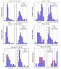 |
Fig. 3 Range of each fitted parameter (left panels of each set) and accompanying range of 95% confidence interval (right panel of each set) in the same unit. Colors have been used to differentiate between stars that have been analyzed using hydrogen and helium lines (HHe) and those for which also nitrogen lines (HHeN) were considered (see also Sect. 3.1). The distributions exclude stars for which only upper/lower limits could be determined, hence the number of stars shown in a panel depends on the parameter that is investigated. In each panel, the median value and the 16th and 84th percentiles are shown using vertical lines. |
3.3. Sources of systematic errors
It is important to stress that the confidence intervals given in Table C.4 represent the validity of the models as well as the formal errors of the fits, that is, uncertainties measuring statistical variability. They do not account for systematic uncertainties, which may be significant. Here we discuss possible sources of this type of uncertainty that may impact the accuracy of our results.
Systematic errors may relate to model assumptions, continuum placement biases, the assumed distance to the LMC, or an uncertain extinction, for example. Regarding the adopted model atmosphere, Massey et al. (2013) performed a by-eye analysis of ten LMC O-type stars using both cmfgen (Hillier & Miller 1998) and fastwind. They report a systematic difference in the derived gravity of 0.12 dex, with cmfgen values being higher. They argue that differences in the treatment of the electron scattering wings might explain the bulk of this difference, a treatment that is more refined in cmfgen. A systematic error in the normalization of the local continuum may also impact the gravity estimate. If by-eye judgement would place it too high by 1% (where the typical normalization error is better than 1%; see Sect. 2.1) for all relevant diagnostic lines, this would lead to a gravity that is higher by less than 0.1 dex. We do not, however, anticipate such a large systematic normalization error. The distance to the LMC is accurate to within 2% (Pietrzyński et al. 2013). We adopt a mean K-band extinction of 0.21 mag (see Sect. 3.1). Typical deviations of this mean value are not larger than 0.1 mag (Maíz-Apellániz et al., in prep.), hence correspond to an uncertainty in the luminosity of less than 10%.
Other systematic uncertainties may be present; for instance model assumptions that impact both a fastwind and cmfgen analysis. Examples are the neglect of macro-turbulence or the assumption of a spherical and constant mass-loss rate outflow.
Systematic (quantifiable and non-quantifiable) errors will impact the formal confidence intervals discussed in Sect. 3.2. In those cases where the quoted confidence intervals are approximately equal to their respective medians or larger, the systematic errors will likely contribute modestly to the total uncertainties. In cases where the formal errors are small, we caution the reader that systematic uncertainties may be larger than the statistical uncertainties presented in Table C.4.
3.4. Consistency checks
Here we compare aspects of the properties obtained for our sample stars to those of other O-type sub-samples analyzed in the VFTS.
3.4.1. O V and IV stars
To test the consistency of our results with the atmosphere fitting methods applied to O-type dwarfs within the VFTS, we selected a subset of 66 stars from Paper XIII. We computed the stellar properties by means of our atmosphere fitting approach. The fitting approach in Paper XIII also made use of fastwind models, but applied a grid-based tool, where the absolute flux calibration relied on the V-band magnitude. The values that we obtained are in agreement with those of Paper XIII. Specifically, the weighted mean of the temperature difference (ΔTeff [Paper XIII− this study]) and the 1σ dispersion around the mean value are 0.69 ± 0.33 kK and 1.21 ± 0.37 kK, respectively. The weighted mean of the luminosity difference (Δlog L/L⊙[Paper XIII− this study]) and its 1σ dispersion are 0.08 ± 0.02 and 0.07 ± 0.02. Similarly, the weighted mean of the difference in gravity between both fitting approaches (Δlog g[Paper XIII− this study]) and its 1σ dispersion are 0.16 ± 0.04 and 0.09 ± 0.04 (if g is measured in units of cm s-2). Typical errors on the temperature, gravity, and luminosity in both methods are 1 kK, 0.1 dex, and 0.1 dex, respectively, that is, of the same order as the mean differences. Hence, this comparison does not reveal conspicous discrepancies in temperature and luminosity. Possibly, a modest discrepancy is present in gravity.
3.4.2. O9.7 stars
The spectral analysis of the O9.7 subtype is complicated as the He ii lines become very weak, hence small absolute uncertainties may have a larger impact on the determination of the effective temperature. For early-B stars, one also relies on Si iii and iv lines as a temperature diagnostic (see, e.g., McEvoy et al. 2015). We performed several checks to assess the reliability of our parameters for the late O stars. For four stars; VFTS 035 (O9.5 IIn), 235 (O9.7 III), 253 (O9.7 II), and 304 (O9.7 III), we used fastwind models that include Si iii λ4552, 4567, 4574, Si iv λ4128, 4130, and Si v λ4089, 4116 as extra diagnostics. The temperatures and gravities that we then obtain agree within 400 K and 0.28 dex, respectively, that is, within typical uncertainties, suggesting that the lack of silicon lines in our automated fastwind modeling does not introduce systematic effects.
One may also compare to atmosphere models that assume hydrostatic equilibrium, that is, that neglect a stellar wind. This is done in McEvoy et al. (2015) for two O9.7 sources, VFTS 087 (O9.7 Ib-II) and 165 (O9.7 Iab), where fastwind analyses are compared to tlusty analyses (Hubeny 1988; Hubeny & Lanz 1995; Lanz & Hubeny 2007). Here fastwind settles on temperatures that are 1000 K higher, which is within the uncertainties quoted. This is accompanied by 0.07 dex higher gravities, which is well within the error range. We also compared to preliminary tlusty results for some of the stars analyzed here (Dufton et al., in prep.); namely VFTS 113, 192, 226, 607, 753, and 787, all O9.7 II, II−III, III sources. The weighted mean of the temperature difference (ΔTeff [tlusty − this study]) and the associated 1σ dispersion are − 1.95 ± 1.26 kK and 0.81 ± 4.15 kK. This offset is similar to that reported by Massey et al. (2009). Similarly, the weighted mean of the difference in log g and the associated 1σ dispersion are − 0.29 ± 0.07, and 0.07 ± 0.04. These differences are larger than one might expect and warrant caution. For LMC spectra of the quality studied here, systematic errors in Teff and gravity between fastwind and tlusty, at spectral type O9.7, can not be excluded.
3.4.3. The most luminous stars
Twelve objects in our sample are in common with Paper XVII, which analyzed the stars with the highest masses and luminosities. These stars are VFTS 016, 064, 171, 180, 259, 267, 333, 518, 566, 599, 664, and 669. VFTS 064, 171, and 333 are, however, excluded from the present comparison because our obtained fits were rated as poor quality (see Sect. 3.6). For the remaining nine stars, the values obtained in this paper agree well with those of Paper XVII. The weighted mean of the temperature difference (ΔTeff [Paper XVII− this study]) and the associated 1σ dispersion of this set of nine stars are 1.52 ± 0.18 kK and 1.82 ± 0.35 kK. The weighted mean of the luminosity difference (Δlog L/L⊙ [Paper XVII− this study]) and its 1σ dispersion are 0.09 ± 0.02 and 0.06 ± 0.01. The gravities cannot be compared in a similar way as they were held constant in Paper XVII. For this reason, the present results are to be preferred for stars in common with Bestenlehner et al. (2014).
For the small number of stars for which ν∞ could actually be measured in Paper XVII, the terminal velocities are consistent with those that we estimated from the ν∞/ νesc relation. Regarding the unclumped mass-loss rates, the weighted mean of the log Ṁ differences (Δlog Ṁ [Paper XVII− this study]), and its 1σ dispersion, are − 0.03 ± 0.23 M⊙/yr, and 0.21 ± 0.19 M⊙/yr, indicating the absence of systematics between the results of both studies. Finally, previous optical and ultraviolet analysis of VFTS 016 had constrained ν∞ to 3450 ± 50kms-1 (Evans et al. 2010), in satisfactory agreement with the value of  kms-1 that we derived from our best-fit parameters using the scaling with νesc.
3.5. Derived properties
In addition to ν∞ (see Sect. 3.1), several important quantities can be derived from the best-fit parameters: the bolometric luminosity L, the stellar radius R, the spectroscopic mass Mspec, and the modified wind-momentum rate Dmom = Ṁv∞ (R/R⊙)1/2. The latter quantity provides a convenient means to confront empirical with predicted wind strengths as Dmom is expected to be almost independent of mass (e.g., Kudritzki & Puls 2000, see Sect. 4.5). To determine the radius, the theoretical fluxes have been converted to K-band magnitude using the 2MASS filter response function1 and the absolute flux calibration from Cohen et al. (2003). The values of the parameters mentioned above for our sample stars together, with their corresponding 95% confidence interval, are provided in Table C.4 as well.
3.6. Binaries and poor quality fits
VFTS 064, 093, 171, 332, 333, and 440 have been subjected to further RV monitoring and are now confirmed to be spectroscopic binaries (Almeida et al. 2017, see also Appendix D). In VFTS, they all showed small but significant radial velocity variations (ΔRV ≤ 20kms-1; Sana et al. 2013). Walborn et al. (2014) noted these six objects as having a somewhat problematic spectral classification. Interestingly, our fits of these six stars often implied a helium abundance significantly lower than the primordial value, which may be the result of line dilution by the continuum of the companion. We decided to discard these stars from our discussion, opting for a sample of 72−6 = 66 high-quality fits only and minimizing the risk of misinterpretations. We do provide the obtained parameters and formal uncertainties of these six stars in Table C.4 but warn against possible systematic biases.
All other spectral fits were screened by eye to assess their quality. We concluded that all fits were acceptable within the range of models that pass our statistical criteria except those of six objects without LC (VFTS 145, 360, 400, 446, 451, and 565). We also provide the obtained parameters of these six stars in Table C.5 but warn that they may not be representative of the stars physical parameters as their fits have limited quality.
3.7. Limitations of the method
We discuss two limitations of the method in more detail, that is, the neglect of macro-turbulence and the lack of a diagnostics that allows us to constrain the spatial velocity gradient of the outflow.
3.7.1. Extra line-broadening due to macro-turbulent motions
When comparing the models with the data, we take into account several sources of spectral line broadening: intrinsic broadening, rotational broadening, and broadening due to the instrumental profile. However, we do not take into account the possibility of extra-broadening as a result of macro-turbulent motions in the stellar photosphere (e.g., Gray 1976). This approach is somewhat different to that of Paper XII, in which a Fourier transform method was used to help differentiate between rotation and macro-turbulent broadening, neglecting intrinsic line broadening and given a model for the behavior of macro-turbulence (we refer to Paper XII for a discussion).
Appendix A compares the rotation rates of the sample of 66 stars obtained through both methods. The systematic difference (Δ νesini [this study – Paper XII]) is approximately 7 kms-1 with a standard deviation of approximately 21 kms-1. This is within the uncertainties discussed in Paper XII. At projected spin velocities below 160 kms-1 the present measurements may overestimate νesini by up to several tens of kms-1 in cases where macro-turbulence is prominent. Though, the best of our knowledge, there are no theoretical assessments of the impact of macro-turbulence on the determination of the stellar parameters, we do not expect the differences in νesini to affect the determination of other stellar properties in any significant way as the νesini measurements of both methods are within uncertainties.
3.7.2. Wind-velocity law
The spatial velocity gradient, measured by the exponent β of the wind-velocity law becomes unconstrained if the diagnostic lines which are sensitive to mass-loss rate (Hα and He iiλ4686) are formed close to the photosphere. In such cases, the flow velocity is indeed still low compared to ν∞. In an initial determination of the parameters, we let β be a free parameter in the interval [0.8, 2.0]. In approximately half of the cases, the fit returned a central value for β larger than 1.2 and with large uncertainties. From theoretical computations, such a large acceleration parameter is not expected for normal O stars and we identified these sources as having an unconstrained β. Given the large percentage of stars that fell in this category and the potential impact of β on the derived mass-loss rate, we decided to adopt β = 0.9 for giants and 0.95 for bright giants and supergiants, following theoretical predictions by Muijres et al. (2012). For the 31 O stars that could not be assigned a LC, we adopted the canonical value β = 1 (see Table C.5). We will discuss the impact of this assumption in Sect. 4.5.
4. Results and discussion
We discuss our findings for the effective temperature, gravity, helium abundance, mass loss, and mass, and place these results in the broader context of stellar evolution, mass-loss behavior, and mass discrepancy.
4.1. Effective temperature vs. spectral subtype calibrations
Figure 4 plots the derived effective temperature for 53 giants, bright giants and supergiants as a function of spectral subtype. This sample of 53 stars corresponds to the high-quality fits (66 stars) minus the stars that have a somewhat ambiguous luminosity classification (17 minus the newly confirmed binaries VFTS 093, 171, 332, and 333 fits, hence 13 stars; we refer to Sects. 2 and 3.6). For LC III and LC II stars, the scatter at late spectral type is too large to be solely explained by measurement errors and may thus also reflect intrinsic differences in gravity, hence in evolutionary state (for a discussion, see Simón-Díaz et al. 2014). Added to the figure are results for 18 LC III to I LMC stars by Mokiem et al. (2007b). These were analyzed using the same fitting technique, save that these authors did not use nitrogen lines in cases where either He i or He ii lines were absent (see Sect. 3.1). Both our sample and that of Mokiem et al. yield results that are compatible with each other, therefore we combine both samples in the remainder of this section.
Though the overall trend in Fig. 4 is clearly that of a monotonically decreasing temperature with spectral subtype, such a trend need not necessarily reflect a linear relationship. Work by Rivero González et al. (2012a,b) for early-O dwarfs in the LMC, for instance, suggests a steeper slope at the earliest subtypes (O2-O3). This seems to be supported by first estimates of the properties of O2 dwarfs in the VFTS by Sabín-Sanjulián et al. (2014). The presence of such an upturn starting at spectral sub-type O4 is not confirmed in Fig. 4. The three O2 III stars (all from Mokiem et al.) do show a spread that may be compatible with a steeper slope for giants but such an increased slope is not yet needed at subtype O3. Furthermore, the only two O2 I and O3 I stars in Fig. 4 are perfectly compatible with a constant slope down to the earliest spectral sub-types for the supergiants. In regards to the insufficient number of stars, to fully test for the presence of an upturn at subtype O2, we limit our Teff-SpT calibrations to subtypes O3 and later.
 |
Fig. 4 Effective temperature vs. spectral subtype for the O-type with well defined LC (see main text). The lower-opacity symbols give the results for the sample of LMC stars investigated by Mokiem et al. (2007b). |
Teff −SpT linear-fit parameters and their 1σ error bars derived for stars with spectral subtypes O3 to O9 in the combined sample (see text).
A shallowing of the Teff-SpT relation at subtypes later than O9 (relative to the O3-O9 regime) is also relatively conspicuous in Fig. 4. We too exclude this regime from the relations given below, also because the luminosity classification of this group in particular may be debated (see Sect. 4.2). We thus aim to derive Teff-SpT relations for LMC O-type stars in the regime O3-O9. To do so, we used a weighted least-square linear fit to adjust the relation  (3)where the spectral subtype is represented by a real number, for example, SpT = 6.5 for an O6.5 star. Figure 5 shows these linear fits for our sample and that of Mokiem et al. (2007a) combined, for each luminosity class separately. The fit coefficients and their uncertainties are provided in Table 1.
A comparison of our combined LC III, II and I relations with theoretical results for a LMC metallicity is not feasible as, to our knowledge, such predictions are not yet available. One may anticipate that a LMC calibration would be shifted up to higher temperatures, as, in a lower metallicity environment, the effects of line blocking/blanketing are less important than in a high-metallicity environment. Thus, fewer photons are scattered back, contributing less to the mean intensity in those regions where the He i lines are formed. Consequently, a higher Teff is needed to reach the same degree of ionization for stars in the LMC compared to those with a higher metal abundance (which have stronger blocking/blanketing, see Repolust et al. 2004). In Fig. 5, we compare our results to the LC III and I empirical calibrations of Martins et al. (2005, their Eq. (2)) for Galactic stars. Below we discuss the results for LC III, II, and I separately:
-
Giants (LC III): the slope of theTeff-SpT relation for giants is in excellent agreement with the (observational) Martins et al. (2005) calibration, though an upward shift of approximately 1 kK is required to account for the lower metallicity. Doran et al. (2013) report that a +1 kK shift is required to match the LMC dwarfs, but that no shift seems required for O-giants. Our results suggest that this upward shift should be applied to this category as well.
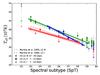
Fig. 5 Effective temperature vs. spectral subtype but now displaying fits that combine our sample with that of Mokiem et al. (2007b): CS = Combined sample (see main text). Stars with spectral subtype O2-3 or later than O9 have been plotted with lower opacity. The dashed lines give the theoretical calibrations of Martins et al. (2005) for Galactic class III and I stars. The leading number in the legend refers to the total number of O3-O9 stars for which the fit has been derived. The trailing number refers to the total number of stars in each sample.

Fig. 6 log gc vs. log Teff (upper panel) and spectroscopic Hertzsprung-Russell (lower panel) diagrams of the O-type giants, bright giants, and supergiants, where
 (see Sect. 4.2). Symbols and colors have the same meaning as in Fig. 5. Evolutionary tracks and isochrones are for models that have an initial rotational velocity of approximately 200 kms-1 (Brott et al. 2011; Köhler et al. 2015). In the lower panel, the right-hand axis gives the classical Eddington factor Γe for the opacity of free electrons in a fully ionized plasma with solar helium abundance (cf. Langer & Kudritzki 2014). The horizontal line at log L/ L⊙ = 4.6 indicates the location of the corresponding Eddington limit. The dashed straight lines are lines of constant log g as indicated. Lower opacities of the green and blue symbols and the numbers in parentheses in the legend have the same meaning as in Fig. 1.
 -
Bright giants (LC II): the Teff-SpT relation for the bright giants is relatively steep, and crosses the relations for the giants and supergiants. As explained in the notes for individual stars (Appendix D), the spectra of some of these stars are peculiar. We also note that in the Hertzsprung-Russell diagram the O II stars do not appear to constitute a distinct group intermediate between the giants and supergiants (see Figs. 6 and 9); rather, they mingle between the O V and I stars. This might explain their behavior in Fig. 5 and implies that one should be cautious in using this relation as a calibration. We recommend to refrain from doing so and to wait until more data become available.
-
Supergiants (LC I): our supergiant sample is smaller than that of the giants and some O I stars have peculiar spectra (Appendix D), yet it is the largest LMC supergiants sample assembled so far and hence worthy of some in-depth discussion. As also observed at Galactic metallicity (Martins et al. 2005), our derived Teff-SpT relation for supergiants is shallower than that for giants. The slope for the supergiants is even more shallow at LMC than obtained by Martins et al. in the Milky Way. Furthermore, the upward shift measured for LMC V and III stars compared to those in the Galaxy is not seen for the supergiants. If anything, a downward shift is present at the earliest spectral types. Within uncertainties however, one may still accept the Galactic-metallicity relation derived for LC I by Martins et al. as a reasonable representation of the LMC supergiants. A larger sample would be desirable to confirm or discard these preliminary conclusions as well as to investigate the physical origin of the different metallicity effects for LC I objects compared to LC V and III stars.
4.2. Gravities and luminosity classification
We present the Newtonian gravities graphically using the log gc − log Teff diagram and the spectroscopic Hertzsprung-Russell (sHR) diagram (Fig. 6). In doing so, the gravities were corrected for centrifugal acceleration using log gc = log [ g + (νesini)2/R ] (see also Herrero et al. 1992; Repolust et al. 2004). The sHR diagram shows L versus Teff.  is proportional to L/M, thus to Γe/κ, where κ is the flux-mean opacity (see Langer & Kudritzki 2014). For a fixed κ, the vertical axis of this diagram thus sorts the stars according to their proximity to the Eddington limit: the higher up in the diagram the closer their atmospheres are to zero effective gravity (see also Castro et al. 2014).
Figure 6 shows both diagrams for our stars. We have supplemented them with VFTS LC V stars analyzed in Paper XIII. Stars that evolve away from the ZAMS increase their radii, and hence decrease their surface gravity. Therefore, it is expected that the different luminosity classes are separated in these diagrams, that is, stars assigned a lower roman numeral are located further from the ZAMS. This behavior is clearly visible for the supergiants that seem to be the most evolved stars along the main sequence. The bright giants mingle with the supergiants, though some, at 25−30 M⊙ reside where the dwarf stars dominate. They do not appear to form a well defined regime intermediate between giants and supergiants, though it should be mentioned that the sample size of these stars is small.
At initial masses of approximately 60 M⊙ and higher, giants and bright giants appear closer to the ZAMS. This is the result of a relatively high mass-loss rate, as the morphology of He ii λ4686 – the main diagnostic used to assign luminosity class – traces wind density. At initial masses in-between approximately 18 M⊙ and 60 M⊙, the dwarf phase clearly precedes the giant and bright giant phase. However, at lower initial masses the picture is more complicated. Here a group of late-O III and II stars populate the regime relatively close to the ZAMS, where dwarf stars are expected. The properties of these stars are indeed more characteristic for LC V objects; they have gravities log gc between 4.0 and 4.5 and radii of approximately 5−8 R⊙. Consequently, their absolute visual magnitudes are fainter than calibrations suggest (Walborn 1973). In addition, these objects display higher spectroscopic masses than evolutionary masses (see Sect. 4.6 and Fig. 12).
What could explain this peculiar group of stars? Though we do not want to exclude the possibility that these objects belong to a separate physical group, we do find that they populate a part of the HRD where few dwarf O stars are actually seen (see Sect. 4.4). A simple explanation may thus be an intricacy with the LC classification.
The spectral classification in the VFTS is described in Walborn et al. (2014). For the late-O stars, following, for example Sota et al. (2011), it relies on the equivalent width ratio He iiλ4686/He iλ4713 as its primary luminosity criterion. The relative strength of Si iv to He i absorption lines may serve as a secondary criteria, a measure that is somewhat susceptible to metallicity effects (see Walborn et al. 2014). The Si iv/He i ratio is however the primary classifier in early-B stars.
Though He iiλ4686/He iλ4713 is the primary criterion in the VFTS, the group of problematic stars being discussed here have Si iv weaker than expected for LC III, favoring a dwarf or sub-giant classification. Indeed, it is often for this reason that the classification of these stars is lower rated in Walborn et al. (2014). Other reasons for the problematic classification of these stars may be relatively poor quality spectra and an inconspicuous binary nature. Regarding the latter possibility, we mention that a similar behavior is seen in some Galactic O stars, as discussed in Sota et al. (2014) and in the third paper of the Galactic O-Star Spectroscopic Survey series (Maíz Apellániz et al. 2016). More specifically, it is seen in the A component of σ Ori AB, that this star itself is a spectroscopic binary. For this system, Simón-Díaz et al. (2011, 2015) find that the spectrum is the composite of that of an O9.5 V and B0.5 V star. Further RV monitoring has indeed revealed that some of these late-O III and II stars are genuine spectroscopic binaries (see annotations in Appendix D).
4.3. Helium abundance
Figure 7 shows the helium mass fraction Y as a function of νesini (top panel) and log gc (bottom panel). Most of the stars in our sample agree within their 95% confidence intervals with the initial composition of the LMC, Y = 0.255 ± 0.003, which has been derived by scaling the primordial value (Peimbert et al. 2007) linearly with metallicity (Brott et al. 2011).
Table 2 summarizes the frequency of stars in the total sample and in given sub-populations that have Y larger, by at least 2σY, than a specified limit. We find that 92.4% of our 66-star sample does not show a clear signature of enrichment given the uncertainties, that is, has Y−2σY ≤ 0.30. Five stars (VFTS 046, 180, 518, 546, and 819), hence 7.6% of our sample, meet the requirement of Y−2σY> 0.30 for a clear signature of enrichment. Interestingly, all these sources have a projected spin velocity less than 200 kms-1 (see upper panel Fig. 7). The lower panel of Fig. 7 plots helium abundance as a function of surface gravity. All sources with Y−2σY> 0.35 have gravities less than or equal to 3.83 dex, though not all sources that have such low gravities have Y−2σY> 0.35. This conclusion does not change if we take log gc instead.
Frequency of stars from different sub-samples that display a helium abundance by mass (Y) larger than the specified limit by at least 2σY.
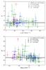 |
Fig. 7 Helium mass fraction Y versus νesini (upper panel) and log gc (lower panel). Symbols and colors have the same meaning as in Fig. 5. Gray diamonds denote stars with LC III to I from Mokiem et al. (2007a). The purple dashed line at Y = 0.255 defines the initial composition for LMC stars; the gray bar is the 3σ uncertainty in this number. |
We ran Monte-Carlo simulations to estimate the number of spuriously detected He-rich stars in our sample, that is, the number of stars that have normal He-abundance but for which the high Y value obtained may purely result from statistical fluctuations in the measurement process. Given our sample size and measurement errors, we obtained a median number of two spurious detections. Within a 90% confidence interval, this number varies between zero and three. While some detections of He-rich stars in our sample may thus result from statistical fluctuations, it is unlikely that all detections are spurious.
Further, some of the stars appear to have a sub-primordial helium abundance. This is thought to be unphysical, possibly indicating an issue with the analysis such as continuum dilution. Continuum dilution may be caused by multiplicity (either through physical companions or additional members of an unresolved stellar association) and nebular continuum emission, contributing extra flux in the Medusa fiber. In the former case, the extra continuum flux of the companion may weaken the lines, essentially mimicking an unrealistically low helium content. Alternative explanations may be linked to effects of magnetic fields and of (non-radial) pulsations, though, at the present time, little is known about the impact of these processes on the (apparent) surface helium abundance.
4.3.1. The dependence of Y on the mass-loss rate and rotation rate
As a relatively low surface gravity (log gc ≤ 3.83) seems a prerequisite for surface helium enrichment, envelope stripping through stellar winds may be responsible for the high Y. To investigate this possibility we plot Y versus the mass-loss rate relative to the mass of the star (Ṁ/M) in Fig. 8. Here, we adopt Mspec as a proxy for the mass; using the evolutionary mass Mevol yields similar results. The quantity Ṁ/Mspec is the reciprocal of the momentary stellar evaporation timescale. Also plotted are the set of 26 very massive O, Of, Of/WN, and WNh stars (VMS) analyzed in Paper XVII. At log (Ṁ/M) ≳ −7, these stars display a clear correlation with helium abundance. This led Bestenlehner et al. (2014) to hypothesize that, in this regime, mass loss is exposing helium enriched layers.
To explore this further, we compare the data with the main-sequence predictions for Y versus Ṁ/M by Brott et al. (2011) and Köhler et al. (2015) for massive stars in the range of 30−150 M⊙. So far, this is the only set of tracks at LMC metallicity that includes rotation and that covers a wide range of initial spin rates. The plotted tracks have been truncated at 30 kK, that is, approximately where the stars evolve into B-type (super)giants and thus leave our observational sample.
The empirical mass-loss rates used to construct this diagram (i.e., the data points) assume a homogeneous outflow. In Sect. 4.5 we discuss wind clumping, there we point out that for the stars studied here our optical wind diagnostics can be reconciled with wind-strength predictions as used in the evolutionary calculations if the empirical log Ṁ values are reduced by ~0.4 dex. Hence, in Fig. 8, the empirical measurements of log (Ṁ/M) should also be reduced by this amount. Regarding the log (Ṁ/M) measurements of Paper XVII (the red squares in Fig. 8), these should also be shifted to lower values. Yet, as the mass estimates obtained in Paper XVII were upper limits and not actual measurements, the reduction in log (Ṁ/M) of these stars may be limited to ~0.2−0.4 dex assuming similar clumping properties in Of, Of/WN and WNh stars as applied for O stars.
The upper panel in Fig. 8 shows tracks for initial spin velocities close to 200 kms-1. Within the framework of the current models, no significant enrichment is expected in the O or WNh phase, with the possible exception of stars initially more massive than ~150 M⊙. We add that mass-loss prescriptions adopted in the evolutionary tracks discussed here account for a bi-stability jump at spectral type B1.5, where the mass-loss rate is predicted to strongly increase (Vink et al. 1999). Beyond the bi-stability jump stars initially more massive than ~60−80 M⊙ do show strong helium enrichment but, by then, the stars have already left our O III-I sample.
The lower panel in Fig. 8 shows O-star tracks for an initial spin rate of approximately 300 kms-1. In this case, the Köhler et al. (2015) models do predict an increase in Y during the O star phase for initial masses ~60 M⊙ and up. Initially, they spin so fast that rotationally-induced mixing prevents the build-up of a steep chemical gradient at the core boundary. The lack of such a barrier explains the initial rise in Y. However, as a result of loss of angular momentum via the stellar wind and the associated spin-down of the star, a chemical gradient barrier may develop during its main-sequence evolution. Such a gradient effectively acts as a “wall” inhibiting the transport of helium to the surface. This can be seen in Fig. 8 as a flattening of the Y increase with time. Once such a barrier develops, the star starts to evolve to cooler temperatures, an evolution that was prohibited in the preceding phase of quasi-chemically homogeneous evolution. Once redward evolution commences, stripping of the envelope by mass loss may aid in increasing the surface helium abundance. In our tracks this is only significant for initial masses 125 M⊙ and up.
Finally, our findings might indicate that the current implementation of rotational mixing and wind stripping in single-star models is not able to justify the Y abundances of most of the helium enriched stars in our sample. In the following subsection we combine the constraints on the helium abundance with the projected spin rate of the star and its position in the Hertzsprung-Russell diagram to further scrutinize the evolutionary models.
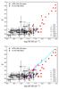 |
Fig. 8 Helium mass fraction Y versus the empirical (unclumped) mass-loss rate relative to the stellar mass (Ṁ/M) for our sample stars with their respective 95% confidence intervals. Added to this is the set of very massive luminous O, Of, Of/WN and WNh stars analyzed in Paper XVII, excluding the nine stars in common with this paper. Also shown are evolutionary tracks by Brott et al. (2011) and Köhler et al. (2015) for stars with initial spin rates of approximately 200 kms-1 (upper panel) and 300 kms-1 (lower panel) with dots every 1 Myr of evolution. These tracks are truncated at 30 kK, which is approximately the temperature where the stars evolve into B-type objects and thus are no longer part of our observational sample. |
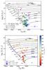 |
Fig. 9 Two versions of the Hertzsprung-Russell diagram. In the top panel our sample of single O-type giants and supergiants is supplemented with the dwarf O star sample of Paper XIII and the sample of very massive Of and WNh stars by Paper XVII. We exclude the results of Paper XVII for the nine stars in common with this paper and adopted our results (see Sect. 3.4.3). Symbols and colors have the same meaning as in Fig. 6. The lower panel only contains the sample studied here. The symbol shapes in the lower panel show three categories of helium mass fraction, that is, not enriched (squares), moderately enriched (triangles), and enriched (stars). The symbol colors refer to their projected rotational velocity (see color bar on the right). Evolutionary tracks and isochrones are for models that have an initial rotational velocity of approximately 200 kms-1 (Brott et al. 2011; Köhler et al. 2015). Iso-helium lines for different rotational velocities are from Köhler et al. (2015) and are color-coded using the color bar. |
4.4. Hertzsprung-Russell diagram
In this section, we explore the evolutionary status of our sample stars by means of the Hertzsprung-Russell diagram (see Fig. 9). Two versions of the HRD are shown in Fig. 9. In the top panel, our sample of giants, bright giants, and supergiants is complemented with the VFTS samples of very massive stars (VMS) from Paper XVII and of LC V stars from Paper XIII. VMS populate the upper left part of the HRD. Giants, bright giants, and supergiants are predominantly located in between the 2 and 5 Myr isochrones while dwarfs are found closer to the ZAMS. The location of LC V stars compared to III, II and I stars reflects their higher surface gravities as shown in Fig. 6. At the lowest luminosities, we note a predominance of LC III and II stars and an absence of LC V stars. As discussed in Sect. 4.2 this may reflect a classification issue.
The positions of the O stars in the HRD do not reveal an obvious preferred age but rather show a spread of ages, supporting findings of De Marchi et al. (2011), Cioni (2016), and Sabbi et al. (2016). HRDs of each of the spatial sub-populations defined in Sect. 2 do not point to preferred ages either (see Appendix B and Fig. B.1), suggesting that star formation has been sustained for the last 5 Myr at least throughout the Tarantula region. We stress that the central 15′′ of Radcliffe 136, the core cluster of NGC 2070, is excluded from the VFTS sample. The age distribution of the Tarantula massive stars will be investigated in detail in a subsequent paper in the VFTS series (Schneider et al., in prep.).
In the lower panel of Fig. 9, we include information on Y and νesini for our sample stars. We also include iso-helium lines for Y = 0.30 and 0.35 as a function of initial rotational velocity (see figure 10 of Köhler et al. 2015). According to these tracks, main-sequence stars initially less massive than ~100 M⊙ with initial rotation rates of 200 kms-1 or less are not expected to show significant helium surface enrichment, that is, Y< 0.30. Stars with an initial rotation rate of 300 kms-1 are only supposed to reach detectable helium enrichment in the O star phase if they are initially at least 60 M⊙. Helium enrichment is common for 20 M⊙ stars and up if they spin extremely fast at birth (νe > 400kms-1). Below we discuss how this compares with our sample stars.
First, our finding that all helium enriched stars have a present day projected spin rate of less than 200 kms-1 (see also Fig. 7) appears at odds with the predictions of the tracks referred to above. In the LMC, significant spin-down due to angular-momentum loss through the stellar wind and/or secular expansion is only expected by Brott et al. (2011) and Köhler et al. (2015) for stars initially more massive than ~40 M⊙, once these objects evolve into early-B supergiants (Vink et al. 2010). Only for much higher initial mass are the winds sufficiently strong to cause rotational braking during the O-star phase. This could perhaps help explain the two highest-luminosity He-enriched objects, VFTS 180 and 518, though in the context of our models this requires an initial spin of 400 kms-1 and wind strengths typical for at least ~125 M⊙ stars. Their evolutionary masses are at most 50 M⊙. It is furthermore extremely unlikely that the remaining three He-enriched stars at lower luminosity (having initial masses <40 M⊙) spin at 400 kms-1 and are all seen almost pole-on. For the two hot He-enriched stars VFTS 180 and 518 we included a set of nitrogen diagnostic lines (see Sect. 3.1). Interestingly, we find that they are nitrogen enriched as well (i.e., [N] > 8.5). A thorough nitrogen analysis of the full sample is presented by Grin et al. (2017, see also Summary).
If indeed these are main-sequence (core H-burning) stars that live their life in isolation, rotational mixing, as implemented in the evolutionary predictions employed here, cannot explain the surface helium mass fraction in this particular subset of stars. This would point to deficiencies in the physical treatment of mixing processes in the stellar interior.
Alternatively, the high helium abundances could point to a binary history (e.g., mass transfer or even merger events; see e.g., de Mink et al. 2014; Bestenlehner et al. 2014) or post-red supergiant (post-RSG) evolution. Concerning the former option, one of these sources is VFTS 399, which has been identified as an X-ray binary by Clark et al. (2015). Concerning the latter option, LMC evolutionary tracks that account for rotation and that cover the core-He burning phase have been computed by Meynet & Maeder (2005). These tracks indicate that a brief part of the evolution of stars initially more massive than 25 M⊙ may be spent as post-RSG stars hotter than 30 000 K. However, these exceptional stars would be close to the end of core-helium burning and feature much higher helium (and nitrogen) surface abundances.
Second, while we have only a few fast rotators, these stars do not seem to be helium enriched (see again Fig. 7). All of them have masses below 20 M⊙, therefore no significant helium enrichment is expected, in agreement with our measurements. If such fast rotators are spun-up secondaries resulting from binary interaction (e.g., Ramírez-Agudelo et al. 2013; de Mink et al. 2013), then the interaction process should have been helium neutral. Some of the stars appear to have sub-primordial helium abundances. This could also be an indication of present-day binarity (see Sect. 4.3). Among them are some of the fastest spinning objects, consistent with the latter conjecture.
4.5. Mass loss and modified wind momentum
In the optical, the mass-loss rate determination relies on wind infilling in Hα and He ii λ4686. These recombination lines are indeed sensitive to the invariant wind-strength parameter Q = Ṁ/ (Rν∞)3/2 that is inferred from the spectral analysis (see, e.g., Puls et al. 1996; de Koter et al. 1998). For approximately 40% of our sample only upper limits on Ṁ can be determined. These stars mostly have Ṁ < 10-7 M⊙ yr-1 and log (L/L⊙) < 5.0. This group of relatively modest-mass stars (Mspec ≤ 25 M⊙) is excluded from the analysis presented in this section.
To facilitate a comparison of the mass-loss rates of the remaining stars with theoretical results, we use the modified wind momentum luminosity diagram (WLD; Fig. 10). The modified wind momentum Dmom is defined in Sect. 3.5. For a given metallicity, Dmom is predicted to be a power-law of the stellar luminosity, that is,  (4)where x is the inverse of the slope of the line-strength distribution function corrected for ionization effects (Puls et al. 2000). For a metal content of solar down to ~1/5th solar, x and D0 do not depend on spectral type for the parameter range considered here, which allows for a simple (i.e., power-law) prescription of the mass-loss metallicity dependence.
The top panel of Fig. 10 shows the WLD for our sample, where Dmom is in the usual units of g cm s-2. Upper limits for the weak-wind stars are also shown (see legend). A linear fit to the stars for which we have a constraint on the mass-loss rate is given in blue, with the shaded blue area representing the uncertainty as a result of errors in Dmom. Also plotted in the figure are the results of Mokiem et al. (2007b) for 38 stars in total in the LMC (sub-)sample, 16 of which are in N11. Our results exhibit somewhat higher Dmom values than those of Mokiem et al. (2007b). The reason for this discrepancy is illustrated in the lower panel, where we have repeated our analysis applying identical fitting constraints as Mokiem et al. This implies that we let β be a free parameter and have removed the nitrogen lines from our set of diagnostics. In that case, we recover essentially the same result. As pointed out in Sect. 3.7, allowing the method to constrain the slope of the velocity law yields higher β values compared to the adopted values, that is, those based on theoretical considerations, for a substantial fraction of the stars. A shallower velocity stratification (that is, a higher β) in the Hα and He ii λ4686 forming regions corresponds to a higher density for the same Ṁ. As the recombination lines depend on the square of the density, the emission will be stronger (at least in the central regions of the profile). Hence, to fit the profiles compared to a lower β, one needs to reduce the mass loss in the models.
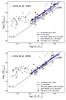 |
Fig. 10 Modified wind momentum (Dmom) vs. luminosity diagram. The dashed lines indicate the theoretical predictions of Vink et al. (2001) for homogeneous winds. Top panel: the empirical fit for this work and Mokiem et al. (2007a) (both for L/L⊙> 5.0) in shaded blue and gray bars, respectively. For stars with L/L⊙ ≤ 5.0, only upper limits could be constrained. These stars are not considered in the analysis. Bottom panel: same as top panel but now for an analysis in which the acceleration of the wind flow, β, is a free parameter and in which the analysis does not include nitrogen lines, but relies on hydrogen and helium lines only. |
When compared to the theoretical predictions of Vink et al. (2001), who apply the same prescription to estimate ν∞ as used here (see Sect. 3.1), our strong-wind stars show higher Dmom values. This is interpreted as being due to inhomogeneities in the outflow, usually referred to as clumping. Empirical evidence for clumpy outflows has been presented by Eversberg et al. (1998), Lépine & Moffat (2008), and Prinja & Massa (2010), for example. If the winds are clumped, disregarding this effect would lead to an overestimation of the empirical Hα or He ii λ4686-based mass-loss rate by a factor of  , where fV is the clump volume-filling factor. This assumes the clumps to be optically thin for the considered diagnostic lines, and the inter-clump medium to be void. To reconcile our results with theory would require fV ~ 1/8 to 1/6, reducing the mass-loss rate by a factor of 2.8. This is a somewhat stronger reduction than implied by the volume-filling factors fV ~ 1/2 to 1/3 found by Mokiem et al. (2007b), which correspond to a reduction in Ṁ relative to a homogeneous outflow of approximately a factor of 1.5.
Coefficients describing empirical and theoretical modified-wind momentum relations.
Placing constraints on the properties of the clumps in the Hα and He ii λ4686-forming region relies on the accuracy of the theoretical mass-loss rates but does not imply in any way that the Vink et al. (2001) predictions are correct. Critical assumptions in these theoretical results are that Ṁ relies on a global energy conservation argument (see Abbott & Lucy 1985; de Koter et al. 1997) and that the outflow is homogeneous. For the strong-wind stars investigated here, Muijres et al. (2012) showed that wind solutions based on a detailed treatment of the line force yielded mass-loss rates to within 0.1 dex when adopting the same terminal flow velocities, supporting the reliability of the global energy conservation assumption applied by Vink et al. (2001). If the material in the outflow would be concentrated in relatively few and strongly over-dense clumps, porosity effects may cause photons to escape “in-between the clumps” reducing the line-driving force and hence the mass-loss rate (for corresponding scaling relations, see Sundqvist et al. 2014). However, Muijres et al. (2011) demonstrated that for clumps that are smaller than 1/100th of the local density scale height, thought to represent physically realistic situations, such effects are not significant for volume-filling factors as low as approximately 1/30.
As for the empirically derived filling factors, Massa et al. (2003) and Fullerton et al. (2006), by analyzing the P v λ1118,1128 resonance line doublet, find cases where fV reaches values as low as 1/100, as does Najarro et al. (2011). Bouret et al. (2003, 2005, 2013) derive clumping properties from O vi λ1371, with a mode of 1/10 but also reporting extremely low volume-filling factors in some cases. Extending the original work from Oskinova et al. (2007) to 3D simulations, Šurlan et al. (2013) point out that the assumption of optically thin clumps breaks down for the phosphorous lines, showing that for a distribution of clump optical depths, a match to both the strength of P v and Hα is found for much larger fV. These authors present such matches for an assumed fV = 1/10, but we note that simultaneous fits may also be realised for somewhat larger filling factors. Sundqvist et al. (2010, 2011) compute stochastic wind models, allowing also for porosity in velocity space and a non-void interclump medium. For the case of λ Cep their results imply a mass-loss rate that is half of that predicted by Vink et al. (2001) and fV values larger than 1/30. Finally, for O stars brighter than L = 105L⊙ a model independent mass-loss constraint that can be obtained from stars that have spectral morphologies in transition from Of to Wolf-Rayet type, that is, Of/WNh stars, points to volume-filling factor fV ~ 1/10 (Vink & Gräfener 2012).
We conclude that the mass-loss rate predictions of Vink et al. (2001) for LMC metallicity are consistent with Hα and He ii λ4686-based wind volume-filling factors of fV ~ 1/8 to 1/6 and that such volume-filling factors appear to be in reasonable agreement with empirical constraints that rely on models that account for optical depth effects in the clumps and porosity of the wind medium.
4.6. Mass discrepancy
The discourse on the mass discrepancy in massive stars, triggered by the work on Galactic stars by Groenewegen & Lamers (1989) and Herrero et al. (1992), is extensive and a general consensus on the topic is yet to be reached. If present, the discrepancy usually implies that evolutionary masses are found to be larger than spectroscopic masses. Limiting ourselves to presumed-single giant and supergiant LMC stars, Massey et al. (2005) and Mokiem et al. (2007a) do not find a conspicuous mass discrepancy for O stars based on samples of 10 and 14 stars, respectively. For B supergiants, Trundle & Lennon (2005) (18 stars) and McEvoy et al. (2015) (34 stars) study somewhat larger samples and report a tentative mass discrepancy that is decreasing with luminosity. We too aim to investigate this issue and determine the spectroscopic (Mspec) and evolutionary (Mevol) masses as outlined in the following paragraph.
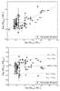 |
Fig. 11 Comparison of spectroscopic masses and evolutionary masses for the 66 sources that have Mevol constrained by bonnsai. The upper panel shows a one-to-one comparison; the lower panel shows the ratio of the masses. |
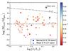 |
Fig. 12 Mass discrepancy plotted against luminosity for the 66 sources that have Mevol constrained by bonnsai. The upper dashed line is from the L(M) relation of helium stars; see main text for discussion. The lower line is Mspec = Mevol, and is a lower limit as stars cannot be under-luminous. The color denotes the surface helium abundance. Squares denote stars for which the LC is certain and triangles refer to the sources with weak Si iv relative to He i and for which the luminosity class may be debated (they may be dwarf stars). Helium enriched sources are all positioned above the one-to-one relation. |
The spectroscopic mass can be derived from the spectroscopically determined gravity and the K-band magnitude constrained radius. The gravities were corrected for the (small) contribution by the centrifugal acceleration (see Sect. 4.2). We derive the current evolutionary mass of our stars by comparison with the single-star evolutionary tracks of Brott et al. (2011) and Köhler et al. (2015). For this purpose, we used bonnsai2, a bayesian method, to constrain the evolutionary state of stars (Schneider et al. 2014). As independent prior functions, we adopt a Salpeter (1955) initial mass function, an initial rotational velocity distribution from Paper XII, a random orientation of rotation axes, and a uniform age distribution (equivalent to a past constant star-formation rate). As for the observables, we used the derived effective temperature, luminosity, and projected spin velocity. Because of the limited resolution of the model grid, we impose minimum error bars of 500 K in Teff and 0.1 dex in log L. On the basis of these constraints, we computed the posterior probability distribution of the present-day mass for each star, yielding its mean mass and associated 68% confidence intervals. The evolutionary tracks that were used are limited to the main-sequence, that is, evolved stars that are moving blueward in the HRD are not considered. In all cases (66 stars) the probability distribution of current evolutionary masses Mevol yielded a single, well defined peak. Both spectroscopic and evolutionary mass estimates are given in Table C.4.
The spectroscopic and evolutionary masses are compared in Fig. 11. For relatively small masses, the uncertainty in the spectroscopic mass is often larger than the uncertainty in the evolutionary mass. For the high-mass sources, the uncertainties in the evolutionary masses become larger as the observables span a larger mass range per unit temperature and luminosity. For the sample as a whole, we find a weighted mean in log (Mevol/Mspec) of 0.081 ± 0.009, that is, small but significant. However, the scatter is sizeable (1σ dispersion of 0.201 ± 0.010), which precludes confirmation of a systematic mass discrepancy.
Following earlier work (e.g., McEvoy et al. 2015), Fig. 12 shows the mass discrepancy, in terms of log (Mevol/Mspec), as a function of luminosity. According to stellar models, a He-enriched star of given mass is expected to be more luminous than its He-normal equivalent (Langer 1992), that is, yield a higher Mevol. This effect is illustrated by the upper dashed line in Fig. 12, which represents the mass discrepancy that could arise if the source were fitted with a baseline helium abundance Y = 0.255 while in reality it is a pure helium star (Y = 1.0), adopting the L(M) relation for helium stars of Gräfener et al. (2011). The He-enriched stars do seem to systematically show higher evolutionary masses than spectroscopic masses. However, we do not find a clear trend of the mass discrepancy with respect to the helium abundances of the stars.
It is interesting to note the subgroup of late O III and II stars in our sample (those that have weak Si iv features, see Sect. 4.2 of this paper and Tables A.1 and 2 in Walborn et al. (2014); labeled as triangles in Fig. 12). These sources systematically show larger spectroscopic than evolutionary masses (weighted mean log (Mevol/Mspec) = −0.148 ± 0.012), which is the opposite to what is usually reported in the literature (e.g., Herrero et al. 1992). Whether this is related to their nature remains unclear. We do note that they occupy a region in the HRD relatively devoid of O-dwarfs, which supports the hypothesis that they are regular main-sequence O-type stars (see Fig. 9 and the corresponding discussion in Sect. 4.4).
In view of the potential luminosity classification intricacy of the aforementioned group, we also assess the presence or lack of a discrepancy excluding these sources. Hence for the remaining stars (labelled as squares in Fig. 12), we find a weighted mean of log (Mevol/Mspec) = 0.106 ± 0.007. This suggests the presence of a modest (systematic) mass discrepancy for this subset. However, again, scatter is sizeable with a 1σ dispersion of 0.184 ± 0.007.
Again excluding the sources for which the luminosity class is debated (see above and Sect. 4.2) one might perceive by eye a trend similar to that reported by Trundle & Lennon (2005) and McEvoy et al. (2015). However, the Pearson correlation coefficient does not allow us to accept the presence of such a linear trend at the 5% significance level. We also computed the Spearman’s and Kendall’s rank correlations and reached the same conclusions that our data does not allow us to establish the significance of any trend between the degree of mass discrepancy (log (Mevol/Mspec)) and the stellar luminosity.
Finally, though certain individuals show worrying inconsistencies, the data does not allow us to confirm nor to reject the presence of a systematic mass discrepancy.
5. Summary
We have determined the stellar and wind properties of the 72 presumably single O-type giants, bright giants, and supergiants observed in the context of the VLT-FLAMES Tarantula Survey. Our main findings can be summarized as follows:
-
We use our sample of LMC stars and the sample analyzed byMokiem et al. (2007b) to calibratethe spectral type versus Teff dependence for luminosity class III and I in the spectral range O3-O9. Linear relations for these calibrations are provided in Table 1.
-
Supergiants appear to be more evolved than the other luminosity classes and are among the brightest objects featuring the lowest surface gravities. Stars initially more massive than 60 M⊙ show giant characteristics already relatively early on in their evolution. Bright giants with M ≳ 25 M⊙ do not constitute a conspicuous group intermediate to giants and supergiants in the sHRD and HRD but instead reside in a large area of these two diagrams, ranging from the dwarf (LC V) domain to the supergiants (LC I).
-
The group of late-O III and II stars with log gc in between 4.0 and 4.5 reside in a region relatively close to the ZAMS that seems devoid of late dwarf O stars. This could point to a spectral classification issue. Indeed, though the primary luminosity criterion (the He ii λ4686/He i λ4713 ratio) indicates a LC III or II, the secondary criterion (the ratio of Si iv to He i lines) is more in line with a LC IV or V classification.
-
The positions of the O giants to supergiants in the HRD do not point to a preferred age but rather seem indicative of a continuum of ages. The sub-populations centered on the associations NGC 2070 (excluding its core cluster R136, not covered by the VFTS) and NGC 2060 (6.7′ south-west of R136) do not show preferred ages either, neither relative to each other nor relative to the remaining field population.
-
The sample of presumed single stars contains a handful of helium enriched stars (five stars with Y > 0.30), which all have νesini ≤ 200kms-1, and unenriched helium stars that spin in excess of 300 kms-1. This is not in accordance with expectations of rotational mixing in main-sequence stars as computed by the evolutionary tracks of Brott et al. (2011) and Köhler et al. (2015). While it is very unlikely that these stars are post-RSGs, we cannot exclude the possibility that they are post-interaction binaries. For four out of the six stars spinning in excess of 300 kms-1, we find a helium content below the primordial value. We consider this to be a spurious result that may indicate a present-day binary nature of these systems.
-
The β parameter of the wind acceleration law cannot be reliably constrained with our data. Its value however significantly impacts the derived mass-loss rates. Adopting theoretical β values from Muijres et al. (2012) yields a log Dmom−log L/L⊙ relation that is shifted upwards by ~0.3 dex compared to earlier LMC results from Mokiem et al. (2007a). The latter results can be recovered if we treat the wind acceleration β as a free parameter. The log Dmom−log L/L⊙ relation that we obtained can be reconciled with the mass-loss predictions of Vink et al. (2001) if the wind is clumped with a clump volume filling factor fV ~ 1/8−1/6.
-
The current masses derived from the spectroscopic analysis are in fair agreement with those derived from a comparison with evolutionary tracks, though the scatter is sizeable. We do not detect a conspicuous systematic mass discrepancy.
The analysis presented here is part of a project that aims to establish the properties of the bulk of the hot massive stars in the Tarantula Nebula. The aim is to better constrain the physics governing their evolution, specifically the role of rotational mixing, mass loss, and binarity. In a follow-up study we use the results obtained here to study the efficiency of rotational mixing in O III−I stars in more detail, using the surface nitrogen abundances as a probe (Grin et al. 2017). Of all massive stars that feature strong winds, the wind-driving mechanism of the group of O III−I stars is thought to be best understood. However, even for these objects, the intricacies of accurately establishing their wind properties remain challenging. Here, this is exemplified by a discussion of the degeneracy of the wind acceleration β and the mass-loss rate Ṁ if only optical spectra are analyzed (see also e.g. Markova et al. 2004). Firm constraints on both parameters, as well as an independent measure of the clumping properties of the outflowing gas, can be obtained from far-ultraviolet spectra and we signal the need to obtain such spectra to further our understanding of the mass-loss mechanism of the most massive stars. Finally, an in-depth reassessment of the luminosity class assignment of the group of late-O giants and bright giants featuring Si iv lines that are weak relative to He i lines is warranted. This should establish whether or not these stars form a separate physical group.
2MASS filter response function are tabulated at http://www.ipac.caltech.edu/2mass/releases/allsky/doc /sec6_4a.tbl3.html
The bonnsai web-service is available at https://www.astro.uni-bonn.de/stars/bonnsai/
Acknowledgments
O.H.R.A. acknowledges funding from the European Union’s Horizon 2020 research and innovation programme under the Marie Skłodowska-Curie grant agreement No. 665593 awarded to the Science and Technology Facilities Council. N.J.G. is part of the International Max Planck Research School (IMPRS) for Astronomy and Astrophysics at the Universities of Bonn and Cologne. S.S.D. and A.H. acknowledge funding by the Spanish Ministry of Economy and Competitiveness (MINECO) under grants AYA2010-21697-C05- 04, Consolider-Ingenio 2010 CSD2006-00070, and Severo Ochoa SEV-2011- 0187, and by the Canary Islands Government under grant PID2010119. M.G. and F.N. acknowledge MINECO grants FIS2012-39162-C06-01, ESP2013-47809-C3-1-R and ESP2015-65597-C4-1-R. C.S.S. acknowledges support from the Joint Committee ESO-Government of Chile and DIDULS programme from Universidad de La Serena under grant DIDULS Regular PR16145. N.M. acknowledges the financial support of the Bulgarian NSF under grant DN08/1/13.12.2016.
References
- Abbott, D. C., & Lucy, L. B. 1985, ApJ, 288, 679 [NASA ADS] [CrossRef] [Google Scholar]
- Almeida, L. A., Sana, H., Taylor, W., et al. 2017, A&A, 598, A84 [NASA ADS] [CrossRef] [EDP Sciences] [Google Scholar]
- Asplund, M., Grevesse, N., & Sauval, A. J. 2005, in Cosmic Abundances as Records of Stellar Evolution and Nucleosynthesis, eds. T. G. Barnes, III & F. N. Bash, ASP Conf. Ser., 336, 25 [Google Scholar]
- Bestenlehner, J. M., Gräfener, G., Vink, J. S., et al. 2014, A&A, 570, A38 (Paper XVII) [NASA ADS] [CrossRef] [EDP Sciences] [Google Scholar]
- Beuther, H., Linz, H., & Henning, T. 2008, Massive Star Formation: Observations Confront Theory, ASP Conf. Ser., 387 [Google Scholar]
- Bouret, J.-C., Lanz, T., Heap, S., et al. 2003, in SF2A-2003: Semaine de l’Astrophysique Francaise, eds. F. Combes, D. Barret, T. Contini, & L. Pagani, 499 [Google Scholar]
- Bouret, J.-C., Lanz, T., & Hillier, D. J. 2005, A&A, 438, 301 [NASA ADS] [CrossRef] [EDP Sciences] [Google Scholar]
- Bouret, J.-C., Lanz, T., Martins, F., et al. 2013, A&A, 555, A1 [NASA ADS] [CrossRef] [EDP Sciences] [Google Scholar]
- Bromm, V., Yoshida, N., Hernquist, L., & McKee, C. F. 2009, Nature, 459, 49 [NASA ADS] [CrossRef] [PubMed] [Google Scholar]
- Brott, I., de Mink, S. E., Cantiello, M., et al. 2011, A&A, 530, A115 [NASA ADS] [CrossRef] [EDP Sciences] [Google Scholar]
- Campbell, M. A., Evans, C. J., Mackey, A. D., et al. 2010, MNRAS, 405, 421 [NASA ADS] [Google Scholar]
- Castro, N., Fossati, L., Langer, N., et al. 2014, A&A, 570, L13 [NASA ADS] [CrossRef] [EDP Sciences] [Google Scholar]
- Charbonneau, P. 1995, ApJS, 101, 309 [NASA ADS] [CrossRef] [Google Scholar]
- Cioni, M.-R. L. 2016, The Universe of Digital Sky Surveys, 42, 49 [NASA ADS] [Google Scholar]
- Clark, J. S., Bartlett, E. S., Broos, P. S., et al. 2015, A&A, 579, A131 [NASA ADS] [CrossRef] [EDP Sciences] [Google Scholar]
- Cohen, M., Wheaton, W. A., & Megeath, S. T. 2003, AJ, 126, 1090 [NASA ADS] [CrossRef] [Google Scholar]
- Crowther, P. A., Hillier, D. J., Evans, C. J., et al. 2002, ApJ, 579, 774 [NASA ADS] [CrossRef] [Google Scholar]
- de Koter, A., Heap, S. R., & Hubeny, I. 1997, ApJ, 477, 792 [Google Scholar]
- de Koter, A., Heap, S. R., & Hubeny, I. 1998, ApJ, 509, 879 [NASA ADS] [CrossRef] [Google Scholar]
- De Marchi, G., Paresce, F., Panagia, N., et al. 2011, ApJ, 739, 27 [NASA ADS] [CrossRef] [Google Scholar]
- de Mink, S. E., Langer, N., Izzard, R. G., Sana, H., & de Koter, A. 2013, ApJ, 764, 166 [NASA ADS] [CrossRef] [Google Scholar]
- de Mink, S. E., Sana, H., Langer, N., Izzard, R. G., & Schneider, F. R. N. 2014, ApJ, 782, 7 [NASA ADS] [CrossRef] [Google Scholar]
- Doran, E. I., Crowther, P. A., de Koter, A., et al. 2013, A&A, 558, A134 [NASA ADS] [CrossRef] [EDP Sciences] [Google Scholar]
- Dunstall, P. R., Dufton, P. L., Sana, H., et al. 2015, A&A, 580, A93 [NASA ADS] [CrossRef] [EDP Sciences] [Google Scholar]
- Ekström, S., Georgy, C., Eggenberger, P., et al. 2012, A&A, 537, A146 [NASA ADS] [CrossRef] [EDP Sciences] [Google Scholar]
- Evans, C. J., Walborn, N. R., Crowther, P. A., et al. 2010, ApJ, 715, L74 [NASA ADS] [CrossRef] [Google Scholar]
- Evans, C. J., Taylor, W. D., Hénault-Brunet, V., et al. 2011, A&A, 530, A108 (Paper I) [NASA ADS] [CrossRef] [EDP Sciences] [Google Scholar]
- Eversberg, T., Lépine, S., & Moffat, A. F. J. 1998, ApJ, 494, 799 [NASA ADS] [CrossRef] [Google Scholar]
- Fullerton, A. W., Massa, D. L., & Prinja, R. K. 2006, ApJ, 637, 1025 [NASA ADS] [CrossRef] [Google Scholar]
- Garcia, M., Herrero, A., Najarro, F., Lennon, D. J., & Alejandro Urbaneja, M. 2014, ApJ, 788, 64 [NASA ADS] [CrossRef] [Google Scholar]
- Gräfener, G., Vink, J. S., de Koter, A., & Langer, N. 2011, A&A, 535, A56 [NASA ADS] [CrossRef] [EDP Sciences] [Google Scholar]
- Gray, D. 1976, The Observation and Analysis of Stellar Photospheres, 3rd edn. (Cambridge University Press) [Google Scholar]
- Grin, N. J., Ramírez-Agudelo, O. H., de Koter, A., et al. 2017, A&A, 600, A82 [NASA ADS] [CrossRef] [EDP Sciences] [Google Scholar]
- Groenewegen, M. A. T., & Lamers, H. J. G. L. M. 1989, A&AS, 79, 359 [NASA ADS] [Google Scholar]
- Groh, J. H., Meynet, G., Ekström, S., & Georgy, C. 2014, A&A, 564, A30 [NASA ADS] [CrossRef] [EDP Sciences] [Google Scholar]
- Herrero, A., Kudritzki, R. P., Vilchez, J. M., et al. 1992, A&A, 261, 209 [NASA ADS] [Google Scholar]
- Hillier, D. J., & Miller, D. L. 1998, ApJ, 496, 407 [NASA ADS] [CrossRef] [Google Scholar]
- Hirano, S., Hosokawa, T., Yoshida, N., et al. 2014, ApJ, 781, 60 [NASA ADS] [CrossRef] [Google Scholar]
- Hirano, S., Hosokawa, T., Yoshida, N., Omukai, K., & Yorke, H. W. 2015, MNRAS, 448, 568 [NASA ADS] [CrossRef] [Google Scholar]
- Hubeny, I. 1988, Comp. Phys. Comm., 52, 103 [Google Scholar]
- Hubeny, I., & Lanz, T. 1995, ApJ, 439, 875 [Google Scholar]
- Köhler, K., Langer, N., de Koter, A., et al. 2015, A&A, 573, A71 [NASA ADS] [CrossRef] [EDP Sciences] [Google Scholar]
- Kudritzki, R.-P., & Puls, J. 2000, ARA&A, 38, 613 [NASA ADS] [CrossRef] [Google Scholar]
- Langer, N. 1992, A&A, 265, L17 [NASA ADS] [Google Scholar]
- Langer, N. 2012, ARA&A, 50, 107 [NASA ADS] [CrossRef] [Google Scholar]
- Langer, N., & Kudritzki, R. P. 2014, A&A, 564, A52 [NASA ADS] [CrossRef] [EDP Sciences] [Google Scholar]
- Lanz, T., & Hubeny, I. 2007, ApJS, 169, 83 [CrossRef] [Google Scholar]
- Leitherer, C., Robert, C., & Drissen, L. 1992, ApJ, 401, 596 [NASA ADS] [CrossRef] [Google Scholar]
- Lépine, S., & Moffat, A. F. J. 2008, AJ, 136, 548 [NASA ADS] [CrossRef] [Google Scholar]
- MaízApellániz, J., Sota, A., Arias, J. I., et al. 2016, ApJS, 224, 4 [NASA ADS] [CrossRef] [Google Scholar]
- Markova, N., Puls, J., Repolust, T., & Markov, H. 2004, A&A, 413, 693 [NASA ADS] [CrossRef] [EDP Sciences] [Google Scholar]
- Martins, F., Schaerer, D., & Hillier, D. J. 2005, A&A, 436, 1049 [NASA ADS] [CrossRef] [EDP Sciences] [Google Scholar]
- Massa, D., Fullerton, A. W., Sonneborn, G., & Hutchings, J. B. 2003, ApJ, 586, 996 [NASA ADS] [CrossRef] [Google Scholar]
- Massey, P., Bresolin, F., Kudritzki, R. P., Puls, J., & Pauldrach, A. W. A. 2004, ApJ, 608, 1001 [Google Scholar]
- Massey, P., Puls, J., Pauldrach, A. W. A., et al. 2005, ApJ, 627, 477 [NASA ADS] [CrossRef] [Google Scholar]
- Massey, P., Zangari, A. M., Morrell, N. I., et al. 2009, ApJ, 692, 618 [NASA ADS] [CrossRef] [Google Scholar]
- Massey, P., Neugent, K. F., Hillier, D. J., & Puls, J. 2013, ApJ, 768, 6 [NASA ADS] [CrossRef] [Google Scholar]
- Matteucci, F. 2008, in Massive Stars as Cosmic Engines, eds. F. Bresolin, P. A. Crowther, & J. Puls, IAU Symp., 250, 391 [Google Scholar]
- McEvoy, C. M., Dufton, P. L., Evans, C. J., et al. 2015, A&A, 575, A70 [NASA ADS] [CrossRef] [EDP Sciences] [Google Scholar]
- Meynet, G., & Maeder, A. 2005, A&A, 429, 581 [Google Scholar]
- Mokiem, M. R., de Koter, A., Puls, J., et al. 2005, A&A, 441, 711 [NASA ADS] [CrossRef] [EDP Sciences] [Google Scholar]
- Mokiem, M. R., de Koter, A., Evans, C. J., et al. 2006, A&A, 456, 1131 [NASA ADS] [CrossRef] [EDP Sciences] [Google Scholar]
- Mokiem, M. R., de Koter, A., Evans, C. J., et al. 2007a, A&A, 465, 1003 [NASA ADS] [CrossRef] [EDP Sciences] [Google Scholar]
- Mokiem, M. R., de Koter, A., Vink, J. S., et al. 2007b, A&A, 473, 603 [NASA ADS] [CrossRef] [EDP Sciences] [Google Scholar]
- Muijres, L. E., de Koter, A., Vink, J. S., et al. 2011, A&A, 526, A32 [Google Scholar]
- Muijres, L. E., Vink, J. S., de Koter, A., Müller, P. E., & Langer, N. 2012, A&A, 537, A37 [NASA ADS] [CrossRef] [EDP Sciences] [Google Scholar]
- Najarro, F., Hanson, M. M., & Puls, J. 2011, A&A, 535, A32 [NASA ADS] [CrossRef] [EDP Sciences] [Google Scholar]
- Oskinova, L. M., Hamann, W.-R., & Feldmeier, A. 2007, A&A, 476, 1331 [NASA ADS] [CrossRef] [EDP Sciences] [Google Scholar]
- Peimbert, M., Luridiana, V., & Peimbert, A. 2007, ApJ, 666, 636 [NASA ADS] [CrossRef] [Google Scholar]
- Pietrzyński, G., Graczyk, D., Gieren, W., et al. 2013, Nature, 495, 76 [NASA ADS] [CrossRef] [PubMed] [Google Scholar]
- Podsiadlowski, P., Joss, P. C., & Hsu, J. J. L. 1992, ApJ, 391, 246 [NASA ADS] [CrossRef] [Google Scholar]
- Prantzos, N. 2000, New Astron. Rev., 44, 303 [NASA ADS] [CrossRef] [Google Scholar]
- Prinja, R. K., & Massa, D. L. 2010, A&A, 521, L55 [Google Scholar]
- Puls, J., Kudritzki, R.-P., Herrero, A., et al. 1996, A&A, 305, 171 [NASA ADS] [Google Scholar]
- Puls, J., Springmann, U., & Lennon, M. 2000, A&ARv, 141, 23 [Google Scholar]
- Puls, J., Urbaneja, M. A., Venero, R., et al. 2005, A&A, 435, 669 [NASA ADS] [CrossRef] [EDP Sciences] [Google Scholar]
- Puls, J., Vink, J. S., & Najarro, F. 2008, A&ARv, 16, 209 [NASA ADS] [CrossRef] [EDP Sciences] [Google Scholar]
- Ramírez-Agudelo, O. H., Simón-Díaz, S., Sana, H., et al. 2013, A&A, 560, A29 (Paper XII) [NASA ADS] [CrossRef] [EDP Sciences] [Google Scholar]
- Ramírez-Agudelo, O. H., Sana, H., de Mink, S. E., et al. 2015, A&A, 580, A92 [NASA ADS] [CrossRef] [EDP Sciences] [Google Scholar]
- Repolust, T., Puls, J., & Herrero, A. 2004, A&A, 415, 349 [NASA ADS] [CrossRef] [EDP Sciences] [Google Scholar]
- Rivero González, J. G., Puls, J., & Najarro, F. 2011, A&A, 536, A58 [NASA ADS] [CrossRef] [EDP Sciences] [Google Scholar]
- Rivero González, J. G., Puls, J., Massey, P., & Najarro, F. 2012a, A&A, 543, A95 [NASA ADS] [CrossRef] [EDP Sciences] [Google Scholar]
- Rivero González, J. G., Puls, J., Najarro, F., & Brott, I. 2012b, A&A, 537, A79 [NASA ADS] [CrossRef] [EDP Sciences] [Google Scholar]
- Rolleston, W. R. J., Trundle, C., & Dufton, P. L. 2002, A&A, 396, 53 [NASA ADS] [CrossRef] [EDP Sciences] [Google Scholar]
- Rubele, S., Kerber, L., Girardi, L., et al. 2012, A&A, 537, A106 [NASA ADS] [CrossRef] [EDP Sciences] [Google Scholar]
- Sabbi, E., Lennon, D. J., Anderson, J., et al. 2016, ApJS, 222, 11 [NASA ADS] [CrossRef] [Google Scholar]
- Sabín-Sanjulián, C., Simón-Díaz, S., Herrero, A., et al. 2014, A&A, 564, A39 (Paper XIII) [NASA ADS] [CrossRef] [EDP Sciences] [Google Scholar]
- Sabín-Sanjulián, C., Simón-Díaz, S., Herrero, A., et al. 2017, A&A, in press DOI: 10.1051/0004-6361/201629210 [Google Scholar]
- Salpeter, E. E. 1955, ApJ, 121, 161 [Google Scholar]
- Sana, H., Rauw, G., & Gosset, E. 2001, A&A, 370, 121 [NASA ADS] [CrossRef] [EDP Sciences] [Google Scholar]
- Sana, H., de Koter, A., de Mink, S. E., et al. 2013, A&A, 550, A107 [NASA ADS] [CrossRef] [EDP Sciences] [Google Scholar]
- Schneider, F. R. N., Langer, N., de Koter, A., et al. 2014, A&A, 570, A66 [Google Scholar]
- Seaton, M. J. 1958, MNRAS, 118, 504 [NASA ADS] [CrossRef] [Google Scholar]
- Simón-Díaz, S., Caballero, J. A., & Lorenzo, J. 2011, ApJ, 742, 55 [NASA ADS] [CrossRef] [Google Scholar]
- Simón-Díaz, S., Herrero, A., Sabín-Sanjulián, C., et al. 2014, A&A, 570, L6 [NASA ADS] [CrossRef] [EDP Sciences] [Google Scholar]
- Simón-Díaz, S., Caballero, J. A., Lorenzo, J., et al. 2015, ApJ, 799, 169 [NASA ADS] [CrossRef] [Google Scholar]
- Sota, A., Maíz Apellániz, J., Walborn, N. R., et al. 2011, ApJS, 193, 24 [NASA ADS] [CrossRef] [Google Scholar]
- Sota, A., Maíz Apellániz, J., Morrell, N. I., et al. 2014, ApJS, 211, 10 [NASA ADS] [CrossRef] [Google Scholar]
- Sundqvist, J. O., Puls, J., & Feldmeier, A. 2010, A&A, 510, A11 [NASA ADS] [CrossRef] [EDP Sciences] [Google Scholar]
- Sundqvist, J. O., Puls, J., Feldmeier, A., & Owocki, S. P. 2011, A&A, 528, A64 [NASA ADS] [CrossRef] [EDP Sciences] [Google Scholar]
- Sundqvist, J. O., Puls, J., & Owocki, S. P. 2014, A&A, 568, A59 [NASA ADS] [CrossRef] [EDP Sciences] [Google Scholar]
- Šurlan, B., Hamann, W.-R., Aret, A., et al. 2013, A&A, 559, A130 [NASA ADS] [CrossRef] [EDP Sciences] [Google Scholar]
- Tramper, F., Sana, H., de Koter, A., & Kaper, L. 2011, ApJ, 741, L8 [NASA ADS] [CrossRef] [Google Scholar]
- Tramper, F., Sana, H., de Koter, A., Kaper, L., & Ramírez-Agudelo, O. H. 2014, A&A, 572, A36 [NASA ADS] [CrossRef] [EDP Sciences] [Google Scholar]
- Trundle, C., & Lennon, D. J. 2005, A&A, 434, 677 [Google Scholar]
- Trundle, C., Lennon, D. J., Puls, J., & Dufton, P. L. 2004, A&A, 417, 217 [NASA ADS] [CrossRef] [EDP Sciences] [Google Scholar]
- Vink, J. S., & Gräfener, G. 2012, ApJ, 751, L34 [NASA ADS] [CrossRef] [Google Scholar]
- Vink, J. S., de Koter, A., & Lamers, H. J. G. L. M. 1999, A&A, 350, 181 [NASA ADS] [Google Scholar]
- Vink, J. S., de Koter, A., & Lamers, H. J. G. L. M. 2001, A&A, 369, 574 [NASA ADS] [CrossRef] [EDP Sciences] [Google Scholar]
- Vink, J. S., Brott, I., Gräfener, G., et al. 2010, A&A, 512, L7 [NASA ADS] [CrossRef] [EDP Sciences] [Google Scholar]
- Walborn, N. R. 1973, AJ, 78, 1067 [NASA ADS] [CrossRef] [Google Scholar]
- Walborn, N. R., & Blades, J. C. 1997, ApJS, 112, 457 [NASA ADS] [CrossRef] [Google Scholar]
- Walborn, N. R., Sana, H., Simón-Díaz, S., et al. 2014, A&A, 564, A40 [NASA ADS] [CrossRef] [EDP Sciences] [Google Scholar]
- Zhang, B., Zhang, B.-B., Virgili, F. J., et al. 2009, ApJ, 703, 1696 [NASA ADS] [CrossRef] [Google Scholar]
Appendix A: Projected rotational velocity ve sin i
Paper XII presents the rotational properties of the spectroscopic single O-type stars by taking into account line broadening due to macro-turbulent motions. The stars analyzed in this paper are a subset of those analyzed in Paper XII. Here we determine νesini neglecting macro-turbulent motions. Our results may, therefore, differ from Paper XII.
Figure A.1 shows a comparison of both νesini estimates using different representations of the difference. The systematic difference of all stars in common is approximately 7 kms-1 with a standard deviation 21 kms-1. This is in agreement with the uncertainties discussed in Paper XII. Qualitatively, the shape of the (cumulative) νesini distribution is similar in both methodologies (see upper and middle panels). Below 160 kms-1, the values presented here tend to somewhat overestimate νesini. This is a consequence of not distinguishing between broadening from rotation and macro turbulence in the regime where rotation does not dominate the line width. Hence, the νesini values up to 160 kms-1 derived here may be overestimated by up to several tens of kms-1. Such overestimates do not, however, impact the determination of other stellar properties in any significant way.
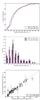 |
Fig. A.1 Cumulative (upper panel) and frequency (middle panel) distributions of the projected rotational velocities of the O-type LC III to I as derived here from the automated fastwind analysis and Paper XII. The middle panel shows Poissonian error bars. The lower panel compares the actual νesini of these two samples. |
Appendix B: HRD as a function of the spatial location in 30 Dor
In Sect. 4.4, we investigated the evolutionary status of our sample stars by placing them in the Hertzsprung-Russell diagram. Fig. B.1 shows HRDs of sub-populations selected with respect to their spatial location: NGC 2070 (upper panel), NGC 2060 (middle panel) and stars outside the two star-forming complexes (lower panel), all complemented with the VFTS dwarfs and VMS stars. As pointed out, stars of LC III to I are, on average, more evolved than the LC V. Stars in R136 are not resolved spatially with VLT-FLAMES and are therefore omitted from our sample. Though it is likely that the stars in R136 are younger, no apparent age differences are present in the three populations specified here: they all show an age spread between approximately 2 and 5 Myr.
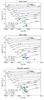 |
Fig. B.1 Hertzsprung-Russell diagram of the sample as a function of spatial location: NGC 2070 (upper panel), NGC 2060 (middle panel) and stars outside star-forming complexes (lower panel). Evolutionary tracks (solid lines) and isochrones (dot-dashed lines) are from stellar models initially rotating with approximately 200 kms-1 (Brott et al. 2011; Köhler et al. 2015). |
Appendix C: Additionnal tables
List of the diagnostic lines for the O giants, bright giants, and supergiants for which hydrogen, helium, and nitrogen have been included and used simultaneously in the determination of the stellar and wind parameters.
List of the H and He diagnostic lines included in the analysis of the O giants, bright giants, and supergiants.
List of the H and He diagnostic lines included in the analysis of O stars without luminosity class.
Best-fitting atmospheric and wind parameters of our sample stars.
Best-fitting atmospheric and wind parameters of the stars with no luminosity class.
Appendix D: Special remarks on the fitted stars
This section presents notes on the fitting results of some of the sample stars as well as additional remarks on peculiar properties of the objects that are presented in Appendix E. Some stars from our presumably single-star sample were part of the Tarantula Massive Binary Monitoring (TMBM), a 32-epoch radial velocity program that followed up on VFTS RV variable stars (Almeida et al. 2017). In those cases, results are also included. Details on the spectral classification are included in Tables A.1 and A.2 of Walborn et al. (2014) and hence are not repeated here.
-
VFTS 046 is one of the helium-enriched stars. The cores of the Balmer lines are clipped because of remaining residuals of nebular contamination. The best models overpredict He iλ4387 by 5% with respect to the continuum. The rest of the line profiles are very well reproduced (rms better than 1% of the continuum).
-
VFTS 064 (SB1). The cores of the Balmer lines are clipped because of remaining residuals of nebular contamination. Except for He iiλ4686, the lines are well fitted (rms better than 1% of the continuum). The data of He iiλ4686 are red-shifted by ~2 Å compared to the models. TMBM has identified the star as a single-lined (SB1) spectroscopic binary with a tentative period of approximately 900 d. Its binary nature is likely the cause of the He iiλ4686 discrepancy. This star is excluded from the analysis in Sect. 4.
-
VFTS 087’s Hα observed profile is not used because it presents strong nebular emission. The cores of Hβ−γ are clipped because of remaining residuals of nebular contamination. Its spectrum also shows strong nitrogen lines (i.e., N iiλ3995, N iiiλ4097, 4195, 4379, 4511, 4515, 4518, 4523) and hence they are taken into account for the fit. Most of the lines are well fitted (rms better than 1% of the continuum) except for He iiλ4686. The data of He iiλ4686 are slightly red-shifted by ~0.2 Å compared to the models. Further, the star shows a significant but moderate RV variability with a peak-to-peak amplitude of approximately 12 kms-1. It was followed up by TMBM but no periodicity was found.
-
VFTS 103’s Balmer line cores and He iλ4713, 4922 cores are clipped because of remaining residuals of nebular contamination. The models overpredict He iiλ4200, 4541 by 3% and 2% with respect to the continuum, respectively. For the remaining lines the differences are less than 1% (with respect to the continuum). He iiλ4686 shows a tentative structure, possibly reminiscent of a blended profile.
-
VFTS 104’s VISTA K-band measurement is not available. We have adopted the K magnitude from the InfraRed Survey Facility (IRSF; see also Table 6 of Paper I). The cores of the Balmer lines are clipped because of residuals of nebular contamination. The models fairly reproduce the line depths and widths of the spectral lines.
-
VFTS 113’s Balmer line cores are clipped because of significant nebular correction residuals. The models reproduce the spectral lines well. The star was followed up by TMBM but no periodicity was found despite a rather large peak-to-peak RV variability of 28 kms-1.
-
VFTS 141’s Balmer line cores are clipped. The models underpredict He iiλ4200, 4541 by ~2% with respect to the continuum, possibly indicating that the temperature has been underestimated. The remaining lines are all well reproduced by the model (rms better than 1%).
-
VFTS 151’s Hα observed profile is not used because it presents strong emission. The cores of Hβ−γ are clipped because of remaining residuals of nebular contamination. The best models overpredict He iλ4387 by 3% with respect to the continuum and fail to reproduce the wings of He iλ4471 and the red wing of He iiλ4686. The remaining lines are well reproduced by the models and hence this star is included in the analysis of Sect. 4 as an acceptable fit.
-
VFTS 153’s Balmer line cores are clipped. The best models overpredict He iiλ4200 by 2% with respect to the continuum and fail to reproduce the left wing of He iiλ4686. For the remaining lines, the models fairly reproduce the spectral lines (rms better than 1% of the continuum) and hence this star is included in the analysis of Sect. 4 as an acceptable fit.
-
VFTS 160’s Hα−β−γ and He iλ4387, 4713, 4922 cores are clipped. The models fail to reproduce the line depth and width of He iλ4387. For the remaining lines, the models (within the 95% confidence interval) acceptably reproduce the spectral lines and hence this star is included in the analysis of Sect. 4.
-
VFTS 171 (SB1). The cores of the Balmer lines are clipped. The observed profile of He iλ4026 and the wings of the Balmer lines are well fitted by the model. The data of He iiλ4686 are red-shifted by ~0.5 Å compared to the best model. For the remaining lines, the model presents incoherent line depths and widths. The differences are approximately 3% with respect to the continuum. VFTS 171 has been dentified by TMBM as a 670-d SB1 object. Hence this star is excluded from the analysis in Sect. 4.
-
VFTS 178’s Hα observed profile is not used because it presents strong nebular emission. The core of Hβ is clipped because of remaining residuals of nebular contamination. Its spectrum also shows strong nitrogen lines (i.e., N iiλ3995, N iiiλ4097, 4195, 4379, 4511, 4515, 4518, 4523) and hence they are taken into account for the fit. Most of the lines are well fitted (rms better than 1% of the continuum). VFTS 178 was also followed up by TMBM but no periodicity was found (ΔRV = 15kms-1).
-
VFTS 180 is one of the helium enriched stars. The He iλ4471, 4713 and Hα observed profiles are not used due to strong residuals of nebular contamination. The cores of the remaining Balmer lines are also clipped. Its spectrum shows strong nitrogen lines (i.e, N iiiλ4511, 4515, 4518, 4630, 4640, N ivλ4058) and hence they are taken into account for the fit. The data of N ivλ4058 are red-shifted by ~1 Å compared to the models. The remaining lines are fairly well reproduced by the models (rms better than 1% of the continuum), including the rather strong He iiλ4686 emission line, which is typical for strong stellar winds.
-
VFTS 192’s Balmer line cores are clipped. The lines are well fitted (rms of the order of 1% of the continuum), except for He iλ4471, although the latter differences probably result from a poor nebular correction in the observed data of that line. Finally, the He iiλ4686 spectral line seems slightly blue-shifted with respect to the best fit-model (~0.2 Å) but it is within the 95% probability models. While this may indicate a binary nature, the best fit model is still representative of the observed data.
-
VFTS 244’s Balmer line cores are clipped. The fit quality of the models is acceptable, with the exception of the He iiλ4686 line. The latter displays a small P-Cygni shape, with an absorption component that is significantly red-shifted (by ~1 Å) with respect to the model.
-
VFTS 253’s Hα−β−γ cores are clipped. The fit quality of the models is acceptable, though the He i line core seems narrower than the best-fit models but their wings are broader. This may indicate a composite nature or a significant macro-turbulent component (not included in our fitting approach).
-
VFTS 259’s Hα observed profile is not used in the fit because of strong residuals of nebular contamination. The cores of Hβ−γ are also clipped. For the fit, we have also used N iiiλ4634, 4640. The observed profile of He iiλ4686 is blue-shifted by 1 Å with respect to the best fit model. The remaining lines are well reproduced by the 95% models. The star displays RV variation amplitude of ΔRV = 23kms-1 according to TMBM. While a periodicity of 3.7 d was identified, the folded RV-curve does not resemble that of a spectroscopic binary system, suggesting another origin for the line variability. Hence VFTS 259 is included in the analysis of Sect. 4.
-
VFTS 267’s Balmer line and He iλ4471 cores are clipped because of remaining residuals of nebular contamination. The observed profiles of the He i lines are relatively weak suggesting a very hot star. The N ivλ4058, and N vλ4603, 4619 lines are thus included in the fitting. The He iλ4026, He iiλ4200, 4541 and the wings of Hδ−γ−β are fairly well fitted by the best models. He iiλ4686 and Hα show P-cygni profiles, though He iiλ4686 is peculiar with an apparent excess absorption on top of the P-cygni profile. The model reproduces the red wings of these two lines and N ivλ4058, and N vλ4603, 4619 within 2% with respect to the continuum. The data of the nitrogen lines are slightly red-shifted (0.5 Å) with respect to the best model. TMBM identified a significant ΔRV of 22 kms-1 but no periodicity.
-
VFTS 306’s Balmer line cores are are clipped. The He iiλ4686 line profile is red-shifted by ~1 Å compared to the best model. For the remaining lines, the fit quality of the 95% probability models is acceptable (rms of 1% with respect to the continuum).
-
VFTS 332 (SB1). The cores of the Balmer lines are clipped because of remaining residuals of nebular contamination. Only He iλ4026 and the wings of Hδ−γ−β are well fitted. The data of He iiλ4686 is red-shifted by ~0.5 Å compared to the model. For the remaining lines, models within our 95% confidence interval manage to reproduce most of the profile properties. TMBM results however revealed it is a long orbital period (P ~ 3 yr) binary.
-
VFTS 333 (SB1). The cores of the Balmer lines are clipped because of remaining residuals of nebular contamination. The data of He iiλ4686 is red-shifted by ~1.0 Å compared to the model. For the remaining lines, models within our 95% confidence interval manage to reproduce most of the profile properties. TMBM results however revealed a binary nature with a period of P ~ 3 yr.
-
VFTS 370’s Balmer line cores and the red wing of He iλ4471 are clipped because of remaining residuals of nebular contamination. The He iλ4026, left wing of He iλ4471 and the wings of the Balmer lines are well fitted (rms better than 1% of the continuum). The model underpredicts He iiλ4200, 4541 by 1% with respect to the continuum. For the remaining lines, the line depths (widths) are slightly underestimated (overestimated). The differences are, however, small (<2% with respect to the continuum) and seemingly within the range of models that meet our 95%-confidence criteria.
-
VFTS 399’s Hα observed profile is not used because it presents strong emission. Cores of the remaining Balmer and He iλ4471 lines are clipped because of residuals of nebular contamination. The model underpredicts He iλ4200, 4541, and 4686 by 2% with respect to the continuum. The remaining lines are well fitted by the model (rms better that 1% with respect to the continuum). VFTS 399 was identified as an X-ray binary by Clark et al. (2015).
-
VFTS 440 (SB1). The cores of the Balmer lines are clipped because of remaining residuals of nebular contamination. The observed profile of He iiλ4686 presents an inverse P-cygni profile, of which the absorption is red-shifted by 2 Å compared to the best-fit model. The model fails to reproduce the line depths and widths of all lines. Hence this star is excluded from further analysis in Sect. 4. TMBM result indicate that it is a P ~ 100 d binary, providing an explanation for the shift in the He iiλ4686 spectral line. In such a scenario, the peculiar He iiλ4686 profile may resuls from an isothermal wind-wind collision zone, as in the case of, HD 152248 (Sana et al. 2001), for example.
-
VFTS 466’s Balmer line cores are clipped. The He iλ4026 and the wings of the Balmer lines are well fitted by the model (rms better than 1% of the continuum). The data of He iλ4471 present an asymmetry in the core and hence it is not well reproduced by the model; such core-infilling may result from limited nebular correction quality. The lines He iλ4713 and He iiλ4200 are underpredicted by 2% with respect to the continuum by the best-fit models, but some models within the 95%-confidence interval better reproduce these lines. The remaining lines are all well fitted by the model (rms better than 1% of the continuum).
-
VFTS 502’s Balmer line and He iλ4471, and 4922 cores are clipped because of remaining residuals of nebular contamination. The fit quality of the models is acceptable, with the exception of the right wing of Hγ and He iiλ4686. The former presents a blend that is not reproduced by the models. The latter is slightly red-shifted with respect to the best-fit model (~0.5 Å) but it is within the 95% probability models.
-
VFTS 503’s K-band magnitude from VISTA is not available, thus we have adopted the K magnitude from VLT-MAD observations of Campbell et al. (2010). The cores of the Balmer and He iλ4026, 4471, and 4922 lines are clipped because of remaining residuals of nebular contamination. The fit quality of the models is acceptable. The data of He iiλ4686 are slightly red-shifted with respect to the best-fit model (~0.5 Å) but still it is within the 95% probability models.
-
VFTS 513’s He iλ4713 and Hα observed profiles are not used because of contamination from strong emission. Large part of the cores of the remaining Balmer and He i lines are clipped. The Hδ and He iiλ4200 lines are well fitted (rms better than 1% of the continuum). The fit quality of the models for the remaining lines is acceptable, with the exception of the He iiλ4686 line. The latter is red-shifted with respect to the best-fit model by ~1.0 Å but it is within the 95% probability models.
-
VFTS 518 is one of the helium enriched stars. The cores of the Balmer and He iλ4026, 4471 are clipped. The data of the He i lines are relatively weak, thus the data of N iiiλ4634, 4640, 4641, N ivλ4058, and N vλ4603, 4619 are included. Despite that the data of He iiλ4686 and N ivλ4058 are slightly red-shifted with respect to the best-fit model (<0.3 Å), the model reproduces the depths and widths of the spectral lines (rms approximately 1% of the continuum).
-
VFTS 546’s Balmer line and He i line cores are widely clipped because of residuals of nebular contamination. Except for the left wing of He iλ4922, the model well reproduces the data of He iiλ4200, 4541, and 4686 and the wings of the remaining lines (rms of 1% of the continuum).
-
VFTS 566’s Balmer line and He i line cores are clipped because of residuals of nebular contamination. The data of the He i lines are relatively weak, thus the data of N iiiλ4634, 4640, 4641, N ivλ4058, and N vλ4603, 4619 are included. Though the data of He iiλ4686 and the nitrogen lines are slightly red-shifted with respect to the model (<0.5 Å), the model reproduces the depths and widths of the lines relatively well (rms approximately 1% of the continuum).
-
VFTS 569’s data of Hα and He iλ4713 are not used because of contamination from strong nebular emission. The cores of Balmer and He i lines are widely clipped. The models reproduce the profiles of He iiλ4200, 4541, and 4686 and the wings of the remaining lines (rms of 1% of the continuum).
-
VFTS 571’s K-band magnitude from VISTA is not available, thus we have adopted the K-band magnitude from VLT-MAD observations of Campbell et al. (2010). The cores of the Balmer and He i lines are clipped because of remaining nebular contamination. Best model underpredicts He iiλ4200, 4541 by 4% with respect to the continuum. The other diagnostic lines are strong and are relatively well reproduced by the model (rms of 1% of the continuum).
-
VFTS 599’s Balmer line and He iλ4387, 4471 cores are clipped. The data of the He i lines are relatively weak, thus the data of N iiiλ4634, 4640, 4641, N ivλ4058, and N vλ4603, 4619 are included. The data of He iiλ4686 and the nitrogen lines are slightly red-shifted with respect to the best-fit model (<0.5 Å), the model relatively well reproduces the depths and widths of the other lines (rms approximately 1% of the continuum), despite an incomplete sampling of the parameter space.
-
VFTS 620’s K-band magnitude from VISTA is not available, thus we have adopted the K-band magnitude from VLT-MAD observations of Campbell et al. (2010). The observed profile of Hα is not considered because of contamination of strong nebular emission. The cores of the Balmer lines are clipped because of residual nebular contamination. The model fairly reproduces the remaining diagnostic lines (rms better than1% of the continuum).
-
VFTS 664’s Balmer line cores are clipped because of remaining residuals of nebular contamination. The He iλ4026 and He iiλ4541 lines are well fitted by the best model (rms of 1% of the continuum). For the remaining lines, the fit quality of the models are acceptable, except that they tend to over predict the full width at half maximum (FWHM) (hence probably the rotation rate as well) of the He i lines.
-
VFTS 669’s Hα observed profile is not used because it presents strong nebular emission. The cores of Hβ−γ are clipped because of remaining residuals of nebular contamination. To fit its spectrum we also used nitrogen lines (i.e, N iiλ3995, N iiiλ4097, 4195, 4379, 4511, 4515, 4518, 4523). Most of the lines are well fitted (rms better than 1% of the continuum) except for He iiλ4686. The data of He iiλ4686 was 2% re-normalized with respect to the continuum.
-
VFTS 711’s Balmer line and He iλ4471 cores are clipped. Given the quality of the spectrum, we have fixed the νesini to the value obtained in Paper XII (νesini = 39 kms-1). The He iiλ4200, 4541 and the Balmer wings are well fitted by the best model (rms of 1% of the continuum). For the remaining lines, the fit quality of the models is acceptable.
-
VFTS 764’s Hα observed profile is not used because it presents strong nebular emission. The data of the He ii lines are relatively weak, the following nitrogen lines: N iiλ3995, N iiiλ4097, 4195, 4379, 4511, 4515, 4518, 4523 are included in the analysis. The fit quality of the models is acceptable, with the exception of N iiλ3995, Hβ and He iiλ4686. TMBM revealed a RV variability with a ΔRV of 27 kms-1. The data are compatible with a periodicity of 1.2 d though the folded RV-curve does not support a binary nature.
-
VFTS 777’s Balmer line and He iλ4471 cores are clipped. The fit best-fit model is acceptable, with the exception of the right wing of Hδ. The latter presents a blend that is not reproduced by the models.
Stars without luminosity classes
Here we also provide stellar parameters of VFTS stars for which no LC classification could be assigned (see Walborn et al. 2014). Most of these stars present low S/N, strong residuals of the nebular correction, or both. The Balmer and He i lines are often widely clipped. In a number of cases, the He i information (width, amplitude) is almost entirely lost. Nevertheless, we comment here on our results in case they are useful for follow up investigations.
-
VFTS 051’s Hα observed profile is not used because it presents strong emission. Given the quality of the spectrum, we have fixed the νesini to the value obtained in Paper XII (νesini = 412 kms-1). For the remaining Balmer lines, the cores are widely clipped because of remaining residuals of nebular contamination. The model well reproduces the wings of the Balmer lines. The shallow and noisy He i+ii spectral lines do not add much information and hence the stellar parameters are poorly constrained.
-
VFTS 125’s Balmer line cores are widely clipped. The observed profiles of the He i lines are relatively weak suggesting a very hot star. The N iiiλ4634, 4640, 4641 N ivλ4058, and N vλ4603, 4619 line profiles are thus included in the fitting. The model reproduces He iiλ4200, 4541 and the wings of Hβ−γ−δ. Given the significant noise in the spectral lines, the stellar parameters present sizeable error bars.
-
VFTS 145 is rated as a poor-quality fit. The observed profile of He iiλ4686 is not used because it has a suspicious normalization. The cores of Hα−β lines were clipped. Except for He i+iiλ4026, the model fails to reproduce the line depths and widths of the observed lines. The differences vary between 2% (He iλ4713) and 5% (Hγ) with respect to the continuum.
-
VFTS 360 is rated as a poor-quality fit. The observed profiles of Hα−β are not used because they present strong emission. The parameter space is deficiently explored and hence the model fails to reproduce line depths and widths of the most of the observed lines.
-
VFTS 373’s Balmer line and He iλ4026, 4387, 4471 cores are clipped. Except for He iλ4387, 4471, the model reproduces the observed diagnostic lines. The differences are of 1% with respect to the continuum.
-
VFTS 400 is rated as a poor-quality fit. The observed profile of Hα is not used because it presents strong emission. The cores of the remaining Balmer lines are clipped. Except for Hγ, the model fails to reproduce the line depths and widths of the observed lines. The differences vary between 2% (He iiλ4541) and 10% (He iλ4922).
-
VFTS 412’s Hα and He iλ4713 observed profiles are not used because they present strong emission. The cores of the remaining Balmer lines and He iλ4471, 4922 are clipped. The models overpredict the FWHM (hence likely the rotation) of all He i lines and under-predict their amplitudes.
-
VFTS 444’s Hα observed profile is not used because it presents strong emission. The cores of the remaining Balmer lines are clipped. The core of He iiλ4541 is also removed because of a strong absorption. Except for He iiλ4200, the model well reproduces the line depths and widths of the observed profiles (rms of 1% with respect to the continuum).
-
VFTS 446 is rated as a poor-quality fit. The observed profiles of Hα−β and He iλ4922 are not used because they present strong emission. The cores of Hγ−δ and He iλ4026, 4387, 4471 are widely clipped. Because the model can only rely on the He ii lines, the parameters are poorly constrained.
-
VFTS 451 is rated as a poor-quality fit. The cores of the Balmer lines and He iλ4387, 4471 are widely clipped because of remaining residuals of nebular contamination. The data of He iiλ4686 are red-shifted by 2 Å compared to the model. Except for He iiλ4200, 4541 the model has little information from the remaining observed lines and hence parameters are poorly constrained.
-
VFTS 456’s Hα and He iλ4713 observed profiles are not used because of strong emission. The cores of Hβ−γ−δ, He iλ4387, 4471 are clipped. For the remaining lines, the model reproduces the observed profiles with 1% with respect to the continuum.
-
VFTS 477’s Hα and He iλ4713 observed profiles are not used because of strong emission. The cores of Hβ−γ−δ and He iλ4387, 4471, and 4922 are widely clipped. As a result, almost no information is provided by the He i lines. The observed profile of He iiλ4686 is slightly red-shifted with respect to the model (0.5 Å), but in acceptable agrement given the large errors.
-
VFTS 515’s Hα and He iλ4713 observed profiles are not used because they present strong emission. The cores of Hβ−γ−δ and He iλ4387, 4471, 4922 are widely clipped; most of the information provided by He i is lost. The model slightly underestimates He iiλ4200, 4541 but failed to reproduce He iiλ4686 (no clear P-Cygni profile seen in the data). The estimated mass-loss rate is probably overestimated.
-
VFTS 519’s Hα, He iλ4713 and He iiλ4686 observed profiles are not used because of strong emission. Except for Hγ−δ and He iiλ4200, the observed profiles present a wrong normalization (i.e., continuum shifted by 5% with respect to the continuum).
-
VFTS 565 is rated as a poor-quality fit. The observed profile of Hα is not used because it presents strong emission. The cores of the Balmer lines and He iλ4387, 4713, 4922 are clipped. The data of He iλ4387, 4471 are red-shifted by 1 Å while He iiλ4686 is blue-shifted by 2 Å compared to the best model. Therefore, the observed profiles are poorly fitted.
-
VFTS 594. The observed profiles of Hα and He iλ4713 are not used because of strong emission. The cores of Hβ−γ−δ and He i lines are widely clipped. The models reproduce He iiλ4200, 4541 and the wings of the Balmer and He i lines. The data of He iiλ4686 are slightly red-shifted (0.3 Å) compared to the model.
Appendix E: Fitting results
In this appendix we show the spectra and the model fits for all our targets. We first show the results for the LC III to I stars (72 stars) and then we proceed with the stars without LCs (31 stars).
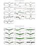 |
Fig. E.1 Observed spectra, the 95% probability models (green) and the best fit model (red) for VFTS 016 and 035. The vertical dashed lines indicate the wavelength range used to fit the corresponding diagnostic line. |
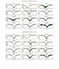 |
Fig. E.2 Observed spectra, the 95% probability models (green) and the best fit model (red) for VFTS 046 and 064. The vertical dashed lines indicate the wavelength range used to fit the corresponding diagnostic line. |
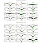 |
Fig. E.3 Observed spectra, the 95% probability models (green) and the best fit model (red) for VFTS 070 and 076. The vertical dashed lines indicate the wavelength range used to fit the corresponding diagnostic line. |
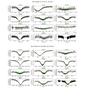 |
Fig. E.4 Observed spectra, the 95% probability models (green) and the best fit model (red) for VFTS 077 and 080. The vertical dashed lines indicate the wavelength range used to fit the corresponding diagnostic line. |
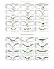 |
Fig. E.5 Observed spectra, the 95% probability models (green) and the best fit model (red) for VFTS 087 and 091. The vertical dashed lines indicate the wavelength range used to fit the corresponding diagnostic line. |
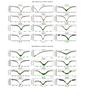 |
Fig. E.6 Observed spectra, the 95% probability models (green) and the best fit model (red) for VFTS 093 and 103. The vertical dashed lines indicate the wavelength range used to fit the corresponding diagnostic line. |
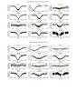 |
Fig. E.7 Observed spectra, the 95% probability models (green) and the best fit model (red) for VFTS 104 and 109. The vertical dashed lines indicate the wavelength range used to fit the corresponding diagnostic line. |
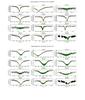 |
Fig. E.8 Observed spectra, the 95% probability models (green) and the best fit model (red) for VFTS 113 and 128. The vertical dashed lines indicate the wavelength range used to fit the corresponding diagnostic line. |
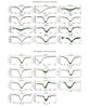 |
Fig. E.9 Observed spectra, the 95% probability models (green) and the best fit model (red) for VFTS 141 and 151. The vertical dashed lines indicate the wavelength range used to fit the corresponding diagnostic line. |
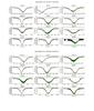 |
Fig. E.10 Observed spectra, the 95% probability models (green) and the best fit model (red) for VFTS 153 and 160. The vertical dashed lines indicate the wavelength range used to fit the corresponding diagnostic line. |
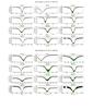 |
Fig. E.11 Observed spectra, the 95% probability models (green) and the best fit model (red) for VFTS 171 and 172. The vertical dashed lines indicate the wavelength range used to fit the corresponding diagnostic line. |
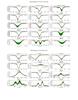 |
Fig. E.12 Observed spectra, the 95% probability models (green) and the best fit model (red) for VFTS 178 and 180. The vertical dashed lines indicate the wavelength range used to fit the corresponding diagnostic line. |
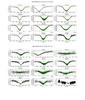 |
Fig. E.13 Observed spectra, the 95% probability models (green) and the best fit model (red) for VFTS 185 and 188. The vertical dashed lines indicate the wavelength range used to fit the corresponding diagnostic line. |
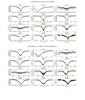 |
Fig. E.14 Observed spectra, the 95% probability models (green) and the best fit model (red) for VFTS 192 and 205. The vertical dashed lines indicate the wavelength range used to fit the corresponding diagnostic line. |
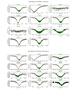 |
Fig. E.15 Observed spectra, the 95% probability models (green) and the best fit model (red) for VFTS 207 and 210. The vertical dashed lines indicate the wavelength range used to fit the corresponding diagnostic line. |
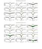 |
Fig. E.16 Observed spectra, the 95% probability models (green) and the best fit model (red) for VFTS 226 and 235. The vertical dashed lines indicate the wavelength range used to fit the corresponding diagnostic line. |
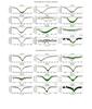 |
Fig. E.17 Observed spectra, the 95% probability models (green) and the best fit model (red) for VFTS 244 and 253. The vertical dashed lines indicate the wavelength range used to fit the corresponding diagnostic line. |
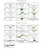 |
Fig. E.18 Observed spectra, the 95% probability models (green) and the best fit model (red) for VFTS 259 and 267. The vertical dashed lines indicate the wavelength range used to fit the corresponding diagnostic line. |
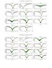 |
Fig. E.19 Observed spectra, the 95% probability models (green) and the best fit model (red) for VFTS 304 and 306. The vertical dashed lines indicate the wavelength range used to fit the corresponding diagnostic line. |
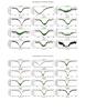 |
Fig. E.20 Observed spectra, the 95% probability models (green) and the best fit model (red) for VFTS 328 and 332. The vertical dashed lines indicate the wavelength range used to fit the corresponding diagnostic line. |
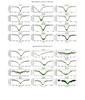 |
Fig. E.21 Observed spectra, the 95% probability models (green) and the best fit model (red) for VFTS 333 and 346. The vertical dashed lines indicate the wavelength range used to fit the corresponding diagnostic line. |
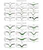 |
Fig. E.22 Observed spectra, the 95% probability models (green) and the best fit model (red) for VFTS 370 and 399. The vertical dashed lines indicate the wavelength range used to fit the corresponding diagnostic line. |
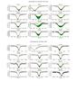 |
Fig. E.23 Observed spectra, the 95% probability models (green) and the best fit model (red) for VFTS 440 and 466. The vertical dashed lines indicate the wavelength range used to fit the corresponding diagnostic line. |
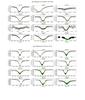 |
Fig. E.24 Observed spectra, the 95% probability models (green) and the best fit model (red) for VFTS 495 and 502. The vertical dashed lines indicate the wavelength range used to fit the corresponding diagnostic line. |
 |
Fig. E.25 Observed spectra, the 95% probability models (green) and the best fit model (red) for VFTS 503 and 513. The vertical dashed lines indicate the wavelength range used to fit the corresponding diagnostic line. |
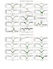 |
Fig. E.26 Observed spectra, the 95% probability models (green) and the best fit model (red) for VFTS 518 and 546. The vertical dashed lines indicate the wavelength range used to fit the corresponding diagnostic line. |
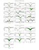 |
Fig. E.27 Observed spectra, the 95% probability models (green) and the best fit model (red) for VFTS 566 and 569. The vertical dashed lines indicate the wavelength range used to fit the corresponding diagnostic line. |
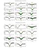 |
Fig. E.28 Observed spectra, the 95% probability models (green) and the best fit model (red) for VFTS 571 and 574. The vertical dashed lines indicate the wavelength range used to fit the corresponding diagnostic line. |
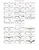 |
Fig. E.29 Observed spectra, the 95% probability models (green) and the best fit model (red) for VFTS 599 and 607. The vertical dashed lines indicate the wavelength range used to fit the corresponding diagnostic line. |
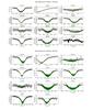 |
Fig. E.30 Observed spectra, the 95% probability models (green) and the best fit model (red) for VFTS 615 and 620. |
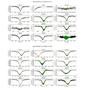 |
Fig. E.31 Observed spectra, the 95% probability models (green) and the best fit model (red) for VFTS 622 and 664. The vertical dashed lines indicate the wavelength range used to fit the corresponding diagnostic line. |
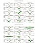 |
Fig. E.32 Observed spectra, the 95% probability models (green) and the best fit model (red) for VFTS 669 and 711. The vertical dashed lines indicate the wavelength range used to fit the corresponding diagnostic line. |
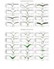 |
Fig. E.33 Observed spectra, the 95% probability models (green) and the best fit model (red) for VFTS 753 and 764. The vertical dashed lines indicate the wavelength range used to fit the corresponding diagnostic line. |
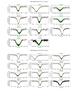 |
Fig. E.34 Observed spectra, the 95% probability models (green) and the best fit model (red) for VFTS 777 and 782. The vertical dashed lines indicate the wavelength range used to fit the corresponding diagnostic line. |
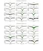 |
Fig. E.35 Observed spectra, the 95% probability models (green) and the best fit model (red) for VFTS 787 and 807. |
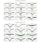 |
Fig. E.36 Observed spectra, the 95% probability models (green) and the best fit model (red) for VFTS 819 and 843. The vertical dashed lines indicate the wavelength range used to fit the corresponding diagnostic line. |
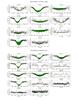 |
Fig. E.37 Observed spectra, the 95% probability models (green) and the best fit model (red) for VFTS 051 and 125. |
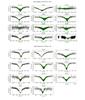 |
Fig. E.38 Observed spectra, the 95% probability models (green) and the best fit model (red) for VFTS 131 and 142. The vertical dashed lines indicate the wavelength range used to fit the corresponding diagnostic line. |
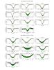 |
Fig. E.39 Observed spectra, the 95% probability models (green) and the best fit model (red) for VFTS 145 and 177. The vertical dashed lines indicate the wavelength range used to fit the corresponding diagnostic line. |
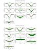 |
Fig. E.40 Observed spectra, the 95% probability models (green) and the best fit model (red) for VFTS 208 and 360. The vertical dashed lines indicate the wavelength range used to fit the corresponding diagnostic line. |
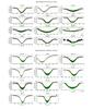 |
Fig. E.41 Observed spectra, the 95% probability models (green) and the best fit model (red) for VFTS 373 and 393. The vertical dashed lines indicate the wavelength range used to fit the corresponding diagnostic line. |
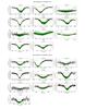 |
Fig. E.42 Observed spectra, the 95% probability models (green) and the best fit model (red) for VFTS 400 and 405. The vertical dashed lines indicate the wavelength range used to fit the corresponding diagnostic line. |
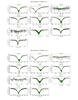 |
Fig. E.43 Observed spectra, the 95% probability models (green) and the best fit model (red) for VFTS 412 and 444. The vertical dashed lines indicate the wavelength range used to fit the corresponding diagnostic line. |
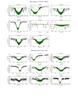 |
Fig. E.44 Observed spectra, the 95% probability models (green) and the best fit model (red) for VFTS 446 and 451. The vertical dashed lines indicate the wavelength range used to fit the corresponding diagnostic line. |
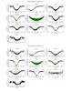 |
Fig. E.45 Observed spectra, the 95% probability models (green) and the best fit model (red) for VFTS 456 and 465. The vertical dashed lines indicate the wavelength range used to fit the corresponding diagnostic line. |
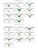 |
Fig. E.46 Observed spectra, the 95% probability models (green) and the best fit model (red) for VFTS 476 and 477. The vertical dashed lines indicate the wavelength range used to fit the corresponding diagnostic line. |
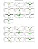 |
Fig. E.47 Observed spectra, the 95% probability models (green) and the best fit model (red) for VFTS 515 and 519. The vertical dashed lines indicate the wavelength range used to fit the corresponding diagnostic line. |
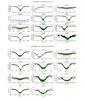 |
Fig. E.48 Observed spectra, the 95% probability models (green) and the best fit model (red) for VFTS 528 and 529. The vertical dashed lines indicate the wavelength range used to fit the corresponding diagnostic line. |
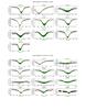 |
Fig. E.49 Observed spectra, the 95% probability models (green) and the best fit model (red) for VFTS 539 and 559. The vertical dashed lines indicate the wavelength range used to fit the corresponding diagnostic line. |
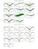 |
Fig. E.50 Observed spectra, the 95% probability models (green) and the best fit model (red) for VFTS 565 and 579. The vertical dashed lines indicate the wavelength range used to fit the corresponding diagnostic line. |
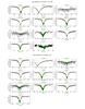 |
Fig. E.51 Observed spectra, the 95% probability models (green) and the best fit model (red) for VFTS 587 and 594. The vertical dashed lines indicate the wavelength range used to fit the corresponding diagnostic line. |
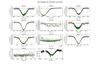 |
Fig. E.52 Observed spectra, the 95% probability models (green) and the best fit model (red) for VFTS 626. The vertical dashed lines indicate the wavelength range used to fit the corresponding diagnostic line. |
All Tables
Teff −SpT linear-fit parameters and their 1σ error bars derived for stars with spectral subtypes O3 to O9 in the combined sample (see text).
Frequency of stars from different sub-samples that display a helium abundance by mass (Y) larger than the specified limit by at least 2σY.
Coefficients describing empirical and theoretical modified-wind momentum relations.
List of the diagnostic lines for the O giants, bright giants, and supergiants for which hydrogen, helium, and nitrogen have been included and used simultaneously in the determination of the stellar and wind parameters.
List of the H and He diagnostic lines included in the analysis of the O giants, bright giants, and supergiants.
List of the H and He diagnostic lines included in the analysis of O stars without luminosity class.
Best-fitting atmospheric and wind parameters of the stars with no luminosity class.
All Figures
|
Fig. 1 Spectral-type distribution of the O-type stars in our sample, binned per spectral subtype (SpT). Different colors and shadings indicate different luminosity classes (LC); see legend. The legend also gives the total number of stars in each LC class (e.g., 40 LC III). In parentheses we provide the number of stars that were given an ambiguous LC classification within each category in Walborn et al. (2014) (e.g., 3 in LC III). They are plotted in their corresponding category with lower opacity (see main text for details). |
| In the text | |
|
Fig. 2 Spatial distribution of the presumably single O-type stars as a function of LC. North is to the top; east is to the left. The circles define regions within 2.4′ of NGC 2070 (central circle) and NGC 2060 (south-west circle). Different symbols indicate LC: III (circles), II (squares), I (triangles). Note that because of crowding a considerable fraction of the sources overlap. Lower opacities again denote sources with an ambiguous LC classification, similar as in Fig. 1. |
| In the text | |
|
Fig. 3 Range of each fitted parameter (left panels of each set) and accompanying range of 95% confidence interval (right panel of each set) in the same unit. Colors have been used to differentiate between stars that have been analyzed using hydrogen and helium lines (HHe) and those for which also nitrogen lines (HHeN) were considered (see also Sect. 3.1). The distributions exclude stars for which only upper/lower limits could be determined, hence the number of stars shown in a panel depends on the parameter that is investigated. In each panel, the median value and the 16th and 84th percentiles are shown using vertical lines. |
| In the text | |
|
Fig. 4 Effective temperature vs. spectral subtype for the O-type with well defined LC (see main text). The lower-opacity symbols give the results for the sample of LMC stars investigated by Mokiem et al. (2007b). |
| In the text | |
|
Fig. 5 Effective temperature vs. spectral subtype but now displaying fits that combine our sample with that of Mokiem et al. (2007b): CS = Combined sample (see main text). Stars with spectral subtype O2-3 or later than O9 have been plotted with lower opacity. The dashed lines give the theoretical calibrations of Martins et al. (2005) for Galactic class III and I stars. The leading number in the legend refers to the total number of O3-O9 stars for which the fit has been derived. The trailing number refers to the total number of stars in each sample. |
| In the text | |
|
Fig. 6 log gc vs. log Teff (upper panel) and spectroscopic Hertzsprung-Russell (lower panel) diagrams of the O-type giants, bright giants, and supergiants, where |
| In the text | |
|
Fig. 7 Helium mass fraction Y versus νesini (upper panel) and log gc (lower panel). Symbols and colors have the same meaning as in Fig. 5. Gray diamonds denote stars with LC III to I from Mokiem et al. (2007a). The purple dashed line at Y = 0.255 defines the initial composition for LMC stars; the gray bar is the 3σ uncertainty in this number. |
| In the text | |
|
Fig. 8 Helium mass fraction Y versus the empirical (unclumped) mass-loss rate relative to the stellar mass (Ṁ/M) for our sample stars with their respective 95% confidence intervals. Added to this is the set of very massive luminous O, Of, Of/WN and WNh stars analyzed in Paper XVII, excluding the nine stars in common with this paper. Also shown are evolutionary tracks by Brott et al. (2011) and Köhler et al. (2015) for stars with initial spin rates of approximately 200 kms-1 (upper panel) and 300 kms-1 (lower panel) with dots every 1 Myr of evolution. These tracks are truncated at 30 kK, which is approximately the temperature where the stars evolve into B-type objects and thus are no longer part of our observational sample. |
| In the text | |
|
Fig. 9 Two versions of the Hertzsprung-Russell diagram. In the top panel our sample of single O-type giants and supergiants is supplemented with the dwarf O star sample of Paper XIII and the sample of very massive Of and WNh stars by Paper XVII. We exclude the results of Paper XVII for the nine stars in common with this paper and adopted our results (see Sect. 3.4.3). Symbols and colors have the same meaning as in Fig. 6. The lower panel only contains the sample studied here. The symbol shapes in the lower panel show three categories of helium mass fraction, that is, not enriched (squares), moderately enriched (triangles), and enriched (stars). The symbol colors refer to their projected rotational velocity (see color bar on the right). Evolutionary tracks and isochrones are for models that have an initial rotational velocity of approximately 200 kms-1 (Brott et al. 2011; Köhler et al. 2015). Iso-helium lines for different rotational velocities are from Köhler et al. (2015) and are color-coded using the color bar. |
| In the text | |
|
Fig. 10 Modified wind momentum (Dmom) vs. luminosity diagram. The dashed lines indicate the theoretical predictions of Vink et al. (2001) for homogeneous winds. Top panel: the empirical fit for this work and Mokiem et al. (2007a) (both for L/L⊙> 5.0) in shaded blue and gray bars, respectively. For stars with L/L⊙ ≤ 5.0, only upper limits could be constrained. These stars are not considered in the analysis. Bottom panel: same as top panel but now for an analysis in which the acceleration of the wind flow, β, is a free parameter and in which the analysis does not include nitrogen lines, but relies on hydrogen and helium lines only. |
| In the text | |
|
Fig. 11 Comparison of spectroscopic masses and evolutionary masses for the 66 sources that have Mevol constrained by bonnsai. The upper panel shows a one-to-one comparison; the lower panel shows the ratio of the masses. |
| In the text | |
|
Fig. 12 Mass discrepancy plotted against luminosity for the 66 sources that have Mevol constrained by bonnsai. The upper dashed line is from the L(M) relation of helium stars; see main text for discussion. The lower line is Mspec = Mevol, and is a lower limit as stars cannot be under-luminous. The color denotes the surface helium abundance. Squares denote stars for which the LC is certain and triangles refer to the sources with weak Si iv relative to He i and for which the luminosity class may be debated (they may be dwarf stars). Helium enriched sources are all positioned above the one-to-one relation. |
| In the text | |
|
Fig. A.1 Cumulative (upper panel) and frequency (middle panel) distributions of the projected rotational velocities of the O-type LC III to I as derived here from the automated fastwind analysis and Paper XII. The middle panel shows Poissonian error bars. The lower panel compares the actual νesini of these two samples. |
| In the text | |
|
Fig. B.1 Hertzsprung-Russell diagram of the sample as a function of spatial location: NGC 2070 (upper panel), NGC 2060 (middle panel) and stars outside star-forming complexes (lower panel). Evolutionary tracks (solid lines) and isochrones (dot-dashed lines) are from stellar models initially rotating with approximately 200 kms-1 (Brott et al. 2011; Köhler et al. 2015). |
| In the text | |
|
Fig. E.1 Observed spectra, the 95% probability models (green) and the best fit model (red) for VFTS 016 and 035. The vertical dashed lines indicate the wavelength range used to fit the corresponding diagnostic line. |
| In the text | |
|
Fig. E.2 Observed spectra, the 95% probability models (green) and the best fit model (red) for VFTS 046 and 064. The vertical dashed lines indicate the wavelength range used to fit the corresponding diagnostic line. |
| In the text | |
|
Fig. E.3 Observed spectra, the 95% probability models (green) and the best fit model (red) for VFTS 070 and 076. The vertical dashed lines indicate the wavelength range used to fit the corresponding diagnostic line. |
| In the text | |
|
Fig. E.4 Observed spectra, the 95% probability models (green) and the best fit model (red) for VFTS 077 and 080. The vertical dashed lines indicate the wavelength range used to fit the corresponding diagnostic line. |
| In the text | |
|
Fig. E.5 Observed spectra, the 95% probability models (green) and the best fit model (red) for VFTS 087 and 091. The vertical dashed lines indicate the wavelength range used to fit the corresponding diagnostic line. |
| In the text | |
|
Fig. E.6 Observed spectra, the 95% probability models (green) and the best fit model (red) for VFTS 093 and 103. The vertical dashed lines indicate the wavelength range used to fit the corresponding diagnostic line. |
| In the text | |
|
Fig. E.7 Observed spectra, the 95% probability models (green) and the best fit model (red) for VFTS 104 and 109. The vertical dashed lines indicate the wavelength range used to fit the corresponding diagnostic line. |
| In the text | |
|
Fig. E.8 Observed spectra, the 95% probability models (green) and the best fit model (red) for VFTS 113 and 128. The vertical dashed lines indicate the wavelength range used to fit the corresponding diagnostic line. |
| In the text | |
|
Fig. E.9 Observed spectra, the 95% probability models (green) and the best fit model (red) for VFTS 141 and 151. The vertical dashed lines indicate the wavelength range used to fit the corresponding diagnostic line. |
| In the text | |
|
Fig. E.10 Observed spectra, the 95% probability models (green) and the best fit model (red) for VFTS 153 and 160. The vertical dashed lines indicate the wavelength range used to fit the corresponding diagnostic line. |
| In the text | |
|
Fig. E.11 Observed spectra, the 95% probability models (green) and the best fit model (red) for VFTS 171 and 172. The vertical dashed lines indicate the wavelength range used to fit the corresponding diagnostic line. |
| In the text | |
|
Fig. E.12 Observed spectra, the 95% probability models (green) and the best fit model (red) for VFTS 178 and 180. The vertical dashed lines indicate the wavelength range used to fit the corresponding diagnostic line. |
| In the text | |
|
Fig. E.13 Observed spectra, the 95% probability models (green) and the best fit model (red) for VFTS 185 and 188. The vertical dashed lines indicate the wavelength range used to fit the corresponding diagnostic line. |
| In the text | |
|
Fig. E.14 Observed spectra, the 95% probability models (green) and the best fit model (red) for VFTS 192 and 205. The vertical dashed lines indicate the wavelength range used to fit the corresponding diagnostic line. |
| In the text | |
|
Fig. E.15 Observed spectra, the 95% probability models (green) and the best fit model (red) for VFTS 207 and 210. The vertical dashed lines indicate the wavelength range used to fit the corresponding diagnostic line. |
| In the text | |
|
Fig. E.16 Observed spectra, the 95% probability models (green) and the best fit model (red) for VFTS 226 and 235. The vertical dashed lines indicate the wavelength range used to fit the corresponding diagnostic line. |
| In the text | |
|
Fig. E.17 Observed spectra, the 95% probability models (green) and the best fit model (red) for VFTS 244 and 253. The vertical dashed lines indicate the wavelength range used to fit the corresponding diagnostic line. |
| In the text | |
|
Fig. E.18 Observed spectra, the 95% probability models (green) and the best fit model (red) for VFTS 259 and 267. The vertical dashed lines indicate the wavelength range used to fit the corresponding diagnostic line. |
| In the text | |
|
Fig. E.19 Observed spectra, the 95% probability models (green) and the best fit model (red) for VFTS 304 and 306. The vertical dashed lines indicate the wavelength range used to fit the corresponding diagnostic line. |
| In the text | |
|
Fig. E.20 Observed spectra, the 95% probability models (green) and the best fit model (red) for VFTS 328 and 332. The vertical dashed lines indicate the wavelength range used to fit the corresponding diagnostic line. |
| In the text | |
|
Fig. E.21 Observed spectra, the 95% probability models (green) and the best fit model (red) for VFTS 333 and 346. The vertical dashed lines indicate the wavelength range used to fit the corresponding diagnostic line. |
| In the text | |
|
Fig. E.22 Observed spectra, the 95% probability models (green) and the best fit model (red) for VFTS 370 and 399. The vertical dashed lines indicate the wavelength range used to fit the corresponding diagnostic line. |
| In the text | |
|
Fig. E.23 Observed spectra, the 95% probability models (green) and the best fit model (red) for VFTS 440 and 466. The vertical dashed lines indicate the wavelength range used to fit the corresponding diagnostic line. |
| In the text | |
|
Fig. E.24 Observed spectra, the 95% probability models (green) and the best fit model (red) for VFTS 495 and 502. The vertical dashed lines indicate the wavelength range used to fit the corresponding diagnostic line. |
| In the text | |
|
Fig. E.25 Observed spectra, the 95% probability models (green) and the best fit model (red) for VFTS 503 and 513. The vertical dashed lines indicate the wavelength range used to fit the corresponding diagnostic line. |
| In the text | |
|
Fig. E.26 Observed spectra, the 95% probability models (green) and the best fit model (red) for VFTS 518 and 546. The vertical dashed lines indicate the wavelength range used to fit the corresponding diagnostic line. |
| In the text | |
|
Fig. E.27 Observed spectra, the 95% probability models (green) and the best fit model (red) for VFTS 566 and 569. The vertical dashed lines indicate the wavelength range used to fit the corresponding diagnostic line. |
| In the text | |
|
Fig. E.28 Observed spectra, the 95% probability models (green) and the best fit model (red) for VFTS 571 and 574. The vertical dashed lines indicate the wavelength range used to fit the corresponding diagnostic line. |
| In the text | |
|
Fig. E.29 Observed spectra, the 95% probability models (green) and the best fit model (red) for VFTS 599 and 607. The vertical dashed lines indicate the wavelength range used to fit the corresponding diagnostic line. |
| In the text | |
|
Fig. E.30 Observed spectra, the 95% probability models (green) and the best fit model (red) for VFTS 615 and 620. |
| In the text | |
|
Fig. E.31 Observed spectra, the 95% probability models (green) and the best fit model (red) for VFTS 622 and 664. The vertical dashed lines indicate the wavelength range used to fit the corresponding diagnostic line. |
| In the text | |
|
Fig. E.32 Observed spectra, the 95% probability models (green) and the best fit model (red) for VFTS 669 and 711. The vertical dashed lines indicate the wavelength range used to fit the corresponding diagnostic line. |
| In the text | |
|
Fig. E.33 Observed spectra, the 95% probability models (green) and the best fit model (red) for VFTS 753 and 764. The vertical dashed lines indicate the wavelength range used to fit the corresponding diagnostic line. |
| In the text | |
|
Fig. E.34 Observed spectra, the 95% probability models (green) and the best fit model (red) for VFTS 777 and 782. The vertical dashed lines indicate the wavelength range used to fit the corresponding diagnostic line. |
| In the text | |
|
Fig. E.35 Observed spectra, the 95% probability models (green) and the best fit model (red) for VFTS 787 and 807. |
| In the text | |
|
Fig. E.36 Observed spectra, the 95% probability models (green) and the best fit model (red) for VFTS 819 and 843. The vertical dashed lines indicate the wavelength range used to fit the corresponding diagnostic line. |
| In the text | |
|
Fig. E.37 Observed spectra, the 95% probability models (green) and the best fit model (red) for VFTS 051 and 125. |
| In the text | |
|
Fig. E.38 Observed spectra, the 95% probability models (green) and the best fit model (red) for VFTS 131 and 142. The vertical dashed lines indicate the wavelength range used to fit the corresponding diagnostic line. |
| In the text | |
|
Fig. E.39 Observed spectra, the 95% probability models (green) and the best fit model (red) for VFTS 145 and 177. The vertical dashed lines indicate the wavelength range used to fit the corresponding diagnostic line. |
| In the text | |
|
Fig. E.40 Observed spectra, the 95% probability models (green) and the best fit model (red) for VFTS 208 and 360. The vertical dashed lines indicate the wavelength range used to fit the corresponding diagnostic line. |
| In the text | |
|
Fig. E.41 Observed spectra, the 95% probability models (green) and the best fit model (red) for VFTS 373 and 393. The vertical dashed lines indicate the wavelength range used to fit the corresponding diagnostic line. |
| In the text | |
|
Fig. E.42 Observed spectra, the 95% probability models (green) and the best fit model (red) for VFTS 400 and 405. The vertical dashed lines indicate the wavelength range used to fit the corresponding diagnostic line. |
| In the text | |
|
Fig. E.43 Observed spectra, the 95% probability models (green) and the best fit model (red) for VFTS 412 and 444. The vertical dashed lines indicate the wavelength range used to fit the corresponding diagnostic line. |
| In the text | |
|
Fig. E.44 Observed spectra, the 95% probability models (green) and the best fit model (red) for VFTS 446 and 451. The vertical dashed lines indicate the wavelength range used to fit the corresponding diagnostic line. |
| In the text | |
|
Fig. E.45 Observed spectra, the 95% probability models (green) and the best fit model (red) for VFTS 456 and 465. The vertical dashed lines indicate the wavelength range used to fit the corresponding diagnostic line. |
| In the text | |
|
Fig. E.46 Observed spectra, the 95% probability models (green) and the best fit model (red) for VFTS 476 and 477. The vertical dashed lines indicate the wavelength range used to fit the corresponding diagnostic line. |
| In the text | |
|
Fig. E.47 Observed spectra, the 95% probability models (green) and the best fit model (red) for VFTS 515 and 519. The vertical dashed lines indicate the wavelength range used to fit the corresponding diagnostic line. |
| In the text | |
|
Fig. E.48 Observed spectra, the 95% probability models (green) and the best fit model (red) for VFTS 528 and 529. The vertical dashed lines indicate the wavelength range used to fit the corresponding diagnostic line. |
| In the text | |
|
Fig. E.49 Observed spectra, the 95% probability models (green) and the best fit model (red) for VFTS 539 and 559. The vertical dashed lines indicate the wavelength range used to fit the corresponding diagnostic line. |
| In the text | |
|
Fig. E.50 Observed spectra, the 95% probability models (green) and the best fit model (red) for VFTS 565 and 579. The vertical dashed lines indicate the wavelength range used to fit the corresponding diagnostic line. |
| In the text | |
|
Fig. E.51 Observed spectra, the 95% probability models (green) and the best fit model (red) for VFTS 587 and 594. The vertical dashed lines indicate the wavelength range used to fit the corresponding diagnostic line. |
| In the text | |
|
Fig. E.52 Observed spectra, the 95% probability models (green) and the best fit model (red) for VFTS 626. The vertical dashed lines indicate the wavelength range used to fit the corresponding diagnostic line. |
| In the text | |
Current usage metrics show cumulative count of Article Views (full-text article views including HTML views, PDF and ePub downloads, according to the available data) and Abstracts Views on Vision4Press platform.
Data correspond to usage on the plateform after 2015. The current usage metrics is available 48-96 hours after online publication and is updated daily on week days.
Initial download of the metrics may take a while.