| Issue |
A&A
Volume 599, March 2017
|
|
|---|---|---|
| Article Number | A43 | |
| Number of page(s) | 23 | |
| Section | Extragalactic astronomy | |
| DOI | https://doi.org/10.1051/0004-6361/201628849 | |
| Published online | 24 February 2017 | |
Colors of barlenses: evidence for connecting them to boxy/peanut bulges
1 Astronomy Research Unit, University of Oulu, 90014 Oulu, Finland
e-mail: This email address is being protected from spambots. You need JavaScript enabled to view it.
2 Instituto de Astrofísica de Canarias, 38200 La Laguna, Tenerife, Spain
3 Departamento de Astrofísica, Universidad de La Laguna, 38205 La Laguna, Tenerife, Spain
Received: 3 May 2016
Accepted: 7 September 2016
Abstract
Aims. We aim to study the colors and orientations of structures in low and intermediate inclination barred galaxies. We test the hypothesis that barlenses, roundish central components embedded in bars, could form part of the bar in a similar manner to boxy/peanut bulges in the edge-on view.
Methods. A sample of 79 barlens galaxies was selected from the Spitzer Survey of Stellar Structure in Galaxies (S4G) and the Near IR S0 galaxy Survey (NIRS0S), based on previous morphological classifications at 3.6 μm and 2.2 μm wavelengths. For these galaxies the sizes, ellipticities, and orientations of barlenses were measured, parameters which were used to define the barlens regions in the color measurements. In particular, the orientations of barlenses were studied with respect to those of the “thin bars” and the line-of-nodes of the disks. For a subsample of 47 galaxies color index maps were constructed using the Sloan Digital Sky Survey (SDSS) images in five optical bands, u, g, r, i, and z. Colors of bars, barlenses, disks, and central regions of the galaxies were measured using two different approaches and color−color diagrams sensitive to metallicity, stellar surface gravity, and short lived stars were constructed. Color differences between the structure components were also calculated for each individual galaxy, and presented in histogram form.
Results. We find that the colors of barlenses are very similar to those of the surrounding bars, indicating that most probably they form part of the bar. We also find that barlenses have orientations closer to the disk line-of-nodes than to the thin bars, which is consistent with the idea that they are vertically thick, in a similar manner as the boxy/peanut structures in more inclined galaxies. Typically, the colors of barlenses are also similar to those of normal E/S0 galaxies. Galaxy by galaxy studies also show that in spiral galaxies very dusty barlenses also exist, along with barlenses with rejuvenated stellar populations. The central regions of galaxies are found to be on average redder than bars or barlenses, although galaxies with bluer central peaks also exist.
Key words: galaxies: structure / galaxies: bulges
© ESO, 2017
1. Introduction
Galactic bulges is an active research topic, not least because of the recent discoveries concerning the Milky Way bulge, which is now known to form part of the Milky Way bar (Weiland et al. 1994). Photometrically bulges are defined as flux above the underlying disk, and observers often divide them into “classical bulges”, which are highly relaxed, velocity dispersion supported spheroidal components, and rotationally supported pseudo-bulges, which originate from the disk material (Kormendy 1983). The formation of a pseudo-bulge is associated to the evolution of a bar, which can vertically thicken the central bar regions, for example by bar buckling effects (Combes et al. 1990; Raha et al. 1991; Pfenniger & Friedli 1991), leading to boxy- or peanut-shaped bulges (see Athanassoula 2005). Bars can also trigger gas inflows, which, via star formation, can collect stars to the central regions of the galaxies, manifested as central disks (i.e., “disky pseudo-bulges”). Classical and pseudo-bulges are often distinguished via low Sérsic indices (n ~ 1 means a pseudo-bulge) and low bulge-to-total flux ratios, but this approach has shown out to be oversimplified (see review by Kormendy 2016). More sophisticated multi-parameter methods, including kinematics, stellar populations, and metallicities, have been developed, of which an update is given by Fisher & Drory (2016). However, all these methods have been developed for separating classical bulges from inner disks (i.e., disky pseudo-bulges), without paying attention to the vertically thick inner bar components, which might be visible at a large range of galaxy inclinations.
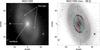 |
Fig. 1 Example barlens galaxy, NGC 1350. Left panel: the bar region of the 3.6 μm image. Marked are the structure components measured in this study: “bl” refers to barlens, “thin bar” is the bar region outside the barlens, and “nucleus” refers to possible small bulge in the central regions. Right panel: the contours of the same image. Lines indicating the orientations of the bar (blue line), barlens (red line), and the disk line-of-nodes (dashed line) are over-plotted. Black crosses show the points selected to measure the size and orientation of the barlens by fitting an ellipse to these points. |
In fact, there has been a long-standing ambiguity in interpreting bulges at low and high galaxy inclinations in the nearby Universe. While in the edge-on view many bulges have boxy or peanut shape isophotes and are thereby associated with bars (Lütticke et al. 2000; Bureau et al. 2006), in less inclined galaxies the central flux concentrations in a large majority of galaxies have been interpreted in terms of classical bulges (see the discussion by Laurikainen & Salo 2016). Isophotal analysis (Athanassoula & Beaton 2006; Erwin & Debattista 2013) have shown that boxy/peanut bulges, based on their isophotal orientation with respect to the bar and the galaxy line-of-nodes, can be identified even at fairly low galaxy inclinations. In a few galaxies boxy/peanut bulges have been identified also kinematically (Méndez-Abreu et al. 2008, 2014) in almost face-on view, but such observations are difficult to make.
As a solution to the puzzle of how boxy/peanut bulges appear in nearly face-on galaxies, Laurikainen et al. (2014) suggested that they manifest as barlenses, that is, central lens-like morphologies embedded in bars. Based on multi-component structural decompositions they showed that among the Milky Way mass galaxies such vertically thick bar components might contain most of the bulge mass in the local Universe. Theoretical evidence for the idea that barlenses and boxy/peanut bulges might be one and the same component was given by Athanassoula et al. (2015), where detailed comparisons of simulation models with such properties as size and ellipticity of a barlens were made. If the above interpretation is correct, we would expect barlenses at intermediate galaxy inclinations to appear in isophotal analysis in a similar manner as the boxy/peanut structures. Moreover, the colors of barlenses can be compared with those of the bars outside the barlens regions in order to look for similarities. However, the colors of barlenses have not been studied yet, and also, there are no theoretical models in which the colors were directly predicted. Our hypothesis in this study is that if barlenses (in a similar manner as boxy/peanut bulges) are formed of the same material as the rest of the bar, their colors should be similar to those of the rest of the bar.
Barlenses were recognized and coded into morphological classification by Laurikainen et al. (2011) for the Near IR S0 galaxy Survey (NIRS0S), and by Buta et al. (2015) at 3.6 μm for the Spitzer Survey of Stellar Structure in Galaxies (S4G; Sheth et al. 2010). Nuclear bars, rings and lenses are embedded in barlenses in many galaxies, but their sizes are always smaller than those of barlenses. An example of a barlens galaxy, NGC 1350, is shown in Fig. 1 (left panel), where the different structure components in the bar region are illustrated. The bar region outside the barlens is called the “thin bar” (or simply bar), considering that it is assumed to be vertically thin. Depending on the level of gas accretion and the subsequent star formation histories of barlens galaxies, the central components can have variable colors. However, any classical bulges that might appear in these galaxies are expected to be dominated by old stellar populations. The spheroidals are dynamically hot and therefore any accretion of external gas into these components would be difficult.
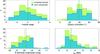 |
Fig. 2 Distributions of morphological type, inclination, absolute B magnitude, and bar size, for the whole sample of barlens galaxies (green histogram), and for the subsample of galaxies with SDSS imaging (blue histogram). The green solid and blue dashed vertical lines show the median values of the distributions for the complete and color subsample, respectively. |
2. Sample and data
2.1. Sample
Our sample consists of a set of barlens galaxies from two near-infrared galaxy surveys. The Spitzer Survey of Stellar Structure in Galaxies (Sheth et al. 2010, hereafter S4G) which contains 2352 galaxies observed at 3.6 and 4.5 μm with the Infrared Array Camera (IRAC; Fazio et al. 2004) on board the Spitzer Space Telescope. This survey is limited in volume (distance d< 40 Mpc, Galactic latitude | b | > 30 deg), magnitude (Bcorr< 15.5 mag, corrected for internal extinction) and size (D25> 1 arcmin). It covers all Hubble types and disk inclinations. From this survey we selected all galaxies with barlenses in the classification by Buta et al. (2015). In that study no inclination limit was used, however the barlens galaxies have in general inclination ≲60°. Only in one case the inclination is ~71°. The other survey is the NIRS0S (Laurikainen et al. 2011), which consists of ~200 early-type disk galaxies observed in the Ks-band, with total magnitude BT ≤ 12.5 mag. The inclination limit of this sample is 65°. Altogether, S4G and NIRS0S contain 79 barlens galaxies. If not otherwise mentioned that forms our sample in all the following. This sample will be used to study the orientation of barlenses with respect to those of the bar and the disk line-of-nodes. Of these galaxies 22 appear both in NIRS0S and S4G, and NIRS0S has 11 barlens galaxies which do not form part of S4G. The barlens galaxy sample is the same as used by Laurikainen et al. (2014).
2.2. Infrared data
The 3.6 μm images from S4G typically reach the surface brightnesses of 26.5 (AB) mag arcsec-2, which translates to roughly 28 mag arcsec-2 in the B-band. These images have a pixel resolution of 0.′′75 and full-width half-maximum (FWHM) ≈ 2′′. The NIRS0S images at 2.2 μm typically reach B-band surface brightnesses of 27 mag arcsec-2, with pixel resolution in the range 0.′′23−0.′′61 (typically 0.′′25). When 3.6 μm images exist they have a priority in our analysis. The complete list of barlens galaxies appear in Table 1 (see Appendix C): shown are the morphological types, orientations (PAdisk) and inclinations (idisk) of the disks. For S4G galaxies the morphological types are from Buta et al. (2015), the orientations and inclinations of the disks are from Salo et al. (2015), and the parameters of bars from Herrera-Endoqui et al. (2015). For NIRS0S galaxies the morphological types and bar and disk parameters are taken from the original paper (Laurikainen et al. 2011). In these references the bar parameters were obtained by both visual and ellipse fitting methods, however, only the visual length (rbar) and orientation (PAbar) are used here. The disk parameters were obtained using isophotal ellipse fits, from which the ellipticity and orientations of the outer isophotes of the disks are derived. The distances are taken from archive data in the respective survey (in the case of S4G galaxies see Muñoz-Mateos et al. 2015). These are redshift independent distances obtained from NED1 when available and otherwise calculated assuming H0 = 71 km s-1 Mpc-1.
2.3. Optical data
In order to obtain the optical colors of the structure components we use the Sloan Digital Sky Survey (York et al. 2000; Gunn et al. 1998, hereafter SDSS) images in five bands: u, g, r, i, and z. The reduced images are taken from Knapen et al. (2014) who used images from SDSS DR7 and SDSS-III DR8 produced from the SDSS photometric pipeline, but using their own sky subtraction. These mosaics are already sky-subtracted and the different bands are aligned with each other. Such mosaiced images exist for all those S4G galaxies for which SDSS data is available, including 47 barlens galaxies. This set of galaxies will be referred to as the “color subsample” in the rest of the paper. The pixel scale in the SDSS images is 0.′′396. These images can be used to derive surface brightness profiles down to μr ~ 27 mag arcsec-2 (Pohlen & Trujillo 2006), equivalent to 27.5 mag arcsec-2 in B-band.
The basic properties, that is, the Hubble stages, galaxy inclinations, optical galaxy magnitudes, and bar sizes, of the complete sample and the color subsample are shown in Fig. 2. The Hubble stage distribution is previously shown also by Laurikainen et al. (2014) for the complete sample. The vertical lines represent the median values of the distributions. For the complete sample these values are Hubble stage T = 0, inclination inc = 38.9°, B absolute magnitude is −19.9 mag, and rbar = 3.1 kpc. In the case of the color subsample the values are T = 0, inc = 38.8°, B absolute magnitude is −19.7 mag, and rbar = 2.9 kpc. We note that the distributions and median properties of the color subsample are very similar to those of the complete sample.
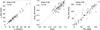 |
Fig. 3 Sizes (rbl), axial ratios ((b/a)bl) and position angles (PAbl) of barlenses obtained in this study are compared with those previosuly obtained by Herrera-Endoqui et al. (2015) or Laurikainen et al. (2011). Dotted lines indicate linear fits between the old and new measurements, whereas the dashed line stands for a unit slope. The labels indicate the slope and correlation coefficient of the linear fit. The galaxies that belong to the color subsample are indicated with an open symbol. |
3. Measuring the sizes and orientations of barlenses
3.1. Sizes
Apparent sizes and shapes of all the barlenses in our sample were measured using the infrared images, fitting ellipses to their outer isophotes. For the galaxies in our sample the sizes have been previously measured by Herrera-Endoqui et al. (2015) or Laurikainen et al. (2011), but using a more visual approach. The difference between the two approaches is that while in the previous measurements the edges of barlenses were visually estimated at a certain magnitude scale, in this study they were defined following the outermost isophotes of barlenses indicated by their surface brightnesses (see Table 1). Points were marked on top of the contour, but avoiding the zone dominated by the bar major axis flux. Then an ellipse was automatically fit to those points, which gives the size (rbl), minor-to-major axis ratio ((b/a)bl), and orientation (PAbl) of the barlens. An example of our measurements is shown in Fig. 1 (right panel), and the derived barlens parameters are compared with those of the previous measurements in Fig. 3. In Table 1 we give the measurements of the barlens parameters and their uncertainties, which were calculated from the set of three measurements (unc = stdev/√N, where N = 3 is the number of measurements). The uncertainties in the orientation parameters of the disks were taken from the respective papers. In the case of bars, the uncertainties were calculated in the same manner described above but with N = 2, using the parameters obtained with the visual and ellipse fitting methods in the respective catalogs. Figure 3 indicates that there are no significant systematic differences between the two measurements. In the position angles and b/a-values the scatter easily appears in measurement of structures having low ellipticities, which is the case also with many barlenses. From hereon we use the isophotal measurements obtained in the current study, which were used also to define the zones in our color index measurements (see Sect. 4.2).
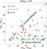 |
Fig. 4 Orientations of barlenses compared with the orientations of bars and those of the lines-of-nodes (disks). The y-axis is the difference between the orientations of the barlens and the disk, whereas the x-axis is the difference between the orientations of the bar and the disk. The differences are given in degrees. Shown are only galaxies where the barlens axial ratio (b/a)bl< 0.9. The galaxies that belong to the color subsample are indicated with an open symbol. |
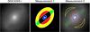 |
Fig. 5 Illustration of the two methods used for defining the regions for the measurements of the component colors. In the left panel the r-band image of NGC 4245 is shown. In the middle panel we show the automatically defined regions for the central region (“nuc1” and “nuc2”; light and dark blue, respectively), for the barlens (“blc”; red), the bar (green), and the disk (yellow), see the text for details. In the right panel the manually selected regions for the barlens, the bar and the disk are shown (central regions are the same as in the middle panel). All images are in the same scale. |
3.2. Orientations
The orientations of barlenses (PAbl) are compared with the orientations of bars (PAbar) and the lines-of-nodes (PAdisk) in Fig. 4. All the orientations were measured in the sky-plane counter-clockwise from the north. The main idea for making this comparison is the following (see also Erwin & Debattista 2013): if barlenses indeed are vertically thick components in a similar manner as boxy/peanut/X-shaped structures of bars (the strongest boxy/peanuts have X-shape morphology), we would expect that to be manifested in their orientations. Namely, it has been demonstrated by simulation models (Bettoni & Galletta 1994; Athanassoula & Beaton 2006) that when the vertically thick boxy/peanut, embedded in a thin bar, is seen in the non-edge-on view, due to an inclination effect the two bar components would have slightly different orientations: the orientation of the boxy/peanut would always be closer to the line-of-nodes than the orientation of the thin bar would be.
In Fig. 4 the galaxies are arbitrarily divided into three galaxy inclination bins (inc < 40°, 40°< inc < 60° and inc > 60°) in order to observe the behavior of the barlens orientation with respect to galaxy inclination. The x-axis shows the orientation difference between the bar and the disk, and the y-axis how much the major-axis barlens orientation deviates from that of the disk. In the diagonal the barlens orientations are along the bar major-axis, and in the horizontal line along the line-of-nodes. Taking into account the measurement uncertainties shown in Fig. 3, it appears that barlenses are oriented between the diagonal and the horizontal line, which is consistent with the idea that they are vertically more extended than the thin bar component. At the lowest galaxy inclinations (inc < 40°) the barlens orientation is more closely along the thin bar, following from their small intrinsic elongation along the thin bar major axis. For higher inclination galaxies (inc > 60°) both the thin bar and the barlens are oriented closer to the line-of-nodes. Contrary to barlenses, none of the boxy/peanut bulges studied by Erwin & Debattista (2013) showed an alignment with the thin bar. This is expected since the galaxies they studied appeared at galaxy inclinations of inc = 45°−65°, where the orientations are expected to fall between the line-of-nodes and the orientation of the thin bar.
4. Obtaining the colors using the SDSS images
4.1. Making the color images
Color maps were constructed in (u−g), (g−r), (r−i), and i−z)-indices for the color subsample. These indices were later used to make color−color diagrams indicative of the different stellar populations and metallicities. The images were rotated so that the bar major axis, determined from the 3.6 or 2.2 μm images, became horizontal. We trust the available sky subtractions, because the original uncertainties that appeared during the SDSS data release were checked by Knapen et al. (2014).
However, before making the color images we needed to be sure that the two images used to make them have the same resolution. For that purpose the Gaussian FWHMs were measured using the IRAF2 task “imexamine”, applied to several field stars in each band for every galaxy. The mean values for the FWHMs are 3.28, 3.07, 2.76, 2.60 and 2.68 pixels in u, g, r, i and z bands, respectively. These values are equivalent to 1.′′30, 1.′′22, 1.′′09, 1.′′03, and 1.′′06, respectively. As discussed by Bergvall et al. (2010) non-Gaussian extended tails at very low surface brightnesses appear, in particular in the i-band. However, although these tails might be important at low surface brightnesses, such effects are not important in our study where only high surface brightness structures are studied. For each color image the higher resolution image was convolved with a Gaussian point spread function (PSF) so that the convolved image had the same FWHM as the lower resolution image. The convolved images were then converted to magnitude-units and corrected for Galactic extinction using the re-calibrated Schlegel et al. (1998) extinctions in the infrared, made by Schlafly & Finkbeiner (2011), assuming a reddening law with RV = 3.1.
4.2. Measuring the colors of the structure components
The convolved images were used to measure the colors of the different structure components. Instead of using directly the color index maps the fluxes in each filter were extracted for the regions defining the structure components. The fluxes in the two bands were then converted to colors applying also the wavelength specific Galactic extinction correction. The colors of the structure components were then measured with two different methods:
Approach 1 (see Fig. 5, middle panel):
Colors of the two bar components, the disks, and the central peaks, were measured using an automatic approach defining the measured regions in the following manner:
nuc1 (central region, light blue color): an elliptical region around the galaxy center was selected having position angle and axis ratio as those of the barlens, and outer radius r = 0.1 × rbl. The region selected this way is smaller than nuclear rings typically are, thus avoiding color contamination from them. Given this definition of nuc1, in 16 galaxies the nuc1 region is smaller than the FWHM of the SDSS image (1.3′′). Our central regions defined by nuc1 go from unresolved to barely resolved nuclei, to much larger regions. In principle this central region could be associated to a small classical bulge, but as the colors alone cannot be used to define bulges, we avoid using that concept.
nuc2 (central region, dark blue color): a similar elliptical region around the galaxy center as above was selected, but using a larger radius, r = 0.3 × rbl. This radius was large enough to cover possible nuclear rings.
bl (barlens): barlens region was taken to be an elliptical zone inside the measured barlens radius. The shape and orientation of this region was defined by the measured b/a and the position angle of the barlens. However, the region covering the central region (nuc2) was excluded.
blc (barlens, red color): this barlens region was otherwise the same as that of bl above, except that the region covering the thin bar (i.e., bar) inside the barlens radius was excluded. The advantage to the previous barlens measurement is that this approach avoids contamination of flux along the bar major axis in the barlens region.
bar (i.e., thin bar, green color): was taken to be an elliptical region inside r = 0.9 × rbar, and outside the barlens. This way we avoid mixing the colors of inner rings with those representing the bars themselves: bars are often surrounded by star forming rings, superimposed with the bars. We used the measured position angle of the bar, and the axial ratio b/a = 0.5 × (b/a)bar. However, as a lower limit to b/a we used b/a = 0.2. For the bar this modified value of b/a was used, because the value that comes out directly from ellipse fitting overestimates the b/a of the thin bar component. This is because the elliptical isophotal shapes are contaminated by the fairly round barlenses sitting inside the bars.
disk (yellow color): for the disk we used an elliptical region inside the radius r = 0.9 × rbar, using the ellipticity and position angle of the barlens. The regions covering the thin bar (green) and everything inside the barlens radius were excluded. The full bar radius was not used because we wanted to avoid possible contamination of inner rings, which often show recent star formation.
Approach 2 (see Fig. 5, right panel):
Specific regions were visually selected and drawn on top of the r-band images. For a barlens two zones at opposite sides of the bar major axis were selected (red color), avoiding the region of the thin bar. The thin bar (green color) was measured in two zones outside the barlens, and avoiding possible star forming inner rings superimposed with the bar. For the disk (yellow color) two zones were selected approximately at the same radial distances where the edges of the thin bar appear.
Color index measurements for the structures of the galaxies in the color subsample.
The measurements using the two approaches are given in Table 1, where the mean and median, and minimum and maximum colors, for each structure component are shown. Also given are the standard error of the mean, obtained by dividing the sample standard deviation with √N. The advantage of approach 1 is that the measurements can be carried out automatically. It also gives a robust manner to include a maximum number of pixels for obtaining the colors of barlenses and thin bars. Approach 2 is more human guided and makes possible to avoid any obviously visible and unwanted star forming regions that might contaminate the color. In spite of these differences the obtained colors in the two measurements are fairly similar. In Table 1 we present data for only 45 of the 47 galaxies in the color subsample. The optical images of NGC 3384 contain artifacts perhaps produced at the mosaicking stage, thus affecting the measurement of the colors. This can be observed as fringes in the resulting color maps (see Appendix A). The case of NGC 4448 is an unfortunate combination of high inclination (inc = 71.2°) and an almost end-on view of the bar, which does not allow an estimation of the colors of the thin bar using our methods. These two galaxies were excluded from our quantitative analysis, nevertheless, their color maps and color profiles are shown in Appendices A and B, respectively.
Any differences that appear between these two measurements can be used as uncertainties of our measurements. These differences are shown in Table 2. For barlenses (bl in approach 1) the color differences in (g−r), (r−i) and (i−z) between the two measurements are less than or similar to 0.01 mag, and in (u−g) similar to 0.02 mag. This is the case both for the mean and median values. For the thin bars the color differences between the two measurements are less than or similar to 0.01 mag in all the colors, both for the mean and median values. For the disks the mean and median colors are similar within 0.01 mags in (r−i) and (i−z), and within 0.03 mag in (g−r). Their (u−g) color is on average 0.10 magnitudes bluer in approach 2. Small differences in (u−g) color in the disk easily appear, because it is very sensitive to recent star formation and dust.
Besides the measurement-related uncertainty estimated from the difference of the two approaches, we need to consider the photometric uncertainty of the colors and the variance caused by the finite size number of the galaxies in our sample. Since we are dealing with the colors of the bright central parts of galaxies, the uncertainty of colors is dominated by the uncertainty of the magnitude calibration zeropoints. According to Knapen et al. (2014) the photometric calibration of SDSS DR7 is reliable on the level of 2%. Assuming that the zeropoint errors in different filters are independent indicates an uncertainty of 0.03 mag for the color of an individual galaxy. For a sample of 47 galaxies the uncertainty of the mean colors is 0.03 / mags, thus smaller than the typical mean difference (0.01 mag) between the two measurement approaches. It is also much smaller than the standard error of the mean, calculated from the sample variance and the number of galaxies in the sample (Table 1): the largest error of the mean is 0.047 mags, for the (u−g) color of the nuc1 measurements. We may thus conclude that any difference in the mean colors of the components at the level or exceeding about 0.05 mag is likely to be real.
We are aware that the color of the underlying disk can affect the color of the bar. What is sometimes done is to remove the contribution of the disk to the other structure components by assuming that the disk is exponential, which disk is then extrapolated into the inner parts of the galaxies in each wavelength (see for example Balcells & Peletier 1994). However, in case of barred galaxies that kind of strategy is not very reliable, because the disk under the bar is not necessarily exponential. Also, the absolute colors of measured structure components are not critical in this study, because we are particularly interested in the relative color differences of those components.
5. Analysis of the colors
5.1. Mean colors
5.1.1. Bars and the central peaks
The optical bands u, g, r, i, and z, as given in the Sloan Digital Sky Survey photometric system, cover the wavelength range of 3000−11 500 Å (see Fukugita et al. 1996), the effective wavelengths (λeff) of the bands being 3500 Å (u), 4800 Å (g), 6200 Å (r), 7600 Å (i), and 9000 Å (z). This wavelength range is dominated by O5, B5, A0−AF, G0−G5, K and M stars. In this study we use the colors (u−g), (g−r), (r−i) and (i−z). For these bands Shimasaku et al. (2001) has done aperture photometry for normal galaxies covering the whole range of Hubble types. They used galaxies brighter than 18 mag in the g-band, which is equivalent to 17.5 mag in b-band. They compared the obtained colors with those in the spectrophotometric atlas of galaxies by Kennicutt (1992), converted to the same photometric system.
It was shown by Shimasaku et al. (2001), using stellar population synthesis models, that fairly good solutions can be found for the color−color diagrams (g−r) vs. (u−g), and (r−i) vs. (g−r), but in (i−z) vs. (r−i) the observed galaxy colors are shifted by 0.1−0.2 mags so that the galaxies in (i−z) are bluer than predicted. Of course, the solutions are not unique, because there is a degeneracy between the stellar ages and metallicities. In the above color−color diagrams this degeneracy has been studied by Lenz et al. (1998). Using Kurucz (1991) models they calculated the stellar effective temperatures (Teff) for two different surface gravities representative of giant and dwarf stars, and for metallicities of [M/H] = +1.0, 0.0 and −5.0. They showed that the loci are quite thin for stars hotter than 4500 K, but that in the red end (populated by M stars) Teff depends on the different stellar parameters. This is important in our study where the colors are dominated by giant stars.
Color differences between the two approaches for the different structures.
In the following the mean and median colors given in Table 1 for the measured structure components are compared with the total colors of normal galaxies in different galaxy surveys where the SDSS images have been used. These include (see Table 3) the mean colors of E galaxies by Shimasaku et al. (2001) which comprises 87 E’s out of their sample of 456 bright galaxies, and the colors in the Spitzer Infrared Nearby Galaxies Survey (SINGS, Muñoz-Mateos et al. 2009), which galaxies we have divided into two morphological bins of bright galaxies (S0−Sb, and Sbc-late-type galaxies). The sample by Shimasaku et al. (2001,see their Table 1) is the most representative of normal galaxies. SINGS is biased to a sample of 32 bright galaxies (R absolute magnitude in the range from −18.4 to −22.1 mag) and it practically lacks elliptical galaxies.
It appears that the colors of barlenses and thin bars, using all of our color indices, are very similar with each other (see Table 1). In all colors the differences in the mean and median values are within the dispersion of our measurements. The colors of the two bar components are also very similar with the mean colors of normal elliptical galaxies as given by Shimasaku et al. (2001, their Table 1). The biggest difference appears in (u−g) and (g−r) colors in which the bar components are on average 0.1 magnitudes bluer than normal elliptical galaxies (1.69 vs. 1.79 in (u−g) and 0.74 vs. 0.83 in (g−r)): the differences are at least two-fold compared to the standard errors of the mean colors of bar components. The central regions (nuc1) are slightly redder than the two bar components particularly in (u−g) and (i−z), where the differences in the mean values are ~0.09. The mean colors of (u−g) = 1.77 and (g−r) = 0.79 for the central regions (nuc1) are very similar to the colors of elliptical galaxies. In SINGS all the mean colors of S0−Sb galaxies are bluer than those in Shimasaku et al.
The fact that bars in our sample have on average similar red colors as the elliptical galaxies, is a manifestation that they are dominated by old stellar populations. This is important because it is well known that bars with young stellar populations also exist. In a sample of 18 S0−Sbc galaxies Gadotti & de Souza (2006) divided bars into two categories, namely those dominated by old (B−I = 2.17 ± 0.12) and young (B−I = 1.49 ± 0.20) stellar populations. The colors of bars in their study were measured at the end of the bar. We have six galaxies in common with their sample, of which four belong to their category of “old bars”. For these galaxies we transformed our u, g, r and i SDSS colors into (B−I) colors using the equations by Lupton (2005)3. The obtained (B−I) colors are in agreement with those given by Gadotti & de Souza for five of the galaxies, at maximum deviating ~0.3 mag. Only for NGC 4394 the difference is as high as ~0.7 mag (redder in this work), probably due to a prominent inner ring that surrounds the bar, which might affect the color at the outer edge. In fact, the mean (B−I) color for all our common galaxies is ⟨ (B−I) ⟩ = 2.07, which is in agreement with the value for bars dominated by old stellar populations in Gadotti & de Souza. They discussed that although “young bars” in terms of stellar ages preferentially appear in young parent galaxies, that is not enough to explain the color differences between the two bar categories.
Color indices for elliptical (Shimasaku et al. 2001) and SINGS galaxies (Muñoz-Mateos et al. 2009).
The colors and stellar populations of bulges have been extensively investigated in the literature, but the colors of boxy/peanut bulges are only rarely studied. One such study is that made by Williams et al. (2012), thus giving us a point of comparison with barlenses. They made long-slit spectroscopy for 28 edge-on galaxies, of which 22 had boxy/peanuts. The parent galaxies had Hubble types of S0−Sb, which is also the Hubble type range where the barlenses in our sample appear. They studied separately the central peaks within the radius of a few arcseconds covering the PSF, and the boxy/peanuts outside that region. They found that the stellar properties of the central peaks were indistinguishable from those of typical E/S0 galaxies. However, that was not the case for the boxy/peanuts: although their stellar populations were not much different from those of the central peaks, their metallicity gradients were steeper than for the E/S0 galaxies.
5.1.2. The underlying disks
One of the first attempts to compare the colors of bars and the underlying disks comes from Okamura & Takase (1976). They studied five barred galaxies, concluding that although the spiral arms are bluer than bars, measured using the (B−V) color index, the underlying disks have similar colors with bars. On the other hand, Elmegreen & Elmegreen (1985) studied 15 barred galaxies in (B−I) color, and found that the spiral arm regions can be bluer than the bar even if the spiral arms themselves were not particularly blue. However, counter-examples were also found. In this study we find that the disks have very similar colors with bars (thin bars) in (r−i) (the difference in the mean color is Δ = 0.005 mag), but slightly bluer in the other bands: Δ = 0.11, 0.03 and 0.04 mag in (u−g), (g−r) and (i−z), respectively. This is of particular interest because the old stellar populations making bars and disks are expected to be the same. The disks of the barlens galaxies discussed above might actually be even bluer if the colors were measured outside the bar radius as was done by Elmegreen & Elmegreen (1985).
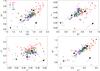 |
Fig. 6 Color−color diagrams discussed in the text. We use the color measurements obtained using the approach 1. The colors are corrected for Galactic extinction. The arrows indicate the reddening vectors (the length correspond to 0.1 mag extinction in the r-band). The black circle represents the mean color of the elliptical galaxies from Shimasaku et al. (2001). The black star and the black downward triangle represent the mean colors of S0−Sb and Sbc−late-type galaxies from Muñoz-Mateos et al. (2009), respectively. |
5.2. Color−color diagrams
In Fig. 6 the color−color diagrams are plotted showing the central peaks (red asterisks), barlenses (pink filled circles), thin bars (green open circles), and disks (blue crosses). In the case of central peaks, only nuc1 regions are shown because nuc2 might contain contamination from the colors of nuclear rings. In the two upper panels plotted are (g−r) vs. (u−g), and (r−i) vs. (g−r), whereas in the lower panels (i−z) vs. (r−i) and (g−i) vs. (u−r) are shown. As a comparison we also plotted the mean values for the elliptical galaxies (black circle) in Shimasaku et al. (2001) and the S0/a−Sb (black star) and Sbc-late-type galaxies (black downward triangle) in Muñoz-Mateos et al. (2009), shown in Table 3.
Photometric separations of the stellar populations in these color bands were discussed for example by Fukugita et al. (1996) and Lenz et al. (1998). In all the color−color diagrams the reddening vectors are also shown. In Fig. 7 the tracks of the stellar evolutionary models are shown in the same diagrams, and also the mean values for the different types of galaxies from the literature as in Fig. 6. The models are from Bruzual & Charlot (2003), using their “Padova 1994” evolutionary tracks, the Chabrier (2003) Initial Mass Function (IMF), and STELIB spectral library (Le Borgne et al. 2003). The tracks were calculated for different stellar ages and metallicities, indicated in the figure. According to Terlevich & Forbes (2002) typical metallicities for the galaxies in Hubble types of S0−Sa are between [Fe/H] = −0.45−0.50.
Between the u and g bands the stellar spectra contain the Balmer jump, which is sensitive to stellar surface gravity. Therefore the first diagram (upper left panel) is good for separating the main sequence stars from giant stars. As most of the line-blanketing from heavy elements occurs at short wavelengths, among the selected diagrams this is perhaps also the most sensitive to metallicity. In the Fig. 3 by Lenz et al. (1998), for a given (g−r) color the more metal rich stars have a higher (u−g) color index. The second diagram (upper right panel) separates the stars according to their effective temperatures in a more clear manner, although metallicity also still plays some role. At the color range useful in this study, the third diagram (lower left panel) is at some level also sensitive to the metallicity of giants stars. The (u−r) color index in the forth diagram (lower right panel) is sensitive to short lived stars, in a similar manner as the equivalent width of Hα (EW(Hα)) (see Casado et al. 2015).
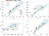 |
Fig. 7 Stellar evolutionary models of Bruzual & Charlot (2003) are calculated to four different metallicities, for the range of stellar ages of 1−20 Gyr. The models use their “Padova 1994” evolutionary tracks, the Chabrier (2003) Initial Mass Function (IMF), and STELIB spectral library (Le Borgne et al. 2003). The tracks are calculated for the same color indices as the observations shown in Fig. 6, and the black symbols represent the same galaxy samples as before. The ranges spanned by our observations are marked with the hatched regions. |
(g−r) vs. (u−g):
The bar components are mostly distributed to a narrow range of (g−r) colors of ~0.7−0.8, indicating that they are dominated by K-giant stars. Overall the colors of the two bar components (barlens and thin bar) fall into the same region in this diagram. Therefore, taking into account that this diagram is also the most sensitive to metallicity means that the metallicities of the two bar components must be similar. On the other hand, the central regions of the galaxies (i.e., nuc1) are shifted to (g−r) > 0.8 and (u−g) > 1.8. For these high values of (g−r) and (u−g) colors the age-metallicity degeneracy prevents of making any conclusions of their possible higher metallicities or older ages. Simply high extinction in the central regions could explain the observed colors. Also a large majority of the disks have similar colors as bars in this diagram, but there are also some galaxies in which the disks are shifted to bluer colors: however even these colors (g−r> 0.6) are representative of stellar populations dominated by K-giant stars.
(r−i) vs. (g−r):
Also in this diagram the two bar components have very similar colors. However, the colors of the central peaks and the disks deviate from those of bars: for a given (r−i) the (g−r) color is redder for the central regions and bluer for the disks. As the reddening vector goes nearly perpendicular to the obtained shifts between the different structure components, the shifts cannot be explained by internal galactic extinction. Based on the simple models in Fig. 7 the shifts are not due to metallicity either. It is possible that the model tracks use too simple model for star formation and therefore cannot account the observations well.
(i−z) vs. (r−i):
Again, the two bar components have very similar colors, whereas the central peaks and disks are shifted so that for a given (r−i) color the central peaks have redder (i−z) color, and the disks have bluer color. According to Shimasaku et al. (2001) there is 0.1−0.2 mag uncertainty in the z-band calibration of the SDSS images, but that is not critical in this study because we are looking at the relative colors between the structure components. Again, these color differences between the structure components cannot be explained neither by internal galactic extinction, nor by metallicity, in particular if solar or super-solar metallicities are concerned. Obviously, the central peaks are more dominated by the infrared flux observed in the z-band, whereas the bars and disks are less dominated by the infrared flux.
(g−i) vs. (u−r):
The last panel uses (u−r) which is sensitive to the presence of massive, short-lived stars that dominate the blue part of the spectrum (Casado et al. 2015). The color index (u−r) traces stellar populations ages not much older than OB stars, traced by EW(Hα). Based on the studies of a large galaxy sample and using the SDSS images, it has been shown that the division line between active and passive galaxies appears at (u−r) = 2.3 (Casado et al. 2015; McIntosh et al. 2014). This also marks the well known red and blue sequence among the galaxies in the Hubble sequence. Looking at our Fig. 6 (lower right panel) it appears that all the structure components studied by us are mostly passive. The central peaks are even redder than the bars or disks, having (u−r) = 2.5−3.0. However, among all the structures there are some individual cases in which manifestations of active star formation appears (u−r< 2.3).
In conclusion: thin bars and barlenses have similar colors. The main body of them have colors best traced with the stellar evolutionary tracks with stellar ages of 5−10 Gyr and solar metallicity (Z0), mainly in the (g−r) vs. (u−g) and (g−i) vs. (u−r) color−color diagrams. However, the colors are not so well accounted when (r−i) appears in the diagram, which leaves uncertain the interpretation of the color−color plots using (r−i). In any case, taking into account the reddening vectors it is clear that extinction alone cannot explain the redder central colors. Using nuc2 instead of nuc1 would reduce the difference between the central regions and barlenses, because possible central star forming rings are then covered. However, even the central regions appear redder than barlenses.
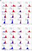 |
Fig. 8 Color differences between the structure components calculated separately for each galaxy. Shown are the histograms of the deviations from barlens color (blc), for the color subsample. The deviations are shown in four color indices. The red and blue colors indicate whether the deviations are toward redder or bluer color, when compared to the color of the barlens. The numbers are the median values of the deviations, indicated also by the vertical lines, and the standard deviations (σ). Panel a) uses the measurements from approach 1 and panel b) those from approach 2 (see Sect. 4.2). The estimated photometric accuracy of the colors of individual galaxies is 0.03 mag. |
5.3. Comparison of the colors of barlenses with respect to those of the other structure components
In the following the colors of the structure components are derived galaxy by galaxy. In each color we calculated how much the barlens color deviates from the color of another component, that is, from the central peak, the thin bar, or the disk. These color differences are shown in Fig. 8 using the same color indices as above. In the histograms positive and negative deviations are shown with red and blue colors, respectively. The median values of the color differences are also indicated in the plots. The measurements using the two approaches explained in Sect. 4.2 are shown in panels a and b.
This analysis also shows that the colors of barlenses are very similar to the colors of the thin bars of the same galaxies, manifested as almost zero deviations in their average color differences. Small deviations to both directions appear particularly in (u−g) and (g−r), which can be associated to metallicity, star formation, or small differences in the dominant stellar populations. This is not unexpected having in mind that some of the barlenses have rich structures manifested in their color maps, as will be shown in the next section.
The central peaks (nuc1) are systematically redder than barlenses in all the color indices except in (r−i). Using the larger apertures (nuc2) gives somewhat bluer relative colors, because in some of the galaxies the central color is contaminated by a star forming nuclear ring. Anyway, the obtained tendencies for the colors of the central regions is independent of the aperture size used. However, there are also some barlenses in which the central region is clearly bluer than the barlens, which is manifested particularly in (u−g) and (g−r), and a hint of that appears also in (r−i). In (r−i) this might be related to prominent emission lines in star forming regions in r-band. On the other hand, the colors of the disks within the bar radii are systematically bluer than those of barlenses. Again, this is the case in all the other colors except in (r−i).
5.4. Color profiles of individual galaxies
Color profiles in (g−r) and (i−z) for the barlens galaxies in our color subsample are shown in Fig. 9 and Appendix B. The color profiles were obtained from the corresponding color map, along the bar major axis, within the stripes shown in Fig. 10 (region between two parallel dashed lines). The stripes were defined to have a width of 0.2 × rbl centered on the galaxy center. What is actually shown in the profiles are the color deviations in respect of the median colors along the bar major-axis. The radial coordinates are normalized to rbar.
The color profiles were divided into groups based on how flat the profiles are. F indicates a completely flat color profile in which any deviation from flatness is not larger than the random color variations of the profile. RP indicates that the galaxy has a red central peak which is clearly larger than the random variations. RP+nr includes galaxies that have a red central peak and also a nuclear ring clearly identifiable as two minima in the (g−r) color profile, one at each side of the peak. nb contains galaxies with nuclear bars classified by Buta et al. (2015). B contains barlenses with bluer nuclear features due to a nuclear ring or a blue central peak, here the (g−r) profile shows a minimum in the central region. D means that the color images show plenty of dust features inside the barlens manifested in the profiles as variable color. According to this division of the barlens galaxies to different groups, red central peaks appear in 21 (45%) of the galaxies. This number includes also the five (11%) red nuclear bars, and the five (11%) galaxies with star forming nuclear rings surrounding the red central peaks (in Appendix B: RP, RP+nr, nb). In ten (21%) of the galaxies the profiles are completely flat, and seven (15%) galaxies have blue central peaks. In nine (19%) of the galaxies the whole barlens regions are full of dust and star forming regions. The galaxies with star forming nuclear rings or red nuclear bars are indicated in Table 1. Negative color gradients in barlenses appear at least in IC 1067 and NGC 2968, and variable colors in some other galaxies, associated to complex dusty structures within the barlenses. NGC 6014 represents a particular case in which a nuclear ring is manifested as two minima in the (g−r) profile, however it shows signs of a bluer central region. We have included this galaxy in the B group (Appendix B) but considered its nuclear ring in Table 1.
In conclusion: although the small central regions of barlenses have on average redder colors than the rest of the barlens, the color profiles along the bar major axis hint to clearly red central peaks only in ~23% of the barlenses (those that belong to the RP group).
In order to characterize the extension of the red central peaks, we looked at those galaxies for which the FWHM of the images is clearly smaller than the radial extension of the peak (see Appendix B). In such cases one can be sure that the observed structure is resolved and the size can be estimated in a reliable manner. Visual inspection of the color profiles revealed that the peak extension is typically ~10% that of the bar. However, it should be kept in mind that extinction by dust can also affect this estimation of the peak extension.
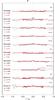 |
Fig. 9 Bar major axis color profiles in (g−r) (black) and (i−z) (red) for the barlens galaxies in the F group. The radial coordinate is normalized to the radius of the bar (rbar), and the thick lines indicate the region inside the radius of the barlens (rbl). The horizontal lines indicate the median color along the bar, and the individual profiles are shifted by 0.5 mags. The dashed vertical line indicates the galaxy center. The labels in the left give the median (g−r) and (i−z) colors, and the bar on the right represents the FWHM of the g-band image for each galaxy. Similar plots for the RP, RP+nr, nb, B and D groups are shown in Appendix B. |
Compared to the Atlas of Images of NUclear Rings (AINUR, Comerón et al. 2010) we have also detected blue nuclear rings in NGC 3185, NGC 3351, NGC 4245, and NGC 4314, which belong to our RP+nr group. On the other hand, nuclear rings are reported in AINUR for the galaxies NGC 936 and NGC 4262, classified by us as having flat color profiles. In fact, for NGC 4262 a nuclear ring might appear also in our color profile, but the signature is not very strong. In total, we have 24 galaxies in common with AINUR but only 12 of them have the full set of optical images used here (NGC 4593 has only g-band imaging). Apart from the two F and four RP+nr cases mentioned above, from AINUR we have classified one Rp (NGC 4371), two nb (NGC 2859 and NGC 4340), one B (NGC 3945), and two D (NGC 4448 and NGC 4579) as can be seen in Fig. 9 and Appendix B.
About 20% (15) of the barlens galaxies in our sample are shown to have some type of nuclear activity in HYPERLEDA (Makarov et al. 2014), being mainly Seyfert 2 nuclei or LINERs. Only NGC 4639 has Seyfert 1 type nucleus in our color subsample. However, the galaxies with nuclear activity do not show any peculiarities in their central colors. Eight of these galaxies belong to our color subsample. We have compared their nuc1 median colors with those of the rest of galaxies without active galactic nuclei (AGN) classification. The differences are Δ(u−g) = 0.024, Δ(g−r) = 0.016, Δ(r−i) = 0.034, and Δ(i−z) = 0.013 mag. These differences are smaller than, for example, those among the disks and the bars of galaxies, except in the (r−i) index (see Sect. 5.1.2). This suggests that the central parts of barlens galaxies with and without AGN are rather similar.
5.5. Color maps of individual galaxies
Color maps of the representative examples of barlens galaxies are shown in Fig. 10. The g-band images, (g−r) and (i−z) color maps, as well as the color profiles along the major and minor axes of the bar in both colors are shown. In order to facilitate the interpretation of the profiles, the images were rotated so that the bar major axis appears always horizontally. In the color profiles, the red and blue vertical lines indicate the sizes of barlenses and the thin bars, respectively. The selected galaxies are examples of the different categories shown in Fig. 9 and Appendix B, marked in parenthesis below. The colors of bars are generally fairly smooth, although some of the bars have a lot of fine-structure, related to dust extinction and recent star formation, or separate structure components like nuclear bars or star forming nuclear rings appear.
NGC 5701 (F): is an S0/a galaxy, at an inclination of inc = 15.2°. The color profiles both along the bar major and minor axes are completely flat, and the barlens shows no structure in the optical colors. The median colors are (g−r) ~ 0.77 and (i−z) ~ 0.27, which are also normal colors of elliptical galaxies according to Shimasaku et al. (2001).
NGC 4596 (RP): is an S0/a galaxy with inclination of inc = 35.5°. This galaxy has a red central peak at r ~ 5′′, which has colors of (g−r) = 0.91 and (i−z) = 0.39. At (g−r) this is a typical color of an elliptical galaxy (compared with 0.83 ± 0.14 in Shimasaku et al.), and at (i−z) slightly redder than the mean value (compared with 0.27 ± 0.06 in Shimasaku et al.). The barlens is featureless even at (g−r) color showing very little intermediate aged star formation or features of dust. This is an example of galaxies in which small classical bulges might be present in the central regions.
NGC 4314 (RP+nr): has a Hubble stage Sa, and has an inclination inc = 20.4°. This is an example of barlens galaxies which have a red central peak in the color profile along the bar major axis (in g−r and i−z). The central peak appears within r = 5′′, and has colors of (g−r)~ 0.92 and (i−z) ~ 0.35, which are redder than the mean values in normal elliptical galaxies. The red peak is surrounded by a star forming nuclear ring visible in (g−r). Outside the nuclear ring spiral arms appear, which are red in (g−r) probably being a manifestation of dust. The nuclear ring and the nuclear bar of this galaxy have been previously discussed in the optical by Erwin & Sparke (2003, see references there), and in the infrared by Laurikainen et al. (2011). In Laurikainen et al. (2014, see their Fig. 1) the observed surface brightness profiles along the bar major and minor axis were shown and compared with those predicted by the simulation model by Athanassoula et al. (2013). They concluded that these profiles are similar to those predicted by the simulation models.
NGC 4143 (nb): this is an S0 galaxy with an inclination of inc = 43.8°. It hosts a nuclear bar with a radius of rnb = 2′′ (Laurikainen et al. 2011). Looking at its (i−z) color profiles, it seems likely that the observed central peak is related to this feature. This is suggested by the peaked radial extension, which roughly corresponds to that of the nuclear bar. This can also be seen in Appendix B, given that rnb, normalized to the size of the main bar (rbar) is ~0.1, which is roughly the same extension of the central peak. However, in this case the central peak is unresolved because the FWHM is larger than the peak extension.
NGC 3380 (B): this galaxy has Hubble stage S0/a and galaxy inclination of inc = 20.8°. Belonging to category B, the barlens has a blue central region within a few arcseconds inside a redder barlens. The blue nucleus within a few arcseconds appears in both colors, but it is particularly clear in (g−r), indicating that it consists of younger stellar populations than the barlens. The bar is blue in its outskirts, and in the zone where it crosses the surrounding ring-like structure (rs).
NGC 4579 (D): this is an Sa galaxy at inc = 41.6°. This is an example of a dusty barlens galaxies. Particularly in the (g−r) color map a lot of fine structure appears inside the barlens. The star forming regions inside the barlens are oriented along the disk, but they are much more elongated than the outer disk, meaning that they are clearly associated to the barlens morphology. In the (i−z) color profile there is a small red central peak. The minor-axis profile further illustrates that the red color is associated to the whole barlens, which color steadily turns bluer from the galaxy center toward the edge of the barlens.
 |
Fig. 10 Examples of the different types of barlenses discussed in the text. For each galaxy shown are: g-band image (left), (g−r) color map (middle), and (i−z) color map (right). For the color maps shown are also the color profiles along the bar major and minor axes, measured within the regions marked with dashed lines. The vertical lines in the profiles indicate the bar (blue) and the barlens (red) radii. All the dimensions are in arcseconds, and the images are rotated so that the bar (measured from the 3.6 or 2.2 μm image) is horizontally oriented. Similar plots for the rest of galaxies in the color subsample are shown in Appendix A. |
6. Discussion
6.1. Barlenses form part of the bar
One of the main motivations of this study was to answer the question whether the optical broadband colors support the idea that barlenses form part of the bar, in a similar manner as the boxy/peanut bulges do. We have shown that the mean colors of the two bar components, barlenses and the thin bar, are identical. The colors of the two bar components also fall into the same regions in the color−color diagrams studied by us, which means that they must have fairly similar metallicities, dust content, and dominant stellar populations. However, one must keep in mind that the straight comparison of measured colors with those predicted by models provides no clear, unambiguous age information. If we look at the individual galaxies and the obtained color differences between the two bar components we end up with the same conclusion: no systematic deviations either to redder or bluer colors appear in any of the color indices. The range of deviations is extremely narrow in (r−i) and (i−z), and somewhat broader in (u−g) and (g−r). Obviously some of the barlenses are dusty and have a variable contribution of young and intermediate aged stars, which naturally explains the broadening. Our method for obtaining the colors is robust, and does not depend on whether the region of the thin bar within the barlens radius is included to the color measurement or not. So the answer is that the colors obtained for the two bar components in this study indeed are consistent with the idea that barlenses form part of the bar. The main body of the stars in barlenses were formed at the same time with the stars of the thin bars. Whether the barlens structure also formed at the same time with the rest of the bar is a matter of making detailed dynamical models for these galaxies.
The colors do not answer the question whether barlenses are also thick in the vertical direction. However, support for the vertical thickening of barlenses comes from our analysis of their apparent isophotal orientations with respect to the thin bars and the disks line-of-nodes. A comparison with the predictions of the theoretical models also provide some insight to this question. Formation of barlenses in the simulation models have been discussed by Athanassoula et al. (2015). Their simulations use GADGET-3, combining stellar N-body with SPH methods, which makes possible to model star formation during the formation and evolution of the bar. In these models the vertically thick inner bar components are protruded from the disk material soon after the bar forms. In the edge-on view they are boxy/peanuts or X-shapes structures, and in face-on view have the appearance of barlenses. No bulges were added to these models while starting the simulations, while a central concentration could grow during the simulation via bar induced gas inflow and star formation. More details of these models are explained by Athanassoula et al. (2013). For several galaxies in our sample (NGC 1022, NGC 1512, NGC 4314, NGC 4608, and NGC 5101) Athanassoula et al. (2015) suggested that the Ks-band or 3.6 μm profiles along the bar major axis can be explained by their models without invoking any assumption of a pre-existing classical bulge. Direct comparisons with the model profiles were done for NGC 5101 in Athanassoula et al. (2015, their Fig. 3 and for NGC 4314 in Laurikainen et al. (2014, their Fig. 1. They observed that the surface brightness profile along the bar minor axis is exponential. Along the bar major axis the profile is less steep and has an exponential subsection associated to the barlens. Similar bar profiles were obtained in the models by Athanassoula et al. although they were not specific models to those galaxies.
Although no predictions of specific colors of the structure components are given in these models, they do predict that the oldest stars in the vertically thin and thick bar components should have similar ages. When bars evolve in their models they are rejuvenated by later gas accretion and star formation which can be manifested throughout the bar. This is in a qualitative agreement with the similar colors obtained for the two bar components in this study, although the colors still leave open the question what are actually the ages of the oldest stars in these structures. Many of the barlenses in our sample also have rejuvenated stellar populations and strong features of dust, indicating that they have accreted gas also after the bar formation, of which gas only some fraction has ended up to the central regions of these galaxies.
6.2. Classical bulges embedded in barlenses?
Bulges in S0s are generally thought to be massive, although multi-component structural decompositions have reduced the mass estimates (Laurikainen et al. 2005, 2010, 2014; Erwin et al. 2015). However, we would still expect to see the most massive classical bulges in the S0s. Having this in mind the different groups of the barlens color profiles studied in this work are interesting. A typical profile type is flat along the bar major axis, showing no evidence of a massive (classical) bulge redder than the bar itself. In one of the barlens groups the barlens is even covered by irregular dusty features, of which NGC 2968 and NGC 1022 are good examples. Such dust features might be manifestations of ongoing gas accretion to the barlenses. In the rest of the barlens groups the characteristic features appear in the central regions of the galaxies, either associated directly with recent star formation, or manifesting themselves in the form of small red central peaks. In one the groups the red central peaks are due to red nuclear bars, but there are also barlenses in which the red central peaks are rather unresolved dusty nuclei, or small central concentrations of the old stellar populations.
Our study does not support the idea that massive classical bulges appear in S0s, but it does not rule out the possibility that small bulges other than barlenses appear in these galaxies. As colors alone are not sufficient to distinguish stellar population ages, detailed stellar population analysis for individual galaxies, combined with simulation models, is needed for retrieving the star formation histories of barlenses.
7. Summary and conclusions
We have analyzed a sample of 79 barlens galaxies that appear in the classification by Buta et al. (2015) in the Spitzer Survey of Stellar Structure in Galaxies (S4G; Sheth et al. 2010), and in the NIRS0S by Laurikainen et al. (2011). The infrared images of these surveyswere used to measure the sizes and orientations of barlenses. The conclusions made from the study of these parameters are the following:
Barlens orientations were compared with the orientations of the thin bars and the lines-of-nodes. We showed that the region where barlens galaxies appear in the |PAbar− PAdisk | vs. |PAbl− PAdisk | plane is as expected if they were vertically thick components embedded in a flat disk. In galaxies seen in nearly face-on view (inc< 40°) barlenses are often aligned with the thin bar indicating small intrinsic elongation along the thin bar.
The size and orientation measurements of barlenses obtained in this study are consistent with those previously made by Herrera-Endoqui et al. (2015) for the same galaxies.
For a subset of 47 galaxies optical colors using the Sloan Digital Sky Survey (SDSS) images at u, g, r, i, and z-bands from Knapen et al. (2014), were studied. The colors of the different structure components, including the two bar components (barlens and thin bar), the disks, and the central regions of the galaxies were measured. Color maps and color−color diagrams were also constructed. Based on the color profiles along the bar major axis, the galaxies were divided into different groups. The following conclusions were made:
Barlenses vs. thin bars: the two bar components were found to have very similar colors in all the color index images studied here. It means that their stellar populations, metallicities, and the values of internal galactic extinction must on average be fairly similar. Thus, the very similar colors that we found for the barlenses and the thin bars, are a manifestation that barlenses indeed form part of bars, in a similar manner as boxy/peanut bulges. The mean colors at (u−g), (g−r), (r−i) and (i−z) are also similar to the mean colors of normal elliptical galaxies. Galaxy by galaxy studies further showed that galaxies which have irregular features related to rejuvenated stellar populations in barlenses do exist.
Barlenses vs. central peaks: except for the (r−i) color index, the central peaks are slightly shifted toward redder colors in all of our color−color diagrams. This can be due to internal galactic extinction or higher metallicities, but based on the stellar population grids used by us no unambiguous explanations for these redder colors could be obtained. Many of the barlenses (11, accounting for ~23% of the color subsample) also have central star forming nuclear rings or redder nuclear bars.
Barlenses vs. the underlying disks: disks are systematically bluer than bars (or barlenses) in all the color indices studied here, except in (r−i). The difference is best visible in the color−color diagrams (r−i) vs. (g−r) and (i−z) vs. (r−i).
The NASA/IPAC Extragalactic Database (NED) is operated by the Jet Propulsion Laboratory, California Institute of Technology, under contract with the National Aeronautics and Space Administration.
IRAF is distributed by the National Optical Astronomy Observatories, which are operated by the Association of Universities for Research in Astronomy, Inc., under cooperative agreement with the National Science Foundation.
These equations are found in the SDSS webpage containing transformations between SDSS magnitudes and other systems: www.sdss.org/dr8/algorithms/sdssUBVRITransform.php
Acknowledgments
The authors thank the anonymous referee for comments that improved this paper. The authors acknowledge financial support from to the DAGAL network from the People Programme (Marie Curie Actions) of the European Union’s Seventh Framework Programme FP7/2007−2013 under REA grant agreement number PITN-GA-2011-289313. Special acknowledgment for the S4G-team (PI Kartik Sheth) for making this database available for us. We also acknowledge NTT at ESO, as well as NOT and WHT in La Palma, where the Ks-band images used in this study were originally obtained. E.L. and H.S. acknowledge financial support from the Academy of Finland. J.H.K. acknowledges financial support from the Spanish Ministry of Economy and Competitiveness (MINECO) under grant number AYA2013-41243-P, and thanks the Astrophysics Research Institute of Liverpool John Moores University for their hospitality, and the Spanish Ministry of Education, Culture and Sports for financial support of his visit there, through grant number PR2015-00512. M.H.E. also acknowledges Santiago Erroz Ferrer, Sébastien Comerón and Simón Díaz García for useful discussions.
References
- Athanassoula, E. 2005, MNRAS, 358, 1477 [NASA ADS] [CrossRef] [Google Scholar]
- Athanassoula, E., & Beaton, R. L. 2006, MNRAS, 370, 1499 [NASA ADS] [CrossRef] [Google Scholar]
- Athanassoula, E., Machado, R. E. G., & Rodionov, S. A. 2013, MNRAS, 429, 1949 [NASA ADS] [CrossRef] [Google Scholar]
- Athanassoula, E., Laurikainen, E., Salo, H., & Bosma, A. 2015, MNRAS, 454, 3843 [NASA ADS] [CrossRef] [Google Scholar]
- Balcells, M., & Peletier, R. F. 1994, AJ, 107, 135 [NASA ADS] [CrossRef] [Google Scholar]
- Bergvall, N., Zackrisson, E., & Caldwell, B. 2010, MNRAS, 405, 2697 [NASA ADS] [Google Scholar]
- Bettoni, D., & Galletta, G. 1994, A&A, 281, 1 [NASA ADS] [Google Scholar]
- Bruzual, G., & Charlot, S. 2003, MNRAS, 344, 1000 [NASA ADS] [CrossRef] [Google Scholar]
- Bureau, M., Aronica, G., Athanassoula, E., et al. 2006, MNRAS, 370, 753 [NASA ADS] [CrossRef] [Google Scholar]
- Buta, R. J., Sheth, K., Athanassoula, E., et al. 2015, ApJS, 217, 32 [NASA ADS] [CrossRef] [Google Scholar]
- Casado, J., Ascasibar, Y., Gavilán, M., et al. 2015, MNRAS, 451, 888 [NASA ADS] [CrossRef] [Google Scholar]
- Chabrier, G. 2003, PASP, 115, 763 [NASA ADS] [CrossRef] [Google Scholar]
- Combes, F., Debbasch, F., Friedli, D., & Pfenniger, D. 1990, A&A, 233, 82 [NASA ADS] [Google Scholar]
- Comerón, S., Knapen, J. H., Beckman, J. E., et al. 2010, MNRAS, 402, 2462 [NASA ADS] [CrossRef] [Google Scholar]
- Elmegreen, B. G., & Elmegreen, D. M. 1985, ApJ, 288, 438 [NASA ADS] [CrossRef] [Google Scholar]
- Erwin, P., & Sparke, L. S. 2003, ApJS, 146, 299 [NASA ADS] [CrossRef] [Google Scholar]
- Erwin, P., & Debattista, V. P. 2013, MNRAS, 431, 3060 [NASA ADS] [CrossRef] [Google Scholar]
- Erwin, P., Saglia, R. P., Fabricius, M., et al. 2015, MNRAS, 446, 4039 [NASA ADS] [CrossRef] [Google Scholar]
- Fazio, G. G., Hora, J. L., Allen, L. E., et al. 2004, ApJS, 154, 10 [NASA ADS] [CrossRef] [Google Scholar]
- Fisher, D. B., & Drory, N. 2016, in Galactic Bulges, eds. E. Laurikainen, R. Peletier, & D. Gadotti (Springer International Publishing), Astrophys. Space Sci. Lib., 418, 41 [Google Scholar]
- Fukugita, M., Ichikawa, T., Gunn, J. E., et al. 1996, AJ, 111, 1748 [NASA ADS] [CrossRef] [Google Scholar]
- Gadotti, D. A., & de Souza, R. E. 2006, ApJS, 163, 270 [NASA ADS] [CrossRef] [Google Scholar]
- Gunn, J. E., Carr, M., Rockosi, C., et al. 1998, AJ, 116, 3040 [NASA ADS] [CrossRef] [Google Scholar]
- Herrera-Endoqui, M., Díaz-García, S., Laurikainen, E., & Salo, H. 2015, A&A, 582, A86 [NASA ADS] [CrossRef] [EDP Sciences] [Google Scholar]
- Kennicutt, Jr., R. C. 1992, ApJS, 79, 255 [NASA ADS] [CrossRef] [Google Scholar]
- Knapen, J. H., Erroz-Ferrer, S., Roa, J., et al. 2014, A&A, 569, A91 [NASA ADS] [CrossRef] [EDP Sciences] [Google Scholar]
- Kormendy, J. 1983, ApJ, 275, 529 [NASA ADS] [CrossRef] [Google Scholar]
- Kormendy, J. 2016, in Galactic Bulges, eds. E. Laurikainen, R. Peletier, & D. Gadotti (Springer International Publishing), Astrophys. Space Sci. Lib., 418, 431 [Google Scholar]
- Kurucz, R. L. 1991, in Precision Photometry: Astrophysics of the Galaxy, eds. A. G. D. Philip, A. R. Upgren, & K. A. Janes, 27 [Google Scholar]
- Laurikainen, E., & Salo, H. 2016, in Galactic Bulges, eds. E. Laurikainen, R. Peletier, and D. Gadotti (Springer International Publishing), Astrophysics Space Sci. Lib., 418, 77 [NASA ADS] [CrossRef] [Google Scholar]
- Laurikainen, E., Salo, H., & Buta, R. 2005, MNRAS, 362, 1319 [NASA ADS] [CrossRef] [Google Scholar]
- Laurikainen, E., Salo, H., Buta, R., Knapen, J. H., & Comerón, S. 2010, MNRAS, 405, 1089 [NASA ADS] [Google Scholar]
- Laurikainen, E., Salo, H., Buta, R., & Knapen, J. H. 2011, MNRAS, 418, 1452 [NASA ADS] [CrossRef] [Google Scholar]
- Laurikainen, E., Salo, H., Athanassoula, E., Bosma, A., & Herrera-Endoqui, M. 2014, MNRAS, 444, L80 [NASA ADS] [CrossRef] [Google Scholar]
- Le Borgne, J.-F., Bruzual, G., Pelló, R., et al. 2003, A&A, 402, 433 [NASA ADS] [CrossRef] [EDP Sciences] [Google Scholar]
- Lenz, D. D., Newberg, J., Rosner, R., Richards, G. T., & Stoughton, C. 1998, ApJS, 119, 121 [NASA ADS] [CrossRef] [MathSciNet] [Google Scholar]
- Lütticke, R., Dettmar, R.-J., & Pohlen, M. 2000, A&AS, 145, 405 [NASA ADS] [CrossRef] [EDP Sciences] [Google Scholar]
- Makarov, D., Prugniel, P., Terekhova, N., Courtois, H., & Vauglin, I. 2014, A&A, 570, A13 [Google Scholar]
- McIntosh, D. H., Wagner, C., Cooper, A., et al. 2014, MNRAS, 442, 533 [NASA ADS] [CrossRef] [Google Scholar]
- Méndez-Abreu, J., Corsini, E. M., Debattista, V. P., et al. 2008, ApJ, 679, L73 [NASA ADS] [CrossRef] [Google Scholar]
- Méndez-Abreu, J., Debattista, V. P., Corsini, E. M., & Aguerri, J. A. L. 2014, A&A, 572, A25 [NASA ADS] [CrossRef] [EDP Sciences] [Google Scholar]
- Muñoz-Mateos, J. C., Gil de Paz, A., Zamorano, J., et al. 2009, ApJ, 703, 1569 [NASA ADS] [CrossRef] [Google Scholar]
- Muñoz-Mateos, J. C., Sheth, K., Regan, M., et al. 2015, ApJS, 219, 3 [NASA ADS] [CrossRef] [Google Scholar]
- Okamura, S., & Takase, B. 1976, Ap&SS, 41, 275 [NASA ADS] [CrossRef] [Google Scholar]
- Pfenniger, D., & Friedli, D. 1991, A&A, 252, 75 [NASA ADS] [Google Scholar]
- Pohlen, M., & Trujillo, I. 2006, A&A, 454, 759 [NASA ADS] [CrossRef] [EDP Sciences] [Google Scholar]
- Raha, N., Sellwood, J. A., James, R. A., & Kahn, F. D. 1991, Nature, 352, 411 [NASA ADS] [CrossRef] [Google Scholar]
- Salo, H., Laurikainen, E., Laine, J., et al. 2015, ApJS, 219, 4 [NASA ADS] [CrossRef] [Google Scholar]
- Schlafly, E. F., & Finkbeiner, D. P. 2011, ApJ, 737, 103 [NASA ADS] [CrossRef] [Google Scholar]
- Schlegel, D. J., Finkbeiner, D. P., & Davis, M. 1998, ApJ, 500, 525 [NASA ADS] [CrossRef] [Google Scholar]
- Sheth, K., Regan, M., Hinz, J. L., et al. 2010, PASP, 122, 1397 [NASA ADS] [CrossRef] [Google Scholar]
- Shimasaku, K., Fukugita, M., Doi, M., et al. 2001, AJ, 122, 1238 [NASA ADS] [CrossRef] [Google Scholar]
- Terlevich, A. I., & Forbes, D. A. 2002, MNRAS, 330, 547 [NASA ADS] [CrossRef] [Google Scholar]
- Weiland, J. L., Arendt, R. G., Berriman, G. B., et al. 1994, ApJ, 425, L81 [NASA ADS] [CrossRef] [Google Scholar]
- Williams, M. J., Bureau, M., & Kuntschner, H. 2012, MNRAS, 427, L99 [NASA ADS] [Google Scholar]
- York, D. G., Adelman, J., Anderson, Jr., J. E., et al. 2000, AJ, 120, 1579 [Google Scholar]
Appendix A: Color maps and color profiles of the barlens galaxies in the color subsample
In this Appendix we include similar plots as those presented in Fig. 10 for the complete barlens color subsample. For each galaxy we show the g-band image in the bar region (left panel), the (g−r) color map and color profiles both along the major and minor axes of the bar (middle panels), and the corresponding (i−z) color map and profiles (right panels).
 |
Fig. A.1 continued. |
 |
Fig. A.1 continued. |
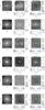 |
Fig. A.1 continued. |
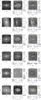 |
Fig. A.1 continued. |
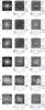 |
Fig. A.1 continued. |
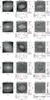 |
Fig. A.1 continued. |
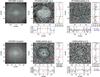 |
Fig. A.1 continued. |
Appendix B: Color profiles of the barlens galaxies in the color subsample
In this appendix we show the same information as in Fig. 9 for the RP, RP+nr, nb, B and D profile groups (see text for details).
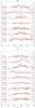 |
Fig. B.1 continued. |
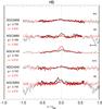 |
Fig. B.1 continued. |
Appendix C: Additional table
Sample of barlens galaxies used in this paper.
All Tables
Color index measurements for the structures of the galaxies in the color subsample.
Color indices for elliptical (Shimasaku et al. 2001) and SINGS galaxies (Muñoz-Mateos et al. 2009).
All Figures
|
Fig. 1 Example barlens galaxy, NGC 1350. Left panel: the bar region of the 3.6 μm image. Marked are the structure components measured in this study: “bl” refers to barlens, “thin bar” is the bar region outside the barlens, and “nucleus” refers to possible small bulge in the central regions. Right panel: the contours of the same image. Lines indicating the orientations of the bar (blue line), barlens (red line), and the disk line-of-nodes (dashed line) are over-plotted. Black crosses show the points selected to measure the size and orientation of the barlens by fitting an ellipse to these points. |
| In the text | |
|
Fig. 2 Distributions of morphological type, inclination, absolute B magnitude, and bar size, for the whole sample of barlens galaxies (green histogram), and for the subsample of galaxies with SDSS imaging (blue histogram). The green solid and blue dashed vertical lines show the median values of the distributions for the complete and color subsample, respectively. |
| In the text | |
|
Fig. 3 Sizes (rbl), axial ratios ((b/a)bl) and position angles (PAbl) of barlenses obtained in this study are compared with those previosuly obtained by Herrera-Endoqui et al. (2015) or Laurikainen et al. (2011). Dotted lines indicate linear fits between the old and new measurements, whereas the dashed line stands for a unit slope. The labels indicate the slope and correlation coefficient of the linear fit. The galaxies that belong to the color subsample are indicated with an open symbol. |
| In the text | |
|
Fig. 4 Orientations of barlenses compared with the orientations of bars and those of the lines-of-nodes (disks). The y-axis is the difference between the orientations of the barlens and the disk, whereas the x-axis is the difference between the orientations of the bar and the disk. The differences are given in degrees. Shown are only galaxies where the barlens axial ratio (b/a)bl< 0.9. The galaxies that belong to the color subsample are indicated with an open symbol. |
| In the text | |
|
Fig. 5 Illustration of the two methods used for defining the regions for the measurements of the component colors. In the left panel the r-band image of NGC 4245 is shown. In the middle panel we show the automatically defined regions for the central region (“nuc1” and “nuc2”; light and dark blue, respectively), for the barlens (“blc”; red), the bar (green), and the disk (yellow), see the text for details. In the right panel the manually selected regions for the barlens, the bar and the disk are shown (central regions are the same as in the middle panel). All images are in the same scale. |
| In the text | |
|
Fig. 6 Color−color diagrams discussed in the text. We use the color measurements obtained using the approach 1. The colors are corrected for Galactic extinction. The arrows indicate the reddening vectors (the length correspond to 0.1 mag extinction in the r-band). The black circle represents the mean color of the elliptical galaxies from Shimasaku et al. (2001). The black star and the black downward triangle represent the mean colors of S0−Sb and Sbc−late-type galaxies from Muñoz-Mateos et al. (2009), respectively. |
| In the text | |
|
Fig. 7 Stellar evolutionary models of Bruzual & Charlot (2003) are calculated to four different metallicities, for the range of stellar ages of 1−20 Gyr. The models use their “Padova 1994” evolutionary tracks, the Chabrier (2003) Initial Mass Function (IMF), and STELIB spectral library (Le Borgne et al. 2003). The tracks are calculated for the same color indices as the observations shown in Fig. 6, and the black symbols represent the same galaxy samples as before. The ranges spanned by our observations are marked with the hatched regions. |
| In the text | |
|
Fig. 8 Color differences between the structure components calculated separately for each galaxy. Shown are the histograms of the deviations from barlens color (blc), for the color subsample. The deviations are shown in four color indices. The red and blue colors indicate whether the deviations are toward redder or bluer color, when compared to the color of the barlens. The numbers are the median values of the deviations, indicated also by the vertical lines, and the standard deviations (σ). Panel a) uses the measurements from approach 1 and panel b) those from approach 2 (see Sect. 4.2). The estimated photometric accuracy of the colors of individual galaxies is 0.03 mag. |
| In the text | |
|
Fig. 9 Bar major axis color profiles in (g−r) (black) and (i−z) (red) for the barlens galaxies in the F group. The radial coordinate is normalized to the radius of the bar (rbar), and the thick lines indicate the region inside the radius of the barlens (rbl). The horizontal lines indicate the median color along the bar, and the individual profiles are shifted by 0.5 mags. The dashed vertical line indicates the galaxy center. The labels in the left give the median (g−r) and (i−z) colors, and the bar on the right represents the FWHM of the g-band image for each galaxy. Similar plots for the RP, RP+nr, nb, B and D groups are shown in Appendix B. |
| In the text | |
|
Fig. 10 Examples of the different types of barlenses discussed in the text. For each galaxy shown are: g-band image (left), (g−r) color map (middle), and (i−z) color map (right). For the color maps shown are also the color profiles along the bar major and minor axes, measured within the regions marked with dashed lines. The vertical lines in the profiles indicate the bar (blue) and the barlens (red) radii. All the dimensions are in arcseconds, and the images are rotated so that the bar (measured from the 3.6 or 2.2 μm image) is horizontally oriented. Similar plots for the rest of galaxies in the color subsample are shown in Appendix A. |
| In the text | |
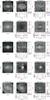 |
Fig. A.1 Same as Fig. 10. |
| In the text | |
|
Fig. A.1 continued. |
| In the text | |
|
Fig. A.1 continued. |
| In the text | |
|
Fig. A.1 continued. |
| In the text | |
|
Fig. A.1 continued. |
| In the text | |
|
Fig. A.1 continued. |
| In the text | |
|
Fig. A.1 continued. |
| In the text | |
|
Fig. A.1 continued. |
| In the text | |
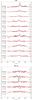 |
Fig. B.1 Same as Fig. 9. |
| In the text | |
|
Fig. B.1 continued. |
| In the text | |
|
Fig. B.1 continued. |
| In the text | |
Current usage metrics show cumulative count of Article Views (full-text article views including HTML views, PDF and ePub downloads, according to the available data) and Abstracts Views on Vision4Press platform.
Data correspond to usage on the plateform after 2015. The current usage metrics is available 48-96 hours after online publication and is updated daily on week days.
Initial download of the metrics may take a while.