| Issue |
A&A
Volume 598, February 2017
|
|
|---|---|---|
| Article Number | A50 | |
| Number of page(s) | 20 | |
| Section | Extragalactic astronomy | |
| DOI | https://doi.org/10.1051/0004-6361/201629432 | |
| Published online | 01 February 2017 | |
Supernova rates from the SUDARE VST-Omegacam search II. Rates in a galaxy sample ⋆
1 INAF–Osservatorio Astronomico di Capodimonte, Salita Moiariello 16, 80131 Napoli, Italy
e-mail: This email address is being protected from spambots. You need JavaScript enabled to view it.
2 INAF–Osservatorio Astronomico di Padova, vicolo dell’Osservatorio 5, 35122 Padova, Italy
3 Departemento de Ciencias Fisicas, Universidad Andres Bello, Santiago, Chile
4 Millennium Institute of Astrophysics, Santiago, Chile
5 International Center for Relativistic Astrophysics, Piazzale della Repubblica 2, 65122 Pescara, Italy
6 Department of Physics and Astronomy, University of the Western Cape, 7535 Bellville, Cape Town, South Africa
7 INAF – Istituto di Radioastronomia, via Gobetti 101, 40129 Bologna, Italy
8 INAF–Osservatorio Astronomico di Catania, via S. Sofia 78, 95123 Catania, Italy
9 Dipartimento di Fisica, Universitá Federico II, 80131 Napoli, Italy
10 AlbaNova University Center, KTH Royal Institute of Technology, Roslagstullsbacken 21, 106 91 Stockholm, Sweden
11 Astrophysics, University of Oxford, Denys Wilkinson Building, Keble Road, Oxford OX1 3RH, UK
12 Department of Physical Sciences, The Open University, Milton Keynes, MK7 6AA, UK
13 ASI Science Data Center, via del Politecnico snc, 00133 Roma, Italy
Received: 29 July 2016
Accepted: 2 October 2016
Abstract
Aims. This is the second paper of a series in which we present measurements of the supernova (SN) rates from the SUDARE survey. The aim of this survey is to constrain the core collapse (CC) and Type Ia SN progenitors by analysing the dependence of their explosion rate on the properties of the parent stellar population averaging over a population of galaxies with different ages in a cosmic volume and in a galaxy sample. In this paper, we study the trend of the SN rates with the intrinsic colours, the star formation activity and the masses of the parent galaxies. To constrain the SN progenitors we compare the observed rates with model predictions assuming four progenitor models for SNe Ia with different distribution functions of the time intervals between the formation of the progenitor and the explosion, and a mass range of 8−40 M⊙ for CC SN progenitors.
Methods. We considered a galaxy sample of approximately 130 000 galaxies and a SN sample of approximately 50 events. The wealth of photometric information for our galaxy sample allows us to apply the spectral energy distribution (SED) fitting technique to estimate the intrinsic rest frame colours, the stellar mass and star formation rate (SFR) for each galaxy in the sample. The galaxies have been separated into star-forming and quiescent galaxies, exploiting both the rest frame U−V vs. V−J colour−colour diagram and the best fit values of the specific star formation rate (sSFR) from the SED fitting.
Results. We found that the SN Ia rate per unit mass is higher by a factor of six in the star-forming galaxies with respect to the passive galaxies, identified as such both on the U−V vs. V−J colour−colour diagram and for their sSFR. The SN Ia rate per unit mass is also higher in the less massive galaxies that are also younger. These results suggest a distribution of the delay times (DTD) less populated at long delay times than at short delays. The CC SN rate per unit mass is proportional to both the sSFR and the galaxy mass, confirming that the CC SN progenitors explode soon after the end of the star formation activity. The trends of the Type Ia and CC SN rates as a function of the sSFR and the galaxy mass that we observed from SUDARE data are in agreement with literature results at different redshifts suggesting that the ability of the stellar populations to produce SN events does not vary with cosmic time. The expected number of SNe Ia is in agreement with that observed for all four DTD models considered both in passive and star-forming galaxies so we can not discriminate between different progenitor scenarios. The expected number of CC SNe is higher than that observed, suggesting a higher limit for the minimum progenitor mass. However, at least part of this discrepancy between expected and observed number of CC SNe may reflect a fluctuation due to the relatively poor statistics. We also compare the expected and observed trends of the SN Ia rate with the intrinsic U−J colour of the parent galaxy, assumed to be a tracer of the age distribution. While the slope of the relation between the SN Ia rate and the U−J colour in star-forming galaxies can be well-reproduced by all four DTD models considered, only the steepest of them is able to account for the rates and colour in star-forming and passive galaxies with the same value of the SN Ia production efficiency. The agreement between model predictions and data could be found for the other DTD models, but with a productivity of SN Ia higher in passive galaxies compared to star-forming galaxies.
Key words: supernovae: general / surveys / galaxies: star formation / galaxies: stellar content
Based on observations made with ESO telescopes at the Paranal Observatory under programme ID 088.D-4006, 088.D-4007, 089.D-0244, 089.D-0248, 090.D-0078, 090.D-0079, 088.D-4013, 089.D-0250, 090.D-0081.
© ESO, 2017
1. Introduction
Supernovae (SNe), dramatic and violent end-points of stellar evolution, are involved in the formation of neutron stars, black holes and gamma-ray bursts and are sources of gravitational waves, neutrino emission and high-energy cosmic rays (e.g., Heger et al. 2003; Woosley & Bloom 2006; Fryer et al. 2012).
SNe also play an important role in driving the dynamical and chemical evolution of galaxies, contributing to the feedback processes in galaxies (Ceverino & Klypin 2009), producing heavy elements and dust (e.g. Bianchi & Schneider 2007).
SNe are formidable cosmological probes due to their huge intrinsic brightness. In particular, Type Ia SNe have provided the first evidence for an accelerated expansion of the Universe (Perlmutter et al. 1998, 1999; Riess et al. 1998; Schmidt et al. 1998) and remain one of the more promising probes of the nature of dark energy (e.g., Sullivan et al. 2011; Salzano et al. 2013; Dark Energy Survey Collaboration et al. 2016).
We recognise two main, physically defined SN classes: core collapse-induced explosions (CC SNe) of short-lived massive stars (M ≳ 8 M⊙) and thermonuclear explosions (SNe Ia) of long-lived, intermediate mass stars (3 ≲ M ≲ 8 M⊙) in binary systems.
There exists a considerable range of CC SNe physical characteristics including kinetic energy, radiated energy, ejecta mass and amount of radioactive elements created during explosion. Different sub-types of CC SNe have been identified on the basis of their spectro-photometric evolution (IIP, IIL, IIn, IIb, Ib, Ic, IcBL) and have been associated to a possible sequence of progenitors related to their mass loss history, with the most massive stars and stars in binary systems losing the largest fraction of their initial mass. However, this simple scheme, where only mass loss drives the evolution of CC SN progenitors, has difficulty explaining the relative fraction of different types, as well as the variety of properties exhibited by CC SNe of the same type (e.g. Smith et al. 2011). In recent years the progenitor stars of several type IIP SNe have been detected on pre-explosion images out to 25 Mpc (Smartt 2009, and references therein), while there are few progenitors detected for IIb and Ib SNe (Bersten et al. 2012; Cao et al. 2013; Bersten et al. 2014; Eldridge et al. 2015; Fremling et al. 2016) and no progenitors for type Ic SNe. The lack of detection of red supergiant progenitors with initial masses between 17 and 30 M⊙ remains in question and several possible explanations have been suggested (Smartt 2009). Moreover, several observational evidences have suggested that a significant fraction of type Ib/c progenitors are stars of initial mass lower than 25 M⊙ in close binary systems stripped of their envelopes by the interaction with the companion (e.g., Eldridge et al. 2013).
There is a general consensus that SNe Ia correspond to thermonuclear explosions of a carbon and oxygen white dwarf (WD) reaching the Chandrasekhar mass due to accretion from a close companion. The evolutionary path that leads a WD to mass growth, ignition, and explosion is still unknown. The most widely favoured progenitor scenarios are the single degenerate scenario (SD) in which a WD, accreting from a non degenerate companion (a main sequence star, a sub-giant, a red giant or a helium star), grows in mass until it reaches the Chandrasekhar mass and explodes in a thermonuclear runaway (Whelan & Iben 1973), and the double degenerate scenario (DD), in which a close double WD system merges after orbital shrinking due to the emission of gravitational waves (Tutukov & Yungelson 1981; Iben & Tutukov 1984). Unfortunately, to date, there is no conclusive evidence from observations decisively supporting one channel over the other (e.g. Maoz et al. 2014). Actually, both channels may well contribute in comparable fractions of events (Greggio 2010), as suggested by some observational facts, yet the contribution of each channel to the overall Type Ia population is very hard to assess.
The modern SN searches discovering transients with no galaxy bias, faint limiting magnitudes, and very fast evolution are challenging the paradigms we hold for SN progenitors, suggesting an unexpectedly large range of explosion proprieties and new SN classes (e.g. Iax, Ibn or super luminous SNe). It is then of foremost importance to answer open questions with regard to SN progenitor systems, explosion mechanisms and physical parameters driving the observed SN diversity.
In this framework, the analysis of the dependence of the SN rate on the age distribution of the parent stellar population can help to constrain the progenitor scenarios and hence improve understanding of the effects of age on the SN diversity (e.g. Greggio 2010).
Due to the short lifetime of progenitor stars, the rate of CC SNe directly traces the current star formation rate (SFR) of the host galaxy. Therefore the mass range for CC SN progenitors can be probed by comparing the rate of born stars and the rate of CC SNe occurring in the host galaxy, assuming the distribution of the masses with which stars are born, that is, the initial mass function (IMF). On the other hand, the rate of SNe Ia echoes the whole star formation history (SFH) of the host galaxy due to the time elapsed from the birth of the binary system to the final explosion, referred to as delay-time. SNe Ia are observed to explode both in young and old stellar populations and the age distribution of the SN Ia progenitors is still considerably debated (e.g. Maoz et al. 2014). By comparing the observed SN Ia rate with what is expected for the SFH of the parent stellar population, it is possible to constrain the progenitor scenario and the fraction of the binaries exploding as SNe Ia (Greggio 2005; Greggio et al. 2008; Greggio 2010).
Ideally, we should compare SFH and SN rates in each individual galaxy (e.g. Maoz et al. 2012) or for each resolved stellar population in a given galaxy. To minimise the uncertainties in SN rates and SFHs based on individual galaxies we can average over a galaxy sample or in a large cosmic volume. In the first case, one estimates a characteristic average age for a sample of galaxies via morphological types, colours or spectral energy distribution (SED) fitting; in the second case, one averages over a population of galaxies with different ages and evolutionary paths, by assuming a cosmic SFH.
In order to measure SN rates both at different cosmic epochs and in a well defined galaxy sample, we started the SUpernova Diversity And Rate Evolution (SUDARE) programme ran at the VLT Survey Telescope (VST) (Botticella et al. 2013). The survey strategy, the pipeline and the estimate of SN rates in a cosmic volume are described in Cappellaro et al. (2015; hereafter Paper I). In the present paper we illustrate the measurement of SN rates for the main SN types as a function of galaxy colours, SFR, specific star formation (sSFR) and mass.
This paper is organised as follows. In Sect. 2, we describe the method that we used to estimate the properties of the galaxies monitored by SUDARE. In Sect. 3, we outline how we selected the SN sample and identified the host galaxy of each SN. In Sect. 4, we illustrate how we measured rates in our galaxy sample. Finally, we investigate how SN rates are dependent on the properties of the host galaxies: rest frame colours (Sect. 5), star-formation quenching (Sect. 6), sSFR (Sect. 7), and stellar mass (Sect. 8). A comparison of the observed rates with predictions from theoretical models is presented in Sect. 9, while our conclusions are summarised in Sect. 10. In the Appendix we present the analysis of rates for different CC SN subtypes (Appendix A) and systematic errors (Appendix B). Throughout, we assume a standard cosmology with H0 = 70 km s-1 Mpc-1, ΩM = 0.3 and ΩΛ = 0.7 and we adopt a Salpeter IMF from 0.1 to 100 M⊙ (Salpeter 1955) and the AB magnitude system (Gunn et al. 1998).
2. Galaxy properties
In order to relate the SN events and their rates to fundamental properties of their progenitors we need to characterise the stellar populations in the sample galaxies we monitored for SNe, and in particular their SFH. The latter can be derived from integrated rest-frame colours in various combinations, or, more in detail, from the galaxy SED. In this paper we consider both tracers. In the following we describe in detail how we determine the redshift (Sect. 2.1), which is needed to derive the rest frame colours (Sects. 2.2 and 2.4), and mass, SFR, and age (Sect. 2.3) of the galaxies in our sample.
2.1. Photometric redshifts
The extensive multi-band coverage of both COSMOS and CDFS sky-fields make them excellent samples for performing studies of stellar populations. We exploited the analysis of recent data from deep multi-band surveys in COSMOS field published by Muzzin et al. (2013b) retrieving, for the galaxies monitored by SUDARE (1.15 deg2), photometric redshifts from their catalogs1. We performed our own analysis for the CDFS field (2.05 deg2 monitored from SUDARE) following the same approach as Muzzin et al. (2013b). A detailed description of the photometric redshift computation and analysis was reported in Paper I.
To collect multi-band photometry in CDFS we exploited deep stacked images in u,g,r,i from the SUDARE/VOICE survey, complemented with data in J,H,Ks from the VISTA Deep Extragalactic Observations (VIDEO, Jarvis et al. 2013), in the FUV from GALEX, and in IRAC bands from the SERVS survey (Mauduit et al. 2012), SWIRE surveys (Lonsdale et al. 2003) and Spitzer Data Fusion2 (Vaccari 2015), as reported in detail in Paper I.
The source catalog for both CDFS and COSMOS were obtained with SExtractor from the VISTA Ks band images reaching Ks = 23.5 mag (at 5σ in a 2′′ diameter aperture). Star vs. galaxy separation was performed in the J−Ks versus u−J colour space where there is a clear segregation between the two components (Fig. 3 of Muzzin et al. 2013b). The photometric redshifts for both catalogs were determined by fitting the multi-band photometry to SED templates using theEAZY3 code (Brammer et al. 2008). The main difference between the COSMOS and the CDFS fields is in the number of filters available for the analysis, that is, a maximum of 12 filters for CDFS and 30 for COSMOS, which results in variation of the quality of photometric redshifts. The redshift quality parameter provided by EAZY, Qz4, is good, that is, Qz< 1 for 75% and for 93% of the galaxies in CDFS and COSMOS fields, respectively. The normalised median absolute deviation (σNMAD) are 0.02 and 0.005, and the fraction of “catastrophic” redshift estimate, defined as the fraction of galaxies for which |zphot−zspec|/1 + zspec > 5σNMAD is ~14% and 4% for CDFS and COSMOS, respectively.
For our analysis we selected all galaxies with (i) Ks band magnitude ≤23.5 mag, (ii) redshift within the range 0.15 ≤ z ≤ 0.75 and (iii) Qz < 1, which results in 62 863 galaxies in COSMOS and 67 224 galaxies in CDFS, for a final sample of approximately 130 000 galaxies. Although the area monitored around CDFS is larger than that of the COSMOS field, the number of galaxies in the two samples is similar, because the COSMOS sample is more complete (deeper Ks band stack) and has a larger fraction of galaxies with Qz < 1. The distributions of the photometric redshift of galaxies in the CDFS and COSMOS fields and in the overall sample are shown in Fig. 1. Globally, the vast majority of our galaxies are found at redshifts larger than 0.3 and the distribution does not present major peaks.
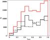 |
Fig. 1 Distribution of zpeak for galaxies in the CDFS (black line), COSMOS (dashed line) and in the overall sample (red line). |
2.2. Passive and star-forming galaxies
The rest frame colours of galaxies show a bimodal distribution that broadly reflects star-formation quenching: in general, “red” galaxies have had their star formation quenched, and “blue” galaxies are still forming stars (Blanton et al. 2003; Baldry et al. 2004). However, some star-forming galaxies exhibit red colours in spite of their young stars, due to the presence of dust.
The U−V vs. V−J colour−colour diagram allows for a simple separation of star-forming from passive galaxies: the U−V colour covers the Balmer break and is therefore a good measure of relatively unobscured recent star formation, while the V−J colour allows empirical separation of red passively evolving galaxies from red, dusty star-forming galaxies, since dust-free quiescent galaxies are relatively blue in V−J (e.g. Labbé et al. 2005; Williams et al. 2009; Brammer et al. 2009).
As in Muzzin et al. (2013b), we obtained rest frame U−V and V−J colours from the EAZY code, which measures the rest-frame fluxes from the best-fitting SED template (Brammer et al. 2008). The values of interpolated rest-frame colours primarily depends on the galaxy redshift and may be subject to systematic, redshift dependent offsets. Moreover, these offsets may be different depending on the SED templates (e.g. for quiescent and star-forming galaxies). Therefore, we verified that the distribution on the U−V vs. V−J colour−colour diagram for galaxies in the CDFS sample is very similar to that in the COSMOS sample, for which the estimate of photometric redshift is more accurate (Fig. 2).
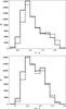 |
Fig. 2 Distribution of U−V (top panel) and V−J (bottom panel) rest frame colours for the CDFS (solid line) and the COSMOS (dashed line) galaxy samples. |
The rest frame U−V vs. V−J colour−colour diagram for galaxies in COSMOS, shown in Fig. 3 of Muzzin et al. (2013a), and in CDFS, shown here in Fig. 3, clearly display an extended sequence of star-forming galaxies (from the lower-left to the upper-right region) and a localised clump of passive galaxies in the upper region of the figure. Following Williams et al. (2009) and Muzzin et al. (2013a) we adopted the following criteria to select passive galaxies:
 (1)The conditions U−V> 1.3,V−J< 1.5 are applied to prevent contamination from unobscured and dusty star-forming galaxies, respectively. We found that the fraction of passive galaxies (approx. 12% and 18% in CDFS and COSMOS, respectively) and their distribution as a function of redshift are very similar in the two fields.
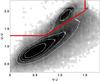 |
Fig. 3 Rest frame U−V vs. V−J colour−colour diagram for the CDFS galaxy sample. The solid red line separates passive from star-forming galaxies (Eq. (1)). |
2.3. Stellar masses, ages, SFR and sSFR
The wealth of photometric information for our samples allows us to apply the SED fitting technique to estimate the stellar mass and SFH for each galaxy of COSMOS and CDFS samples. We performed this fitting using the FITTING AND ASSESSMENT OF SYNTHETIC TEMPLATES (FAST)5 code (Kriek et al. 2009). To construct the set of template SEDs, we adopted: (i) the Bruzual & Charlot (2003) stellar population synthesis (SPS) model library; (ii) a Salpeter IMF; (iii) solar metallicity; (iv) an exponentially declining SFH (ψ(t) ∝ exp(−t/τ) where t is the time since the onset of the star formation and τ is the e-folding star formation timescale, ranging from 107 to 1010 Gyr and (v) the Calzetti et al. (2000) dust attenuation law. For all galaxies we restricted t to be less than the age of the Universe at the redshift of the galaxy and allowed for a visual attenuation in the range 0−4 mag. Redshifts were fixed to the values derived by EAZY.
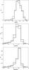 |
Fig. 4 Distribution of stellar masses (top panel), SFR (middle panel) and sSFR (bottom panel) estimated with FAST for the CDFS (solid line) and the COSMOS (dashed line) galaxy sample. |
In general, stellar masses estimated via the SED fitting technique are relatively well-constrained, however FAST does not account for the gas re-cycling and the return fraction, which is the fraction of mass of gas processed by stars and returned to the interstellar medium during their evolution. Therefore FAST overestimates the actual stellar mass by a fraction which amounts to 30% in an old stellar population for a Salpeter IMF (see e.g. Greggio & Renzini 2011). In Fig. 4 (top panel) we show the distribution of stellar masses for both COSMOS and CDFS samples. The COSMOS sample appears to include a larger fraction of low mass galaxies, compared to the CDFS sample.
The SFRs are more uncertain when they are derived solely from optical-NIR photometry and assumed to decline exponentially. The lack of FUV and MIR data that probe unobscured and obscured star formation, respectively, has an important effect on the estimate of SFR for galaxies experiencing a recent star formation burst. It is possible to analyse this effect by comparing the galaxy mass and SFR distribution for the COSMOS and the CDFS samples, since the photometry for galaxies in COSMOS field ranges from FUV to MIR bands. This comparison is shown in Fig. 4 (middle panel) where we notice that the SFR of the COSMOS galaxies is found to be systematically lower than that of the CDFS galaxies. Interestingly, the distribution of the sSFR, that is, the ratio between the current SFR and the galaxy mass, is the same for the two samples, even though the distributions in mass and SFR are slightly different (Fig. 4 bottom panel). The sSFR is less sensitive to the choice of IMF and input SPS models since the total SFR and mass both exhibit a similar dependence on these parameters (Williams et al. 2010).
SED fitting also leads to unrealistically low ages when applied to actively star-forming galaxies since the SED of such galaxies, at all wavelengths, is dominated by their youngest stellar populations, which outshine the older stellar populations that may inhabit these galaxies (Maraston et al. 2010). Thus, the SED of such galaxies conveys little information about the beginning of star formation, or, more specifically, on the age of their oldest stellar populations.
It is instructive to verify whether the separation of star-forming and quiescent galaxies on the U−V vs. V−J colour−colour space is well-correlated with separation using SED fitting-determined sSFRs (e.g. Williams et al. 2010). Figure 5 shows that blue star-forming galaxies exhibit higher sSFR with respect to passive red galaxies, suggesting that the separation of star-forming and passive galaxies based on colours is consistent with separation based on SED fitting. The star-forming galaxies also show lower masses and higher SFRs than the passive galaxies.
In the following we will estimate SN rates in star-forming and passive galaxies exploiting both methods to distinguish between the two classes.
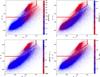 |
Fig. 5 Rest-frame U−V vs. V−J colour−colour plot for galaxies in the overall sample, colour-coded by stellar mass (top left), SFR (top right) and sSFR (bottom left), as derived from the SED fitting. In the bottom right panel the colour encoding reflects the rest frame de-reddened U−J colour. |
2.4. Intrinsic, dust-corrected colours
Historically, SN rates have been estimated as a function of U−V and B−K colours adopted as a proxy of the galaxy mean age (Cappellaro et al. 1999; Mannucci et al. 2005; Li et al. 2011). To compare the dependence of SN rates on the B−K colour in the local Universe and in the redshift range monitored by SUDARE, we estimated this rest-frame colour for the galaxies in our sample with EAZY. To correct the colour excess we exploited the extinction coefficients provided by FAST for each galaxy assuming the Calzetti et al. (2000) dust attenuation law. The distribution of rest-frame de-reddened B−K colour for the SUDARE and the local Universe galaxy samples is shown in Fig. 6. Galaxies in the SUDARE sample appear systematically bluer than those in the local sample in B−K colour. This is not unexpected, since local galaxies are, on average, older and characterised by a lower current SFR. Furthermore, our intrinsic colours have been estimated adopting the Calzetti et al. (2000) dust attenuation law which, having been calibrated on starburst galaxies, could overcorrect the extinction for galaxies with low star-formation activity. In the local Universe the intrinsic colours have been estimated and corrected for reddening using different methods.
In our analysis we also considered the intrinsic U−J colour an SFH tracer for our galaxies (see Sect. 9.1.2). This wavelength combination well-describes the contrast between the mass in young and old component. Moreover, the star-forming galaxies, identified as such as on the U−V vs. V−J colour−colour diagram, have rest frame de-reddened U−J colour bluer than the passive galaxies, as shown in Fig. 5. The distribution of the U−J colours of galaxies in the CDFS and in the COSMOS samples, shown in Fig. 7, is quite consistent.
3. SN sample
During the first two years of our programme we discovered 117 SNe, of which 57% are Type Ia, 19% Type II, 9% Type IIn and 15% Type Ib/c SNe. A detailed description of the process of the SN search, the criteria and algorithm for SN typing and characteristics of the SN sample (coordinates, type, redshift, discovery epoch, best fit template and reddening) can be found in Paper I.
The identification of the host galaxy for each SN in our sample has been obtained by measuring the separation of the SN from each candidate host galaxy in terms of an elliptical radius (R) defined by SExtractor via the equation:  (2)where xSN, ySN and xc, yc are the coordinates of the SN position and of the galaxy centre, respectively. We assumed that the isophotal limit of a given galaxy corresponds to R = 3. The identification of the correct host galaxy, the nearest in terms of R, has been verified through visual inspection and verification of the consistency of the host galaxy photometric redshift with the estimate of SN redshift from the photometric classification (see Paper I).
The host galaxies of 19 SNe were not detected in the Ks stacks, the host galaxies of 4 SNe were fainter than our selection limit (Ks = 23.5 mag), the hosts of 13 SNe had a poorly determined redshift (Qz > 1) and the hosts of 4 SNe had an unreasonable value for the SFR parameter (log(SFR) < −99). These 40 events have been discarded for the computation on the SN rates, since their hosts did not meet our selection criteria. This reduced the SN sample to 13 CC SNe in the redshift range 0.15 < z < 0.35 and 36 SNe Ia in the redshift range 0.15 < z < 0.75. We point out that the same criteria that lead to the exclusion of the 40 events mentioned above are also used to cull the whole galaxy sample, leading to a corresponding cull of galaxies in which no SN is detected. A fraction of SN candidates (10%) has an uncertain photometric classification, either because the light curve was not well sampled, or was affected by large photometric errors. These SNe have been classified and have been weighted by a factor of 0.5 in the rate calculation. The volumetric rates presented in Paper I are based on a larger number of events (26 CC SNe and 53 SNe Ia), since we selected all the SNe exploded within a given volume (0.15 < z < 0.35 and 0.15 < z < 0.75 for CC and Ia SNe, respectively) without any constraint on the host galaxies.
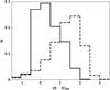 |
Fig. 6 Distribution of the B−K colour for galaxies in the local Universe (dashed line) monitored by the LOSS survey (Li et al. 2011), and for galaxies in the SUDARE sample (solid line). We converted colours in Li et al. (2011) from the Vega to the AB magnitude system. |
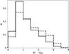 |
Fig. 7 The rest frame U−J colour in AB mag for the CDFS (solid line) and the COSMOS (dashed line) galaxy samples. |
4. SN rate
Since the probability of detecting a SN in one individual galaxy is low, it is customary to add the data relative to galaxies which are thought to share similar SFHs in order to constrain the trend of the SN rate with the parent stellar population on robust grounds. The binning of galaxies can be performed in different ways; for example, star-forming vs. passive galaxies, or, in general, according to their intrinsic (rest frame and de-reddened) colour. The total SN rate of the bin reflects the total SFH of the group, that is, the mass and the age distribution sampled in the bin.
4.1. SN rate and SFH
The SN rate in a given galaxy can be expressed as:
 (3)where t is the time elapsed since the beginning of star formation in the considered galaxy, ψ the SFR, kα(t−τ) is the number of stars per unit mass of the stellar generation born at epoch (t−τ), ASN(t−τ) is the number fraction of stars from this stellar generation that end up as SN, fSN is the delay time distribution (DTD) and τmin and τmax are the minimum and maximum possible delay times, respectively. The factor kα is given by:
  (4)where φ is the IMF and ml−mu is the mass range of the IMF. The factor ASN can be expressed as
  (5)where PSN is the probability that a star with suitable mass (mSN,u−mSN,l) actually becomes a SN. This probability depends on the SN progenitor models and on stellar evolution assumptions. The factors kα and ASN can vary with galaxy evolution, for example due to the effects of higher metallicities and/or the possible evolution of IMF. In the following we assume that kα, ASN and the IMF do not vary with time:
  (6)We also consider the DTD normalised to 1 over the total range of the delay times:
 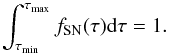 (7)If we assume that all stars with suitable mass (mCC,u−mCC,l) become CC SNe with a negligible delay time due to their short life time (3−20 Myr), and that the SFR has remained constant over this timescale, we consider that the rate of CC SNe is simply proportional to the current SFR, through a factor which is the number of CC progenitors per unit mass of the parent stellar population:
 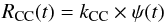 (8)with:
 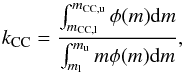 (9)where φ is the IMF and ml−mu is the mass range of the IMF. On the other hand, the time elapsed between the birth of SNe Ia progenitors and their explosions ranges from ~30 Myr to several billion years and controls the production rate of SNe Ia. For SNe Ia the observed rate includes progenitors born all along the past SFH:
 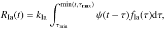 (10)where kIa = kα × AIa, the productivity of SNe Ia, is the number of type Ia SNe produced per unit mass of the parent stellar population:
 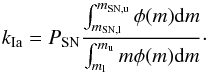 (11)
(11)
Both the productivity ( kIa) and the DTD ( fIa) of SNe Ia are sensitive to the model for their progenitors and depend on many parameters including the distribution of binary separations and of mass ratios and the outcome of the mass exchange phases, and of the final accretion on top of the WD.
In the literature one finds various approaches to measuring the SN rates, which use different proxies for the galaxy SFH. For example the SN rates have been measured in galaxies of different Hubble types (e.g. van den Bergh 1990; Ruiz-Lapuente et al. 1995), or U−V and B−K colours (e.g. Cappellaro et al. 1999; Mannucci et al. 2005; Li et al. 2011). In this paper we measure the SN rates as a function of B−K colour, in passive and star-forming galaxies identified as such on U−V vs. V−J colour−colour diagram and as a function of the sSFR estimated through the SED fitting technique.
4.2. Computing the SN rate
Three basic ingredients are required to estimate the SN rate in a galaxy sample: the number and type of SNe discovered, the time of effective surveillance of the sample (control time) in order to relate the detection frequency to the intrinsic SN rate and a physical parameter to normalise the rate.
The control time (CT) is defined as the time interval during which a SN occurring in a given galaxy can be detected in the search (Zwicky 1942). The CT of each individual observation depends on SN light curve, distance, reddening and efficiency of SN detection for that observation. The total CT is computed by properly summing the contribution of individual observations. The calculation of the CT is illustrated in detail in Paper I (Sect. 7.1)
In the literature, different normalisation factors, proportional to the content of stars that would eventually explode as SNe, have been adopted to compute the SN rate, such as the B-band luminosity (e.g. Cappellaro et al. 1999), H-band luminosity (e.g. van den Bergh 1990), the K-band luminosity (e.g. della Valle & Livio 1994; Mannucci et al. 2005; Li et al. 2011), the far-infrared luminosity (e.g. van den Bergh & Tammann 1991; Mannucci et al. 2003), the stellar mass derived from the K-band luminosity and the B−K colour (e.g. Mannucci et al. 2005; Li et al. 2011). In this paper we normalise the SN rates to the galaxy stellar mass, with the latter derived from the SED fitting, as in Sullivan et al. (2006) and Smith et al. (2012). The SN rate per unit mass is then computed as: 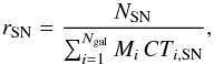 (12)where NSN is the total number of SNe of a given type, Ngal is the total number of galaxies and Mi, CTi,SN are the stellar mass and the control time of the ith galaxy, respectively. Galaxy masses in the literature are often referred to a Kroupa (2001) IMF. To compare our results with those of other authors we need to convert the rates per unit mass, SFRs and galaxy masses, to our IMF of choice, that is a Salpeter IMF between 0.1 and 100 M⊙. We do this by multiplying the masses obtained with a Kroupa (or equivalent) IMF by a factor of 1.36. This factor is the ratio between the total mass of SPSs and the same mass in stars heavier than 0.5 M⊙, yet with a different content of low mass stars, as the two IMFs require.
5. SN rates as a function of intrinsic colours
Mannucci et al. (2005) analysing the local sample of Cappellaro et al. (1999) demonstrated that the SN Ia rates per unit K band luminosity and per unit stellar mass have a very strong dependence on the galaxy Hubble type and B−K colour: blue galaxies exhibit an SN Ia rate larger than that of red galaxies by a factor of approximately 30 and confirm the earlier suggestions that a significant fraction of SNe Ia in late spirals/irregulars originates in a relatively young stellar component. The evidence that blue galaxies are more efficient in producing SN Ia events was interpreted by Oemler & Tinsley (1979) and Greggio & Renzini (1983) as being due to a DTD being more populated at short delay times (<1 Gyr). A similar SN Ia rate dependence on host galaxy colours was found by Li et al. (2011) for the LOSS sample that suggested an increase in SN Ia rate from red to blue galaxies by a factor of 6.5. For CC SNe the dependence of the rate on galaxy colours is more enhanced, as already noted by Cappellaro et al. (1999) and confirmed by Mannucci et al. (2005) and Li et al. (2011). The rate of the CC SNe in the early type galaxies is close to zero, it is small in the reddest galaxies, and in general becomes progressively higher in bluer galaxies.
Our measurements of both Type Ia and CC SN rates as a function of B−K are shown in Fig. 8 together with measurements in the local Universe. The SN Ia rate as a function of B−K colour from SUDARE is in good agreement with local measurements, following the same trend. The measurements of the CC SN rate from SUDARE are lower than the local ones in most colour bins, although consistent within the uncertainties. Our results suggest that there is no evolution with cosmic time of the dependence on galaxy colours for both SN CC and Ia rates.
 |
Fig. 8 SN rates as a function of B−K galaxy colour for SNe Ia (top panel) and CC SNe (bottom panel). For comparison we report the same measurements obtained in the local Universe by Mannucci et al. (2005) and by Li et al. (2011). The mass estimates for the galaxies by Mannucci et al. (2005) and Li et al. (2011) have been converted to a Salpeter IMF and B−K colours are all in AB mag. |
6. SN rates in passive and star-forming galaxies
The association between a colour sequence and a sequence in the SFR is not straightforward since the colours trace the global SFH in a galaxy, while the SFR refers to only the more recent past. The assumption of analytical expressions for the SFH in the SED fitting enforces a relation between the global colours and the recent SFR which may be inappropriate for the system. Moreover, the dust content and the presence of recent mergers can make the relations between SFR and the galaxy colours extremely complex. In Sect. 2.3 we showed that separation of star-forming and quiescent galaxies in U−V, V−J colour−colour space is reliable, thus to analyse the dependence of SN rates on SFR we split our host galaxy sample into passive and star-forming sub-samples following the prescription by Williams et al. (2009, Fig. 3). Our results are reported in Table 1 and show that the Type Ia SN rate is approximately a factor of five higher in the star-forming sample than in the passive sample. This supports the notion of a DTD declining with increasing delay time. There are not CC SNe discovered in the passive galaxies and we can measure only an upper limit for their rate. This is expected given the short lifetimes of CC SN progenitors which imply that the events die out soon after the end of the star formation activity. Furthermore, in star-forming galaxies we found a CC SN rate a factor two higher than the SN Ia rate.
SN rate per unit mass [10-3 SNe yr-1 10-10M⊙] in passive and star-forming galaxies, identified as such on the U−V, V−J diagram.
 |
Fig. 9 SN rates in SNuM vs. sSFR for Type Ia (left panel) and CC SNe (right panel) in three different groups of galaxies based on their sSFR: the first group of passive galaxies with a zero mean SFR; the second group of galaxies with −12.0 < log (sSFR) < −9.5; third group of galaxies with log (sSFR) > −9.5. In both panels the circles are from SUDARE, the triangles from Mannucci et al. (2005), the squares from Sullivan et al. (2006), the pentagons are from Smith et al. (2012) and the diamonds from Graur et al. (2015). The literature values have been corrected to a Salpeter IMF. |
SN rate per unit mass [10-3 SNe yr-1 10-10M⊙] in different bins of sSFR and galaxy mass as measured by FAST.
 |
Fig. 10 SN rates per unit stellar mass [10-3 SNe yr-1 10-10M⊙] as a function of the mass of the parent galaxy in the star-forming subsample for Type Ia (left panel) and CC SNe (right panel). In both panels the circles are from SUDARE, the triangles from Mannucci et al. (2005), the squares from Sullivan et al. (2006), the pentagons from Smith et al. (2012) and the diamonds from Graur et al. (2015). SN rates and masses have been rescaled to a Salpeter IMF. |
7. SN rates as a function of sSFR
The sSFR is a proxy for the SFH and the evolutionary stage of the galaxy. In particular the inverse of the sSFR defines a timescale for the formation of the stellar population of a galaxy. To compare our results to previous works we adopt the same criteria to separate passive and star-forming galaxies as in Sullivan et al. (2006), defining three galaxy groups based on the nature of star formation (see Fig. 9 figure legend). We stress that the condition log (sSFR) > −9.5 as division between highly and moderately star-forming is arbitrary.
Our results, illustrated in Table 2 and in Fig. 9, confirm the increase in the rate per unit stellar mass with increasing galaxy sSFR with approximately the same trend in the local Universe and at intermediate redshift. The enhancement of both SN Ia and CC SN rate from star-forming to starburst galaxies is steeper for CC SNe: we found an increase of approximately a factor of 5 for Type Ia and of 15 for CC SNe.
Figure 9 shows that the results from previous surveys yield a consistent increase of the SN Ia rate with increasing sSFR, with no evident dependence on redshift within the uncertainties. The difference between the SN Ia rate in passive galaxies and starburst galaxies is approximately a factor of 13 for our measurements, very close to estimates by Sullivan et al. (2006) in an almost identical range of redshift. A similar trend between the SN Ia rate per unit mass and the sSFR is reported by Graur et al. (2015) in the redshift range 0.04 <z< 0.2, while Smith et al. (2012) found a steeper increase from star-forming to starburst galaxies in the same range of redshift (0.05 <z< 0.25). We should mention that in the works of Sullivan et al. (2006) and Smith et al. (2012) the galaxy masses were determined via SED fitting to PEGASE 2.2 models and that the sSFR is measured as the ratio between the mean SFR over the last 0.5 Gyr and the current stellar mass of the galaxy. In the local Universe, Mannucci et al. (2005) adopted a galaxy classification based on the Hubble type and Sullivan et al. (2006) converted it to a sSFR classification, scaling rates in E/S0 to match their rate in passive galaxies.
The trend of SN Ia rate with the sSFR can be readily interpreted as shown in Greggio (2010, Fig. 12), and reflects the fact that the higher the SFR over the past 0.5 Gyr the higher the SN Ia rate. The similar scaling of the SN Ia rate with sSFR found at the different redshifts supports the notion that the ability of the stellar populations to produce SN Ia events does not vary with cosmic time.
The dependence of the CC SN rate per unit mass on the sSFR is expected to be linear since the CC SN rate is proportional to the recent SFR and the trend from SUDARE data is very similar to that observed in the local Universe (Mannucci et al. 2005) and in the redshift range 0.04 <z< 0.2 (Graur et al. 2015).
8. SN rates as a function of galaxy mass
In the recent literature several papers suggest that the rate of both SNe Ia and CC per unit stellar mass is proportional to the mass of the parent galaxy (Sullivan et al. 2006; Li et al. 2011; Graur et al. 2015), but with some controversy regarding the trend in passive and star-forming galaxies. Smith et al. (2012) suggest that the different results may be related to the different redshift ranges targeted in the various surveys.
The rate of CC SNe per unit mass is proportional to the sSFR and, since the latter is found to be lower in massive star-forming galaxies with respect to less massive ones (e.g. Schiminovich et al. 2007), it is expected that the CC SN rate per unit mass decreases for an increasing mass of the parent galaxy. The case for the rate of SN Ia is different. The SN Ia rate per unit mass of formed stars can be expressed as (see Eq. (10)): 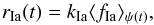 (13)where ⟨ fIa ⟩ is the average of the DTD weighted by the SFH over the whole galaxy lifetime. We point out that in Eq. (13) the rate is normalised to the integral of the SFR over the total galaxy lifetime, which is greater than the current mass in stars because of the mass return from stellar populations. From Eq. (13), a dependence of rIa on the mass of the parent galaxy may reflect a trend of either the SN Ia productivity (kIa), the shape of the DTD (fIa), or the SFH. Since the latter is known to be more populated at old ages in more massive galaxies (i.e. the downsizing phenomenon, e.g. Thomas et al. 2005), it is expected that the SN Ia rate per unit stellar mass is smaller in the more massive galaxies because these are older, and at long delay times the DTD is less populated than at short delays (Kistler et al. 2013). Figure 10 and Table 2 show the results of our survey for the star-forming galaxy sample, which are similar to those in the literature for both CC and Type Ia SNe. We find a trend of the SN Ia rate per unit stellar mass with the mass of the parent galaxy along the same slope as in Li et al. (2011). However, we note that our measurement in galaxies with low mass (log (M) < 9) seems to suggest a steeper trend with respect to that from the measurements by Sullivan et al. (2006) and by Smith et al. (2012). The trend for CC SN rate per unit stellar mass observed from SUDARE data is in good agreement with that from Graur et al. (2015) but not as steep as in Li et al. (2011). All in all, however, the relationship between the rate and galaxy mass for star-forming galaxies does not seem to vary with redshift, similar to what is found for the relationship between the colour and sSFR of the parent galaxy.
9. Comparison with models
We compare the observed SN rates with model predictions to derive constraints on the SN progenitors. The number of SNe (nSN) of a given type which we expect to detect in a galaxy of our sample can be expressed as: 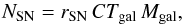 (14)where rSN is the SN rate per unit mass, the control time (CTgal) for the specific galaxy is computed as described in Sect. 4.2 and the galaxy mass (Mgal) is obtained from the SED fitting by FAST.
9.1. SNe Ia
In a galaxy that includes stars with ages up to AGE the SN Ia rate (rIa) per unit mass of formed stars can be written as: 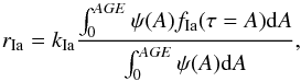 (15)where the variable A is the age of the stellar generations present in the galaxy, and ψ(A) is the SFH, expressed as the age distribution by mass in the galaxy. Thus, the SN Ia rate per unit mass is given by the productivity kIa, which we assume constant in time and the same in all galaxies, multiplied by the average DTD weighted by the SFH, or age distribution. The difference of the rate in different galaxies is totally ascribed to this second factor, and specifically to the age distribution, or SFH. The rate is the convolution between the age distribution and the DTD; therefore knowing the former, one may solve directly for the latter, as for example in Maoz et al. (2011) and in Childress et al. (2014). However, we think that the age distribution recovered from the SED fitting is not accurate enough to proceed along this line, and we prefer to test some physically motivated DTD models versus the observations.
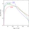 |
Fig. 11 Distributions of the delay times adopted in our modelling, selected from the family in Greggio (2005). SD (green solid): a single degenerate model which assumes Chandrasekhar mass explosions; SD1(green dashed): the same as SD up to a delay time of 0.5 Gyr, proportional to the inverse of the delay time onward; DDC (blue): a DD CLOSE model with parameters βa = −0.9,τn,x = 0.6; DDW (red): a DD WIDE model with parameters βa = 0,τn,x = 1. See Greggio (2005) for a description of the models. The DTD models are normalised to 1 over a range of delay times from 0 to 13 Gyr. |
As in Paper I, we select three DTD models from the realizations in Greggio (2005), showed in Fig. 11. Specifically, one SD model that assumes Chandrasekhar mass explosions, one very steep (DDC) and one very flat (DDW) DD model. The selected models correspond to a very different time evolution following a burst of star formation: 50% of the explosions occur within the first 0.45, 1.0, and 1.6 Gyr, for DDC, SD, and DDW models, respectively, while the late epoch decline scales as t-1.3 and t-0.8 for the DDC and DDW models, respectively. We add a fourth, DTD model (SD1) which is equal to the SD distribution for delay times shorter than 0.5 Gyr and falls off as t-1 at delay times longer than 0.5 Gyr. This DTD is similar to that adopted in Rodney et al. (2014). Compared to the SD model, the SD1 DTD maintains a relatively high rate in old stellar populations, with a late epoch decline. We perform the comparison of models with the observations in two ways: one relying on the SFH from FAST to predict the events in each galaxy and the other analysing the trend between the rate and the U−J colour of the parent galaxy, assumed to be a tracer of the age distribution.
9.1.1. Fit of the SNe Ia observed in the galaxies of the sample
We compute rIa/kIa adopting for fIa the DTD models in Fig. 11, and for the SFH the best fit parameters (AGE and τ) from FAST. For each galaxy of the sample we then derive the quantity nIa/kIa, and by summing them, we obtain the value of the productivity kIa required to reproduce the number of observed events.
We test the four DTD models mentioned above and two SFHs, namely an exponentially decreasing function ( ), and a delayed SFH (
 ), and for each combination we derive the SN Ia productivity (kIa). Table 3 also lists the expected number of SNe Ia in the passive and star-forming galaxy samples for the eight combinations of DTD model and SFH, having adopted the productivity normalised to the total number of events. In the SUDARE SN sample we count
  and
and  SN Ia in passive and star-forming galaxies, respectively. All errors are 1σ and were based on the confidence limits for small numbers according to Gehrels (1986). Comparing these figures with the expected events in Table 3, it seems that all combinations are similarly adequate, but that the DDW model is slightly disfavoured. The productivity is calculated to be approximately kIa = 0.001 M⊙-1, a value greater than that obtained in Paper I analysing the cosmic SN Ia rates as a function of redshift. In fact, assuming the cosmic SFH by Madau & Dickinson (2014), we found kIa = 7.5 × 10⁻⁴M⊙-1 for the SD and the DDW model and kIa = 8.5 × 10⁻⁴M⊙-1 for the DDC model. This discrepancy is not large, and we postpone the assessment of its significance until this survey is complete, when more robust statistics are available.
9.1.2. Rates as a function of galaxy colour
The method described in the previous section strongly relies on the SFH determined from the fit of the SED of each galaxy in the sample, and takes full advantage of the multi-band dataset. On the other hand, one can constrain the DTD through the analysis of the trend of the rate with the colour of the parent galaxy (e.g. Greggio 2005). In this approach, galaxies are stacked in colour bins, so that each bin samples a large stellar mass range, and the value of the rate benefits from a high statistical significance. At the same time, it is not necessary for the fitted SFH to be a precise representation for each galaxy; rather it is assumed that the average colour describes the global feature of the SFH of the bin, and the uncertainties on the individual SFHs are averaged out. We choose the U−J colour as representative of the global SFH: the U band is very sensitive to the young stellar populations, while the J band is a good tracer of the total mass.
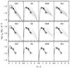 |
Fig. 12 Models of the SN Ia rate per unit mass as a function of the U−J colour of composite stellar populations obtained with different kinds of SFH and the four DTDs shown in Fig. 11. Along each line the parameter AGE of the composite stellar population varies from 0.05 (bluest point in U−J) to 13 Gyr (reddest point in U−J). In the top panels the assumed SFH is an exponentially declining law with e-folding times of (8,4.5,3.0,2.0,1.5,1.0,0.8,0.5,0.1) Gyr (left to right). In the central panels the assumed SFH is a delayed exponential model peaked at (20,10,7.5,5,3.5,2.0,1.0,0.5,0.1) Gyr (left to right). In the bottom panels the adopted SFH is a power law ψ(t) ∝ t− p with p ranging from 0 to 2.8: all these models describe the same locus, and do not account for populations redder than U−J ~ 2. The adopted values of the productivity are different for the different DTDs, and equal to |

 |
Fig. 13 Models of the SN Ia rate per unit mass as a function of the U−J colour for passive galaxies, as described by the evolution past a burst of star formation. Each curve refers to different durations of the bursts, namely (0.1,0.5,0.8,1,1.5,2,3,4.5,8) Gyr (top to bottom). Different panels show the results for different DTD models as labelled, and adopt the values for kIa as in Fig. 12, namely |

The lines in Fig. 12 show the trend of the SN Ia rate per unit mass with the colour of the parent galaxy as the parameter AGE increases, for different descriptions of the SFH, and the four selected DTD models. The productivity (kIa) for each DTD model has been chosen so as to reproduce the total number of events in the sample (see Table 3), while the colours have been computed with a SPS model based on Bruzual & Charlot (2003), with solar metallicity, as adopted for the SED fitting with FAST. In this way, the colours from the population synthesis agree with the rest frame de-reddened colours of galaxies in our sample, output of the EAZY and FAST codes. Open circles in Fig. 12 show the observed rates reported in Table 4 in star-forming galaxies, since the models SFH assume a currently active SFR. As in previous works (e.g. Mannucci et al. 2005; Greggio 2005) the SN Ia rate per unit mass decreases as the colour becomes redder, because the DTD models are more populated at short delay times, which implies a higher efficiency of SN Ia production in younger stellar populations. The slope of the trend depends on both the shape of the DTD and on the SFH, so that the diagnostic power of this kind of correlation is relatively poor, and all four DTD models appear equally compatible with the data.
SN Ia rate per unit mass [ ] as a function of U−J colour for galaxies in the redshift range 0.15 ≤ z< 0.75.
Considering now the rate in passive galaxies, we derive one important indication. Figure 13 shows the predicted trend of the SN Ia rate per unit mass as a function of U−J colour for a family of models meant to describe passive galaxies, which assume an initial burst of star formation, with a constant rate over a time interval Δt, which then drops to zero. The lines in the figure show the evolution of the rate and the colour of the produced stellar population from the end of the star formation episode onward, and different lines refer to different durations of this episode. The values adopted for kIa are the same as in Fig. 12. It is interesting to note that in passive galaxies after an initial stage in which the SN Ia rate stays constant as the color of the stellar population gets redder, all models converge to the same locus. This behaviour offers a diagnostic tool which does not seem to depend on the details of the SFH. The circle in Fig. 13 shows the rate and average colour of the passive galaxies. Only the DDC model meets the level of the rate and the colour of the passive galaxies simultaneously. Agreement between models and data could be found also for the other DTDs, but with a productivity of SN Ia higher than that appropriate for star-forming galaxies. Notice that our formalism does not allow for different values in kIa in different types of galaxies, while the trend of the rate with the properties of the parent galaxy should trace the different SFH, modulo the DTD. We also considered mixed models, with a contribution from both SD and DD channels, in the same fashion as Greggio (2010). Again we found that the combinations which include the DDC model provide a better fit to the star-forming and passive galaxies, while those with the DDW DTD tend to be too shallow to describe the rates in the passive and in the star-forming galaxies simultaneously.
9.1.3. Correlation of the rate with the galaxy mass
As pointed out previously, the SN Ia rate per unit mass in star-forming galaxies appears to decrease with increasing mass of the parent galaxy (see Fig. 10), an effect which could be ascribed to the downsizing phenomenon (see Sect. 8). But is downsizing present in our galaxy sample? To answer this question we binned our star-forming galaxies in four mass ranges, and within each range we computed the distribution of the galaxy mass-weighted average ages (⟨ Age ⟩), as given by:  (16)and calculated by adopting the best fit parameters from FAST to define ψ(A). Figure 14 shows the cumulative distribution of the average ages of the star-forming galaxies for the combined COSMOS and CDFS sample for the two options considered here to describe the SFH law.
The downsizing effect is indeed present in our sample, with the lower mass bin (blue line) hosting a larger fraction of galaxies with young average age. The solid horizontal line intercepts the distributions at the median average age of the four mass ranges, which gets older and older going from the least to the most massive bin, similar to what was found in Gallazzi et al. (2005). The average age distributions appear almost insensitive to the law adopted to describe the SFH. The dashed lines are drawn at the 30th and 70th percentiles in order to illustrate the width of the distributions of ⟨ Age ⟩ in the four mass bins.
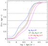 |
Fig. 14 Cumulative distributions of the average mass-weighted age of star-forming galaxies, in four bins of galaxy mass as labelled. The solid lines show the average ages relative to fits with the exponentially declining SFH; the dotted lines refer instead to fits which adopt the delayed SFH. The horizontal lines intercept the curves at the median (solid) average age and at the 30th and 70th percentiles (dashed). |
We model the effect of downsizing in our sample on the measured SN Ia rates by considering the correlation between the parameter ⟨ Age ⟩ and the rates in the family of models described in the previous section. Figure 15 shows such correlation for the exponentially declining SFH models in the case of the DDC description of the delay times distribution. Similar plots can be drawn for other DTD models. In general, the SN Ia rate per unit mass decreases as the average age of the parent galaxy increases, except for the systems with ⟨ Age ⟩ younger than ≃0.5 Gyr, for which it appears virtually constant. This characteristic reflects the wide peak of the DTD models at the short delay times. At average ages older than 0.5 Gyr, the rate declines with a slope sensitive to the e-folding timescale of the SFR, so that, at given ⟨ Age ⟩ the model rate spans a wide range, depending on the parameter τ. We find that the correlation between the SN Ia rate and the average age of the parent galaxy is very similar for the two SFHs considered here, while it turns out sensitive to the DTD, with the DDW delay time distribution providing a quite shallow correlation.
We now turn to consider the expected correlation between the SN Ia rate and the parent galaxy mass by combining the relation between ⟨ Age ⟩ and galaxy mass bin, and the correlation between ⟨ Age ⟩ and SN Ia rate. Rather then computing the expected rate for each galaxy in the sample, and examining the distribution of the results in the four mass bins, as in Graur et al. (2015), we compute the expected rate at some characteristic ⟨ Age ⟩ of the four mass bins, in particular at the intercepts of the horizontal lines with the four distributions in Fig. 14. Given the relatively poor statistics of SN Ia events collected to far, we aim to characterise the expected correlation and explore its variation with the DTD and the SFH. We will follow a more sophisticated approach once the survey has been completed. Figure 16 shows how the SN Ia rate is expected to vary in the four mass bins whose ⟨ Age ⟩ distributions are shown in Fig. 14.
Solid (red), and dashed (blue) lines connect the model rates at the median ⟨ Age ⟩ of the galaxies in the four mass bins, when adopting exponentially declining SFH models with e-folding times of 0.1 and 8 Gyr, respectively. At a given ⟨ Age ⟩, models with longer SFH timescales yield a higher rate, as depicted in Fig. 15. The four panels of Fig. 15 show the results for the four selected DTD models. Notice that for each DTD model the value of kIa comes from the fit described in Sect. 3.
The shaded areas illustrate the range of variation of the SN Ia rate model for the τ = 0.1 Gyr SFH models, corresponding to the 30th and 70th percentiles of the distribution of ⟨ Age ⟩ in the four bins of galaxy mass (see Fig. 14). Finally, the open circles are the observed rates.
The observed correlation is best reproduced by the combination of the DDC distribution of the delay times coupled to an exponentially decreasing SFH with short e-folding timescale. The models predict a relatively shallow correlation when the other three DTDs are considered, as well as when SFHs with long e-folding timescales are adopted. There is however ample room to accomodate either less steep DTDs and/or flatter SFHs if one considers the width of the distributions of the parameter ⟨ Age ⟩ within the four mass bins, as the shaded areas indicate. Similar considerations hold when the delayed SFH models are considered. As a cautionary note, we point out that these conclusions rely on the output SFHs from the FAST fit, and in particular on the distribution of the parameter ⟨ Age ⟩, or quantitive downsizing relation. In this respect we notice that the average ages of galaxies in Gallazzi et al. (2005) are systematically older than those found here by a factor which ranges from two to five, at the same average galaxy mass. This may be due to the different age tracers used in the two studies, and /or to the different galaxy samples. A thorough study of the SFH in the individual galaxies is required for a robust interpretation of the correlation between SN Ia rate and the mass of the parent galaxies.
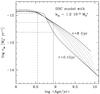 |
Fig. 15 Relation between the SN Ia rate model and the average age of the stars in the parent galaxy, for exponentially declining SFHs and a DDC model description of the DTD. The different solid lines are obtained for different values of the e-folding SF timescale, ranging from 0.1 Gyr (lowermost curve) to 8 Gyr (uppermost curve). Along each line the parameter AGE increases from 0.05 to 12.5 Gyr. The dashed and dotted lines are drawn at the median average ages, respectively, of the least and the most massive bin in Fig. 14. |
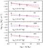 |
Fig. 16 SN Ia rate as a function of galaxy mass. Black circles are the observed rates in the four mass bins, reported in Table 2, while lines connect the theoretical rates at the median ⟨ Age ⟩ of the distributions in the four mass bins. Solid (red) and dashed (blue) lines refer to exponentially declining SFH models with τ = 0.1 and 8 Gyr, respectively. The shaded areas show the range covered when using the 30th or 70th percentiles of the ⟨ Age ⟩ distribution instead of the median ⟨ Age ⟩, for the exponentially declining SFH models with τ = 0.1 Gyr. |
9.2. CC SNe
For the CC SNe, we use Eq. (14) with the rate (rCC) given by Eq. (8). We adopt the SFR (ψ) from the FAST best fit and  , which corresponds to a progenitor mass range of 8 to 40 M⊙ for a Salpeter IMF. To estimate the CTgal for CC SNe we combined the CTs for each CC SN sub-type assuming the fraction of different sub-types reported in Paper I (56% II 40% Ibc and 4% IIn). We computed the expected number of CC SNe for each star-forming galaxy of the sample and the total number of expected CC SNe (nCC) by summing the contribution of each galaxy in the redshift range 0.15 <z< 0.35. The expected number of CC SNe is 21 in our galaxy sample while the observed number is
  (~60%). At face value, this discrepancy suggests a higher limit for the minimum progenitor mass, in the vicinity of ~10 M⊙. In Paper I comparing the volumetric CC SN rates as a function of redshift, we found agreement between the observed rates and the expectations from the cosmic SFH by Madau & Dickinson (2014) in combination with
  (see Sect. 8.1 in Paper I). The expected number of CC SNe in the sampled cosmic volume is 33, close to the number of discovered CC SNe, 26 events (~80%). We note that the selection criteria on the galaxy properties (see Sect. 3) have reduced the CC SN sample by a factor of two with respect to that exploited in Paper I. Therefore, we attribute part of the discrepancy between the expected and observed CC SNe to a fluctuation due to the relatively poor statistics, which is to be verified once the full data-set has been analysed. It is also interesting to compare the total volumetric SFRs in different redshift bins for the COSMOS galaxy sample to the volumetric SFRs by Madau & Dickinson (2014). Figure 17 shows the SFR density in different redshift bins estimated by summing the SFRs from the FAST code and the SFRs from the galaxy UV and NIR luminosity by Muzzin et al. (2013a) for the galaxy sample in the COSMOS field. In both cases we found higher values than those estimated assuming the SFH by Madau & Dickinson (2014). From this comparison we conclude that the cosmic SFH is not known with sufficient accuracy to allow us to pinpoint the value of kCC with an accuracy better than ~50%.
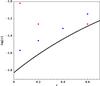 |
Fig. 17 SFR density as a function of redshift. The black line is the analytical function from Madau & Dickinson (2014). The red circles are measurements from SFRs in the COSMOS galaxy sample estimated by FAST SED fitting, while the blue points are measurements using UV and NIR luminosity by Muzzin et al. (2013a). |
10. Conclusions
The aim of the SUDARE survey is to constrain the SN progenitors analysing the dependence of the SN rate on the properties of the parent stellar population. The uncertainties in both SN rate and SFH measurements prevent an analysis based on individual galaxies, therefore we averaged over a population of galaxies with different ages and SFR following two different approaches.
In Paper I we measured the SN rates in a large volume as a function of the cosmic time, while in this work we measured the SN rates in a sample of galaxies as a function of the galaxy intrinsic colours or sSFR, both tracers of galaxy age.
The galaxy sample (approximately 130 000 galaxies) was obtained by selecting all galaxies the CDFS and COSMOS fields with (i) Ks band magnitude ≤23.5 mag; (ii) redshift within the range 0.15 ≤ z ≤ 0.75; and (iii) a reliable redshift estimate (Qz< 1). In order to estimate the photometric redshift and rest frame colours, we performed the SED fitting for each galaxy with the EAZY code. The galaxy mass, SFR and sSFR were estimated by the FAST code, with redshifts fixed to the values derived by EAZY, adopting the Bruzual & Charlot (2003) SPS model library, a Salpeter IMF, solar metallicity, an exponentially declining SFH and the Calzetti et al. (2000) dust attenuation law.
The separation of star-forming and quiescent galaxies was obtained by exploiting both the U−V vs. V−J colour−colour diagram, following the prescription by Williams et al. (2009), and the sSFR best fit values from FAST, adopting the same criteria as in Sullivan et al. (2006) (the passive galaxies with a zero mean SFR, the star-forming galaxies with −12.0 < log (sSFR) < −9.5, the star burst galaxies with log (sSFR) > −9.5).
In this galaxy sample we discovered 13 CC SNe in the redshift range 0.15 <z< 0.35 and 36 SNe Ia in the redshift range 0.15 <z< 0.75. The criteria and algorithm for SN search and photometric classification are illustrated in Paper I. The SN rates were measured with the method of the control time and normalised per unit stellar mass. Our principal findings are as follows.
-
1.
The trend of the SN rates as a function of the B−K colour of the parent galaxy from SUDARE data is consistent with that observed in the local Universe. Both CC and Type Ia SN rates become progressively higher for bluer galaxies but CC SNe have a steeper slope.
-
2.
The SN Ia rate per unit mass is approximately a factor of five higher in the star-forming- than in the passive galaxies, identified as such on the U−V vs. V−J colour−colour diagram. Only a lower limit for CC SN rate has been estimated in passive galaxies. This is expected given the short lifetimes of CC SN progenitors which imply that the CC SN rate is proportional to the recent SFR.
-
3.
The trend of the SN Ia rate as a function of the sSFR that we observed is very similar to previous results (Mannucci et al. 2005; Sullivan et al. 2006; Smith et al. 2012; Graur et al. 2015). Our results confirm that the higher the sSFR, the higher the SN Ia rate per unit mass suggesting a DTD declining with delay time. The fact that this trend is similar at the different redshifts suggests that the ability of the stellar populations to produce SN Ia events does not vary with cosmic time. The trend of the CC SN rate as a function of the sSFR is very similar to that observed in the local Universe (Mannucci et al. 2005) and in the redshift range 0.04 <z< 0.2 (Graur et al. 2015). This dependence is expected to be linear since the CC SN rate per unit mass is proportional to the sSFR.
-
4.
Our measurements of both CC and Type Ia SN rate per unit mass in the star-forming galaxy sample decrease for an increasing mass of the parent galaxy. The trend observed from SUDARE data is similar to that in Li et al. (2011) for both CC and Ia SNe. This trend is expected for CC SN rate per unit mass which is proportional to the sSFR, since the latter is found to be lower in massive star-forming galaxies than in less massive ones. The dependence of Type Ia SN rate on galaxy mass may reflect a trend of either the SN Ia productivity, the shape of the DTD or the SFH. Since the latter is known to be skewed towards old ages in more massive galaxies, it is expected that the SN Ia rate per unit mass is smaller in the more massive galaxies because these are older, and at long delay times the DTD is less populated than at short delays (<1 Gyr).
-
5.
The number of expected type Ia events for each galaxy has been determined by convolving the galaxy SFH from the FAST SED fitting with DTD models. The expected number of SNe Ia both in the passive and star-forming galaxy sample is in agreement with that observed for all DTD models considered, although the DDC model seems to be slightly favoured.
-
6.
We derive the SN Ia productivity by comparing the total number of SN Ia observed in our sample to the expected number of events obtained convolving the SFH in each galaxy with DTD models, and taking into account the appropriate control times. This normalisation made on the total sample, which includes passive and star-forming galaxies, yields similar values for kIa for the four DTD models considered, kIa = 1.2 × 10⁻³M⊙-1 for SD, kIa = 1.5 × 10⁻³M⊙-1 for DDW and kIa = 1.2 × 10⁻³M⊙-1 for DDC model. In Paper I we derived a complementary constraint on kIa by fitting the cosmic evolution of the SN Ia rate adopting the same DTD models as here, and the analytical formulation by Madau & Dickinson (2014) to describe the cosmic SFH. These kIa values are typically smaller that those derived here (
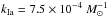 per SD and DDW model and kIa = 8.5 × 10⁻⁴M⊙-1 for DDC model). Given the different systematics affecting the two determinations we cannot assess with confidence the significance of this discrepancy.
 -
7.
The comparison between the observed and expected trend of the SN Ia rate with the intrinsic U−J colour of the parent galaxy in the star-forming sample is acceptable for all four DTD models. In the passive galaxies, only the DDC model meets the level of the rate and the colour of the passive galaxies simultaneously.
-
8.
We modelled the effect of downsizing in our galaxy sample on the SN Ia rate and found that the observed correlation between the SN Ia rate and the mass of the parent galaxy is best reproduced with a DDC model.
-
9.
The number of expected CC SN events for each star-forming galaxy has been estimated by assuming the SFR from the FAST SED fitting and a mass range of 8 to 40 M⊙ for CC SN progenitors, corresponding to
for a Salpeter IMF. The expected number of CC SNe is higher than that observed by a factor of approximately 40%. In Paper I the expected number of CC SN events was determined by assuming the SFH by Madau & Dickinson (2014) and the same value for the CC SN productivity and is higher than that observed by a factor of 20%. This discrepancy is due partly to a fluctuation caused by relatively poor statistics of CC SN events and partly to the difference between cosmic SFR and SFR best fit values from the FAST code.
We conclude from the observed correlations between the SN rates and properties of the parent galaxies that, according to the expectations of stellar evolution, the minimum mass for CC SN progenitors is between 8 and 10 M⊙ and that the DTD of SN Ia progenitors is skewed to short delay times (<1 Gyr). However, the uncertainties surrounding both CC and Type Ia SN rates are still too high to constrain the mass range of SN CC progenitors with sufficient accuracy and to discriminate between SD and DD progenitor scenarios.
 where Nfilt is the number of photometric measurements used in the fit, u99−l99 is the 99% confidence intervals and pΔz = 0.2 is the fractional probability that the redshift lies within ± 0.2 of the nominal value.
We denoted by zpeak the estimator which finds discrete peaks in the redshift probability function and returns the peak with the largest integrated probability.
Acknowledgments
We thank the referee for his/her useful comments and suggestions. This work is partially supported by the PRIN-INAF 2014 with the project “Transient Universe: unveiling new types of stellar explosions with PESSTO” (PI A. Pastorello). G.P. acknowledges support from the Proyecto Regular FONDECYT 1140352 and by Millennium Institute of Astrophysics (MAS) through grant IC120009 of the Programa Iniciativa Cientifica Milenio del Ministerio de Economia, Fomento y Turismo de Chile. M.V. acknowledges support from the Square Kilometre Array South Africa project, the South African National Research Foundation and Department of Science and Technology (DST/CON 0134/2014), the European Commission Research Executive Agency (FP7-SPACE-2013-1 GA 607254) and the Italian Ministry for Foreign Affairs and International Cooperation (PGR GA ZA14GR02).
References
- Baldry, I. K., Glazebrook, K., Brinkmann, J., et al. 2004, ApJ, 600, 681 [NASA ADS] [CrossRef] [Google Scholar]
- Bersten, M. C., Benvenuto, O. G., Nomoto, K., et al. 2012, ApJ, 757, 31 [NASA ADS] [CrossRef] [Google Scholar]
- Bersten, M. C., Benvenuto, O. G., Folatelli, G., et al. 2014, AJ, 148, 68 [NASA ADS] [CrossRef] [Google Scholar]
- Bianchi, S., & Schneider, R. 2007, MNRAS, 378, 973 [NASA ADS] [CrossRef] [Google Scholar]
- Blanton, M. R., Hogg, D. W., Bahcall, N. A., et al. 2003, ApJ, 594, 186 [NASA ADS] [CrossRef] [Google Scholar]
- Botticella, M. T., Cappellaro, E., Pignata, G., et al. 2013, The Messenger, 151, 29 [NASA ADS] [Google Scholar]
- Brammer, G. B., van Dokkum, P. G., & Coppi, P. 2008, ApJ, 686, 1503 [NASA ADS] [CrossRef] [Google Scholar]
- Brammer, G. B., Whitaker, K. E., van Dokkum, P. G., et al. 2009, ApJ, 706, L173 [NASA ADS] [CrossRef] [Google Scholar]
- Bruzual, G., & Charlot, S. 2003, MNRAS, 344, 1000 [NASA ADS] [CrossRef] [Google Scholar]
- Calzetti, D., Armus, L., Bohlin, R. C., et al. 2000, ApJ, 533, 682 [NASA ADS] [CrossRef] [Google Scholar]
- Cappellaro, E., Evans, R., & Turatto, M. 1999, A&A, 351, 459 [NASA ADS] [Google Scholar]
- Cappellaro, E., Botticella, M. T., Pignata, G., et al. 2015, A&A, 584, A62 [NASA ADS] [CrossRef] [EDP Sciences] [Google Scholar]
- Cao, Y., Kasliwal, M. M., Arcavi, I., et al. 2013, ApJ, 775, L7 [NASA ADS] [CrossRef] [Google Scholar]
- Ceverino, D., & Klypin, A. 2009, ApJ, 695, 292 [NASA ADS] [CrossRef] [Google Scholar]
- Chabrier, G. 2003, PASP, 115, 763 [NASA ADS] [CrossRef] [Google Scholar]
- Childress, M. J., Wolf, C., & Zahid, H. J. 2014, MNRAS, 445, 1898 [NASA ADS] [CrossRef] [Google Scholar]
- Dark Energy Survey Collaboration, Abbott, T., Abdalla, F. B., et al. 2016, MNRAS, 460, 1270 [NASA ADS] [CrossRef] [Google Scholar]
- della Valle, M., & Livio, M. 1994, ApJ, 423, L31 [NASA ADS] [CrossRef] [Google Scholar]
- Eldridge, J. J., Fraser, M., Smartt, S. J., Maund, J. R., & Crockett, R. M. 2013, MNRAS, 436, 774 [NASA ADS] [CrossRef] [Google Scholar]
- Eldridge, J. J., Fraser, M., Maund, J. R., & Smartt, S. J. 2015, MNRAS, 446, 2689 [NASA ADS] [CrossRef] [Google Scholar]
- Fremling, C., Sollerman, J., Taddia, F., et al. 2016, A&A, 593, A68 [NASA ADS] [CrossRef] [EDP Sciences] [Google Scholar]
- Fryer, C. L., Belczynski, K., Wiktorowicz, G., et al. 2012, ApJ, 749, 91 [NASA ADS] [CrossRef] [Google Scholar]
- Gallazzi, A., Charlot, S., Brinchmann, J., White, S. D. M., & Tremonti, C. A. 2005, MNRAS, 362, 41 [NASA ADS] [CrossRef] [Google Scholar]
- Gehrels, N. 1986, ApJ, 303, 336 [NASA ADS] [CrossRef] [Google Scholar]
- Graur, O., Bianco, F. B., & Modjaz, M. 2015, MNRAS, 450, 905 [NASA ADS] [CrossRef] [Google Scholar]
- Greggio, L. 2005, A&A, 441, 1055 [NASA ADS] [CrossRef] [EDP Sciences] [Google Scholar]
- Greggio, L. 2010, MNRAS, 406, 22 [NASA ADS] [CrossRef] [Google Scholar]
- Greggio, L., & Renzini, A. 1983, A&A, 118, 217 [NASA ADS] [Google Scholar]
- Greggio, L., & Renzini, A. 2011, Stellar Populations: a User Guide from Low to High Redshift (Wiley-VCH-Verlag) [Google Scholar]
- Greggio, L., Renzini, A., & Daddi, E. 2008, MNRAS, 388, 829 [NASA ADS] [CrossRef] [Google Scholar]
- Gunn, J. E., Carr, M., Rockosi, C., et al. 1998, AJ, 116, 3040 [NASA ADS] [CrossRef] [Google Scholar]
- Heger, A., Fryer, C. L., Woosley, S. E., Langer, N., & Hartmann, D. H. 2003, ApJ, 591, 288 [NASA ADS] [CrossRef] [Google Scholar]
- Iben, Jr., I., & Tutukov, A. V. 1984, ApJS, 54, 335 [NASA ADS] [CrossRef] [Google Scholar]
- Jarvis, M. J., Bonfield, D. G., Bruce, V. A., et al. 2013, MNRAS, 428, 1281 [NASA ADS] [CrossRef] [Google Scholar]
- Kistler, M. D., Stanek, K. Z., Kochanek, C. S., Prieto, J. L., & Thompson, T. A. 2013, ApJ, 770, 88 [NASA ADS] [CrossRef] [Google Scholar]
- Kriek, M., van Dokkum, P. G., Labbé, I., et al. 2009, ApJ, 700, 221 [NASA ADS] [CrossRef] [Google Scholar]
- Kroupa, P. 2001, MNRAS, 322, 231 [NASA ADS] [CrossRef] [Google Scholar]
- Labbé, I., Huang, J., Franx, M., et al. 2005, ApJ, 624, L81 [NASA ADS] [CrossRef] [Google Scholar]
- Li, W., Chornock, R., Leaman, J., et al. 2011, MNRAS, 412, 1473 [NASA ADS] [CrossRef] [Google Scholar]
- Lonsdale, C. J., Smith, H. E., Rowan-Robinson, M., et al. 2003, PASP, 115, 897 [NASA ADS] [CrossRef] [Google Scholar]
- Madau, P., & Dickinson, M. 2014, ARA&A, 52, 415 [NASA ADS] [CrossRef] [Google Scholar]
- Mannucci, F., Maiolino, R., Cresci, G., et al. 2003, A&A, 401, A519 [NASA ADS] [CrossRef] [EDP Sciences] [Google Scholar]
- Mannucci, F., Della Valle, M., Panagia, N., et al. 2005, A&A, 433, 807 [NASA ADS] [CrossRef] [EDP Sciences] [Google Scholar]
- Maoz, D., Mannucci, F., Li, W., et al. 2011, MNRAS, 412, 1508 [NASA ADS] [CrossRef] [Google Scholar]
- Maoz, D., Mannucci, F., & Brandt, T. D. 2012, MNRAS, 426, 3282 [NASA ADS] [CrossRef] [Google Scholar]
- Maoz, D., Mannucci, F., & Nelemans, G. 2014, ARA&A, 52, 107 [NASA ADS] [CrossRef] [Google Scholar]
- Maraston, C., Pforr, J., Renzini, A., et al. 2010, MNRAS, 407, 830 [NASA ADS] [CrossRef] [Google Scholar]
- Mauduit, J.-C., Lacy, M., Farrah, D., et al. 2012, AAS Meet. Abstr., 219, 446.19 [Google Scholar]
- Mobasher, B., Dahlen, T., Ferguson, H. C., et al. 2015, ApJ, 808, 101 [NASA ADS] [CrossRef] [Google Scholar]
- Muzzin, A., Marchesini, D., Stefanon, M., et al. 2013a, ApJ, 777, 18 [NASA ADS] [CrossRef] [Google Scholar]
- Muzzin, A., Marchesini, D., Stefanon, M., et al. 2013b, ApJS, 206, 8 [Google Scholar]
- Oemler, A., Jr., & Tinsley, B. M. 1979, AJ, 84, 985 [NASA ADS] [CrossRef] [Google Scholar]
- Perlmutter, S., Aldering, G., della Valle, M., et al. 1998, Nature, 391, 51 [CrossRef] [Google Scholar]
- Perlmutter, S., Aldering, G., Goldhaber, G., et al. 1999, ApJ, 517, 565 [NASA ADS] [CrossRef] [Google Scholar]
- Pforr, J., Maraston, C., & Tonini, C. 2012, MNRAS, 422, 3285 [NASA ADS] [CrossRef] [Google Scholar]
- Pforr, J., Maraston, C., & Tonini, C. 2013, MNRAS, 435, 1389 [NASA ADS] [CrossRef] [Google Scholar]
- Riess, A. G., Filippenko, A. V., Challis, P., et al. 1998, AJ, 116, 1009 [NASA ADS] [CrossRef] [Google Scholar]
- Rodney, S. A., Riess, A. G., Strolger, L.-G., et al. 2014, AJ, 148, 13 [NASA ADS] [CrossRef] [Google Scholar]
- Ruiz-Lapuente, P., Burkert, A., & Canal, R. 1995, ApJ, 447, L69 [NASA ADS] [CrossRef] [Google Scholar]
- Salpeter, E. E. 1955, ApJ, 121, 161 [Google Scholar]
- Salzano, V., Rodney, S. A., Sendra, I., et al. 2013, A&A, 557, A64 [NASA ADS] [CrossRef] [EDP Sciences] [Google Scholar]
- Schiminovich, D., Wyder, T. K., Martin, D. C., et al. 2007, ApJS, 173, 315 [NASA ADS] [CrossRef] [Google Scholar]
- Schmidt, B. P., Suntzeff, N. B., Phillips, M. M., et al. 1998, ApJ, 507, 46 [NASA ADS] [CrossRef] [Google Scholar]
- Smartt, S. J. 2009, ARA&A, 47, 63 [NASA ADS] [CrossRef] [Google Scholar]
- Smith, N., Li, W., Filippenko, A. V., & Chornock, R. 2011, MNRAS, 412, 1522 [NASA ADS] [CrossRef] [Google Scholar]
- Smith, M., Nichol, R. C., Dilday, B., et al. 2012, ApJ, 755, 61 [NASA ADS] [CrossRef] [Google Scholar]
- Sullivan, M., Le Borgne, D., Pritchet, C. J., et al. 2006, ApJ, 648, 868 [NASA ADS] [CrossRef] [Google Scholar]
- Sullivan, M., Guy, J., Conley, A., et al. 2011, ApJ, 737, 102 [NASA ADS] [CrossRef] [Google Scholar]
- Thomas, D., Maraston, C., Bender, R., & Mendes de Oliveira, C. 2005, ApJ, 621, 673 [NASA ADS] [CrossRef] [Google Scholar]
- Tutukov, A. V., & Yungelson, L. R. 1981, Nauchnye Informatsii, 49, 3 [NASA ADS] [Google Scholar]
- Vaccari, M. 2015, Proc. of Conf. The Many Facets of Extragalactic Radio Surveys: Towards New Scientific Challenges, 27 [Google Scholar]
- van den Bergh, S. 1990, PASP, 102, 1318 [NASA ADS] [CrossRef] [Google Scholar]
- van den Bergh, S., & Tammann, G. A. 1991, ARA&A, 29, 363 [NASA ADS] [CrossRef] [Google Scholar]
- Whelan, J., & Iben, Jr., I. 1973, ApJ, 186, 1007 [NASA ADS] [CrossRef] [Google Scholar]
- Williams, R. J., Quadri, R. F., Franx, M., van Dokkum, P., & Labbé, I. 2009, ApJ, 691, 1879 [NASA ADS] [CrossRef] [Google Scholar]
- Williams, R. J., Quadri, R. F., Franx, M., et al. 2010, ApJ, 713, 738 [NASA ADS] [CrossRef] [Google Scholar]
- Wittman, D. 2009, ApJ, 700, L174 [NASA ADS] [CrossRef] [Google Scholar]
- Woosley, S. E., & Bloom, J. S. 2006, ARA&A, 44, 507 [NASA ADS] [CrossRef] [Google Scholar]
- Zwicky, F. 1942, ApJ, 96, 28 [NASA ADS] [CrossRef] [Google Scholar]
Appendix A: CC SN subtypes
SN rate per unit mass [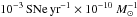 ] for different bin of sSFR.
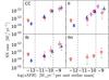 |
Fig. A.1 SN rates per unit stellar mass vs. sSFR for different CC SN types in three different groups of galaxies based on their sSFR: the first group of passive galaxies with a zero mean SFR, the second group of galaxies with −12.0 < log (sSFR) < −9.5 and the third group of galaxies with log (sSFR) > −9.5. The circles are from SUDARE, the triangles from Mannucci et al. (2005) and the pentagons from Graur et al. (2015). |
We estimated the rates for different CC SN sub-types (II, Ibc and IIn) as a function of both the sSFR and the stellar mass (Table A.1 and Fig. 9). Although our SN sample remains small, it is adequate enough to show a good match with the SN rates in the local Universe (Mannucci et al. 2005) and at intermediate redshift (Graur et al. 2015). Particularly, our measurement of the Type II SN rate in starburst galaxies is not significantly lower than the measurement from Graur et al. (2015) in the redshift range 0.1 < z < 0.4. The trend of the rate as a function of stellar mass for both Type II and Type Ib/c SNe is similar to that obtained from Li et al. (2011). A lack of statistics prevents us from confirming the suggestion by Li et al. (2011) that the Type Ib/c SN rates are deficient relative to the Type II rates in less-massive galaxies since we found very similar values for them.
Appendix B: Systematic errors
Rest frame colours, mass and sSFR, as determined from broad band photometry, suffer from various uncertainties related to incomplete coverage of photometric bands, errors in photometric redshifts, incorrect assumptions in SED fitting and the systematic interplay between these parameters.
Several studies have recently presented a comprehensive analysis of the accuracy of the galaxy properties estimated through SED fitting as a function of the various parameters (SFH, metallicity, age grid, IMF, reddening law, wavelength coverage and filter setup), both in passive- and star-forming galaxies and in a wide redshift range (Pforr et al. 2012, 2013; Mobasher et al. 2015). In the following we discuss the impact of systematics affecting galaxies samples on our results.
Photometric redshifts. We explored different methods in assessing the quality of photometric redshifts and discussed them in detail in Paper I. Here we only analyse the effects of choosing a redshift estimator different from zpeak6 on SED fitting. In this test we adopted zMC, which is drawn randomly from the redshift probability distribution and incorporates the redshift uncertainties (Wittman 2009). The comparison between the distributions of the photometric redshifts obtained by adopting alternatively zMC or zpeak is analysed in Paper I for both CDFS and COSMOS fields. We find that the distributions of mass, SFR and sSFR obtained with zMC and zpeak in input to FAST are very similar for both the CDFS and the COSMOS sample, as shown in Fig. B.1. The SN rates per unit stellar mass as a function of sSFR measured by adopting zMC in the SED fitting are reported in Table B.1. The errors due to photometric redshift uncertainty are negligible with respect to the statistical errors for both Type Ia and CC SN rate. We note that the errors estimated for CC SN rates are higher than those for SN Ia rates.
SFH.Pforr et al. (2012) after analysing the accuracy of galaxy properties as a function of the various parameters of the SED fitting found that the most important parameter in recovering stellar mass is the SFH, in agreement with Maraston et al. (2010). Mobasher et al. (2015) performed a similar study to quantify the differences between the stellar masses estimated using different SED templates and different fitting techniques. In agreement with previous studies, they found that the lack of knowledge of the correct SFH, combined with inherent degeneracy between age, dust and metallicity, are the main reasons for uncertainties in the stellar masses. We analysed the distribution of some galaxy properties obtained assuming a different SFH, and a delayed exponentially declining function (ψdel ∝ t × exp(−t/τ), where t is the time since the onset of SF and τ is a parameter, ranging from 108−1010 Gyr. The distributions of galaxy mass, SFR and sSFR for the two adopted SFH laws are shown in Fig. B.1 for the CDFS galaxy sample. We note that the distributions of galaxy masses are very similar, while the distributions of SFR and sSFR show more galaxies with higher SFR and sSFR for the delayed SFH assumption. The SN rate measurements obtained by assuming ψdel are reported in Table B.1. The errors due to the uncertainty in the SFH assumption are negligible with respect to statistical errors for both SN CC and Ia rates.
IMF. We also analysed the sensitivity of the SED fitting to the IMF choice. Recent studies showed that different choices on the IMF produce different estimates of stellar mass and age, especially for top-heavy IMFs. We checked how the parameters from our SED fitting vary when the template setups are compiled using Salpeter and Chabrier IMFs (Salpeter 1955; Chabrier 2003). We found that the sSFRs are very similar but that the masses and SFRs, obtained assuming a Chabrier (2003) IMF, are systematically lower by ~0.2 dex. This is expected since these two IMFs essentially differ for the mass fraction in stars more massive than 1 M⊙, which amounts to fhigh = 0.61 and 0.39 for Chabrier and Salpeter IMF, respectively. Since these stars contribute almost the total light of the stellar population, the mass to light ratio scales as 1 /fhigh. Therefore, at a given total luminosity, the Chabrier IMF yields a total mass which is a factor of ~1.6 lower than obtained with Salpeter IMF. When we adopt a Chabrier (2003) IMF, the SN rates become higher by a factor of two in the bins with higher sSFR. The errors estimated assuming a different IMF are larger than those in the previous cases.
SN rates per unit mass [ ] in different bins of sSFR obtained by adopting a different redshift estimator (zMC), a delayed exponentially declining SFH (SFHdel) and a different IMF (Chabrier) in the SED fitting.
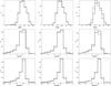 |
Fig. B.1 Top panel: the different distributions of stellar masses for galaxies in CDFS obtained from the SED fitting assuming, in the left panel, zpeak (black line) and zMC (dotted line), in the middle panel ψ ∝ exp(−t/τ (black line) and ψdel ∝ t × exp(−t/τ (dotted line), in the right panel a Salpeter (black line) and Chabrier (dotted line) IMF. Middle panel: the different distributions of SFRs for galaxies in CDFS obtained from the SED fitting assuming, in theleft panel, zpeak (black line) and zMC (dotted line), in the middle panel ψ ∝ exp(−t/τ (black line) and ψdel ∝ t × exp(−t/τ (dotted line), in the right panel a Salpeter (black line) and Chabrier (dotted line) IMF. Bottom panel: the different distributions of sSFR for galaxies in CDFS obtained from the SED fitting assuming, in the left panel, zpeak (black line) and zMC (dotted line), in the middle panel ψ ∝ exp(−t/τ (black line) and ψdel ∝ t × exp(−t/τ (dotted line), in the right panel a Salpeter (black line) and Chabrier (dotted line) IMF. |
All Tables
SN rate per unit mass [10-3 SNe yr-1 10-10M⊙] in passive and star-forming galaxies, identified as such on the U−V, V−J diagram.
SN rate per unit mass [10-3 SNe yr-1 10-10M⊙] in different bins of sSFR and galaxy mass as measured by FAST.
SN Ia rate per unit mass [] as a function of U−J colour for galaxies in the redshift range 0.15 ≤ z< 0.75.
SN rates per unit mass [] in different bins of sSFR obtained by adopting a different redshift estimator (zMC), a delayed exponentially declining SFH (SFHdel) and a different IMF (Chabrier) in the SED fitting.
All Figures
|
Fig. 1 Distribution of zpeak for galaxies in the CDFS (black line), COSMOS (dashed line) and in the overall sample (red line). |
| In the text | |
|
Fig. 2 Distribution of U−V (top panel) and V−J (bottom panel) rest frame colours for the CDFS (solid line) and the COSMOS (dashed line) galaxy samples. |
| In the text | |
|
Fig. 3 Rest frame U−V vs. V−J colour−colour diagram for the CDFS galaxy sample. The solid red line separates passive from star-forming galaxies (Eq. (1)). |
| In the text | |
|
Fig. 4 Distribution of stellar masses (top panel), SFR (middle panel) and sSFR (bottom panel) estimated with FAST for the CDFS (solid line) and the COSMOS (dashed line) galaxy sample. |
| In the text | |
|
Fig. 5 Rest-frame U−V vs. V−J colour−colour plot for galaxies in the overall sample, colour-coded by stellar mass (top left), SFR (top right) and sSFR (bottom left), as derived from the SED fitting. In the bottom right panel the colour encoding reflects the rest frame de-reddened U−J colour. |
| In the text | |
|
Fig. 6 Distribution of the B−K colour for galaxies in the local Universe (dashed line) monitored by the LOSS survey (Li et al. 2011), and for galaxies in the SUDARE sample (solid line). We converted colours in Li et al. (2011) from the Vega to the AB magnitude system. |
| In the text | |
|
Fig. 7 The rest frame U−J colour in AB mag for the CDFS (solid line) and the COSMOS (dashed line) galaxy samples. |
| In the text | |
|
Fig. 8 SN rates as a function of B−K galaxy colour for SNe Ia (top panel) and CC SNe (bottom panel). For comparison we report the same measurements obtained in the local Universe by Mannucci et al. (2005) and by Li et al. (2011). The mass estimates for the galaxies by Mannucci et al. (2005) and Li et al. (2011) have been converted to a Salpeter IMF and B−K colours are all in AB mag. |
| In the text | |
|
Fig. 9 SN rates in SNuM vs. sSFR for Type Ia (left panel) and CC SNe (right panel) in three different groups of galaxies based on their sSFR: the first group of passive galaxies with a zero mean SFR; the second group of galaxies with −12.0 < log (sSFR) < −9.5; third group of galaxies with log (sSFR) > −9.5. In both panels the circles are from SUDARE, the triangles from Mannucci et al. (2005), the squares from Sullivan et al. (2006), the pentagons are from Smith et al. (2012) and the diamonds from Graur et al. (2015). The literature values have been corrected to a Salpeter IMF. |
| In the text | |
|
Fig. 10 SN rates per unit stellar mass [10-3 SNe yr-1 10-10M⊙] as a function of the mass of the parent galaxy in the star-forming subsample for Type Ia (left panel) and CC SNe (right panel). In both panels the circles are from SUDARE, the triangles from Mannucci et al. (2005), the squares from Sullivan et al. (2006), the pentagons from Smith et al. (2012) and the diamonds from Graur et al. (2015). SN rates and masses have been rescaled to a Salpeter IMF. |
| In the text | |
|
Fig. 11 Distributions of the delay times adopted in our modelling, selected from the family in Greggio (2005). SD (green solid): a single degenerate model which assumes Chandrasekhar mass explosions; SD1(green dashed): the same as SD up to a delay time of 0.5 Gyr, proportional to the inverse of the delay time onward; DDC (blue): a DD CLOSE model with parameters βa = −0.9,τn,x = 0.6; DDW (red): a DD WIDE model with parameters βa = 0,τn,x = 1. See Greggio (2005) for a description of the models. The DTD models are normalised to 1 over a range of delay times from 0 to 13 Gyr. |
| In the text | |
|
Fig. 12 Models of the SN Ia rate per unit mass as a function of the U−J colour of composite stellar populations obtained with different kinds of SFH and the four DTDs shown in Fig. 11. Along each line the parameter AGE of the composite stellar population varies from 0.05 (bluest point in U−J) to 13 Gyr (reddest point in U−J). In the top panels the assumed SFH is an exponentially declining law with e-folding times of (8,4.5,3.0,2.0,1.5,1.0,0.8,0.5,0.1) Gyr (left to right). In the central panels the assumed SFH is a delayed exponential model peaked at (20,10,7.5,5,3.5,2.0,1.0,0.5,0.1) Gyr (left to right). In the bottom panels the adopted SFH is a power law ψ(t) ∝ t− p with p ranging from 0 to 2.8: all these models describe the same locus, and do not account for populations redder than U−J ~ 2. The adopted values of the productivity are different for the different DTDs, and equal to |
| In the text | |
|
Fig. 13 Models of the SN Ia rate per unit mass as a function of the U−J colour for passive galaxies, as described by the evolution past a burst of star formation. Each curve refers to different durations of the bursts, namely (0.1,0.5,0.8,1,1.5,2,3,4.5,8) Gyr (top to bottom). Different panels show the results for different DTD models as labelled, and adopt the values for kIa as in Fig. 12, namely |
| In the text | |
|
Fig. 14 Cumulative distributions of the average mass-weighted age of star-forming galaxies, in four bins of galaxy mass as labelled. The solid lines show the average ages relative to fits with the exponentially declining SFH; the dotted lines refer instead to fits which adopt the delayed SFH. The horizontal lines intercept the curves at the median (solid) average age and at the 30th and 70th percentiles (dashed). |
| In the text | |
|
Fig. 15 Relation between the SN Ia rate model and the average age of the stars in the parent galaxy, for exponentially declining SFHs and a DDC model description of the DTD. The different solid lines are obtained for different values of the e-folding SF timescale, ranging from 0.1 Gyr (lowermost curve) to 8 Gyr (uppermost curve). Along each line the parameter AGE increases from 0.05 to 12.5 Gyr. The dashed and dotted lines are drawn at the median average ages, respectively, of the least and the most massive bin in Fig. 14. |
| In the text | |
|
Fig. 16 SN Ia rate as a function of galaxy mass. Black circles are the observed rates in the four mass bins, reported in Table 2, while lines connect the theoretical rates at the median ⟨ Age ⟩ of the distributions in the four mass bins. Solid (red) and dashed (blue) lines refer to exponentially declining SFH models with τ = 0.1 and 8 Gyr, respectively. The shaded areas show the range covered when using the 30th or 70th percentiles of the ⟨ Age ⟩ distribution instead of the median ⟨ Age ⟩, for the exponentially declining SFH models with τ = 0.1 Gyr. |
| In the text | |
|
Fig. 17 SFR density as a function of redshift. The black line is the analytical function from Madau & Dickinson (2014). The red circles are measurements from SFRs in the COSMOS galaxy sample estimated by FAST SED fitting, while the blue points are measurements using UV and NIR luminosity by Muzzin et al. (2013a). |
| In the text | |
|
Fig. A.1 SN rates per unit stellar mass vs. sSFR for different CC SN types in three different groups of galaxies based on their sSFR: the first group of passive galaxies with a zero mean SFR, the second group of galaxies with −12.0 < log (sSFR) < −9.5 and the third group of galaxies with log (sSFR) > −9.5. The circles are from SUDARE, the triangles from Mannucci et al. (2005) and the pentagons from Graur et al. (2015). |
| In the text | |
|
Fig. B.1 Top panel: the different distributions of stellar masses for galaxies in CDFS obtained from the SED fitting assuming, in the left panel, zpeak (black line) and zMC (dotted line), in the middle panel ψ ∝ exp(−t/τ (black line) and ψdel ∝ t × exp(−t/τ (dotted line), in the right panel a Salpeter (black line) and Chabrier (dotted line) IMF. Middle panel: the different distributions of SFRs for galaxies in CDFS obtained from the SED fitting assuming, in theleft panel, zpeak (black line) and zMC (dotted line), in the middle panel ψ ∝ exp(−t/τ (black line) and ψdel ∝ t × exp(−t/τ (dotted line), in the right panel a Salpeter (black line) and Chabrier (dotted line) IMF. Bottom panel: the different distributions of sSFR for galaxies in CDFS obtained from the SED fitting assuming, in the left panel, zpeak (black line) and zMC (dotted line), in the middle panel ψ ∝ exp(−t/τ (black line) and ψdel ∝ t × exp(−t/τ (dotted line), in the right panel a Salpeter (black line) and Chabrier (dotted line) IMF. |
| In the text | |
Current usage metrics show cumulative count of Article Views (full-text article views including HTML views, PDF and ePub downloads, according to the available data) and Abstracts Views on Vision4Press platform.
Data correspond to usage on the plateform after 2015. The current usage metrics is available 48-96 hours after online publication and is updated daily on week days.
Initial download of the metrics may take a while.