| Issue |
A&A
Volume 598, February 2017
|
|
|---|---|---|
| Article Number | A26 | |
| Number of page(s) | 13 | |
| Section | Planets and planetary systems | |
| DOI | https://doi.org/10.1051/0004-6361/201628985 | |
| Published online | 26 January 2017 | |
HADES RV Programme with HARPS-N at TNG
II. Data treatment and simulations⋆
1 Institut de Ciències de l’Espai (CSIC-IEEC), Campus UAB, Carrer de Can Magrans s/n, 08193 Cerdanyola del Vallès, Spain
e-mail: This email address is being protected from spambots. You need JavaScript enabled to view it.
2 INAF–Osservatorio Astronomico di Palermo, Piazza del Parlamento 1, 90134 Palermo, Italy
3 INAF–Osservatorio Astrofisico di Torino, via Osservatorio 20, 10025 Pino Torinese, Italy
4 Instituto de Astrofísica de Canarias (IAC), 38205 La Laguna, Tenerife, Spain
5 Universidad de La Laguna (ULL), Dpto. Astrofísica, 38206 La Laguna, Tenerife, Spain
6 Consejo Superior de Investigaciones Científicas (CSIC), 28006 Madrid, Spain
7 INAF–Osservatorio Astronomico di Trieste, via Tiepolo 11, 34143 Trieste, Italy
8 INAF–Osservatorio Astronomico di Padova, Vicolo dell’Osservatorio 5, 35122 Padova, Italy
9 INAF–Fundación Galileo Galilei, Rambla José Ana Fernandez Pérez 7, 38712 Breña Baja, Tenerife, Spain
10 INAF–Osservatorio Astrofisico di Catania, via S. Sofia 78, 95123 Catania, Italy
11 INAF–Osservatorio Astronomico di Brera, via E. Bianchi 46, 23807 Merate (LC), Italy
12 Dipartimento di Fisica e Astronomia G. Galilei, Università di Padova, Vicolo dell’Osservatorio 2, 35122, Padova, Italy
Received: 23 May 2016
Accepted: 24 October 2016
Abstract
Context. The distribution of exoplanets around low-mass stars is still not well understood. Such stars, however, present an excellent opportunity for reaching down to the rocky and habitable planet domains. The number of current detections used for statistical purposes remains relatively modest and different surveys, using both photometry and precise radial velocities, are searching for planets around M dwarfs.
Aims. Our HARPS-N red dwarf exoplanet survey is aimed at the detection of new planets around a sample of 78 selected stars, together with the subsequent characterization of their activity properties. Here we investigate the survey performance and strategy.
Methods. From 2700 observed spectra, we compare the radial velocity determinations of the HARPS-N DRS pipeline and the HARPS-TERRA code, calculate the mean activity jitter level, evaluate the planet detection expectations, and address the general question of how to define the strategy of spectroscopic surveys in order to be most efficient in the detection of planets.
Results. We find that the HARPS-TERRA radial velocities show less scatter and we calculate a mean activity jitter of 2.3 m s-1 for our sample. For a general radial velocity survey with limited observing time, the number of observations per star is key for the detection efficiency. In the case of an early M-type target sample, we conclude that approximately 50 observations per star with exposure times of 900 s and precisions of approximately 1 ms-1 maximizes the number of planet detections.
Key words: methods: statistical / techniques: radial velocities / surveys / stars: low-mass / planets and satellites: general
Based on observations made with the Italian Telescopio Nazionale Galileo (TNG), operated on the island of La Palma by the Fundación Galileo Galilei of the INAF (Istituto Nazionale di Astrofisica) at the Spanish Observatorio del Roque de los Muchachos of the Instituto de Astrofísica de Canarias (IAC).
© ESO, 2017
1. Introduction
High-resolution time series spectroscopy employing the Doppler effect has been very successful in the detection and confirmation of planets around bright stars (Mayor & Queloz 1995; Marcy & Butler 1996). Approximately 35% of the planets discovered thus far have been found using this method1. Modern spectrographs such as the High Accuracy Radial velocity Planet Searcher (HARPS, Mayor et al. 2003) are especially designed for this task (Pepe & Lovis 2008) and, in fact, a large majority of known sub-Neptune mass planets were discovered using this instrument (Santos et al. 2004; Bonfils et al. 2005, 2007; Lovis et al. 2006; Udry et al. 2006, 2007; Mayor et al. 2009). More recent instruments such as HARPS-N (Cosentino et al. 2012), the recently commissioned CARMENES (Quirrenbach et al. 2014) or the upcoming ESPRESSO/VLT (Pepe et al. 2014) are designed to extend the discovery space to cooler and fainter objects.
The m s-1 precision level that these instruments can achieve allows the detection of signals of small to large exoplanets (from super-Earths to Jupiters) in relatively close-in orbits. However, the ultimate goal in the field of exoplanetary astronomy is to find a true Earth twin that is, an Earth mass planet orbiting a Sun-like star at a distance of approximately 1 AU. This is still out of reach of current and upcoming instrumentation as the precision needed is in the cm s-1 domain. But, for the time being, the goal can be generalized to finding rocky habitable exoplanets, preferably around nearby stars. In this respect M dwarf hosts offer an interesting opportunity, although they are not exempt of some challenges.
The fast-track method for searching for rocky planets around low-mass M-type stars is aided by 1) the larger radial velocity (RV) planetary signals due to the reduced contrast in size with their host stars and 2) the habitable zones with shorter orbital periods (e.g. Delfosse et al. 1998; Marcy et al. 1998; Santos et al. 2004; Rivera et al. 2005; Butler et al. 2006). On the other hand, M dwarfs have more efficient magnetic dynamos than more massive stars, which results in a higher activity level (Noyes et al. 1984; Kiraga & Stepien 2007) introducing additional RV jitter. Also, they have been found to stay active for longer times during their main sequence evolution (Hawley et al. 1996; West et al. 2008) which makes the detection of an Earth-like planet around M stars more unlikely due to the increase in activity noise in the RV data and evolutionary effects. As we move from G to M dwarfs, the fraction of active stars rises from a close to zero level to a peak of 90% for M7-M8 dwarfs (Gizis et al. 2000; Basri et al. 2013; West et al. 2015).
Many surveys are in progress or planned to observe low-mass stars to detect and characterize small rocky planets of less than 10 M⊕. The only completed survey of this kind has been the HARPS M dwarf survey (Bonfils et al. 2013, hereafter Bo13), which includes observations of 102 pre-selected Southern M dwarfs. With an average of 20 observations per star (obs/star), the authors provide orbital solutions for planets around their targets and detect nine planets. Improved statistics were obtained by Mayor et al. (2011), who used 155 confirmed planets around 102 stars, but without the focus on low-mass stars like Bo13. A significant step forward in the statistical description of the planet population is expected from the recently started CARMENES survey, which will perform a three-year intensive search for planets (including habitable) around 300 Northern M dwarfs with high-resolution optical and near-infrared Doppler spectroscopy (Amado et al. 2013). The precision of those instruments is in the range of some 10 cm s-1 to 2 m s-1 depending on the brightness of the objects.
In general, the photometric Kepler mission (Borucki et al. 2011a) provides the best available statistics, although the transit technique does not yield measurements of planetary masses (MP) but planetary radii (RP). The statistical studies published so far are not limited to M-type stars or cover only a certain parameter space (Fressin et al. 2013; Dressing & Charbonneau 2013, 2015; Kopparapu 2013). Swift et al. (2015) for example used 163 planetary candidates with orbital periods (PP) of less than 200 days and RP< 13 R⊕ in the proximity of 104 M dwarfs.
The studies published so far show that Neptune- and Earth-sized planets are very abundant (approximately ~40% of stars). The occurrence rates obtained for Sun-like stars are sufficient to start putting together the picture of the planet abundance as a function of PP and minimum masses (MPsini) or RP, although this is still not the case for M dwarf planets.
In this work we describe the HArps-N red Dwarf Exoplanet Survey (HADES) program, where we monitor 78 bright Northern stars of early-M type (M0 to M3). The observations began in August 2012 and we have recently reported a system of two planets of ~2 and ~6 M⊕ around the M1 star GJ 3998 (Affer et al. 2016). The observations are ongoing and a number of planetary candidates are being monitored. Once completed, our survey will significantly strengthen the current statistics to determine planetary frequencies and orbital parameters. Furthermore, our survey may reveal a number of small, temperate, rocky, and even habitable planets worthy for transit search and future atmospheric characterization.
Here we use the observational scheme of the HADES program (i.e., target characteristics and time sampling), together with an underlying planet population from state-of-the-art statistics to understand the yield of the survey using the analysis tool presented by García-Piquer et al. (2016). The simulations allow us to obtain a realistic estimate of the average level of uncorrelated magnetic activity jitter in the sample. We also investigate possible observational strategies aimed at maximizing the number of planet detections by running a trade-off exercise between number of sample targets and number of observations per target in the common case of a time-limited survey.
In Sect. 2, we present our spectroscopic survey, introduce the dataset and its treatment, and give an overview of the detection of periodic RV signals due to magnetic activity and planetary companions. In Sect. 3, we explain the simulations, compare them to our observations, and address the important questions for the average noise level and observational strategy of a survey around early M dwarfs. In Sect. 4 we draw the final conclusions of this study.
2. HARPS-N red dwarf exoplanet Survey
The HADES program is a collaboration of the Spanish Institut de Ciències de l’Espai (ICE/CSIC) in Barcelona and the Instituto de Astrofísica de Canarias (IAC) in Tenerife (EXOTEAM), and the Italian GAPS-M project2 (Global Architecture of Planetary Systems – M dwarfs, led by G. Micela, Covino et al. 2013, Desidera et al. 2013) including INAF (Istituto Nazionale di Astrofisica) institutes in Catania, Milan, Naples, Padova, Palermo, Rome, Torino and Trieste. In the following, we present the program and its data set and explain the data treatment.
2.1. Data acquisition and sample description
We obtained optical spectra with the northern HARPS instrument (HARPS-N, Cosentino et al. 2012), mounted at the 3.58 m Telescopio Nazionale Galileo (TNG) in La Palma, Spain. Like its twin instrument in Chile, this is a fiber fed, cross-dispersed echelle spectrograph with a spectral resolution of 115 000, operating from 3800 to 6900 Å. The stellar spectrum is split into 66 diffraction orders or echelle apertures of 4096 pixel length over the detector. It is designed to perform at high accuracy level using high mechanical stability, avoiding spectral drifts with temperature and air pressure adjustments, and operating in vacuum with a 1 mK stability. It is mounted at the Nasmyth B focus of the telescope and is fed by two fibres, one of which can be used for precise wavelength calibration by means of a Th-Ar emission lamp (Baranne et al. 1996).
The selection of the 78 stars monitored by the HADES program is described in detail in Affer et al. (2016). We obtained 2674 spectra from August 12th, 2012, to March 1st, 2016, leading to an average of 34.3 obs/star, and adding up to a total observation time of 891 h. In general, we decided not to include the simultaneous Th-Ar lamp calibration to avoid contamination in the science fibre due to the long integration times of 900 s and relative faintness of the targets. Because of this, we could not measure inter-night instrumental drifts from our own observations. However, observations related to other programs (using simultaneous reference light) were made by the GAPS team, and we have approximately 5500 such drift values for the nights when our targets were observed. Using those values we find the mean variation of the instrumental drift in the data set to be 1.00 m s-1 for the duration of the GAPS program.
 |
Fig. 1 Left: distribution of the number of obtained spectra for our targets as of March 2016. The dash-dotted line indicates the average of 34.3 observations per star. Right: distribution of spectral types (M0 to M6) of our targets (black line) and Bo13 (red line). |
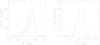 |
Fig. 2 Distribution of stellar masses (left) and visual magnitudes (right) of our targets (black line), the known M dwarf data from Swift et al. (2015,blue dash-dotted line) and Bo13 (red line). |
To estimate stellar properties, we apply the techniques introduced in Maldonado et al. (2015). Spectral types (SpT), effective temperatures, and metallicities are obtained from calibrations of the ratios of sensitive line features and their combinations. Those values are then used to determine masses, radii, and surface gravities in an empirical way. The description of the stellar parameters are provided with details in Maldonado et al. (2017), whilst we show the relevant data for the present study in Table A.1. Data for targets without observations were collected from the SIMBAD astronomical database (Wenger et al. 2000) with masses averaged from the values of stars of the same type from our sample.
In the left panel of Fig. 1 the distribution of number of spectra is shown for our targets. We observed 40 targets more than 20 times each, which is the average number of the study by Bo13 and which we consider as a lower limit necessary for the detection of planets. In the right panel, we see the distribution of spectral types ranging from M0 to M3, with a peak at approximately M1. This narrow spectral type interval was purposely chosen to minimize the number of parameters and derive meaningful statistics.
In Fig. 2 we show the distributions of stellar masses and visual magnitudes ranging from 0.30 to 0.69 M⊙, with a peak at approximately 0.5 M⊙, and 8.1 to 12.0 mag, respectively. The magnitudes of the sample targets combined with the nominal selected integration time of 900 s leads to a range of signal-to-noise ratios (S/N) at mid-wavelengths (spectral order 46) of 23 to 163 (see Table A.1).
Our distribution of stellar masses is similar to the one used for the Kepler stars by Swift et al. (2015), while the sample of the HARPS Doppler spectroscopy survey of Bo13 shows, on average, lower masses, later spectral types and visual magnitudes of up to 14 mag. In this latter case, the targets have an upper limit to the distance of 11 pc, whereas our objects show an average of 19.2 ± 8.5 pc and only ten targets closer than the 11 pc limit. The nine detected planets by Bo13 orbit stars with characteristics of M2.0 < SpT < M3.0, 0.3 <M< 0.5 M⊙, and 9.4 <V< 10.6 mag, covered by the HADES program.
2.2. Data treatment
The Data Reduction System pipeline (DRS, Lovis & Pepe 2007) of the HARPS-N instrument reduces the data using the classical optimal extraction method by Horne (1986) including bias and background subtraction and flat-fielding and delivers cosmic ray-corrected, wavelength-calibrated spectra. Furthermore, it calculates RVs using the cross-correlation function (CCF) method (Queloz 1995; Baranne et al. 1996; Pepe et al. 2002). It calculates a contrast value by multiplying an observed spectrum with a template mask. In our case, we use the mask of an M2 star, which consists of approximately 9000 wavelength intervals of 820 m s-1 width (the HARPS-N pixel size) representing line features and their depths that are less affected by blending, and avoid regions of high telluric line densities approximately 5320, 5930, 6300 and 6530 Åand are weighted to take into account their expected S/N. The CCF is fitted by the pipeline with a Gaussian function and the peak is the desired RV value. All these reduction steps are done on each of the diffraction orders of the 2D echelle spectra. The final measurements are then the flux-weighted mean of the values measured across all orders. We re-reduced the observed data with YABI (Hunter et al. 2012; Borsa et al. 2015). This tool is provided by the GAPS team and uses the same reduction steps as the DRS but giving the additional opportunity to change important values for the calculation of the CCF. YABI is mainly used to reduce the data in the same manner, and to avoid small changes made in the DRS over the years. An average RV uncertainty of 1.71 m s-1 is achieved for the YABI data set. The Geneva team (F. Pepe, priv. comm.) introduces an additional instrumental error of 0.6 m s-1 due to the uncertainty of the wavelength calibration. For more details see Cosentino et al. (2012) or the HARPS DRS manual3.
We used a further approach to derive the RVs, namely the Java-based Template-Enhanced Radial velocity Re-analysis Application (TERRA, Anglada-Escudé & Butler 2012). TERRA handles the full process of unpacking the HARPS-N archive files in the DRS and YABI output. For each order it corrects for the blaze function variability (i.e., flux) and, in a first run, performs a least-squares fit with each spectrum and the spectrum of highest S/N of each target. With this information, a co-added template including all RV-corrected input spectra of very high S/N is calculated. This is used as a reference in a second run of least-squares fitting to find the final RVs. TERRA offers the opportunity of selecting the number of orders included in the calculation of the RVs. For HARPS-N the usage from order 18 to 66 is recommended (G. Anglada-Escudé, priv. comm.) in order to minimize the RV root-mean-square (rms) of the authors examples. This idea includes the assumption that the smaller observed RV rms correspond to the smaller RV noise rms. The selected orders also correspond to the wavelength range of the M2 mask of the HARPS-N DRS. We obtain an average uncertainty of 1.03 m s-1 with our dataset.
There are known shortcomings in the way in which the DRS and YABI handle the CCF resulting from the cross-correlation with the M2 mask. A symmetric analytical function is fitted to the asymmetric CCF, and also the fit is further complicated by the appearance of side-lobes caused by numerous lines included in the mask. Also, spectral type differences between the mask and the target can affect the values of the CCF significantly, as shown by our tests with the StarSim simulator (Herrero et al. 2016). The TERRA algorithm, on the other hand, introduces further error sources by using the full spectrum including all blended lines and regions of higher telluric line density.
To verify which method delivers the most precise results for our sample, we ran a simple test for comparing the rms residuals of the RVs of each object using both methods (see Fig. 3 and Table A.1). The underlying idea is that, as already mentioned, when considering a statistically significant sample, the method that yields smaller rms of the RV measurements for the same dataset should be preferred. Even in the presence of planets and activity signals, more reliable measurements should result in smaller residuals. Also, it could be the case that the method yielding lower rms values does so due to its decreased sensitivity to stellar activity effects, and this also works in favour of improving the chances of discovering exoplanet signals, which is the main goal.
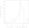 |
Fig. 3 Distribution of RV rms differences from TERRA and YABI for 62 targets. The mean value of −0.63 m s-1 is indicated by the dash-dotted line. Note that two and one outliers are not shown on the left and right extreme ends of the diagram, respectively (see Table A.1). |
The 62 stars with >1 observations show average rms values of 3.6 and 4.3 m s-1 and median rms of 2.9 and 3.4 m s-1 for TERRA and YABI pipelines, respectively. The average difference between TERRA and YABI is −0.63 m s-1 and there are only 13 targets showing larger rms values for TERRA, which do not share any similar characteristics. Given the results of this comparison, we adopt the RV data and associated error bars as derived by TERRA.
3. Simulations
To address our main questions for the mean noise and activity level of early-M dwarfs, the number of observations needed to detect a significant percentage of planets, and the overall observational strategy, we use the code described by García-Piquer et al. (2016). This code was written to simulate the outcome of the CARMENES observations after the application of the CARMENES Scheduling Tool (CAST, Garcia-Piquer et al. 2014). With the input of stellar properties such as the visual magnitude V, SpT, effective temperature, M, the observational dates and the corresponding RV uncertainties, the code generates simulated planets around the input stars and applies a search for periodicity.
3.1. Adopted occurrence rates
As further input to the code, we need to include distributions of various planetary characteristics. Many studies have already been conducted to derive such occurrence rates (Gaudi et al. 2002; Marcy et al. 2005; Naef et al. 2005; Sahu et al. 2006; Cumming et al. 2008; Bowler et al. 2010; Howard et al. 2010; Nielsen & Close 2010; Borucki et al. 2011b; Cassan et al. 2012; Howard et al. 2012; Quanz et al. 2012; Wright et al. 2012; Swift et al. 2013; Clanton & Gaudi 2014; Burke et al. 2015) including those using different kinds of methods, stellar environments and characteristics, but these are rarely focused on low-mass stars. In the following, we outline the parameter distributions available and the ones used by García-Piquer et al. (2016) and our work.
For the orbital period, the most significant and reliable statistics are provided by the Kepler survey. Among the most comprehensive studies is that of Fressin et al. (2013), who investigated 932 FGKM stars from Batalha et al. (2013) and analyzed approximately 180 planets with 0.8 <PP< 418 days and 0.8 <RP< 22 R⊕. Swift et al. (2015) focused on M dwarfs and delivered distributions of RP and PP covering 0 to 13 R⊕ and 0 to 200 days, respectively. Dressing & Charbonneau (2013, 2015) study 156 planets detected in a sample of 2543 Kepler stars with T< 4000 K with specific interest in small planets in the habitable zone, and so the parameter intervals are PP from 0.5 to 200 days and RP from 0.5 to 4 R⊕. When correcting for detection biases, all of these publications, together with Kopparapu (2013), suggest a high occurrence rate of approximately 0.5 of small planets around low-mass stars.
To describe the planet population we adopt a combination of these distributions. For planets of MP> 30 M⊕ (large Neptunes, Jupiters, Giants) and 0.5 <PP< 418 days we follow Fressin et al. (2013) and for MP< 30 M⊕ (Earths, Super-Earths and small Neptunes) and 0.5 <PP< 200 days we follow Dressing & Charbonneau (2015). This division was also applied by a similar simulation done by Sullivan et al. (2015) for stars ranging from 0.15 to 0.78 M⊙ and takes into account the lower probability of planet occurrence on short periods. Additionally, in our simulation, we use the constraint of avoiding the generation of planets in the same system with period ratios <1.3. We use the following equation (see bottom panel of Fig. 4):  (1)For planets with MP> 30 M⊕ we use a = −4, b = 2.205, c = −0.835, and D = 3.13 and for MP< 30 M⊕ we use a = −2, b = 0.954, c = −0.637, and D = 1.04, respectively.
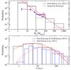 |
Fig. 4 Top: planet mass distribution assumed for our simulations. Solid bars show the probability distribution computed from planet rates given by Mayor et al. (2011). Dashed bars show the scaled distribution for M dwarf host stars following the exoplanet statistics from Dressing & Charbonneau (2013). Our fit to this scaled distribution is plotted in red. These distributions are normalized between 3 and 1000 M⊕. We show the distribution of minimum masses of the 155 planets from Mayor et al. (2011, dashed red line and dots), and the 81 theoretical solutions from Bo13 (dashed blue line and dots).Bottom: orbital period distributions corresponding to planet rates in Fressin et al. (2013, blue) and Dressing & Charbonneau (2015, black) used for planets with masses above and below 30 M⊕, respectively. Solid and dashed red lines indicate the functional fits to these normalized distributions. |
For the distribution of MP, which is the relevant parameter in a spectroscopic survey, we face the problem that the Kepler mission statistics are based on measurements of RP, which is the observable parameter resulting from transit modeling. Current observations show that the relationship between MP and RP is very scattered and far from being univocally defined. For this reason, we prefer to employ the statistical distribution of planet masses coming from spectroscopic observations. Mayor et al. (2011) use data of approximately 1200 inactive late-F to late-K dwarfs resulting in the detection of 155 confirmed planets in 102 systems. Bo13 provide the only significant statistics of planets around M dwarfs considering MP ranging from 1 to 104M⊕ and periods PP ranging from 1 to 104 days from the detection of 9 planets in 102 targets. For our simulations we adopt the results of Mayor et al. (2011), with a scaling factor for MP> 30 M⊕ of 1.5% following Dressing & Charbonneau (2013) in order to match the lower frequency of large planets around the low-mass stars. We reach up to 1000 M⊕ and extrapolate the fit below 3 M⊕ down to 1 M⊕. Although we expect that planets with lower masses are very abundant, their statistical distribution is not sufficiently well constrained and it is very unlikely for our simulations or the observational HADES program to detect them. We use the following equation (see top panel of Fig. 4):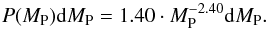 (2)In this work we use the described functional fits instead of the tables given in the publications for MP and PP in order to approximately reproduce the expected behaviour of the probability distributions. The solutions for M-type stars found by us are still unclear and should be taken with some caution given the uncertainties of planet ratio tables, yet we hope to be able to contribute to this interesting question once the HADES program is finished.
In the comparison of the distributions of published MPsini by Mayor et al. (2011) and Bo13 and the models used, we see the observational bias towards more massive planets, where the authors essentially detect all planets more massive than 20 M⊕, but miss the less massive ones. We show a plot of PP vs. MPsini of the data of the two mentioned publications in Fig. 5. The values from the 155 confirmed planets by Mayor et al. (2011) are relatively evenly distributed over the plot apart from the technically inaccessable region of low MPsini and long PP and the region of high MPsini and low PP not populated by planets. The data of the 81 best theoretical solutions for planets from Bo13 show few planets beyond 100 M⊕ and 100 days, such as their nine detected planets.
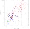 |
Fig. 5 Orbital period against minimum mass for 81 best theoretical solutions for the targets of Bo13 (blue dots) and the 155 confirmed planets of Mayor et al. (2011, red diamonds). The large blue and green dots indicate the nine planets detected by Bo13 and the two planets detected by our group (Affer et al. 2016), respectively. The grid constructed from dashed and dotted lines is for better comparison with Fig. 12. |
Besides the distributions for PP and MP, we use the probability distributions of the sine wave of the inclination (0 <i< 90°) and the argument of periastron (0 <ω< 360°), which we assume to be flat, and the eccentricities (0 <εP< 1) distributed following Kipping (2013) for all stellar types with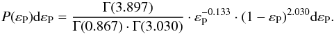 (3)The multiplicity distribution of planets around M dwarfs can be taken from Dressing & Charbonneau (2015) and the Kepler Object of Interest statistics for 1135 stars and show 58.8, 26.6, 8.6, 4.4, 1.4, 0.6, 0.6% for stars with 1, 2, ..., 7 planets. Assuming that every star has a planet, we thereby distribute, on average, 1.70 planets per star, which is in the range of the values stated by Gaidos et al. (2014) and Dressing & Charbonneau (2015).
The construction of the parent distribution of planets is complex. This is needed since every survey has its own properties and bias. We choose a combination of various approaches and biases, since the real distribution is unknown and we do not consider it crucial for our goal to compute the efficiency in detecting small planets and not only their absolute numbers.
3.2. Simulation of observations
To minimize numerical errors, we ran simulations considering 1000 scenarios, that is, different distributions of planets. On average, the realizations produce 128.1 ± 8.3 planets around our 78 sample stars. Of them, 123.0 ± 8.3 (96.0%) are terrestrial (i.e., Earths and Super-Earths with MP< 10 M⊕), 3.0 ± 1.6 (2.4%) are transiting planets (cos i< ), and 27.3 ± 4.9 (21.3%) are located in the habitable zone of their respective host star. For the latter, we use the moist and maximum greenhouse case for the inner and outer habitable zones following Kopparapu et al. (2013).
For each of the realizations, we use the underlying planet population to create a simulated time series of RV measurements. We employ the real dates of our observations and the RV uncertainties found by TERRA pipeline. The 54 stars with more than five observations show mean and median observational RV rms of 4.0 and 3.1 m s-1, respectively. The simulations of the RVs consider the contributions from the injected planets and the observational uncertainties, but lack the effects introduced by magnetic activity or other additional noise sources.
These values, however, are not completely representative of the magnetic activity noise since part of the signal corresponds to correlated (periodic) contribution that is usually removed during the detailed analysis by means of, for example, photometric time series or measurements of periodicities in activity indicators such as Hα and Ca ii. For a quantitative estimate of this contribution to the RV rms we employ the identified periodicities associated to stellar rotation, differential rotation, and their harmonics (Suárez Mascareño et al., in prep.), which reduce the RV rms of the stars by 84%, on average (not considering the absolute RV rms). By also removing any long-term trends and applying a 3σ-clipping to the RV rms (rejecting TYC 2703-706-1 and NLTT 21156 because of their outlier values), we are left with a mean and median observational RV rms of 3.0 and 2.8 m s-1, respectively, for the remaining 52 target stars.
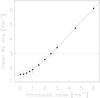 |
Fig. 6 Relationship between the additional white noise introduced quadratically in the simulated RV values and the resulting RV rms for 52 target stars. The dots indicate the probed values, whereas the full drawn line is the best polynomial fit. The dashed dotted line indicates the mean observed value (without correlated activity jitter) of 3.0 m s-1. |
To match this mean value, we searched for the correlation between a white noise contribution added in quadrature and the resulting mean RV rms for our simulation (see Fig. 6). This was found to be  (4)with a = 1.506 ± 0.241, b = 0.141 ± 0.552, c = 0.256 ± 0.333, d = −0.037 ± 0.0.068, and e = 0.002 ± 0.004.
For our mean value of 3.0 m s-1, we find an additional noise of 2.6 m s-1. Note that this added noise is the combination of three sources: 1) the mean instrumental drift of 1.0 m s-1; 2) the additional instrumental error of 0.6 m s-1 described above; and 3) the uncorrelated magnetic activity (or RV) jitter (Martín et al. 2006; Prato et al. 2008). If these noise contributions are treated as uncorrelated, we obtain a mean value for the RV jitter associated to stellar activity of 2.3 m s-1.
The simulated RVs so far consist of the observational uncertainties and the contribution of the simulated planets for each target. If we were to quadratically add this mean noise of 2.6 m s-1 to each target, we would end up with the same mean RV rms but not with the same RV rms distribution. Furthermore, we would underestimate the number of targets with RV rms below the mean jitter value. Therefore, in a case where the simulated RV rms of a target is smaller than its observed one, we quadratically add a noise term to the simulations to match the observational RV rms (converted by Eq. (4)). If the simulated RV rms of a target is larger than its observed one, we do not add any noise. We thereby create a similar simulated RV rms distribution as for our observations.
We show the RV rms distributions of the 52 stars in Fig. 7. The red curve indicates the distribution as observed ranging from 1.1 to 6.0 m s-1, while the blue curve shows the wide distribution simulated initially (note the logarithmic scale). The black curve is therefore the final RV rms distribution after adding the noise to each target in every iteration to reach its observed RV rms (without the correlated activity jitter). The simulated targets with RV rms lower than 1.1 m s-1 are due to the Gaussian distribution applied and reach down to approximately 0.5 m s-1. The targets with RV rms larger than 6 m s-1 were distributed by the simulation and not modified. By keeping the RV rms of every target constant we introduce additional error sources: 1) the RV rms of different spectral types are fixed, but we focus only on a number of different types and their mean RV rms, ranging from 2.0 to 3.7 m s-1, do not differ significantly from the overall one; 2) the RV rms of targets with different numbers of observations are fixed, but the RV rms for targets with 40, 70, 90, and 100 observations, with 3.2, 3.2, 3.3, and 3.1 m s-1, respectively, are in agreement with the overall mean RV rms. We note that the planetary candidates detected by the HADES program so far show host stars with RV rms of 5.6 and 4.2 m s-1 (including the planetary signals).
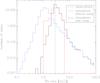 |
Fig. 7 Histogram of RV rms for 52 stars with more than five observations and a 3σ-clipping of the RV rms using observations (red), initial (blue) and final (black) simulations. The initial RV rms distribution does not include any activity jitter, whereas the final distribution includes it by quadratically adding the RV rms as observed for each individual target. For the simulations, we have uncertainties of the histogram values in the order of (0.92NS)0.5 and (0.94NS)0.5 for the black and blue curve. respectively, with NS being the number of stars. They are not shown for reason of clarity. |
We then use the Generalized Lomb-Scargle periodogram (GLS, Zechmeister & Kürster 2009), which includes error-weighting and the consideration of an RV offset, in order to search for the planets in our RV data. As significance threshold, we use the power corresponding to a given False Alarm Probability (FAP), which we estimate and calculate from the Horne number of independent frequencies (Horne & Baliunas 1986). An injected planet is detected, if 1) its period is connected to the highest peak of the GLS periodogram; 2) its FAP is below the usual threshold of 0.1%, corresponding to a 99.9% probability level and 3) its frequency f =  is located inside the frequency resolution
  described by Zechmeister & Kürster (2009), where T is the observational time span of the target. The subtraction of the most significant signal (assuming a Keplerian fit) and subsequent search for additional signals is repeated until no relevant periodicity is left. In the Keplerian fits and analysis of the residuals we do not consider linear trends and adopt circular orbits, which is valid at least for short periods (see e.g., Marcy et al. 2014). For further details of the simulating process, we refer to García-Piquer et al. (2016).
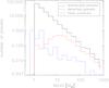 |
Fig. 8 Histogram of minimum masses of the distributed planets around our 78 targets (black line). The red curve indicates the respective distribution of detected planets in our simulation comparable to the observations, and the blue line shows the false positives. Errors are in the order of (0.97NP)0.5 for all planets, (1.00NP)0.5 for the detected ones, and (0.79NP)0.5 for the false positives, respectively, NP is the number of planets. |
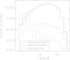 |
Fig. 9 Histogram of orbital periods of distributed (black) and detected (red) planets. Uncertainties are in the order of (0.96NP)0.5 for all planets and (0.99NP)0.5 for the detected ones, respectively. Also shown is the distribution of false positives (blue), with an uncertainty of (0.90NP)0.5. |
The distributions of MPsini and PP are shown in Figs. 8 and 9 with the distributed planets represented by the black lines and the detected planets by the red lines. Also shown are the distributions of false positive signals in blue. As already seen in the comparison of theoretical models and observational data in Fig. 4, all planets in our simulations more massive than 20 M⊕ are detected. The highest detection rates we find for planets between 5 and 25 M⊕, whereas for planets below 3 M⊕, the false positive rate is relatively high. The values here also go below our set limit of 1 M⊕, since the GLS detects them without considering our limit. In the case of the orbital periods, the highest rate is found for 10–25 days and the detection curve obviously shows some bias favoring shorter period planets. In this range below three days, however, the false positive signals are as numerous as generated planets, whereas they are negligible for longer periods. If we integrate across all the parameters (i.e., area below the red lines in both Figs. 8 and 9), our simulations show that the observations of the HADES program analyzed here should permit the detection of 2.4 ± 1.5 planets (1.9% detection rate). This is in agreement with the three planet detections announced by Affer et al. (2016) and Perger et al. (in prep.). Regarding the distribution of the simulated RV amplitudes, Fig. 10 shows a maximum (black curve) at approximately 0.4 m s-1 and values ranging from 0.01 to 100 m s-1. The decrease of the distribution at low amplitudes is a consequence of the limit of 1 M⊕ applied to the planets and not a physical effect. Planets with amplitudes K> 5 m s-1 are detected easily as seen by the curve of detected planets (black dash-dotted line). The false-positive rate (in blue) rises very quickly for amplitudes <2 m s-1, which is below the introduced mean RV jitter of 2.7 m s-1.
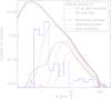 |
Fig. 10 Histogram of RV amplitudes K, where the distribution for all simulated planets is shown by the solid black line with uncertainties of (0.97NP)0.5. We show the outcome of the simulations comparable to our observations (uneven 34.3 observations per star) of Sect. 3.2, where the black dash-dotted line indicates the planet detections and the blue histogram the false positives with uncertainties of (0.91NP)0.5. The red curves indicate the distributions for detected planets for 20 (bottom), and 200 (top) observations per star, the red dash-dotted line for even 35 observations per star (see Sect. 3.3). Uncertainties for all the curves of detected planets are in the order of (0.98NP)0.5. |
If we compare the outcome of the simulations with Bo13 and our own planetary candidates, the mean minimum masses and mean periods found for all planets are located in the described maxima of the curves. It is notable, however, that the detected planets by Bo13 show a mean amplitude of 4.7 m s-1, which is almost double that of our planets with 2.6 m s-1 and improves their detectability.
3.3. Number of observations
With the additional noise added to each individual target as described, we investigate the relationship between the mean number of observation per target and the efficiency in the detection of planets. We ran simulations for the 78 targets using the same number of observations, including 20, 35, 50, 70, 90, 120, 150, and 200 obs/star. We constructed our own schedules cutting out some already made observations and/or adding additional future observations matching the usual distribution of observations of our teams (EXOTEAM and GAPS-M) in the past semesters. Uncertainties are the ones observed with TERRA, or Gaussian errors randomly distributed around the mean TERRA uncertainty of that object (or objects of same spectral type, see Table A.1), respectively.
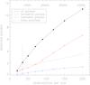 |
Fig. 11 Relationship between the amount of all detected planets and the number of observations per star for the 78 sample stars (black dots, uncertainty (0.92NP)0.5), of the terrestrial planets (red squares, (0.62NP)0.5), the habitable planets (blue triangles, (0.95NP)0.5) and the false positives (black dashed line, (1.17NP)0.5). We indicate at the top the number of total observation times. With the 891 h total observation time and 34.3 observations per star on average of our survey (vertical black dashed line). We detect approximately 2.1 planets resembling the detection rate for evenly distributed 35 observations per star. |
In addition to the results explained in Sect. 3.2, Fig. 10 shows the distribution of the RV semi-amplitudes K of the detected planets for various fixed observations per star, including 20, 35, and 200. Comparing the curve drawn by the simulations using an even 35 obs/star for all stars (dash-dotted red line) with the curve drawn by the simulations of our observational case (dash-dotted black line) with unevenly distributed 34.3 obs/star on average, we observe a shift to smaller amplitudes of the curve, equivalent to an improvement in the detection of planets with such characteristics. This is obvious, since we are only able to detect those lower amplitude planets with a significantly higher number of observations. The increased detection of signals with K< 1 m s-1 are the false positives included in the diagram.
The integrated number of planets of different types as a function of the number of observations is shown in Fig. 11. We reach a similar result as for our actual observations with 34.3 obs/star and 891 h of total observation time (2.4 planets detected) with an evenly distributed 35 obs/star. Spreading observations among all targets is almost as efficient as focusing on promising targets. As expected, the curves approximately follow a square root function. We can compare the results with the ones found for the CARMENES survey by García-Piquer et al. (2016), who use an average of approximately 100 to 110 obs/star and detect approximately 5% of their planets adding an additional RV jitter of 3 m s-1. In our case, with a mean white noise contribution of 2.6 m s-1 we also detect some 5% of the distributed planets for the same amount of observations per star. Bo13 detect approximately 6% of the planets, if we use the same distribution rate as in our study and put 160.8 planets around their 102 host stars. Although they use only 20 HARPS spectra per target, they were able to pre-select and clean their sample using a large number of lower resolution spectra from the ELODIE (OHP, France) and FEROS (La Silla, Chile) spectrographs. And, as already described, the planets detected by Bo13 show large mean RV amplitudes, which do not seem to be present in our data.
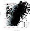 |
Fig. 12 Minimum masses vs. orbital periods of all the simulated planets (black line) and their distribution in percent in various subregions of the plot (red numbers) indicated by the dotted grid. From light gray (200 obs/star) to black (20 obs/star), we show the distributions of every detected planet of the 1000 simulations as indicated in the legend. |
In Fig. 12 we show MPsini vs. PP for all distributed and detected planets. The black line shows the limits of all planets distributed around the 78 sample stars. We also indicate in red the percentage of planets located inside a logarithmic grid made from dotted lines. From black to light gray we show the distributions of every detected planet of the 1000 simulations from 20 to 200 obs/star as marked by the color legend, respectively. As indicated by the red marked numbers in the grid, the planets of our simulations are distributed approximately 1.5 M⊕ and 15 days, while the detected planets for each number of observations per star are located along a line marked by the least massive planets. The distribution for 35 obs/star agrees well with the curves obtained by our observations in Figs. 8 and 9. The false positive planetary detections are visible in the area of lower masses and longer periods.
Comparing the results to the data in Fig. 5, many planets and planetary candidates are located along the line of detection, but only a small number in the center of distributed planets. As a rough comparison, most planets or planetary candidates by Mayor et al. (2011) and Bo13 are detectable with 35 to 50 obs/star.
3.4. Survey strategy
We further investigate the observational strategies by keeping the total duration of the survey constant and by varying the number of target stars and the subsequent number of observations per star. In short, we wanted to determine whether it is more efficient to observe fewer targets many times or more targets fewer times.
We consider ten stars of our stellar sample as a base, selected in such a way that the spectral type distribution is similar to the original 78 star sample: two M0, M0.5, M1, and M1.5 stars and one M2 and M2.5 star (marked in Table A.1). The sub-sample shows a mean and median RV rms of 2.9 and 3.2 m s-1. We consider the similarity to the spectral type distribution and the overall RV rms as very important for the results of the simulations to be applicable to our entire sample. We do the simulations including the sample various times using 20 to 150 stars as shown in Table 1. For the maximum number of targets, we distribute 246.2 ± 11.2 planets. We keep the total survey times of 800, 1200, and 1600 h fixed and calculate the corresponding number of observations per target for each number of stars using the exposure time of 900 s. We employ the observational uncertainties and the additional noise level used for each individual target as explained in Sect. 3.2. We then compare the number of detected planets as a function of the number of targets for a given total observation time in Fig. 13.
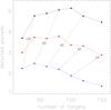 |
Fig. 13 Relationship between the number of detected planets of our simulations and the number of stars used for the survey. For a given total observation time of 800 (blue), 1200 (red) and 1600 h (black) we simulated 20 to 150 stars with 16 to 240 observations per star following Table 1. In the diagram, we connect points with the same number of observations per star using dash-dotted lines. Uncertainties are in the order of 1.4, 1.8, and 2.1 planets for the blue, red and black curves, respectively. |
Numbers of observations per target for different numbers of target stars for three fixed total survey times of 800, 1200, and 1600 h.
As expected, the total number of target stars that maximizes the number of detected planets varies with the total survey time. The peak is located at approximately 90–120 targets for 1600 h, and it progressively shifts to lower numbers of targets as the total survey time decreases, reaching a value of 30–50 for 800 h. We can estimate the maximum planet detection as a function of the number of observations per star. We connect measurements of same number of observations per target for different total observation times by the dash-dotted line. In light of the plot, we can infer the position of the maximum of the curves and find that such value is approximately 40–60 observations per star for a survey of early-M stars distributed as the targets of the HADES program. Thus, for 800, 1200, and 1600 h of observation (i.e., 100, 150 and 200 observing nights), the optimum number of targets with exposure times of 900 s to survey is, approximately, 46, 69 and 92 targets, respectively. Surveys adopting a different strategy will suffer from diminished detection efficiency.
4. Conclusions
We present the global analysis of the 2674 spectra of our HADES program, in which we have been monitoring (and continue to observe) 78 M0 to M3-type stars for the last four years with HARPS-N high-resolution Doppler spectroscopy. We compare the two reduction pipelines DRS/YABI and TERRA and find significant differences in the mean RV variations for our stars with 4.3 and 3.6 m s-1, respectively, and 79% of the targets showing lower variations for TERRA. Using the criterion that minimum rms value is associated to a lower level of instrumental and stellar noise, we conclude that the TERRA results are to be preferred as they appear to extract RVs with the best accuracy and/or are less affected by stellar magnetic activity. Following such a strategy, careful measurements of RV and subsequent critical analysis has allowed the discovery and recent announcement of a two-planet system of super-Earths by our team (Affer et al. 2016).
Here we also investigate the stellar noise properties of our early M dwarf sample and, as a consequence, produce an estimate of the planet detection rate that we compare with our results. We have performed a series of simulations using state-of-the-art planet occurrence statistics applied to our stellar sample and the actual observation times of our survey. Comparison of the predicted RV variations with the real measurements yields a mean stellar noise level of 2.6 m s-1. Accounting for the typical HARPS instrumental errors and drift values, we find an RV jitter level associated to stellar activity of 2.3 m s-1. In our simulations we keep the RV rms of each individual target constant since the distribution of the RV rms values would be significantly broader in cases where we use the assumption of a mean noise level for all stars. We predict that our survey should have been able to detect significant signals from 2.4 ± 1.5 planets, which is an approximate estimate but in good agreement with the announced discovery of two exoplanets so far. The results show that planets with MP> 5 M⊕, K> 2 m s-1 and 10 <PP< 25 days are best detected which is confirmed by both the results from Bo13 and the HADES program. For detections with masses, periods and amplitudes smaller than the mentioned values, the false positive rate is significant.
With our simulations we also study the detection rate of planets while increasing the number of obs/star from 20 to 200. This produces an increase in the detection rate by an order of magnitude and with 95 obs/star, we are able to detect approximately 5% of the distributed planets. We also note, that most of the available planet candidate signals from Bo13 can be detected with approximately 35–50 obs/star, whereas with less observations, the level of false positive detections is significantly higher. Those numbers are also necessary for the detection of planets with amplitudes of approximately 2 m s-1. Results indicate that we best detect planets with values approximately ten days and >10 M⊕, while the simulated planets are distributed approximately 1.5 M⊕ and 15 days. Although not affecting the total number of detections, we can numerically demonstrate that it is more efficient to concentrate on promising targets (those with conspicuous signals) than to distribute observations equally amongst all targets if searching for low-amplitude signals.
A further application of our simulation scheme is to assess the optimum number of targets (and observations per targets) in the case of a time-limited survey, which is expected to be the most frequent scenario. Our analysis shows that the most efficient strategy is to keep the average number of observations per target constant at approximately a value of 50. This is, of course, for the case of an early M-dwarf sample and exposure times of 900 s. Then, given an expected amount of observing time, the optimum number of targets in the survey sample can be immediately calculated.
We note that the rates of detected planets mentioned in this study may be underestimated owing to the fact that we could not correct for the correlated magnetic activity in all our targets. We include simulated host stars with planetary companions reaching RV rms values beyond the 6 m s-1 observed by our HADES program. Another note of caution should be added here concerning the still relatively large uncertainties in the exoplanet statistics around M dwarfs, which we aim to reduce with the HADES program. However, the planet population seems to be sufficiently well established to reach conclusions on the optimal survey design. We therefore suggest that surveys optimize their strategy in light of our results to avoid a diminished detection efficiency.
Acknowledgments
The HARPS-N Project is a collaboration between the Astronomical Observatory of the Geneva University (lead), the CfA in Cambridge, the Universities of St. Andrews and Edinburgh, the Queens University of Belfast, and the TNG-INAF Observatory. We made use of the SIMBAD database, operated at CDS, Strasbourg, France. Thanks to Guillem Anglada-Escudé for the TERRA reduction pipeline and to the YABI project. GAPS acknowledges support from INAF through the “Progetti Premiali” funding scheme of the Italian Ministry of Education, University, and Research. M.P., I.R., J.C.M., A.R., E.H., and M.L. acknowledge support from the Spanish Ministry of Economy and Competitiveness (MINECO) through grant ESP2014-57495-C2-2-R. J.I.G.H. acknowledges financial support from the Spanish Ministry of Economy and Competitiveness (MINECO) under the 2013 Ramón y Cajal program MINECO RYC-2013-14875, and A.S.M., J.I.G.H., and R.R.L. also acknowledge financial support from the Spanish ministry project MINECO AYA2014-56359-P.
References
- Affer, L., Micela, G., Damasso, M., et al. 2016, A&A, 593, A117 [NASA ADS] [CrossRef] [EDP Sciences] [Google Scholar]
- Amado, P. J., Quirrenbach, A., Caballero, J. A., et al. 2013, in Highlights of Spanish Astrophysics VII, eds. J. C. Guirado, L. M. Lara, V. Quilis, & J. Gorgas, 842 [Google Scholar]
- Anglada-Escudé, G., & Butler, R. P. 2012, ApJS, 200, 15 [NASA ADS] [CrossRef] [Google Scholar]
- Baranne, A., Queloz, D., Mayor, M., et al. 1996, A&AS, 119, 373 [NASA ADS] [CrossRef] [EDP Sciences] [Google Scholar]
- Basri, G., Walkowicz, L. M., & Reiners, A. 2013, ApJ, 769, 37 [NASA ADS] [CrossRef] [Google Scholar]
- Batalha, N. M., Rowe, J. F., Bryson, S. T., et al. 2013, ApJS, 204, 24 [NASA ADS] [CrossRef] [Google Scholar]
- Bonfils, X., Forveille, T., Delfosse, X., et al. 2005, A&A, 443, L15 [NASA ADS] [CrossRef] [EDP Sciences] [Google Scholar]
- Bonfils, X., Mayor, M., Delfosse, X., et al. 2007, A&A, 474, 293 [NASA ADS] [CrossRef] [EDP Sciences] [Google Scholar]
- Bonfils, X., Delfosse, X., Udry, S., et al. 2013, A&A, 549, A109 [NASA ADS] [CrossRef] [EDP Sciences] [Google Scholar]
- Borsa, F., Scandariato, G., Rainer, M., et al. 2015, A&A, 578, A64 [NASA ADS] [CrossRef] [EDP Sciences] [Google Scholar]
- Borucki, W. J., Koch, D. G., Basri, G., et al. 2011a, ApJ, 728, 117 [NASA ADS] [CrossRef] [Google Scholar]
- Borucki, W. J., Koch, D. G., Basri, G., et al. 2011b, ApJ, 736, 19 [NASA ADS] [CrossRef] [Google Scholar]
- Bowler, B. P., Johnson, J. A., Marcy, G. W., et al. 2010, ApJ, 709, 396 [NASA ADS] [CrossRef] [Google Scholar]
- Burke, C. J., Christiansen, J. L., Mullally, F., et al. 2015, ApJ, 809, 8 [NASA ADS] [CrossRef] [Google Scholar]
- Butler, R. P., Johnson, J. A., Marcy, G. W., et al. 2006, PASP, 118, 1685 [NASA ADS] [CrossRef] [Google Scholar]
- Cassan, A., Kubas, D., Beaulieu, J.-P., et al. 2012, Nature, 481, 167 [NASA ADS] [CrossRef] [Google Scholar]
- Clanton, C., & Gaudi, B. S. 2014, ApJ, 791, 91 [NASA ADS] [CrossRef] [Google Scholar]
- Cosentino, R., Lovis, C., Pepe, F., et al. 2012, SPIE Conf. Ser., 8446, 1 [Google Scholar]
- Covino, E., Esposito, M., Barbieri, M., et al. 2013, A&A, 554, A28 [NASA ADS] [CrossRef] [EDP Sciences] [Google Scholar]
- Cumming, A., Butler, R. P., Marcy, G. W., et al. 2008, PASP, 120, 531 [CrossRef] [Google Scholar]
- Delfosse, X., Forveille, T., Mayor, M., et al. 1998, A&A, 338, L67 [Google Scholar]
- Desidera, S., Sozzetti, A., Bonomo, A. S., et al. 2013, A&A, 554, A29 [NASA ADS] [CrossRef] [EDP Sciences] [Google Scholar]
- Dressing, C. D., & Charbonneau, D. 2013, ApJ, 767, 95 [NASA ADS] [CrossRef] [Google Scholar]
- Dressing, C. D., & Charbonneau, D. 2015, ApJ, 807, 45 [NASA ADS] [CrossRef] [Google Scholar]
- Fressin, F., Torres, G., Charbonneau, D., et al. 2013, ApJ, 766, 81 [NASA ADS] [CrossRef] [Google Scholar]
- Gaidos, E., Mann, A. W., Lépine, S., et al. 2014, MNRAS, 443, 2561 [NASA ADS] [CrossRef] [Google Scholar]
- Garcia-Piquer, A., Guàrdia, J., Colomé, J., et al. 2014, in Software and Cyberinfrastructure for Astronomy III, Proc. SPIE, 9152, 915221 [CrossRef] [Google Scholar]
- García-Piquer, A., Morales, J.-C., Ribas, I., et al. 2016, A&A, submitted [Google Scholar]
- Gaudi, B. S., Albrow, M. D., An, J., et al. 2002, ApJ, 566, 463 [NASA ADS] [CrossRef] [Google Scholar]
- Gizis, J. E., Monet, D. G., Reid, I. N., et al. 2000, AJ, 120, 1085 [NASA ADS] [CrossRef] [Google Scholar]
- Hawley, S. L., Gizis, J. E., & Reid, I. N. 1996, AJ, 112, 2799 [NASA ADS] [CrossRef] [Google Scholar]
- Herrero, E., Ribas, I., Jordi, C., et al. 2016, A&A, 586, A131 [NASA ADS] [CrossRef] [EDP Sciences] [Google Scholar]
- Horne, K. 1986, PASP, 98, 609 [NASA ADS] [CrossRef] [EDP Sciences] [Google Scholar]
- Horne, J. H., & Baliunas, S. L. 1986, ApJ, 302, 757 [NASA ADS] [CrossRef] [Google Scholar]
- Howard, A. W., Marcy, G. W., Johnson, J. A., et al. 2010, Science, 330, 653 [NASA ADS] [CrossRef] [PubMed] [Google Scholar]
- Howard, A. W., Marcy, G. W., Bryson, S. T., et al. 2012, ApJS, 201, 15 [NASA ADS] [CrossRef] [Google Scholar]
- Howard, A. W., Marcy, G. W., Fischer, D. A., et al. 2014, ApJ, 794, 51 [Google Scholar]
- Hunter, A. A., Macgregor, A. B., Szabo, T. O., Wellington, C. A., & Bellgard, M. I. 2012, RESEARCH Open Access Yabi: An online research environment for grid, high performance and cloud computing [Google Scholar]
- Kipping, D. M. 2013, MNRAS, 434, L51 [NASA ADS] [CrossRef] [Google Scholar]
- Kiraga, M., & Stepien, K. 2007, Acta Astron., 57, 149 [NASA ADS] [Google Scholar]
- Kopparapu, R. K. 2013, ApJ, 767, L8 [NASA ADS] [CrossRef] [Google Scholar]
- Kopparapu, R. K., Ramirez, R., Kasting, J. F., et al. 2013, ApJ, 765, 131 [NASA ADS] [CrossRef] [Google Scholar]
- Lovis, C., & Pepe, F. 2007, A&A, 468, 1115 [NASA ADS] [CrossRef] [EDP Sciences] [Google Scholar]
- Lovis, C., Mayor, M., Pepe, F., et al. 2006, Nature, 441, 305 [NASA ADS] [CrossRef] [PubMed] [Google Scholar]
- Maldonado, J., Affer, L., Micela, G., et al. 2015, A&A, 577, A132 [NASA ADS] [CrossRef] [EDP Sciences] [Google Scholar]
- Maldonado, J., Scandariato, G., Stelzer, B., et al. 2017, A&A, 598, A27 (Paper III) [NASA ADS] [CrossRef] [EDP Sciences] [Google Scholar]
- Marcy, G. W., & Butler, R. P. 1996, ApJ, 464, L147 [NASA ADS] [CrossRef] [Google Scholar]
- Marcy, G. W., Butler, R. P., Vogt, S. S., Fischer, D., & Lissauer, J. J. 1998, ApJ, 505, L147 [NASA ADS] [CrossRef] [Google Scholar]
- Marcy, G., Butler, R. P., Fischer, D., et al. 2005, Prog. Theor. Phys. Suppl., 158, 24 [NASA ADS] [CrossRef] [Google Scholar]
- Marcy, G. W., Isaacson, H., Howard, A. W., et al. 2014, ApJS, 210, 20 [NASA ADS] [CrossRef] [Google Scholar]
- Martín, E. L., Guenther, E., Zapatero Osorio, M. R., Bouy, H., & Wainscoat, R. 2006, ApJ, 644, L75 [NASA ADS] [CrossRef] [Google Scholar]
- Mayor, M., & Queloz, D. 1995, Nature, 378, 355 [NASA ADS] [CrossRef] [Google Scholar]
- Mayor, M., Pepe, F., Queloz, D., et al. 2003, The Messenger, 114, 20 [NASA ADS] [Google Scholar]
- Mayor, M., Udry, S., Lovis, C., et al. 2009, A&A, 493, 639 [NASA ADS] [CrossRef] [EDP Sciences] [Google Scholar]
- Mayor, M., Marmier, M., Lovis, C., et al. 2011, A&A, submitted [arXiv:1109.2497] [Google Scholar]
- Naef, D., Mayor, M., Beuzit, J.-L., et al. 2005, in 13th Cambridge Workshop on Cool Stars, Stellar Systems and the Sun, eds. F. Favata, G. A. J. Hussain, & B. Battrick, ESA SP, 560, 833 [Google Scholar]
- Nielsen, E. L., & Close, L. M. 2010, ApJ, 717, 878 [NASA ADS] [CrossRef] [Google Scholar]
- Noyes, R. W., Hartmann, L. W., Baliunas, S. L., Duncan, D. K., & Vaughan, A. H. 1984, ApJ, 279, 763 [NASA ADS] [CrossRef] [Google Scholar]
- Pepe, F., & Lovis, C. 2008, in 2007 ESO Instrument Calibration Workshop, eds. A. Kaufer, & F. Kerber, 375 [Google Scholar]
- Pepe, F., Mayor, M., Galland, F., et al. 2002, A&A, 388, 632 [NASA ADS] [CrossRef] [EDP Sciences] [Google Scholar]
- Pepe, F., Molaro, P., Cristiani, S., et al. 2014, Astron. Nachr., 335, 8 [NASA ADS] [CrossRef] [Google Scholar]
- Prato, L., Huerta, M., Johns-Krull, C. M., et al. 2008, ApJ, 687, L103 [NASA ADS] [CrossRef] [Google Scholar]
- Quanz, S. P., Lafrenière, D., Meyer, M. R., Reggiani, M. M., & Buenzli, E. 2012, A&A, 541, A133 [NASA ADS] [CrossRef] [EDP Sciences] [Google Scholar]
- Queloz, D. 1995, in New Developments in Array Technology and Applications, eds. A. G. D. Philip, K. Janes, & A. R. Upgren, IAU Symp., 167, 221 [Google Scholar]
- Quirrenbach, A., Amado, P. J., Caballero, J. A., et al. 2014, SPIE Conf. Ser., 9147, 1 [Google Scholar]
- Rivera, E. J., Lissauer, J. J., Butler, R. P., et al. 2005, ApJ, 634, 625 [NASA ADS] [CrossRef] [Google Scholar]
- Sahu, K. C., Casertano, S., Bond, H. E., et al. 2006, Nature, 443, 534 [NASA ADS] [CrossRef] [PubMed] [Google Scholar]
- Santos, N. C., Bouchy, F., Mayor, M., et al. 2004, A&A, 426, L19 [NASA ADS] [CrossRef] [EDP Sciences] [Google Scholar]
- Sullivan, P. W., Winn, J. N., Berta-Thompson, Z. K., et al. 2015, ApJ, 809, 77 [NASA ADS] [CrossRef] [Google Scholar]
- Swift, J. J., Johnson, J. A., Morton, T. D., et al. 2013, ApJ, 764, 105 [NASA ADS] [CrossRef] [Google Scholar]
- Swift, J. J., Montet, B. T., Vanderburg, A., et al. 2015, ApJS, 218, 26 [NASA ADS] [CrossRef] [Google Scholar]
- Udry, S., Mayor, M., Benz, W., et al. 2006, A&A, 447, 361 [NASA ADS] [CrossRef] [EDP Sciences] [Google Scholar]
- Udry, S., Bonfils, X., Delfosse, X., et al. 2007, A&A, 469, L43 [NASA ADS] [CrossRef] [EDP Sciences] [Google Scholar]
- Wenger, M., Ochsenbein, F., Egret, D., et al. 2000, A&AS, 143, 9 [NASA ADS] [CrossRef] [EDP Sciences] [Google Scholar]
- West, A. A., Hawley, S. L., Bochanski, J. J., et al. 2008, AJ, 135, 785 [NASA ADS] [CrossRef] [Google Scholar]
- West, A. A., Weisenburger, K. L., Irwin, J., et al. 2015, ApJ, 812, 3 [NASA ADS] [CrossRef] [Google Scholar]
- Wright, J. T., Marcy, G. W., Howard, A. W., et al. 2012, ApJ, 753, 160 [NASA ADS] [CrossRef] [Google Scholar]
- Zechmeister, M., & Kürster, M. 2009, A&A, 496, 577 [NASA ADS] [CrossRef] [EDP Sciences] [Google Scholar]
Appendix A: Additional table
Intrinsic and observational characteristics of the 78 target stars of our sample sorted by number of observations (nobs).
All Tables
Numbers of observations per target for different numbers of target stars for three fixed total survey times of 800, 1200, and 1600 h.
Intrinsic and observational characteristics of the 78 target stars of our sample sorted by number of observations (nobs).
All Figures
|
Fig. 1 Left: distribution of the number of obtained spectra for our targets as of March 2016. The dash-dotted line indicates the average of 34.3 observations per star. Right: distribution of spectral types (M0 to M6) of our targets (black line) and Bo13 (red line). |
| In the text | |
|
Fig. 2 Distribution of stellar masses (left) and visual magnitudes (right) of our targets (black line), the known M dwarf data from Swift et al. (2015,blue dash-dotted line) and Bo13 (red line). |
| In the text | |
|
Fig. 3 Distribution of RV rms differences from TERRA and YABI for 62 targets. The mean value of −0.63 m s-1 is indicated by the dash-dotted line. Note that two and one outliers are not shown on the left and right extreme ends of the diagram, respectively (see Table A.1). |
| In the text | |
|
Fig. 4 Top: planet mass distribution assumed for our simulations. Solid bars show the probability distribution computed from planet rates given by Mayor et al. (2011). Dashed bars show the scaled distribution for M dwarf host stars following the exoplanet statistics from Dressing & Charbonneau (2013). Our fit to this scaled distribution is plotted in red. These distributions are normalized between 3 and 1000 M⊕. We show the distribution of minimum masses of the 155 planets from Mayor et al. (2011, dashed red line and dots), and the 81 theoretical solutions from Bo13 (dashed blue line and dots).Bottom: orbital period distributions corresponding to planet rates in Fressin et al. (2013, blue) and Dressing & Charbonneau (2015, black) used for planets with masses above and below 30 M⊕, respectively. Solid and dashed red lines indicate the functional fits to these normalized distributions. |
| In the text | |
|
Fig. 5 Orbital period against minimum mass for 81 best theoretical solutions for the targets of Bo13 (blue dots) and the 155 confirmed planets of Mayor et al. (2011, red diamonds). The large blue and green dots indicate the nine planets detected by Bo13 and the two planets detected by our group (Affer et al. 2016), respectively. The grid constructed from dashed and dotted lines is for better comparison with Fig. 12. |
| In the text | |
|
Fig. 6 Relationship between the additional white noise introduced quadratically in the simulated RV values and the resulting RV rms for 52 target stars. The dots indicate the probed values, whereas the full drawn line is the best polynomial fit. The dashed dotted line indicates the mean observed value (without correlated activity jitter) of 3.0 m s-1. |
| In the text | |
|
Fig. 7 Histogram of RV rms for 52 stars with more than five observations and a 3σ-clipping of the RV rms using observations (red), initial (blue) and final (black) simulations. The initial RV rms distribution does not include any activity jitter, whereas the final distribution includes it by quadratically adding the RV rms as observed for each individual target. For the simulations, we have uncertainties of the histogram values in the order of (0.92NS)0.5 and (0.94NS)0.5 for the black and blue curve. respectively, with NS being the number of stars. They are not shown for reason of clarity. |
| In the text | |
|
Fig. 8 Histogram of minimum masses of the distributed planets around our 78 targets (black line). The red curve indicates the respective distribution of detected planets in our simulation comparable to the observations, and the blue line shows the false positives. Errors are in the order of (0.97NP)0.5 for all planets, (1.00NP)0.5 for the detected ones, and (0.79NP)0.5 for the false positives, respectively, NP is the number of planets. |
| In the text | |
|
Fig. 9 Histogram of orbital periods of distributed (black) and detected (red) planets. Uncertainties are in the order of (0.96NP)0.5 for all planets and (0.99NP)0.5 for the detected ones, respectively. Also shown is the distribution of false positives (blue), with an uncertainty of (0.90NP)0.5. |
| In the text | |
|
Fig. 10 Histogram of RV amplitudes K, where the distribution for all simulated planets is shown by the solid black line with uncertainties of (0.97NP)0.5. We show the outcome of the simulations comparable to our observations (uneven 34.3 observations per star) of Sect. 3.2, where the black dash-dotted line indicates the planet detections and the blue histogram the false positives with uncertainties of (0.91NP)0.5. The red curves indicate the distributions for detected planets for 20 (bottom), and 200 (top) observations per star, the red dash-dotted line for even 35 observations per star (see Sect. 3.3). Uncertainties for all the curves of detected planets are in the order of (0.98NP)0.5. |
| In the text | |
|
Fig. 11 Relationship between the amount of all detected planets and the number of observations per star for the 78 sample stars (black dots, uncertainty (0.92NP)0.5), of the terrestrial planets (red squares, (0.62NP)0.5), the habitable planets (blue triangles, (0.95NP)0.5) and the false positives (black dashed line, (1.17NP)0.5). We indicate at the top the number of total observation times. With the 891 h total observation time and 34.3 observations per star on average of our survey (vertical black dashed line). We detect approximately 2.1 planets resembling the detection rate for evenly distributed 35 observations per star. |
| In the text | |
|
Fig. 12 Minimum masses vs. orbital periods of all the simulated planets (black line) and their distribution in percent in various subregions of the plot (red numbers) indicated by the dotted grid. From light gray (200 obs/star) to black (20 obs/star), we show the distributions of every detected planet of the 1000 simulations as indicated in the legend. |
| In the text | |
|
Fig. 13 Relationship between the number of detected planets of our simulations and the number of stars used for the survey. For a given total observation time of 800 (blue), 1200 (red) and 1600 h (black) we simulated 20 to 150 stars with 16 to 240 observations per star following Table 1. In the diagram, we connect points with the same number of observations per star using dash-dotted lines. Uncertainties are in the order of 1.4, 1.8, and 2.1 planets for the blue, red and black curves, respectively. |
| In the text | |
Current usage metrics show cumulative count of Article Views (full-text article views including HTML views, PDF and ePub downloads, according to the available data) and Abstracts Views on Vision4Press platform.
Data correspond to usage on the plateform after 2015. The current usage metrics is available 48-96 hours after online publication and is updated daily on week days.
Initial download of the metrics may take a while.