| Issue |
A&A
Volume 598, February 2017
|
|
|---|---|---|
| Article Number | A59 | |
| Number of page(s) | 23 | |
| Section | Interstellar and circumstellar matter | |
| DOI | https://doi.org/10.1051/0004-6361/201628373 | |
| Published online | 01 February 2017 | |
Formation of ethylene glycol and other complex organic molecules in star-forming regions⋆
1 Osservatorio Astrofisico di Arcetri, Largo Enrico Fermi 5, 50125 Firenze, Italia
e-mail: This email address is being protected from spambots. You need JavaScript enabled to view it.
2 Harvard-Smithsonian Center for Astrophysics, 60 Garden St., Cambridge, MA 02138, USA
Received: 23 February 2016
Accepted: 23 August 2016
Abstract
Context. The detection of complex organic molecules related with prebiotic chemistry in star-forming regions allows us to investigate how the basic building blocks of life are formed.
Aims. Ethylene glycol (CH2OH)2 is the simplest sugar alcohol and the reduced alcohol of the simplest sugar glycoladehyde (CH2OHCHO). We study the molecular abundance and spatial distribution of (CH2OH)2, CH2OHCHO and other chemically related complex organic species (CH3OCHO, CH3OCH3, and C2H5OH) towards the chemically rich massive star-forming region G31.41+0.31.
Methods. We analyzed multiple single-dish (Green Bank Telescope and IRAM 30 m) and interferometric (Submillimeter Array) spectra towards G31.41+0.31, covering a range of frequencies from 45 to 258 GHz. We fitted the observed spectra with a local thermodynamic equilibrium (LTE) synthetic spectra, and obtained excitation temperatures and column densities. We compared our findings in G31.41+0.31 with the results found in other environments, including low- and high-mass star-forming regions, quiescent clouds and comets.
Results. We report for the first time the presence of the aGg’ conformer of (CH2OH)2 towards G31.41+0.31, detecting more than 30 unblended lines. We also detected multiple transitions of other complex organic molecules such as CH2OHCHO, CH3OCHO, CH3OCH3, and C2H5OH. The high angular resolution images show that the (CH2OH)2 emission is very compact, peaking towards the maximum of the 1.3 mm continuum. These observations suggest that low abundance complex organic molecules, like (CH2OH)2 or CH2OHCHO, are good probes of the gas located closer to the forming stars. Our analysis confirms that (CH2OH)2 is more abundant than CH2OHCHO in G31.41+0.31, as previously observed in other interstellar regions. Comparing different star-forming regions we find evidence of an increase of the (CH2OH)2/CH2OHCHO abundance ratio with the luminosity of the source. The CH3OCH3/CH3OCHO and (CH2OH)2/C2H5OH ratios are nearly constant with luminosity. We also find that the abundance ratios of pairs of isomers (CH2OHCHO/CH3OCHO and C2H5OH/CH3OCH3) decrease with the luminosity of the sources.
Conclusions. The most likely explanation for the behavior of the (CH2OH)2/CH2OHCHO ratio is that these molecules are formed by different chemical formation routes not directly linked, although different formation and destruction efficiencies in the gas phase cannot be ruled out. The most likely formation route of (CH2OH)2 is by combination of two CH2OH radicals on dust grains. We also favor that CH2OHCHO is formed via the solid-phase dimerization of the formyl radical HCO. The interpretation of the observations also suggests a chemical link between CH3OCHO and CH3OCH3, and between (CH2OH)2 and C2H5OH. The behavior of the abundance ratio C2H5OH/CH3OCH3 with luminosity may be explained by the different warm-up timescales in hot cores and hot corinos.
Key words: astrobiology / astrochemistry / line: identification / molecular data / opacity / ISM: molecules
The reduced spectra (ASCII files) are only available at the CDS via anonymous ftp to cdsarc.u-strasbg.fr (130.79.128.5) or via http://cdsarc.u-strasbg.fr/viz-bin/qcat?J/A+A/598/A59
© ESO, 2017
1. Introduction
In the past few years, the improvement of the sensitivity of current radio and (sub)millimeter telescopes has allowed us to detect molecular species with an increasing number of atoms in the interstellar medium (ISM). From the astrophysical point of view, molecules with ≥6 atoms containing carbon are considered complex organic molecules (COMs). These molecules are expected to play an important role in prebiotic chemistry and are considered the basic ingredients to explain the origin of life. Therefore, understanding how these COMs are formed is a first and unavoidable step to ascertain how life was able to emerge in the Universe. The detection of COMs in the gas environment where low- and high-mass stars are forming (known as hot corinos and hot cores, respectively) indicates that they are part of the material of which stars, planets, and comets are made. Did the Earth inherit the chemical composition from its parental ISM? Were the organic compounds delivered into the early Earth by a rain of meteorites? The answers to these open questions are only possible by studying the chemical compositions of comets and star-forming regions, and figuring out how they were produced.
The formation of COMs is being intensively debated in astrochemistry. Two possible routes, which can be complementary, have been proposed: gas-phase chemical reactions and reactions on the surface of interstellar dust grains. Only the detection of numerous COMs and the study of their relative abundances and spatial distributions in a large sample of star-forming regions will help us to constrain the chemical pathways leading to the formation of COMs.
The basic building blocks of biochemistry − amino acids (precursors of proteins), monosaccharides (the simplest sugars), and lipids − are found among the COMs. So far, only the interstellar search for members of the sugar family has been successful. Sugars are a key ingredient in astrobiology because they are associated with both metabolism and genetic information. The simplest sugar, glycolaldehyde (CH2OHCHO, hereafter GA), and the simplest sugar alcohol, ethylene glycol ((CH2OH)2, hereafter EG), are among the largest molecules detected so far in the ISM (8 and 10 atoms, respectively). It has been proposed that GA is involved in the formation of amino acids and more complex sugars. GA can react with another sugar, propenal, to produce ribose, the central constituent of the backbone of ribonucleic acid RNA (Collins & Ferrier 1995; Weber 1998; Krishnamurthy et al. 1999).
EG is the reduced alcohol of GA, and it was first found in the ISM towards the Galactic Center (Hollis et al. 2002; Requena-Torres et al. 2008; Belloche et al. 2013). It has also been reported towards NGC 1333−IRAS 2A (Maury et al. 2014), NGC 7129 FIRS2 (Fuente et al. 2014), and towards the Orion, W51e1e2 and G34.3+0.1 hot cores (Brouillet et al. 2015; Lykke et al. 2015). Additionally, EG has also been detected in the comets Hale-Bopp (Crovisier et al. 2004), Lemmon and Lovejoy (Biver et al. 2014, 2015) and 67P/Churyumov-Gerasimenko (Goesmann et al. 2015), and in the meteorites Murchinson and Murray (Cooper et al. 2001).
Theoretical chemical modeling and experimental works have proposed different mechanisms for the formation of EG (and other COMs) in the ISM (Sorrell 2001; Charnley & Rodgers 2005; Bennett & Kaiser 2007; Garrod et al. 2008; Woods et al. 2012, 2013; Fedoseev et al. 2015; Butscher et al. 2015). In order to constrain the most likely chemical pathway, it is essential to confirm the presence of these COMs in additional interstellar sources, and to study their spatial distribution and relative abundances. In particular, the massive star-forming regions are a very suitable laboratory to study molecular complexity. The radiation from the newly formed massive stars warms up the grain mantles of the interstellar dust, triggering the desorption of molecules to the gas phase and enriching the chemical environment.
In this work we present single-dish and interferometric observations towards the G31.41+0.31 massive star-forming region (hereafter G31). G31, located at a distance of 7.9 kpc (Churchwell et al. 1990), harbors a luminous hot molecular core (~3 × 10⁵L⊙, Beltrán & de Wit 2016) believed to be heated by several massive protostars. Many COMs have already been detected towards G31 (see, e.g., Beltrán et al. 2005; Fontani et al. 2007; Isokoski et al. 2013): methanol (CH3OH), ethanol (C2H5OH), ethyl cyanide (C2H5CN), methyl formate (CH3OCHO), and dimethyl ether (CH3OCH3). This chemical richness, along with the previous detection of GA (Beltrán et al. 2009), makes G31 an excellent target to search for even more complex species, and EG in particular.
We report on the detection of the aGg’ conformer of EG towards G31. We note that this is the first hot core outside the GC where both EG and GA have been detected. In Sect. 2 we present the different observational campaigns. Section 3 explains the procedures and tools used to identify the lines. The results of the study, including the derivation of physical parameters and spatial distribution of the emission are presented in Sect. 4. In Sect. 5 we compare our results in G31 with other interstellar regions and comets. In Sect. 6 we discuss the implications of our findings on the formation pathways of EG and GA and other COMs. Finally, we summarize our conclusions in Sect. 7.
Summary of observations towards hot molecular core G31 used in this work.
Summary of the detections of the different COMs in the different telescope datasets.
2. Observations
In this work we have used observations performed with the single-dish telescopes GBT and IRAM 30 m, and the SMA interferometer, which provide us with wide spectral coverage and spatial information. Technical details of the observations are given in the following sections.
2.1. Green Bank Telescope (GBT) single-dish observations
The observations were carried out in May 2011 using the Q-band receiver (7 mm). We used the maximum bandwidth provided by the GBT spectrometer (~800 MHz), covering the range 45.14−45.92 GHz. To avoid irregular band-pass shapes related to the wide bandwidth spectrometer mode, we used the subreflector nodding technique, in which the source is positioned first in one receiver feed and then in the other. Moving the subreflector we minimized the time spent between feeds. The advantage of this technique is that one feed is always observing the source and the calibration can be done more accurately. We observed two overlap spectral windows with dual polarization, with a spectral resolution of 0.39 MHz (2.5 km s-1). The system temperature was ~80 K. We applied out-of-focus (OOF) holography to correct large-scale errors in the shape of the reflecting surface at the beginning of the observing run. The reduction was done with the GBT-IDL package, and the data were exported to MADCUBAIJ1 for the analysis (see, e.g., Rivilla et al. 2016).
The GBT telescope provided the spectra in antenna temperature below the atmosphere, Ta. We converted this scale to antenna temperature above the atmosphere,  , using the expression
  exp(− τ/mair), where τ is the opacity at zenith and mair is the air mass, which was estimated with 1/sin(elevation). Then, was converted to main beam temperature with
  , considering a beam efficiency of Beff = 0.83.
2.2. IRAM 30 m single-dish observations
We used data from two different observational campaigns performed with the IRAM 30 m telescope at Pico Veleta (Spain) on July 1996 and September 2014. The phase center, frequency coverage, and beams of these observations are given in Table 1. The 1996 observations were carried out simultaneously at 3, 2, and 1.3 mm. For more details, see Fontani et al. (2007). The data were reduced using the software package CLASS of GILDAS and then exported to MADCUBAIJ for analysis.
The 2014 observations used the Eight Mixer Receiver (EMIR) and the Fast Fourier Transform Spectrometer (FTS) covering the frequency ranges 81.23−89.01 GHz (3 mm) and 167.93−175.71-GHz (2 mm). The spectral resolution was 0.195 kHz (0.34 km s-1 and 0.67 km s-1 for 2 and 3 mm, respectively). The system temperatures were ~130 K and ~900 K for the 3 and 2 mm receivers, respectively. The spectra were exported from CLASS to MADCUBAIJ, which was used for the reduction and analysis. To increase the signal-to-noise in the 2 mm spectra, we smoothed the data to a velocity resolution of 1 km s-1.
The line intensity of the IRAM 30 m spectra was converted to the main beam temperature Tmb, which was calculated as:  , where is the antenna temperature, and Feff and Beff are the forward and beam efficiencies, respectively. For the 2014 observations we used the ratios Feff/Beff 1.17 and 1.37 for 3 and 2 mm, respectively. The beams of the observations can be estimated using the expression: θbeam[arcsec] = 2460/ν(GHz).
Clean transitions (i.e., not blended with other molecular species) of EG identified in the single-dish spectra (GBT and IRAM 30 m) towards G31.
Clean transitions (i.e., not blended with other molecular species) of EG identified in the interferometric SMA spectra towards G31.
2.3. Submillimeter Array (SMA) interferometric observations
The observations2 were carried out in the 230 GHz band in the compact and very extended configurations in July and May 2007, respectively. The correlator was configured to a spectral resolution of 0.6 km s-1 over both sub-bands, from 219.3−221.3 GHz (lower sideband, LSB) and 229.3−231.3 GHz (upper sideband, USB). The visibility data were calibrated using MIR and MIRIAD and the imaging was done with MIRIAD. The resulting synthesized beam is approximately 0.90″ × 0.75″ (PA = 53°) for the combined very extended and compact data and 1.7″ × 3.5″ (PA = 59°) for the compact data. For more details see Cesaroni et al. (2011).
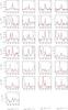 |
Fig. 1 Unblended transitions of EG from single-dish observations. The spectroscopic parameters (rest frequencies, quantum numbers, energies of the upper levels, and integrated intensities) from the LTE fit are listed in Table 3. For identification purposes, we have overplotted in red the LTE synthetic spectrum obtained with MADCUBAIJ assuming Tex = 50 K (see text). |
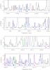 |
Fig. 2 Spectrum towards the peak of the continuum of the SMA compact data. We have overplotted the LTE synthetic spectrum of the different COMs obtained with MADCUBAIJ: EF (red), GA (light blue), MF (dark blue), DME (magenta), and ET (green). The colored circles indicate the unblended lines given in Table 4 and Tables B.2, B.4, B.6, and B.8. The physical parameters used are shown in Table C.2. |
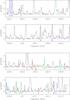 |
Fig. 2 continued. |
3. Line identification: Ethylene glycol and other COMs
A large frequency coverage is needed to robustly identify large COMs, especially in hot molecular cores where the density of lines in the spectra is high. To assure an identification at a 99%(99.8%) confidence level, at least 6(8) unblended lines are needed (Halfen et al. 2006). An additional condition is that all the detectable lines predicted by a local thermodynamic equilibrium (LTE) analysis that lie in the observed spectra must be revealed. Moreover, the relative intensities of the different transitions must be consistent with the LTE analysis, given the high-density environment of hot molecular cores. Furthermore, high spatial resolution data allow us to reduce the confusion limit of single-dish observations because different molecules may exhibit different spatial distributions.
The spectra of G31 exhibits a plethora of molecular lines of multiple species. Although a complete identification and analysis of all the detected lines is planned for a forthcoming paper (Rivilla et al., in prep.), we study here the emission of selected COMs, including EG. Our motivation is to compare their physical parameters and spatial distributions. These other complex species are: glycolaldehyde (GA), ethanol (C2H5OH, hereafter ET), methyl formate (CH3OCHO, hereafter MF), and dimethyl ether (CH3OCH3, hereafter DME). We also compare the spatial distribution of these COMs with that of methyl cyanide (CH3CN), a typical hot molecular tracer that has been studied in detail in Cesaroni et al. (2011).
We carried out the line identification of the COMs with MADCUBAIJ, which uses several molecular databases, including JPL3 and CDMS4. This software provides theoretical synthetic spectra of the different molecules under LTE conditions, taking into account the individual opacity of each line.
3.1. Single-dish data: GBT and IRAM 30 m
Our wide spectral coverage has allowed us to clearly identify multiple lines of all the different COMs. In Table 2 we summarize the molecules detected in each dataset. All the COMs have been detected in the different datasets, with the exception of GA and DME in the GBT data, because there are no bright lines of these species in the frequency range covered by the observations.
We confirm for the first time the detection of the lowest energy conformer (aGg’ conformer) of EG towards G31 (see details of the spectroscopy of EG in Appendix A). The single-dish data (GBT+IRAM 30 m) provide us with more than 30 unblended transitions of EG (see Fig. 1 and Table 3). These transitions cover an energy range of 5−114 K. We note that all the transitions predicted by the synthetic spectrum above 3σ are present in the observed spectra.
For identification purposes, we have overplotted in Fig. 1 the simulated LTE spectra provided by MADCUBAIJ, assuming a source size from the SMA maps (see Sect. 4.1). The relative intensities of the lines from 7 mm to 1.3 mm are well fitted with an excitation temperature of ~50 K. We note, however, that the LTE fit of multiwavelength transitions of EG underestimates the true temperature. The reason is explained in detail in Sect. 4.2.
We also detected multiple lines of the other COMs. In Appendix B we present tables with the unblended transitions detected for each species. In Figs. B.1 and B.2 we show selected lines at 3 mm and 7 mm detected with the IRAM 30 m and GBT telescopes, respectively, along with the LTE fits obtained with MADCUBAIJ (Table C.1).
3.2. Interferometric data: SMA
For the identification of lines we used the SMA datacube obtained with the compact interferometer configuration. Figure 4 shows the full SMA spectra (containing LSB and USB sidebands) towards the continuum peak. For identification purposes, we have overplotted the LTE synthetic spectra obtained with MADCUBAIJ of the different COMs, and have indicated with colored dots the lines least affected by blending. Several EG unblended lines are clearly identified (Fig. 4 and Table 4). The energy range covered by these transitions is 114−160 K. Additionally, the interferometric data allow us to map the spatial distribution of the EG emission. To study the spatial distribution of the emission we used the datacubes obtained by combining the data of both compact and very extended configurations, which provide a better spatial resolution (0.90″× 0.75″). Figure 3 confirms that the spatial distribution of different unblended EG lines is very similar. This spatial coherence supports the identification of EG.
Multiple lines of the other COMs have also been identified in the SMA data. Figure 4 shows the LTE spectra of the different COMs. The cleanest transitions of each molecule are listed in Appendix B (Tables B.2, B.4, B.6, and B.8).
4. Derivation of physical properties
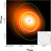 |
Fig. 3 Spatial distribution of EG transitions at 221.03880 GHz (white solid), 221.10032 GHz (white dashed), 230.57714 GHz (white dotted), and 230.830 GHZ (white dot-dashed), overplotted on the 1.3 mm continuum observed with the SMA (color scale). The black plus sign indicates the position of the peak of the 1.3 mm continuum. For comparison, we have also added the spatial distribution of the integrated emission of K = 0, 1, 2 CH3CN line (solid green line). All contours show the isocontour with 50% of the peak line intensity. The beam of the interferometer is shown in the lower right corner. |
4.1. Spatial distribution of EG and other COMs
The combined compact and very extended SMA observations have a nearly circular beam and a good uv coverage, thus allowing us to attain subarcsec resolution in all directions (0.90″× 0.75″; PA = 53°). Figure 4 shows the maps of the emission of different molecules obtained by integrating the emission under unblended lines. We defined the deconvolved beam size of the emitting regions as  , where θbeam is the half-power beam width of the interferometer and
  is the diameter of the circle whose area A equals that enclosed inside the contour level corresponding to 50% of the line peak.
The EG emission has a diameter of 0.7″, and peaks towards the position of the continuum (Fig. 4), similarly to that of GA and the vibrationally excited CH3CN v8 = 1. The EG emission is clearly smaller than the emission of other COMs like the ground vibrational level of CH3CN, ET and MF (Fig. 4 and Table 5). This is also observed in the Orion Hot Core, where EG is more compact than MF and ET (Brouillet et al. 2015).
The EG morphology differs from the “8-shaped” structure observed in ET, MF, or the ground state of CH3CN. Cesaroni et al. (2011) suggested that the “8-shaped” morphology is due to line opacity, which is higher at the center of the core and hence produces the observed dip. Since more complex molecules such as EG have lower abundances, they are expected to suffer less from line opacity effects and consequently allow us to trace gas located closer to the central protostar(s). This makes EG an excellent tracer of the physical properties and kinematics of the inner regions of hot cores, which can help us to understand massive star formation itself.
4.2. Importance of dust absorption in G31
In Sect. 3 we fit the 45−219 GHz single-dish spectra of EG using an LTE analysis with a temperature of 50 K using MADCUBAIJ. This temperature is significantly lower than that usually measured in hot cores, and in particular lower than the 164 K measured towards G31 by Beltrán et al. (2005) using CH CN and CH3CN v8 = 1. This discrepancy is striking, given that EG is tracing the innermost region of the core, as we have seen in the previous section, where a high temperature is expected. Since the low excitation transitions of EG (Eup = 5−45 K) have low frequencies (<113 GHz), and the higher excitation transitions (Eup = 79–114 K) have higher frequencies (>168 GHz), one may wonder if such a low temperature is due to the high-frequency (and high-energy) lines being somehow weakened with respect to the low-frequency (and low-energy) ones. Dust absorption provides us with a frequency-dependent mechanism of this type. In fact, dust opacity increases with frequency, τν ~ νβ, and hence may absorb at high frequency more effectively than at lower frequencies. This would result in an artificially low temperature when fitting with an LTE model.
To check whether this effect is at work in the G31 core, we studied in detail the emission of MF, which unlike EG has the advantage of multiple transitions that cover wide ranges of Eup at similar frequencies (and hence similarly affected by dust absorption). In the upper panel of Fig. 5 we present the rotational diagram of MF (which assumes optically thin emission; see, e.g., Goldsmith & Langer 1999) obtained from unblended MF transitions detected with single-dish data. The values shown on the y-axis have been corrected for beam dilution, using the size derived for MF of 1.7″ from the SMA maps (Table 5). We obtained a rotational temperature of ~75 K when considering all the MF transitions, similar to the low temperature found using EG, and again lower than that expected in this hot core.
We repeated the analysis distinguishing between three different frequency ranges. The temperatures obtained when fitting transitions separately at similar frequencies are higher (150−200 K, with an average value of ~170 K), in much better agreement with the value of 164 K derived by Beltrán et al. (2005). The upper panel of Fig. 5 confirms that transitions at higher frequencies are systematically shifted to lower values on the y-axis of the rotational diagram. We interpret this result as an indication of dust opacity in G31: the line photons at high frequencies are more absorbed by dust grains than those at lower frequencies, which decreases the corresponding line intensities.
We note that the shift in the y-axis of the rotational diagram between transitions in different frequency ranges cannot be due to different beam-dilutions at different frequencies. Even in the extreme case of extended emission filling the beam at all frequencies, the shift is still present (middle panel of Fig. 5). However, this is not the case. We know that both EG and MF emissions are not that extended because our high angular resolution interferometric maps show compact sizes of 0.7″ and 1.7″, respectively.
We suggest that the dust opacity is affecting the observed molecular line intensities. This effect is expected to be particularly important towards the innermost region of the core, where EG is detected. To support this interpretation, we studied whether the physical properties of G31 can indeed produce the dust absorption needed to explain the observed line intensities at different frequencies.
We derived the excitation temperature of MF considering only 3 mm transitions, which are the least affected by dust absorption. We selected transitions that cover a wide range of energy levels (20−200 K), which allows us to constrain the excitation temperature, and with similar frequencies (in the range 83−88 GHz) so that the effect of dust absorption is nearly the same. We obtained a value of Tex = 163 K, very similar to that derived by Beltrán et al. (2005).
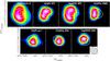 |
Fig. 4 Integrated emission maps of different COMs towards G31. All the maps have been obtained with the combination of the very extended and compact SMA data. The color scale in each panel spans from 30% to 100% of the line intensity peak. The frequencies (and upper energies) of the lines are: 220.747 GHz (69 K), 220.743 GHz (76 K), and 220.730 GHz (97 K) for CH3CN; 230.991 GHz (85 K) for ET; 229.405 GHz (111 K) and 229.420 (111 K) for MF; 230.234 (148 K) for DME; 221.228 GHz (698 K) for CH3CN v8 = 1; 221.100 (137 K) for EG; and 230.898 (131 K) for GA. The black solid line indicates the isocontour with 50% of the peak line intensity. The two white contours correspond to 50% and 80% of the peak value of the 1.3 mm continuum. The white plus sign indicates the positions of the peak of the 1.3 mm continuum. The beam of the interferometer is shown in the lower right corner of the lower right panel. |
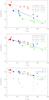 |
Fig. 5 Upper panel: rotational diagram of MF considering the beam dilution factor. The different colors indicate transitions in the different frequency ranges indicated by the labels. The black line is the best fit considering all transitions, while the colored lines are the best fits considering only the transitions in the same frequency range. Middle panel: same as upper panel, without considering beam dilution, i.e., assuming that the molecular emission completely fills the telescope beam. Lower panel: same as upper panel after correcting the line intensities for the dust opacity (solid circles) and without correction (open circles). |
It is possible to derive that the effect of dust opacity (τν) decreases the line intensities by a factor e−τν. Assuming a dust opacity index (τν ~ νβ) typical of massive star-forming cores of β = 1.5 (see, e.g., Palau et al. 2014), we then calculated the value of the opacity that would provide Tex = 163 K when fitting all the transitions at different frequencies, which is τ(220 GHz) = 2.6. The lower panel of Fig. 5 shows the rotational diagram of MF after correcting the line intensities for dust opacity.
It is possible to derive the hydrogen column density of the core from the obtained value of the opacity using the expression: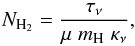 (1)where mH is the hydrogen mass, μ = 2.33 is the mean molecular mass per hydrogen atom, and κν is the absorption coefficient per unit density. For τ(220 GHz) = 2.6, assuming κ220GHz = 0.005 cm-2 g-1 and a gas-to-dust ratio of 100, the derived hydrogen column density is ~1.2 × 1026 cm-2. Using the deconvolved angular diameter of the continuum core of ~0.76″ (Cesaroni et al. 2011), this implies a total mass of ~2300 M⊙, which is consistent with the value of 1700 M⊙ obtained from the flux continuum emission by Cesaroni et al. (2011). The continuum flux density can be derived with the expression:
 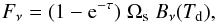 (2)where Ωs is the beam solid angle covered by the source, and B(Td) is the Planck function. Using
  /4 ln2, where θc is the deconvolved angular diameter of the continuum core (~0.76″, from Cesaroni et al. 2011) and assuming τ(220 GHz) = 2.6 and Td = 163 K, we obtain a continuum flux density of 3.8 Jy, consistent with the observed value (4.6 Jy, Cesaroni et al. 2011). Therefore, this confirms our interpretation that dust absorption is affecting the line intensities in G31. Obviously, the effect of dust absorption is expected to be important only if the level of clumpiness of the dense core is very low, i.e., if the dusty core is not fragmented into smaller condensations. Interestingly, recent high angular resolution (~0.2″) ALMA observations confirm that there is no hint of fragmentation in the continuum maps of G31 (Cesaroni, priv. comm.).
In summary, a LTE analysis of multifrequency transitions without considering the dust absorption underestimates the excitation temperatures, explaining the intriguingly low temperature of 50 K derived for EG when fitting multiwavelength transitions. In the next section we explain how to derive reliable values of the excitation temperatures and hence of molecular column densities.
4.3. Molecular column densities
Keeping the effect of dust absorption in mind, to obtain the physical parameters of the different COMs, we restricted our analysis to the IRAM 30 m 3 mm transitions, the least affected by the dust opacity. We used MADCUBAIJ to fit the observed 3 mm spectra with the LTE model5. MADCUBAIJ considers five different parameters to create the simulated LTE spectra: column density of the molecule (N), excitation temperature (Tex), linewidth (Δv), velocity (v), and source size (θs). The procedure used to derive the main physical parameters is the following:
i) we fix the velocity of the emission and the linewidth to the values obtained from Gaussian fits of unblended lines; ii) we fix the gas temperature to the value estimated using the 3 mm transition of MF (163 K), which is a good temperature tracer (Favre et al. 2011); iii) to obtain the source-average column density Ns, we fix the size of the molecular emission to the value obtained from the integrated maps of clean lines detected with the SMA, and apply the beam dilution factor accordingly; instead we do not apply the beam dilution factor to derive the beam-averaged column density Nb; iv) leaving N as free parameter, we use the AUTOFIT tool of MADCUBAIJ to find the value that fits the unblended molecular transitions of each COM better.
The results for the different molecular species are summarized in Table 6. To account for the dust absorption discussed above, the values for the column densities have been corrected by a factor eτ(3 mm) ~ 2, where τ(3 mm) has been derived assuming the derived value of τ(220 GHz) = 2.6 and β = 1.5.
The main source of uncertainty in the estimated column densities arises from the assumption of the LTE approximation using a single temperature. However, even in the extreme case that the temperature varies by a factor of 2, the variation in the derived column densities would be less than a factor of 2. We therefore consider that the uncertainty in the estimated column densities is less than a factor of 2.
All the molecules have velocities very close to the source systemic velocity, ~97 km s-1, and linewidths (FWHM) ~5 km s-1, typical of hot molecular cores. The derived source-averaged molecular abundances with respect to molecular hydrogen are in the range ~(0.3−8) × 10-8.
5. Comparison with other interstellar sources
5.1. Comparison with other star-forming regions
We compared the relative molecular abundances obtained in G31 with those already reported in other star-forming regions: the massive star-forming regions in Orion KL (Brouillet et al. 2015), W51e2, and G34.3+0.2 (Lykke et al. 2015); the intermediate-mass star-forming region NGC 7129 FIRS2 (Fuente et al. 2014); and the low-mass protostars IRAS 16293-2422 (Jørgensen et al. 2012), NGC 1333 IRAS 2A (Maury et al. 2014; Coutens et al. 2015; Taquet et al. 2015), and NGC 133 IRAS 4A (Taquet et al. 2015). The different relative molecular abundances are given in Table 7. The uncertainty of the abundance ratios can be estimated by considering propagation of the uncertainty of the column densities of each molecule. We expect then that the uncertainty of relative molecular ratios is less than a factor of 3. In Fig. 6 we show the behavior of the different abundance ratios with respect to the luminosity of the sources.
Table 7 shows that EG is always more abundant than GA in all star-forming regions. This has also been noted by Requena-Torres et al. (2008) in the Galactic Center, where saturated species, such as EG, are always more abundant than unsaturated species, such as GA (see Table 7); and in star-forming regions (e.g. Ikeda et al. 2001; Hollis et al. 2002; Bisschop et al. 2007) Therefore, there is evidence that chemistry favors saturated versus unsaturated species. Requena-Torres et al. (2008) suggested that the double bond C=O (present in the unsaturated species, e.g. GA) can be easily broken.
In star-forming regions, the [EG/GA] ratio changes with luminosity, spanning from 1 to >15. The lower limits of the higher luminosity sources (hot cores) suggest that the [EG/GA] ratio increases with luminosity.
The [DME/MF] and [EG/ET] ratios are nearly constant with luminosity, with values of the order of ~1 and ~0.1, respectively. The [GA/MF] and [ET/DME] ratios clearly decrease with increasing luminosity. In Sect. 6 we discuss how these results can help us to understand the formation of EG and other COMs.
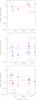 |
Fig. 6 Relative abundances of pairs of COMs with respect to the luminosity of the star-forming regions. The conservative uncertainty of the relative abundances correspond to a factor of 3 (see text). The triangles in the upper(lower) panels are lower(upper) limits. The solid horizontal lines correspond to the relative abundance value found in the comet Lovejoy, from Biver et al. (2015). |
Physical parameters obtained from the 3 mm IRAM 30 m data for the different molecules.
5.2. Comparison with quiescent clouds and comets
The formation of stars and planets undergoes different evolutionary stages: i) cold and dense prestellar cores are able to collapse, triggering star formation; ii) the gravitational energy is converted into thermal energy and radiation, and the forming star warms up the dense neighboring envelope; and iii) the envelope dissipates and a circumstellar disk remains, where eventually planets and other bodies such as comets are formed. We investigate here whether there is any hint of a chemical trend between different evolutionary phases of the ISM: quiescent clouds, star-forming regions and comets. To this end we have also included in Table 7 the relative abundance ratios towards quiescent clouds located in the Galactic Center, G-002, G-001, G+0.693 (Requena-Torres et al. 2008), and the comets Hale-Bopp (Crovisier et al. 2004), Lemmon (Biver et al. 2014), Lovejoy (Biver et al. 2015), and 67P/Churyumov-Gerasimenko (Goesmann et al. 2015). In Fig. 7 we compare different molecular abundance ratios between these three groups of sources (i.e., comets, star-forming regions, and quiescent clouds).
We find that for all kind of sources [EG/GA] > [EG/ET] > [GA/MF]. This suggests that the relative abundances of different COMs, despite the observed large dispersions, share a general trend in interstellar sources at different evolutionary stages. This might mean that the chemistry at different stages of star formation is not significantly different, and there is a chemical thread across the entire star formation process. However, the low number of sources with positive detections of these COMs is still low, and prevents a statistically significant conclusion.
Relative abundances of COMs in comets, star-forming regions and Galactic Center quiescent clouds.
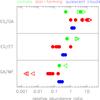 |
Fig. 7 Comparison of different ratios of molecular abundances of COMs between comets, star-forming regions, and quiescent clouds. The color circles indicate measured ratios, while right and left-oriented triangles denote lower and upper limits. |
6. Discussion: formation of ethylene glycol and other COMs in star-forming regions
We detected 30 unblended transitions of EG with single-dish observations and 5 unblended transitions with interferometric observations. We note that the best detection so far of EG (in SgrB2 N, the prototypical interstellar source for the search of large COMs) relies on the detection of only ~13 unblended lines (Belloche et al. 2013), despite the much wider spectral coverage of these observations. This clearly shows that although the extreme conditions of the Galactic Center create a unique chemically rich environment, paradoxically the presence of so many molecules produces blending problems that make it difficult to identify molecules with faint emission. Moreover, in SgrB2 N multiple velocity components and strong absorption also complicate a correct identification of the lines. Therefore, sources with relatively simple structure and kinematics, but also chemically rich, such as G31, are a good alternative to carry out astrochemical studies. Furthermore, our work proves that single-dish observations are suitable for the detection of large COMs in hot molecular cores, despite the beam dilution. Obviously, interferometric observations at high resolution are also needed to measure the size of the emitting regions and hence obtain proper values of the molecular abundances.
The formation of COMs is still an open debate in astrophysics. Theoretical chemical models based only on gas-phase reactions have failed by orders of magnitude to reproduce the observed abundances of COMs (e.g., Geppert et al. 2006). Moreover, in the particular case of EG and GA there are no known gas-phase reactions to form GA or EG (see the chemical databases KIDA6 and UMIST7; and also Woods et al. 2012). For this reason, chemistry on the surface of dust grains has been invoked to form COMs (e.g., Garrod et al. 2008), which would be subsequently desorbed as a result of heating from the central protostar or from shocks, enriching the molecular environment. However, Balucani et al. (2015) have recently pointed out that some gas-phase reactions are feasible, and that gas-phase chemistry should also be considered as an alternative to form COMs.
Based on the derived molecular abundances in G31 and other star-forming regions, we discuss in this section how observations can give us clues about the formation of COMs.
We have found that the [EG/GA] ratio seems to increase with the luminosity of the source, from the low values of ~1 found towards the low-mass protostar IRAS 16293-2422 (Jørgensen et al. 2012; and Jorgensen et al., in prep.) to the higher value of ~10 towards the hot core G31 and the lower limits of the hot cores in Orion, W51e2, and G34.3+0.2, which are as high as >15. We have also found that while the [DME/MF] and [EG/ET] are nearly constant with luminosity, the ratios between the pair of isomers [GA/MF] and [ET/DME] decrease with luminosity. In the following sections we propose different mechanisms that are able to explain these observational trends, and that give us hints about the formation of COMs in star-forming regions: i) different chemical formation routes; ii) different warm-up timescales; iii) different initial gas compositions of the dust grains; iv) different hydrogen densities of the sources; v) different formation/destruction efficiency in the gas phase.
6.1. Chemical link
Table 8 shows different chemical routes proposed in the literature to form the COMs studied in this work: EG, GA, MF, DME, and ET. These chemical routes rely on theoretical chemical models (Bennett & Kaiser 2007; Garrod et al. 2008; Woods et al. 2013; Balucani et al. 2015) and laboratory experiments (Fedoseev et al. 2015; Butscher et al. 2015).
Chemical routes proposed in the literature for the formation of various COMs studied in this work.
If two molecular species are chemically linked, i.e., if they have a common precursor and/or one is formed from the other, their relative abundance ratio should be nearly constant regardless of the luminosity of the source. This occurs, for instance, in the [DME/MF] ratio (middle panel of Fig. 6), which is ~1 for all star-forming regions. This chemical link suggested by the observations is indeed predicted by theoretical models. Garrod et al. (2008) proposed that both MF and DME form from the common precursor methoxy (CH3O) by surface chemistry on dust grains (route 5 and 7 in Table 8, respectively). In addition, Balucani et al. (2015) have proposed a new gas-phase route that can efficiently contribute to the formation of MF directly from DME (route 6 in Table 8). In any case, it seems that MF and DME are chemically linked, in agreement with the observed constant abundance ratio.
Likewise, if EG were formed by sequential hydrogenation of GA as suggested by the route 1, a relatively constant [EG/GA] ratio would be expected. Instead, the values of the [EG/GA] ratio differ between sources by more than an order of magnitude, from 1 to >15 (upper panel of Fig. 6). This suggests that EG and GA are not directly linked.
Therefore, it seems more plausible that EG is formed by the combination of two CH2OH radicals (route 2 in Table 8). Although Walsh et al. (2014) have raised some doubts about the efficiency of this process owing to the low mobility produced by the OH-bonds, the recent experimental work by Butscher et al. (2015) has shown that this mechanism seems to be a very efficient pathway to form EG.
The large variation of the [EG/GA] ratio suggests not only that GA is not the direct precursor of EG, but also that they do not share a common precursor. Since we favor the formation of EG by the combination of two CH2OH radicals (route 2), this would imply that CH2OH is not a precursor of GA, and route 4 can be ruled out. Then, the chemical pathway based on the dimerization of HCO (route 3) proposed by Woods et al. (2013) appears to be the most plausible scenario. This route has also been recently supported by the laboratory experiments of Fedoseev et al. (2015).
The nearly constant behavior of the [EG/ET] ratio with luminosity (middle panel of Fig. 6) suggests that these two species might be chemically linked. Indeed, this agrees with the chemical model proposed by Garrod et al. (2008), which produces EG and ET from the common precursor CH2OH (routes 2 and 8, respectively).
In conclusion, the observed abundance ratios can all be justified by routes 2 (for EG), route 3 (for GA), routes 5 and/or 6 (for MF), route 7 (for DME), and route 8 (for ET), while routes 1 and 4 are excluded.
6.2. Timescales
The different warm-up timescales associated with objects of different luminosities (hot cores and hot corinos) are expected to affect the chemistry. We discuss here whether this effect is able to explain the behavior of the relative molecular abundances with luminosity observed in Fig. 6. According to Garrod et al. (2008), the [EG/GA] and [ET/DME] ratios are higher at longer warm-up timescales, while the ratio [GA/MF] decreases with the timescale. Assuming that the warm phase in hot cores is longer than in hot corinos, as indicated by the chemical models by Awad et al. (2014), then the heating timescale would be proportional to the luminosity. Hence, the timescale effect could contribute to explain the observed trend of [ET/DME], but not those of [EG/GA] and [GA/MF].
6.3. Chemical composition of dust grains
A possible explanation for the different [EG/GA] ratios is different chemical compositions of the dust grains in different star-forming regions. The experiments of Öberg et al. (2009) indicate that different initial compositions of the ices could produce very different values of the [EG/GA] ratio: pure CH3OH ices produce a ratio >10, while ices with a composition CH3OH:CO 1:10 produce a ratio <0.25. If this were the explanation for the different [EG/GA] ratios, it would imply that the initial composition of grains is different for low- and high-mass star-forming regions.
6.4. Atomic hydrogen density
The experiments and chemical modeling by Fedoseev et al. (2015) show that different initial atomic H densities provide different [EG/GA] ratios. Coutens et al. (2015) argue that the density could explain the difference observed towards IRAS 16293-2422 and NGC 1333 IRAS 2A, with [EG/GA] ratios of 1 and 5, respectively. They suggest that the lower H2 density of IRAS 2A would lead to a higher atomic H density and then to a higher [EG/GA] ratio, as observed. However, this scenario does not apply to G31, which is denser and exhibits an even higher [EG/GA] ratio. Therefore, we believe that atomic hydrogen density cannot explain the observed behavior of the [EG/GA] ratio.
6.5. Formation and destruction on gas phase
So far we have assumed in our discussion that COMs are mainly formed by surface chemistry on dust grains and subsequently desorbed into the gas phase. However, the situation can be more complex if we also consider gas phase formation routes. Recently, Balucani et al. (2015) have suggested that some gas reactions may be important for the formation of MF in cold environments. If this were also the case for GA and EG, for which no efficient gas phase reactions are available to date (see Woods et al. 2012), the interpretation of the observational results should be revisited. More theoretical work is needed to make this hypothesis plausible.
Finally, another possible cause for the variation of the [EG/GA] ratio could be different destruction mechanisms in the gas phase. Hudson et al. (2005) show that GA is more sensitive to irradiation than EG, which may explain its lower abundance in luminous sources. Higher levels of irradiation by the higher luminosity sources would produce an increase in the [EG/GA] ratio with luminosity, as observed. However, the destruction pathways of these COMs have not yet been explored by the theoretical models and laboratory experiments.
7. Summary and conclusions
We have reported for the first time the detection of the aGg’ conformer of the ten-atoms organic molecule ethylene glycol, (CH2OH)2, towards the hot molecular core G31.41+0.31. This and previous detections of COMs (e.g., CH2OHCHO) confirm that G31.41+0.31 is an excellent laboratory for studying the astrochemistry related with the building blocks of primordial life. We have detected multiple unblended transitions of (CH2OH)2 with single-dish and interferometric observations. Our SMA interferometric maps show that the (CH2OH)2 emission is very compact, with a diameter of 0.7″, peaking towards the maximum of the continuum. This morphology is similar to that observed in vibrationally excited CH3CN or CH2OHCHO, and differs from that observed in other more abundant COMs such as the ground state of CH3CN or CH3OCHO, which exhibit a dip in the central region. We propose that this difference is likely due to line opacity. Lower abundance molecules such as (CH2OH)2 and CH2OHCHO are expectd to be more optically thin and allow us to trace the gas closest to the forming protostar(s).
Our detailed LTE analysis of (CH2OH)2 and CH3OCHO towards G31.41+0.31 suggests that dust opacity plays an important role in the line intensities. We have found evidence that high-frequency transitions are more efficiently absorbed than low-frequency transitions owing to higher dust opacity. This effect should be taken into account to derive a correct value of the excitation temperature and column density of molecules in dense hot molecular cores. We have derived the molecular abundances of several COMs towards G31.41+0.31 (CH2OHCHO, (CH2OH)2, C2H5OH, and CH3OCH3), finding abundances with respect to molecular hydrogen in the range (0.3−8) × 10-8 .
Observations in different star-forming regions indicate that the ratio (CH2OH)2/CH2OHCHO spans from 1 to >15. We have found evidence of an increase in the ratio with the luminosity of the source. We have discussed different possible explanations for this trend, concluding that the most likely scenario is that both species are formed through different chemical routes that are not directly linked. We cannot exclude, however, a contribution of different formation and destruction efficiencies in the gas phase of both species, but more laboratory work and theoretical chemical models are needed to better constrain this hypothesis.
We have discussed the molecular abundance ratios of COMs in different star-forming regions in the context of the different chemical routes proposed for their formation. We conclude that observations favor the formation of (CH2OH)2 by the combination of two CH2OH radicals on dust grains, in agreement with the models of Bennett & Kaiser (2007) and Garrod et al. (2008), and the laboratory experiments by Butscher et al. (2015). The most likely formation route of CH2OHCHO is via solid-phase dimerization of the formyl radical HCO, a mechanism proposed by Woods et al. (2013) and supported by the laboratory experiments of Fedoseev et al. (2015). The observational data also suggests that CH3OCHO and CH3OCH3 are chemically linked, which may mean that both share a common precursor, CH3O, as proposed by Garrod et al. (2008), or that the former is directly formed from the latter through viable gas-phase reactions, as suggested by Balucani et al. (2015). Similarly, EG and ET might share the common precursor CH2OH.
The behavior of the abundance ratio C2H5OH/CH3OCH3 with luminosity may be explained by the different warm-up timescales in hot cores and hot corinos.
Madrid Data Cube Analysis on ImageJ is a software developed by the Center of Astrobiology (Madrid, INTA-CSIC) to visualize and analyze single spectra and datacubes (Martín et al., in prep.).
The Submillimeter Array is a joint project between the Smithsonian Astrophysical Observatory and the Academia Sinica Institute of Astronomy and Astrophysics, and is funded by the Smithsonian Institution and the Academia Sinica (Ho et al. 2004).
The lowercase letters a and g correspond to rotation at the CO bond where clockwise/counterclockwise rotation is indicated by a positive/negative diedral angle and the symbols g/g’. The rotational directions are determined by looking along the C–C and C–O axes from the first to the second atom.
Acknowledgments
This work was partly supported by the Italian Ministero dell’Istruzione, Univertitá e Ricerca through the grant Progetti Premiali 2012 – iALMA.
References
- Awad, Z., Viti, S., Bayet, E., & Caselli, P. 2014, MNRAS, 443, 275 [NASA ADS] [CrossRef] [Google Scholar]
- Balucani, N., Ceccarelli, C., & Taquet, V. 2015, MNRAS, 449, L16 [Google Scholar]
- Belloche, A., Müller, H. S. P., Menten, K. M., Schilke, P., & Comito, C. 2013, A&A, 559, A47 [NASA ADS] [CrossRef] [EDP Sciences] [Google Scholar]
- Beltrán, M. T., & de Wit, W. J. 2016, A&ARv, 24, 6 [NASA ADS] [CrossRef] [Google Scholar]
- Beltrán, M. T., Cesaroni, R., Neri, R., et al. 2005, A&A, 435, 901 [NASA ADS] [CrossRef] [EDP Sciences] [Google Scholar]
- Beltrán, M. T., Codella, C., Viti, S., Neri, R., & Cesaroni, R. 2009, ApJ, 690, L93 [NASA ADS] [CrossRef] [Google Scholar]
- Bennett, C. J., & Kaiser, R. I. 2007, ApJ, 661, 899 [NASA ADS] [CrossRef] [Google Scholar]
- Bisschop, S. E., Jørgensen, J. K., van Dishoeck, E. F., & de Wachter, E. B. M. 2007, A&A, 465, 913 [NASA ADS] [CrossRef] [EDP Sciences] [Google Scholar]
- Biver, N., Bockelée-Morvan, D., Debout, V., et al. 2014, A&A, 566, L5 [Google Scholar]
- Biver, N., Bockelée-Morvan, D., Moreno, R., & Crovisier, J. A. A. 2015, Sci. Adv., 1, e1500863 [Google Scholar]
- Brouillet, N., Despois, D., Lu, X.-H., et al. 2015, A&A, 576, A129 [NASA ADS] [CrossRef] [EDP Sciences] [Google Scholar]
- Butscher, T., Duvernay, F., Theule, P., et al. 2015, MNRAS, 453, 1587 [NASA ADS] [CrossRef] [Google Scholar]
- Cesaroni, R., Beltrán, M. T., Zhang, Q., Beuther, H., & Fallscheer, C. 2011, A&A, 533, A73 [NASA ADS] [CrossRef] [EDP Sciences] [Google Scholar]
- Charnley, S. B., & Rodgers, S. D. 2005, in Astrochemistry: Recent Successes and Current Challenges, eds. D. C. Lis, G. A. Blake, & E. Herbst, 237 [Google Scholar]
- Christen, D., & Müller, H. S. P. 2003, Phys. Chem. Chem. Phys., 5, 3600 [Google Scholar]
- Christen, D., Coudert, L. H., Suenram, R., & Lovas, F. J. 1995, J. Mol. Spectr., 172, 57 [NASA ADS] [CrossRef] [Google Scholar]
- Christen, D., Coudert, L. H., Larsson, J. A., & Cremer, D. 2001, J. Mol. Spectr., 205, 185 [NASA ADS] [CrossRef] [Google Scholar]
- Churchwell, E., Walmsley, C. M., & Cesaroni, R. 1990, A&AS, 83, 119 [NASA ADS] [Google Scholar]
- Collins, P., & Ferrier, R. 1995, Monosaccharides, Their Chemistry and Their Roles in Natural Products (Wiley) [Google Scholar]
- Cooper, G., Kimmich, N., Belisle, W., et al. 2001, Nature, 414, 879 [NASA ADS] [CrossRef] [PubMed] [Google Scholar]
- Coutens, A., Persson, M. V., Jørgensen, J. K., Wampfler, S. F., & Lykke, J. M. 2015, A&A, 576, A5 [NASA ADS] [CrossRef] [EDP Sciences] [Google Scholar]
- Crovisier, J., Bockelée-Morvan, D., Biver, N., et al. 2004, A&A, 418, L35 [NASA ADS] [CrossRef] [EDP Sciences] [Google Scholar]
- Favre, C., Despois, D., Brouillet, N., et al. 2011, A&A, 532, A32 [NASA ADS] [CrossRef] [EDP Sciences] [Google Scholar]
- Fedoseev, G., Cuppen, H. M., Ioppolo, S., Lamberts, T., & Linnartz, H. 2015, MNRAS, 448, 1288 [NASA ADS] [CrossRef] [Google Scholar]
- Fontani, F., Pascucci, I., Caselli, P., et al. 2007, A&A, 470, 639 [NASA ADS] [CrossRef] [EDP Sciences] [Google Scholar]
- Fuente, A., Cernicharo, J., Caselli, P., et al. 2014, A&A, 568, A65 [NASA ADS] [CrossRef] [EDP Sciences] [Google Scholar]
- Garrod, R. T., Weaver, S. L. W., & Herbst, E. 2008, ApJ, 682, 283 [NASA ADS] [CrossRef] [Google Scholar]
- Geppert, W. D., Hamberg, M., Thomas, R. D., et al. 2006, Faraday Discussions, 133, 177 [Google Scholar]
- Goesmann, F., Rosenbauer, H., Bredehöft, J. H., et al. 2015, Science, 349, 020689 [CrossRef] [Google Scholar]
- Goldsmith, P. F., & Langer, W. D. 1999, ApJ, 517, 209 [NASA ADS] [CrossRef] [Google Scholar]
- Halfen, D. T., Apponi, A. J., Woolf, N., Polt, R., & Ziurys, L. M. 2006, ApJ, 639, 237 [NASA ADS] [CrossRef] [Google Scholar]
- Ho, P. T. P., Moran, J. M., & Lo, K. Y., 2004, ApJ, 616, L1 [NASA ADS] [CrossRef] [Google Scholar]
- Hollis, J. M., Lovas, F. J., Jewell, P. R., & Coudert, L. H. 2002, ApJ, 571, L59 [NASA ADS] [CrossRef] [Google Scholar]
- Hudson, R. L., Moore, M. H., & Cook, A. M. 2005, Adv. Space Res., 36, 184 [NASA ADS] [CrossRef] [Google Scholar]
- Ikeda, M., Ohishi, M., Nummelin, A., et al. 2001, ApJ, 560, 792 [NASA ADS] [CrossRef] [Google Scholar]
- Isokoski, K., Bottinelli, S., & van Dishoeck, E. F. 2013, A&A, 554, A100 [NASA ADS] [CrossRef] [EDP Sciences] [Google Scholar]
- Jørgensen, J. K., Favre, C., Bisschop, S. E., et al. 2012, ApJ, 757, L4 [NASA ADS] [CrossRef] [Google Scholar]
- Krishnamurthy, R., Arrhenius, G., & Eschenmoser, A. 1999, Origins of Life and Evolution of the Biosphere, 29, 333 [NASA ADS] [CrossRef] [Google Scholar]
- Lykke, J. M., Favre, C., Bergin, E. A., & Jørgensen, J. K. 2015, A&A, 582, A64 [NASA ADS] [CrossRef] [EDP Sciences] [Google Scholar]
- Maury, A. J., Belloche, A., André, Ph., et al. 2014, A&A, 563, L2 [NASA ADS] [CrossRef] [EDP Sciences] [Google Scholar]
- Öberg, K. I., Garrod, R. T., van Dishoeck, E. F., & Linnartz, H. 2009, A&A, 504, 891 [NASA ADS] [CrossRef] [EDP Sciences] [Google Scholar]
- Palau, A., Estalella, R., Girart, J. M., et al. 2014, ApJ, 785, 42 [NASA ADS] [CrossRef] [Google Scholar]
- Requena-Torres, M. A., Martín-Pintado, J., Martín, S., & Morris, M. R. 2008, ApJ, 672, 352 [NASA ADS] [CrossRef] [Google Scholar]
- Rivilla, V. M., Fontani, F., Beltrán, M. T., et al. 2016, ApJ, 826, 161 [NASA ADS] [CrossRef] [Google Scholar]
- Sorrell, W. H. 2001, ApJ, 555, L129 [NASA ADS] [CrossRef] [Google Scholar]
- Taquet, V., López-Sepulcre, A., Ceccarelli, C., et al. 2015, ApJ, 804, 81 [NASA ADS] [CrossRef] [Google Scholar]
- Walsh, C., Millar, T. J., Nomura, H., et al. 2014, A&A, 563, A33 [NASA ADS] [CrossRef] [EDP Sciences] [Google Scholar]
- Weber, A. L. 1998, Origins of Life and Evolution of the Biosphere, 28, 259 [NASA ADS] [CrossRef] [Google Scholar]
- Woods, P. M., Kelly, G., Viti, S., et al. 2012, ApJ, 750, 19 [NASA ADS] [CrossRef] [Google Scholar]
- Woods, P. M., Slater, B., Raza, Z., et al. 2013, ApJ, 777, 90 [NASA ADS] [CrossRef] [Google Scholar]
Appendix A: Spectroscopy of ethylene glycol
Ethylene glycol is a triple rotor molecule. Torsions around its C−C bond and its two C−O bonds lead to ten different conformers, four forms with an anti (A) arrangement of the OH groups and six with a gauche (G) arrangement (Fig. 1 from Christen et al. 2001). Two of the G conformers are capable of establishing intramolecular hydrogen bonds, known as g’Ga and g’Gg8, which are expected to be energetically favorable in the gas phase. The aGg’ conformer of EG is the lowest energy state conformer. The torsion of both hydroxyl groups (OH) around the two CO bonds produces a tunneling splitting. This translates into two sublevels, v = 0 and v = 1, separated by ~7 GHz. Within each tunneling sublevel, the different rotational energy levels are characterized by three quantum numbers, J, Ka, Kc. To label the different energy levels we use in this paper the following notation JKa,Kc, v = 0 or 1. The transitions occur for changes from a rotational level in the v = 1 state to a rotational level in the v = 0 state, or viceversa. Figure 2 of Christen et al. (1995) shows a fraction of the energy
level diagram of the g’Ga conformer of EG. In our analysis we used the experimental spectrum of the aGg’ conformer obtained by Christen et al. (1995) and Christen & Müller (2003).
Appendix B: Identified unblended transitions of COMs
We present in this appendix several tables with the unblended transitions of the different COMs found in the single-dish and interferometric data: ET (Tables B.1 and B.2), MF (Tables B.3 and B.4), GA (Tables B.5 and B.6), and DME (Tables B.7 and B.8).
In Fig. B.1 we also present some selected IRAM 30 m spectra at 3 mm of MF, ET, DME, and GA. We have overplotted in red the LTE fit using MADCUBAIJ with the physical parameters shown in Table 6.
In Fig. B.2 we present the unblended transitions of the COMs detected with the GBT telescope.
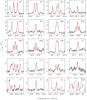 |
Fig. B.1 Selected transitions at 3 mm of COMs detected towards the G31.41+0.31 hot molecular core with the IRAM 30 m telescope: methyl formate (MF), dimethyl ether (DME), ethanol (ET) and glycolaldehyde (GA). Overplotted in red are the LTE synthetic spectra obtained with MADCUBAIJ using the physical parameters given in Table 6. |
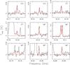 |
Fig. B.2 Unblended transitions of the COMs detected towards the G31.41+0.31 hot molecular core with the GBT telescope: ethylene glycol (EG), ethanol (ET) and methyl formate (MF). Overplotted in red are the LTE synthetic spectra obtained with MADCUBAIJ using the physical parameters given in Table C.1. |
Unblended transitions of ET identified in the single-dish spectra (GBT and IRAM 30 m) towards G31.
Unblended transitions of ET identified in the interferometric SMA spectra towards G31.
Unblended transitions (i.e. non blended with other molecular species) of MF identified in the single-dish spectra (GBT and IRAM 30 m) towards G31.
Unblended transitions (i.e. non blended with other molecular species) of MF identified in the interferometric SMA spectra towards G31.
Unblended transitions (i.e. non blended with other molecular species) of GA identified in the single IRAM 30 m single-dish spectra towards G31.
Unblended transition of GA identified in the interferometric SMA spectra towards G31.
Unblended transitions of DME identified in the IRAM 30 m single-dish spectra towards G31.
Unblended transitions (i.e. non blended with other molecular species) of DME identified in the interferometric SMA spectra towards G31.
Appendix C: MADCUBAIJ LTE fits of the GBTand SMA data
In this appendix we present the physical parameters used to model with MADCUBAIJ the transitions of the different COMs in the GBT and SMA spectra (Figs. B.2 and 2, respectively). The procedure used is: i) we fix the velocity of the emission and the linewidth to the values obtained from Gaussian fits of unblended lines; ii) to obtain the source-average column density Ns, we fix the size of the molecular emission to the value obtained from the integrated maps of unblended lines detected with the SMA, and apply the beam dilution factor accordingly; while we do not apply the beam dilution factor to derive the beam-average column density Nb; iii) leaving N and Tex as free parameters, we use the AUTOFIT tool of MADCUBAIJ to find the pair of values that fits the unblended molecular transitions of each COM better.
MADCUBAIJ best fits of the COMs detected in the GBT spectra.
MADCUBAIJ best fits of the SMA compact spectra towards the peak of the continuum for the different molecules.
All Tables
Summary of the detections of the different COMs in the different telescope datasets.
Clean transitions (i.e., not blended with other molecular species) of EG identified in the single-dish spectra (GBT and IRAM 30 m) towards G31.
Clean transitions (i.e., not blended with other molecular species) of EG identified in the interferometric SMA spectra towards G31.
Physical parameters obtained from the 3 mm IRAM 30 m data for the different molecules.
Relative abundances of COMs in comets, star-forming regions and Galactic Center quiescent clouds.
Chemical routes proposed in the literature for the formation of various COMs studied in this work.
Unblended transitions of ET identified in the single-dish spectra (GBT and IRAM 30 m) towards G31.
Unblended transitions of ET identified in the interferometric SMA spectra towards G31.
Unblended transitions (i.e. non blended with other molecular species) of MF identified in the single-dish spectra (GBT and IRAM 30 m) towards G31.
Unblended transitions (i.e. non blended with other molecular species) of MF identified in the interferometric SMA spectra towards G31.
Unblended transitions (i.e. non blended with other molecular species) of GA identified in the single IRAM 30 m single-dish spectra towards G31.
Unblended transition of GA identified in the interferometric SMA spectra towards G31.
Unblended transitions of DME identified in the IRAM 30 m single-dish spectra towards G31.
Unblended transitions (i.e. non blended with other molecular species) of DME identified in the interferometric SMA spectra towards G31.
MADCUBAIJ best fits of the SMA compact spectra towards the peak of the continuum for the different molecules.
All Figures
|
Fig. 1 Unblended transitions of EG from single-dish observations. The spectroscopic parameters (rest frequencies, quantum numbers, energies of the upper levels, and integrated intensities) from the LTE fit are listed in Table 3. For identification purposes, we have overplotted in red the LTE synthetic spectrum obtained with MADCUBAIJ assuming Tex = 50 K (see text). |
| In the text | |
|
Fig. 2 Spectrum towards the peak of the continuum of the SMA compact data. We have overplotted the LTE synthetic spectrum of the different COMs obtained with MADCUBAIJ: EF (red), GA (light blue), MF (dark blue), DME (magenta), and ET (green). The colored circles indicate the unblended lines given in Table 4 and Tables B.2, B.4, B.6, and B.8. The physical parameters used are shown in Table C.2. |
| In the text | |
|
Fig. 2 continued. |
| In the text | |
|
Fig. 3 Spatial distribution of EG transitions at 221.03880 GHz (white solid), 221.10032 GHz (white dashed), 230.57714 GHz (white dotted), and 230.830 GHZ (white dot-dashed), overplotted on the 1.3 mm continuum observed with the SMA (color scale). The black plus sign indicates the position of the peak of the 1.3 mm continuum. For comparison, we have also added the spatial distribution of the integrated emission of K = 0, 1, 2 CH3CN line (solid green line). All contours show the isocontour with 50% of the peak line intensity. The beam of the interferometer is shown in the lower right corner. |
| In the text | |
|
Fig. 4 Integrated emission maps of different COMs towards G31. All the maps have been obtained with the combination of the very extended and compact SMA data. The color scale in each panel spans from 30% to 100% of the line intensity peak. The frequencies (and upper energies) of the lines are: 220.747 GHz (69 K), 220.743 GHz (76 K), and 220.730 GHz (97 K) for CH3CN; 230.991 GHz (85 K) for ET; 229.405 GHz (111 K) and 229.420 (111 K) for MF; 230.234 (148 K) for DME; 221.228 GHz (698 K) for CH3CN v8 = 1; 221.100 (137 K) for EG; and 230.898 (131 K) for GA. The black solid line indicates the isocontour with 50% of the peak line intensity. The two white contours correspond to 50% and 80% of the peak value of the 1.3 mm continuum. The white plus sign indicates the positions of the peak of the 1.3 mm continuum. The beam of the interferometer is shown in the lower right corner of the lower right panel. |
| In the text | |
|
Fig. 5 Upper panel: rotational diagram of MF considering the beam dilution factor. The different colors indicate transitions in the different frequency ranges indicated by the labels. The black line is the best fit considering all transitions, while the colored lines are the best fits considering only the transitions in the same frequency range. Middle panel: same as upper panel, without considering beam dilution, i.e., assuming that the molecular emission completely fills the telescope beam. Lower panel: same as upper panel after correcting the line intensities for the dust opacity (solid circles) and without correction (open circles). |
| In the text | |
|
Fig. 6 Relative abundances of pairs of COMs with respect to the luminosity of the star-forming regions. The conservative uncertainty of the relative abundances correspond to a factor of 3 (see text). The triangles in the upper(lower) panels are lower(upper) limits. The solid horizontal lines correspond to the relative abundance value found in the comet Lovejoy, from Biver et al. (2015). |
| In the text | |
|
Fig. 7 Comparison of different ratios of molecular abundances of COMs between comets, star-forming regions, and quiescent clouds. The color circles indicate measured ratios, while right and left-oriented triangles denote lower and upper limits. |
| In the text | |
|
Fig. B.1 Selected transitions at 3 mm of COMs detected towards the G31.41+0.31 hot molecular core with the IRAM 30 m telescope: methyl formate (MF), dimethyl ether (DME), ethanol (ET) and glycolaldehyde (GA). Overplotted in red are the LTE synthetic spectra obtained with MADCUBAIJ using the physical parameters given in Table 6. |
| In the text | |
|
Fig. B.2 Unblended transitions of the COMs detected towards the G31.41+0.31 hot molecular core with the GBT telescope: ethylene glycol (EG), ethanol (ET) and methyl formate (MF). Overplotted in red are the LTE synthetic spectra obtained with MADCUBAIJ using the physical parameters given in Table C.1. |
| In the text | |
Current usage metrics show cumulative count of Article Views (full-text article views including HTML views, PDF and ePub downloads, according to the available data) and Abstracts Views on Vision4Press platform.
Data correspond to usage on the plateform after 2015. The current usage metrics is available 48-96 hours after online publication and is updated daily on week days.
Initial download of the metrics may take a while.