| Issue |
A&A
Volume 597, January 2017
|
|
|---|---|---|
| Article Number | A64 | |
| Number of page(s) | 14 | |
| Section | Interstellar and circumstellar matter | |
| DOI | https://doi.org/10.1051/0004-6361/201629179 | |
| Published online | 23 December 2016 | |
Feedback of atomic jets from embedded protostars in NGC 1333
University of Vienna, Department of Astrophysics, Türkenschanzstrasse 17, 1180 Vienna, Austria
e-mail: This email address is being protected from spambots. You need JavaScript enabled to view it.
Received: 24 June 2016
Accepted: 21 August 2016
Abstract
Context. The feedback of star formation to the parent cloud is conventionally examined through the study of molecular outflows. Little is known, however, about the effect that atomic ejecta tracing fast shocks can have on small scales or on global cloud properties.
Aims. Our immediate objective is to study the morphology of protostellar ejecta through far-infrared atomic lines, compare them to other outflow tracers, and associate them with their driving sources. The main goal is to study the feedback from atomic jet emission that is excited by fast shocks on the parent cloud material, and examine the relative importance of atomic jets as regulators of the star formation process.
Methods. We employed [O i] and [C ii] line maps of the NGC 1333 star-forming region observed with Herschel/PACS. We studied the detailed morphology and velocity distribution of the [O i] line using channel and line-centroid maps. We derived the momentum, energy, and mass flux for all the bipolar outflows traced by [O i] line emission. We compared the [O i] morphology to CO and H2 emission, and its dynamical and kinematic properties to the emission corresponding to CO outflows.
Results. We find that the line-centroid maps can trace velocity structures down to 5 km s-1 which is a factor of ~20 beyond the nominal velocity resolution reached by Herschel/PACS. These maps reveal an unprecedented degree of details that significantly assist in the association and characterization of outflows. We associate most of the [O i] emission with ejecta from embedded protostars. The spatial distribution of the [O i] emission closely follows the CO emission pattern and strongly correlates to the spatial distribution of the H2 emission, with the latter indicating excitation in shocks. The [O i] momentum accounts for only ~1% of the momentum carried by the large-scale CO outflows. The energy released in shocks, however, corresponds to 50–100% of the energy carried away by outflows. Mass-flux estimates of the atomic gas range between 10-6 and 10-7M⊙ km s-1, which is in line with previous estimations.
Conclusions. The detailed study of line-centroid shifts in maps introduced for the first time in this study can provide an invaluable tool for the study of outflows. Assuming that the [O i] corresponds to an atomic jet that also drives the CO outflow, we find that the mass traced by [O i] corresponds to a small fraction compared to the mass corresponding to the CO outflows. This may indicate that only a small fraction of the mass of atomic jets is excited in shocks, which is consistent with the sizes of the shock-cooling zones compared to the total jet length. The estimated ratios of the jet to the outflow momenta and energies are also consistent with the results of two-component, nested jet and outflow simulations, where jets are associated with episodic accretion events. The mass flux from the [O i] calculated here and in other studies shows no clear evolutionary pattern with the age of the parent source, which is in support of the scenario that jets are associated with episodic accretion events. The energy contribution of the jet-induced shocks to the cloud, is important and can equal the energy deposited by outflows. We therefore conclude that the atomic component, either ejected or formed in shocks plays an important role in generating and maintaining turbulence in clouds but also in dissipating the cloud gas.
Key words: stars: formation / stars: jets / ISM: jets and outflows / ISM: kinematics and dynamics / ISM: atoms / ISM: individual objects: NGC 1333
© ESO, 2016
1. Introduction
Feedback from protostellar jets and outflows is a key mechanism for our understanding of star formation in scales ranging from isolated protostars to molecular clouds. These ejecta are considered essential in removing the excess angular momentum from a protostellar system, allowing further accretion and therefore growth of the nascent star. Jets are well-collimated structures, commonly associated with atomic ejecta from evolved protostars observed in the optical and near-infrared wavelengths, while outflows, typically associated with embedded sources, are traced in molecular lines forming wider, less collimated structures. While jets and outflows appear to coexist to a greater or lesser extent in all phases of star formation (e.g., Nisini et al. 2015; Podio et al. 2012), it is not yet clear how the two phenomena are linked to each other, or what their respective influence is on the star-formation process over time. Currently, growing observational evidence indicates that outflow emission does not predominantly trace jet-entrained gas but instead represents bona fide ejecta from the protostar (e.g., Davis et al. 2002; Arce et al. 2013). This evidence is also supported by a growing volume of simulations focusing on the early evolution of protostars (e.g., Machida 2014).
The role of protostellar ejecta is not limited to regulating star formation but as dynamical phenomena they also shape and influence the environment in the direction along their propagation. On small scales around individual cores, the outward motion of ejecta shapes the surrounding envelope by carving out cavities, dispersing material and efficiently reducing the star-forming mass reservoir (Arce et al. 2008). Protostellar ejecta on larger scales carry momentum and deposit energy onto the molecular cloud, feeding turbulent motions and increasing the internal energy of the system. Given that the majority of stars form in clusters (Lada & Lada 2003), protostellar ejecta can disperse the cluster gas (Arce et al. 2010) or trigger star formation (Foster & Boss 1996), whereby they have a negative or positive effect on the star formation efficiency.
Studies of the star formation feedback onto their parent clouds are most commonly conducted with observations of molecular lines tracing gas in outflows with typical velocities between 10 and 50 km s-1 (e.g., Arce et al. 2010; Plunkett et al. 2013). Protostellar jets, proceeding at velocities in excess of 100 km s-1, are often observed to pierce through dense clouds and propagate for several parsecs (e.g., Eisloffel & Mundt 1997). However, the energy and momentum deposit of jets on cloud scales remains largely unknown, especially in the case jets represent a parallel mass-loss process along with the outflows. Here we present observations of [O i] and [C ii] in the low-mass star-forming region NGC 1333 in Perseus (d = 235 ± 18 pc, Hirota et al. 2008), aiming to estimate the relative importance of protostellar jets in regulating star formation both on scales of individual sources and for the star-forming region as a whole. We present a detailed study of the [O i] morphology based on the high-velocity line wings and on a detailed study of the Gaussian line-centroids. The latter method produces maps of unprecedented detail, which we subsequently employed for a thorough morphological study of jets in NGC 1333. Line-centroid maps allow the direct comparison of the [O i] line emission distribution with molecular line-tracers of jet-induced shocks and outflows. Aiming to constrain the role of the atomic jets, we derive the kinematic and dynamical properties for the [O i] emission and compare to the properties derived by a detailed study of the CO outflows in the region (Plunkett et al. 2013). To our knowledge, this is the first effort toward a uniform comparison between atomic and molecular ejecta in a single star-forming region using homogeneous datasets and consistent methods. Based on the comparisons to the CO data, we discuss the respective importance of jets in removing momentum and releasing energy from the protostellar systems, but also their role in transferring momentum and depositing energy on the parent cloud.
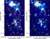 |
Fig. 1 Contour maps of the integrated emission for the [O i] 63 μm and [C ii] 158 μm lines (left and right panels, respectively), superimposed on an Spitzer/IRAC image centered on 4.5 μm. The (red) dashed line delineates the boundaries of the region mapped with Herschel/PACS. In the right panel the positions of the most prominent Class 0 (green filled circles), Class I sources (green filled triangles) and outflows discussed in the text are potted for reference. Filled (red) squares labeled (a–i) correspond to positions of spectra displayed in Fig. 2. Contour levels start at 8 × 10-15 erg cm-2 s-1 and increase logarithmically in steps of 0.5 dex. |
2. Data reduction
Observations of NGC 1333 were performed as part of the OT1 program entitled “A Herschel Study of Star Formation Feedback on Cloud Scales” (H. Arce, P.I.) and data were retrieved from the Herschel Science Archive (HSA)1. They consist of two maps obtained with the PACS spectrograph (Poglitsch et al. 2010) in line-scan mode, centered on the rest wavelength of the [O i] 3P2–3P1 and the [C ii] 2P3/2–2P1/2 lines (63.185 and 157.741 μm, respectively). The total duration of observations for each map is 30 744.0 s (~8.5 h). The [O i] and [C ii] lines were observed with the B3A and R1-long PACS bands, respectively, in unchopped-line-spectroscopy mapping mode. [O i] and [C ii] maps are centered on αJ2000 = 03h29m03 3, δJ2000 = + 31d20m499 and αJ2000 = 03h29m032, δJ2000 = + 31d20m398, respectively. Each map consists of tiling the 5 × 5 PACS footprint within a grid consisting of 8 raster lines and 17 raster columns, with a raster step of 41″ in each direction. The total mapped area corresponds to ~11.5′× 6′ and covers almost the entire NGC 1333 star-forming region.
Observations were processed with version 13 of the Herschel interactive processing environment (HIPE), using the CalTree 69 pipeline, provided by the Herschel Science Center. At the end of the reduction/calibration process, individually mastered observations were combined into mosaics using the task specInterpolate. The resulting mosaics have a spaxel size of 4.7″ with fluxes being interpolated using a Delaunay triangulation from the original input footprints, which are then projected onto an equidistant wavelength grid.
After this point data were treated with custom scripts. Line fluxes were calculated with simple integration on each spaxel after removing a first-order polynomial baseline. For [O i], line centroids were determined by Gaussian-fitting the emission-line components on each spaxel. Line maps were reconstructed by reprojecting the calculated properties on a regular grid with a pixel size equal to that of the original cubes.
The design values for the PACS spectral resolution at 63 and 157 μm correspond to R ~ 3500 and 1200, which translates into a velocity resolution of ~85 and 250 km s-1 for the [O i] and [C ii] line maps, respectively. In-flight calibrations and other observations have shown that in practice the spectral resolution values can be as low as 130 km s-1 for the [O i] line (e.g., Nisini et al. 2015). We here adopted a nominal resolution value of 100 km s-1 for the [O i] line. The specInterpolate task oversamples the wavelength grid into 3.8 km s-1 wide bins, but features at this velocity resolution can only be considered as artifacts.
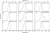 |
Fig. 2 Continuum-subtracted spectra of the [O i] line at 63 μm extracted from single PACS pixels on selected positions denoted with filled (red) squares in the right panel of Fig. 1. Coordinates corresponding to different locations are given at the top right of each panel. The dashed line indicates the [O i] cloud velocity at 24 km s-1 or 63.191 μm (see also Fig. 4). |
3. Line emission
Here we discuss the spatial distribution of the [O i] and [C ii] lines and through this associate their excitation to different processes. We examine the [O i] line profiles and employ velocity-channel and line-centroid maps to study different line-shape characteristics and their correspondence to the line maps.
3.1. Overall morphology
The integrated line-emission maps of [O i] and [C ii] are shown in Fig. 1, superimposed on a Spitzer/IRAC band 2 image that is centered on 4.5 μm. The emission in both maps is dominated by a strong peak toward the northeast, at a location coincident with the star IRAS 03260+3111(E). This late G-type star (Doppmann et al. 2005) is associated with the prominent reflection nebula SVS 3. The [C ii] line at 157 μm is linked to energetic (X-ray and ultraviolet) radiation fields in photon-dominated regions (PDRs; e.g., Dionatos et al. 2013; Green et al. 2013), which is also suggested by diffuse near-infrared H2 emission (Greene et al. 2010). While some morphological features such as the jet-like pedestal extending to the west from IRAS 03260+3111(E) appear to have a [C ii] counterpart, the large-scale [C ii] distribution in Fig. 1 shows little or no association with the extended H2 emission traced by the Spitzer/IRAC background image. The [C ii] emission is dominant in the north and remains prominent in the vicinity of HH12 complex to the northwest, but it gradually fades toward the south and becomes barely detectable, with the exception of very localized patches of emission. The morphology of the [O i] distribution in contrast shows significant structures and remains prominent across most of the mapped area. Both theoretical and observational studies associate the [O i] emission with strong shocks under the influence of protostellar jets (e.g., Hollenbach & McKee 1989; Nisini et al. 2015; Green et al. 2013; Dionatos et al. 2013). In the maps presented in Fig. 1, [O i] delineates almost every single outflow, as traced by H2 emission in the Spitzer/IRAC image, so that its excitation can be attributed to the influence of shocks. There are very few exceptions to this phenomenology, where H2 emission has no apparent [O i] counterpart, but this may be related to the local shock conditions or the sensitivity of the [O i] maps. The association between the [O i] emission morphology with the H2, CO and other jet or outflow tracers is discussed extensively in Sect. 3.3.
Additional evidence of the association of the [O i] with shocks induced by protostellar jets comes from the emission-line morphology, presented in Fig. 2. In this, the [O i] lineshape has a noticeable diversity corresponding to different locations across NGC 1333. The simplest shape (panel a of Fig. 2) corresponds to the emission around IRAS 03260+3111(E). The line appears almost symmetric, but is slightly shifted to the [O i] rest velocity (more on the rest-velocity definition in Sect. 3.2) and has clear wings at the base. Lines presented in all other panels of Fig. 2 correspond to outflow regions, and their amplitude is a factor ~30 lower than in panel a. In all cases the line center is shifted with reference to the [O i] rest velocity by as much as ±50 km s-1. Similar or even higher velocity shifts have been reported in the study of [O i] emission around embedded protostars by Nisini et al. (2015) for the sources IRAS 4A and BHR 71. The [O i] line-morphology is often complex and displays multiple peaks (e.g. Fig. 2, panel f), indicating the action of multiple jet components within the same spaxel. Signatures of high-velocity gas appear as extended line-wings (e.g. panels b, i) or as separated peaks, partly detached from the main line body (e.g. panels d, g). The latter morphology is typically associated with high-velocity bullets in outflows (e.g., Kristensen et al. 2012; Dionatos et al. 2010b). The velocity of the gas suggested by the extended line-wings reaches ±300 km s-1 in some cases (e.g., panel b).
Given the large velocity shifts observed throughout the map, we attempt to examine the spatial distribution of excited gas at different velocities in Fig. 3, although the spectral resolution of the [O i] line is limited (see Sect. 2). The selected velocity bins are coarse, ranging from 0.1 μm or ~50 km s-1 around the body of the line to 0.3 μm (~150 km s-1) in the outer parts to increase the signal-to-noise ratio in the high-velocity wings. The strongest feature in the velocity channel maps (Fig. 3) remains the emission around SVS 3, which is prominent in all cases. For blueshifted gas at the highest velocities [−298, −100] km s-1 the most prominent features are associated with the HH 12 object to the northwest and with the HH 7-11 outflow in the south. Symmetrical redshifted features can be identified between ~80 and 300 km s-1 bins, which for HH 7-11 are more pronounced. The morphology seen in the maps pertaining to velocities closer to the line center is more confused. Elongated blue- and redshifted emission features corresponding to outflow lobes can be distinguished toward the IRAS 2 and IRAS 4 regions (to the southwest and southeast of the maps, respectively). The locations where the emission peaks also show noticeable changes across different velocity-channel maps, indicating a significant shift in the location of the linecenters, where the peak of emission originates.
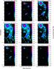 |
Fig. 3 Velocity channel maps of the [O i] emission in NGC 1333. For the extreme blue- and redshifted velocity wings (top left and bottom right panels, respectively) line emission is integrated over 0.3 μm or ~140 km s-1 while for the rest of the maps channel spacing corresponds to 0.1 μm or ~45 km s-1. Integrated flux per channel is encoded in the corresponding color bars of each panel and levels are adjusted to maximize the contrast and render weaker features visible. |
3.2. Gaussian line centroids
As discussed in the previous paragraphs, the [O i] line centers appear to be shifted to velocities of ±50 km s-1 or more (Fig. 2), which is also reflected in the spatial distribution of the [O i] emission in the velocity channel maps of Fig. 3. We here extend the analysis of the velocity structures mapped with the [O i] line by refining the determination of the position of the line centers. To this end, each line was Gaussian-fitted and the line centroid was determined from the Gaussian peak centroid. The error in determination of the Gaussian peak line centroids is given by the relation (Garnir et al. 1987)  (1)where f is the full-width at half maximum (FWHM) of the line and a is the relative line amplitude (the ratio of the line amplitude at the peak bin with respect to the full line). When the instrumental FWHM of 100 km s-1 is taken as a useful resolution limit for our observations (see also Sect. 2) and with a relative line amplitude of a = 0.5, the error in the derivation of Gaussian peaks is of the order of 5.5 km s-1 according to Eq. (1). This limit can be improved and may reach below 5 km s-1 when the relative line amplitude is higher, for example, in the region around SVS 3 (see Fig. 2). We therefore find that line-centroids can retrieve details in velocity that are beyond the design capabilities of Herschel/PACS.
For estimating the velocity centroid displacements, we first calculated the velocity shifts based on the Gaussian-defined line centroids for all spaxels of the [O i] map, and in Fig. 4 we present their number distribution. In the same figure, the rest frequency of the [O i] line at 63.185 μm (dashed line) is also shown. The peak of the [O i] line-centroid distribution lies at 63.192 μm, which corresponds to a shift of 0.005 μm or a Doppler-shift of ~24 km s-1. Examining the line-centroid distribution for different regions of the [O i] map, we find that the peak of the distribution is dominated by the PDR-excited emission toward the north (above the Dec = 31°:19′:00″ line) where emission lines are much stronger and the line-centroids can be more accurately defined. Below that limit, in the region where the emission is dominated by outflows, the distribution is less pronounced but remains symmetrical around the same velocity.
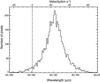 |
Fig. 4 Number distribution of the [O i] line centroids running for all spaxels of the NGC 1333 map (see Fig. 1) in bins of 1 km s-1. The dashed line indicates the location of the rest wavelength for the 3P2–3P1 transition of [O i] at 63.1852 μm. The distribution is to a good approximation normal and peaks at 63 191 μm, corresponding to a velocity shift of ~24 km s-1, which is taken as the [O i] rest velocity of the system. |
The systemic velocity of NGC 1333, as determined through a number of studies on water masers and outflows, is found to be +8 km s-1 (e.g., Rodríguez et al. 2002; Choi 2005; Persson et al. 2012). This is a factor of 3 lower than the rest velocity of the [O i] as defined through the number distribution of the line centroids. The reason for this discrepancy is not yet clear. It is possible that systematics may have been introduced during the last phase of the data reduction, were the spaxels are projected onto an equidistant wavelength grid. All steps of the reduction involving wavelength calibration of the PACS data were double-checked, and to the best of our knowledge, no problems were found. The [O i] rest-velocity measurement, is exact with respect to the observations discussed here, however, and is therefore used throughout the paper (see also Sect. 3.3).
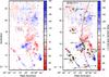 |
Fig. 5 Left: map of the velocity shift observed in the [O i] line centroids with respect to its rest velocity. Color-coding for each pixel corresponds to blue – and redshifts, as indicated on the corresponding bar on the right side of the plot. Right: a finder chart based on the left-hand side map, showing outflows (dashed arrows) and embedded (Class 0 and Class I) sources (open circles and triangles, respectively). The dotted X in the north shows the borderline between the low-velocity blue- and redshifted gas tracing the photodissociative wind from IRAS 03260+3111(E) (the position of the source is marked with a star). |
3.3. Line-centroid maps
The spatial distribution of the [O i] line centroids is presented in the left panel of Fig. 5. To assist the discussion of the great amount of details revealed in this map we provide a finder-chart in the right panel of Fig. 5. Starting from the north at the top of the map and around SVS 3, the line centroids reveal a slow ±10 km s-1 wind associated with the PDR region associated with IRAS 03260+311 (E). The emission appears to be red- and blueshifted toward the east and west with respect to the position of the system IRAS 03260+3111(E) with a symmetry axis running almost north-south (denoted with the dotted-X in Fig. 5). The velocities traced in the map are compatible with the velocities predicted to be generated by photo-evaporative winds in protostars (e.g., Woitke et al. 2009; Gorti & Hollenbach 2009). This interpretation is also consistent with the maximum of the [C ii] line emission which is observed in the same region (e.g., Greene et al. 2010).
At the same declination and extending directly to the west, a series of blueshifted knots from the Class I protostar IRAS 03260+3111(W) (Evans et al. 2009) delineates the prominent jet that also appears in the blueshifted channels of Fig. 3 (dashed arrow). The morphology becomes more confused to the northwest around the region of HH12, where the bulk of the emission is blueshifted. The cluster of high-velocity (>30 km s-1) knots associated with the HH12 object corresponds to a series of resolved knots observed in the near-IR H2 emission (Hodapp & Ladd 1995), but also to blueshifted CO emission (Knee & Sandell 2000; Curtis et al. 2010). HH12 also shows significant [C ii] emission extending to the south where the Spitzer/IRAC image depicts an emission-free cavity, which is most likely associated with the Class I source SK26 (Sandell & Knee 2001; Enoch et al. 2008). Class I sources are copious emitters of energetic photons (e.g., X-rays, Güdel et al. 2007) that can excite and ionize the surrounding gas. The blueshifted emission is only interrupted by a long arc-shaped stream of redshifted knots running roughly north-south (dashed line), which is probably symmetric with a series of blueshifted knots extending to the far south. This southward-extending structure most likely corresponds to the extended, blueshifted CO emission observed and attributed to SVS13B in Curtis et al. (2010), so in this configuration the structure represents a single long outflow running north-south throughout the [O i] map.
Toward the center of the map and slightly to the east, the HH6 clump displays patchy entangled blue- and redshifted emission that is linked to outflow activity from four Class I protostars, which are embedded in this region. The angular resolution of the maps is not sufficient to distinguish individual outflows, but patches of shocked, H2 emission toward the south have been kinematically associated with HH6 (Raga et al. 2013).
In south, located close to the map center, in the region where the outflow emission dominates, the high-velocity peaks in the velocity-centroid maps show an astonishing degree of symmetry between blue and redshifted structures. The most prominent feature, HH 7-11, shows a series of high-velocity, blueshifted knots that appear in reflection in the symmetric redshifted lobe that extends to the northwest. The area around the interface between the HH 7-11 and the redshifted counter-lobe is packed with a number of Class 0 and Class I protostars that drive overlapping and possibly interacting outflows (see also panel f in Fig. 2). The bipolar outflow as a whole is associated with the Class 0 source SVS13A, which is located at the center of symmetry between the lobes. The chain of high-velocity peaks follows a wavy sinusoidal pattern, indicating a strongly precessing outflow. These structures may also correspond to a number of different outflows that are driven by more than one source. Other embedded protostars in the field are associated with prominent outflow structures. SVS13B probably drives the large-scale outflow discussed in the previous paragraph, and SVS13C is associated with the bipolar outflow extending to the northeast-southwest (dashed arrows in Fig. 5, see also Plunkett et al. 2013). Directly to the south, we confirm the tentative association from Plunkett et al. (2013) of a narrow bipolar outflow to the Class 0 source SK14.
To the southwest, the line-centroid map reveals two almost parallel bipolar outflow structures. The more extended of the two is associated with the north-south IRAS 2A outflow (Plunkett et al. 2013; Curtis et al. 2010). Attributing a driving source to the smaller bipolar structure is however not straightforward as there are no known embedded sources around the center of symmetry. The nearest embedded protostar is the Class I source IRAS 2B, which is located at the same spot as the blueshifted emission. We tentatively associate this outflow structure with IRAS 2B as presented in Fig. 5. In this configuration, the projected directions of the blueshifted emission from IRAS 2A and IRAS 2B overlap, but different outflow configurations may be valid if IRAS 2B is an embedded binary protostar (Tobin et al. 2016). A third outflow in the region that is associated with the IRAS 2A binary extending east-west (Tobin et al. 2015; Plunkett et al. 2013) is not clearly detected in the line-centroid maps, with the exception of a redshifted emission patch at the tip of the red arm.
In the southeast, the narrow but extended jet-like emission is associated with the source IRAS 4A. The binary nature of the source (Tobin et al. 2016) may explain the different projected angle between the inner and outer high-velocity knots. The region around this corner of the map is speckled with a number of smaller isolated high-velocity clumps which can be attributed in multiple configurations to a number of embedded sources lying in the same area. Information on the proper motions as derived from the H2 knots observed in the mid-infrared (Raga et al. 2013) is often complex, confusing, and in some cases suggests that some of these clumps may be associated with larger outflow structures originating further up to the north, around HH 6 or beyond. Based on pure symmetry assumptions, we tentatively associate four such clumps into two bipolar outflow schemes linked to IRAS 4D (see Fig. 5). Finally, at the very south of the [O i] map and following the suggestion of Plunkett et al. (2013) we associate a series of clumps aligned east-west with the Class 0 source SK1.
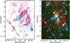 |
Fig. 6 Left: the outflow structures as recovered by the [O i] centroid analysis, in comparison with CO (1–0) interferometric map of Plunkett et al. (2013). Color levels are the same as in Fig. 5 and the frame focuses on the southern star-forming complex of NGC 1333. Right: [O i] line-centroid velocity shift superimposed on an IRAC 4.5 μm image showing the close spatial coincidence between the two shock tracers. Contour levels start at 5 km s-1 and increase in 10 km s-1 increments for both blue- and redshifted channels. |
It is instructive to study the kinematics of the [O i] line-centroid maps in comparison with other common jet and outflow tracers to access the quality of the line-centroid method and role of the [O i] emission as a jet and outflow tracer. In the left panel of Fig. 6 we present the 12CO J = 1 → 0 outflow map of Plunkett et al. (2013) obtained with CARMA, superimposed on the [O i] velocity centroid map. The angular resolution of the CARMA map is ~5″, which is almost identical to the ~4.5″ spaxel scale of the [O i] maps of this work. The velocity resolution of the CARMA maps, however, is a factor of 20 better than the limit reached with the velocity centroid method and can therefore reliably trace more detailed velocity structures. The maps shown in Fig. 6 display very similar morphologies, tracing consistently every large-scale outflow structure. The high-velocity peaks of the [O i] map fill-in the hollow donut-shaped outflow lobes and cavities of the CO emission, rendering the two maps complimentary. An exception to this general trend is the redshifted lobe extending to the northeast from IRAS 2A, which seems to correspond to an emission cavity as seen in both the H2 and [O i] emission. We note that the CO J = 1 → 0 observations of Plunkett et al. (2013) pertain only low-velocity gas (up to ±10 km s-1), while higher velocities have been reported for higher J CO transitions (e.g. Bachiller et al. 2000). Surprisingly, the low-velocity substructures in the [O i] map, such as the entangled blue- and redshifted emission at the tip of the HH 7-11 outflow or the similarly entangled emission to the NE lobe from IRAS 4A correspond almost exactly to features in the CO maps. In addition, CO clumps that are observed around the HH 7-11 outflow and are denoted as F1–F5 in Plunkett et al. (2013) correspond to regions where the [O i] changes velocity sign from blue- to redshifted and vice versa.
As mentioned earlier on, the distribution of [O i], with very few exceptions, closely follows the distribution of the mid-infrared H2 emission (Fig. 1). In the right panel of Fig. 6 we present the line-centroid velocity distribution of the [O i] in comparison to the H2 emission. The [O i] emission not only agrees with the H2 distribution but the [O i] velocity peaks are centered with great accuracy on the locations of the H2 knots. We note that the IRAS 2A east-west outflow which is one of the dominant bipolar outflows in CO not traced in [O i], also has no visible counterpart in the Spitzer H2 image. The east-west flow from IRAS 2A apparently produces no shocks and remains purely molecular to large distances, which is possibly associated with the very low momentum carried by this structure (Plunkett et al. 2013, see also Table 1). As a comparison, the very young outflow from HH 211 appears to be purely molecular at the base close to the protostar, but shows strong H2 emission from shocks farther out (e.g., Dionatos et al. 2010a; Tappe et al. 2008).
Summarizing, the [O i] emission appears to be complimentary, filling the CO emission in a jet-entrainment fashion, and closely follows the H2 knot distribution, showing that it is excited in shocks. [O i] is probably produced in situ, breaking apart O-bearing molecules such as CO or H2O in dissociative J-shocks (Flower & Pineau Des Forêts 2010), and the correlation between the high-velocity [O i] emission with the H2 knots support this assumption. The same argument may explain the lack of [O i] emission in fainter H2 knots observed in a few cases, indicating that either the shock velocity and density is not high enough or that the shock may not be dissociative but continuous (C-type). The [O i] distribution strongly suggests that almost every single shock observed in NGC 1333 is either a pure J-type shock or that there is at least a dissociative component at each shock location, which consistent with a bow-shock topology (Hollenbach 1997). In this respect, outflows can represent entrained ambient gas, generated at a mixing-layer interface along the sideways extending bow-shock flanks in an internal working-surface configuration (Raga & Cabrit 1993).
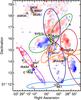 |
Fig. 7 As in Fig. 5 but focusing on the southern two-thirds of NGC 1333. Positions of embedded sources in the cloud are indicated with circles (Class 0) and triangles (Class I) and corresponding names are given for each source (the source labeled as SST next to IRAS4A corresponds to SSTc2dJ032910.65+311340.0). Colored ellipses delineate the outflow lobes attributed to embedded protostars in the work of Plunkett et al. (2013), and also employed here for the description of the outflow dimensions. |
Comparison of jet momentum and energies calculated from the [O i] line emission.
4. Dynamics and kinematics of the [O i] jets
Based on the [O i] emission maps in the following we describe the methods for determining the mass, momentum, and energy, and also the outflow dynamical timescales and the mass flux of the underlying protostellar jets.
To facilitate comparisons with the CO J = 1 → 0 emission we calculated the [O i] momentum for the outflows defined from the corresponding CO maps, using the reported source-position and outflow geometrical properties (see Tables 2 to 4 in Plunkett et al. 2013). We did not consider any tentative outflows such as the flows C1 to C4 and the monopolar flow from the protostellar source IRAS2B in Plunkett et al. (2013). The geometry adopted from the CO outflows in Plunkett et al. (2013), superimposed on the [O i] velocity map is shown in Fig. 7. The ellipses surrounding the CO outflows exceed in some cases the limits of the [O i] map toward the west (Fig. 7), but this has negligible influence on our calculations as there is little [O i] emission extending in this direction.
4.1. Mass, momentum and energy
The momentum generated by the [O i] outflow is key to our understanding of the effect of the atomic jets on the cloud environment. Owing to the large velocity dispersion observed in the [O i] line (Fig. 3), we calculated the momentum using the following relation: ![Mathematical equation: \begin{equation} P_{[\ion{O}{i}] } = \sum_{v_{\rm bin}} M_{v_{\rm bin}} \lvert v - v_{r} \rvert \end{equation}](/articles/aa/full_html/2017/01/aa29179-16/aa29179-16-eq44.png) (2)where the sum acts over the mass per velocity bin, v is the mean velocity for each velocity bin and vr is the rest velocity for the [O i] as defined in Sect. 3.3. The mass per velocity bin (Mvbin) is derived from the [O i] luminosity per velocity bin, adopting the relation from Dionatos et al. (2009):
(2)where the sum acts over the mass per velocity bin, v is the mean velocity for each velocity bin and vr is the rest velocity for the [O i] as defined in Sect. 3.3. The mass per velocity bin (Mvbin) is derived from the [O i] luminosity per velocity bin, adopting the relation from Dionatos et al. (2009): ![Mathematical equation: \begin{equation} M_{v_{\rm bin}} = \mu m_{\rm H} \frac{L_{v_{\rm bin}}[\ion{O}{i}]}{h\nu A_if_iX[O]}\cdot \label{eqn:2} \end{equation}](/articles/aa/full_html/2017/01/aa29179-16/aa29179-16-eq48.png) (3)In Eq. (3), μ = 1.4 is the mean particle weight per H nucleus, mH is the mass of the hydrogen atom, Ai is the Einstein coefficient for spontaneous emission, fi is the relative occupation of level i, and X[O] is the abundance of atomic oxygen. The values for X[O] vary from 10-3.52 to 10-3.24 (see Rab et al. 2016, and references therein) and therefore introduce minor uncertainties in the mass calculations. A major contribution to the uncertainties involved in the mass derivation originate from the relative level occupation factor fi in the denominator of Eq. (3), which depends on the [O i] excitation conditions, and in particular from the kinetic temperature, the density, and the nature of the colliders.
(3)In Eq. (3), μ = 1.4 is the mean particle weight per H nucleus, mH is the mass of the hydrogen atom, Ai is the Einstein coefficient for spontaneous emission, fi is the relative occupation of level i, and X[O] is the abundance of atomic oxygen. The values for X[O] vary from 10-3.52 to 10-3.24 (see Rab et al. 2016, and references therein) and therefore introduce minor uncertainties in the mass calculations. A major contribution to the uncertainties involved in the mass derivation originate from the relative level occupation factor fi in the denominator of Eq. (3), which depends on the [O i] excitation conditions, and in particular from the kinetic temperature, the density, and the nature of the colliders.
Constraining the excitation conditions requires observations of more than a single transition of an atom, and the only additional data available in this work come from the [C ii] maps. As discussed in Sect. 3.2, the 157 μm line is excited in radiative and not in collisional processes, and can therefore provide little information on the [O i] excitation. For the following analysis we therefore need to rely on certain assumptions and employ results of similar studies found in the literature (e.g., Liseau & Justtanont 2009; Nisini et al. 2015). In a recent work employing [O i] observations excited in protostellar jets around five embedded sources with Herschel, Nisini et al. (2015) employed non-thermal equilibrium (NLTE) models together with additional data on the 3P1–3P0 [O i] line at 145 μm to study the possible excitation conditions of [O i]. Summarizing the main results of this analysis, Nisini et al. (2015) found that while the density of colliders is rather well constrained (ranging between 104−105 cm-3), the nature of the colliders (atomic or molecular hydrogen) can affect the 63 μm [O i] emissivity by a factor ranging between 2 and 5. In an order study, Liseau & Justtanont (2009) demonstrated that the emissivity of the 63 μm line can vary up to a factor of three for kinetic temperatures higher than 300 K, while in the same study they find that the excitation of the [O i] 63 μm line typically traces kinetic temperatures of ~1000 K.
As pointed out by Liseau & Justtanont (2009), the 63 μm line is optically thin for H2 column densities of ~1019 cm-2. On similar grounds, Nisini et al. (2015) used the radiative transfer code RADEX (van der Tak et al. 2007) and estimated that an appreciable opacity change for the 63 μm line occurs for column densities higher than 1022 cm-2. Direct column density measurements for all major outflows in NGC 1333 using Spitzer spectral-line mapping of H2 rotational transitions show a variation between ~1019 cm-2 and ~1018 cm-2 for the warm and hot H2 components, respectively (Maret et al. 2009). Given the close association between the [O i] and the H2 emission (see Sect. 3.3), we can safely assume that there are no significant optical depth effects affecting the [O i] 63 μm line so that the line emission probes the total volume of gas. Comparisons of the 63 and 145 μm [O i] lines close to embedded protostars and farther out show that there is no appreciable variation, which is interpreted as an indication that there is no significant extinction of the 63 μm line even deep within the protostellar envelopes (Nisini et al. 2015). Summarizing, the mass derivation based on the [O i] luminosity can vary up to a factor of ~10 as a result of the uncertainties in the local excitation conditions, but there should be no appreciable losses due to extinction or optical depth effects.
The jet energy traced by the [O i] line can be derived according to the following relation: ![Mathematical equation: \begin{equation} E_{[\ion{O}{i}] } = \frac{1}{2}\sum_{v_{\rm bin}} M_{v_{\rm bin}} \lvert v - v_{r} \rvert^{2} \end{equation}](/articles/aa/full_html/2017/01/aa29179-16/aa29179-16-eq64.png) (4)where the mass per velocity bin is defined in Eq. (3) and velocities follow the same notation as for the momentum. The uncertainties in the mass derivation discussed above also affect the estimation of the energy deposited by the outflows. The derived [O i] values for the momentum and energy are reported separately in Table 1 for each outflow source and lobe. In the same table and to facilitate direct comparisons, we also provide the corresponding CO momentum and energy values from Plunkett et al. (2013).
(4)where the mass per velocity bin is defined in Eq. (3) and velocities follow the same notation as for the momentum. The uncertainties in the mass derivation discussed above also affect the estimation of the energy deposited by the outflows. The derived [O i] values for the momentum and energy are reported separately in Table 1 for each outflow source and lobe. In the same table and to facilitate direct comparisons, we also provide the corresponding CO momentum and energy values from Plunkett et al. (2013).
[O i] mass flux, jet dynamical timescales.
Properties of jets, outflows and their corresponding sources.
4.2. Mass flux, dynamical timescale
To calculate the mass flux, we followed the prescription of Dionatos et al. (2009), which has also been applied in a number of similar cases (e.g. Dionatos et al. 2014; Nisini et al. 2015). According to this, the mass flux can be estimated from the following relation: ![Mathematical equation: \begin{equation} \dot{M}_{[\ion{O}{i}]} = \mu m_{\rm H} \frac{L_{[\ion{O}{i}]}}{h\nu A_if_iX[{\rm O}]} \times t_{\rm dyn}^{-1}. \end{equation}](/articles/aa/full_html/2017/01/aa29179-16/aa29179-16-eq82.png) (5)Similar to the previous section, the mass determination is based on the [O i] luminosity, with the difference that we now consider the total luminosity of gas confined within a given volume. The uncertainties related to the [O i] excitation and the influence of optical depth and extinction effects discussed in Sect. 4.1 also apply in this case. To estimate the mass flux, we define a dynamical scale from the projected length of the outflows and the tangential velocity of the emitting gas according to the following relation:
(5)Similar to the previous section, the mass determination is based on the [O i] luminosity, with the difference that we now consider the total luminosity of gas confined within a given volume. The uncertainties related to the [O i] excitation and the influence of optical depth and extinction effects discussed in Sect. 4.1 also apply in this case. To estimate the mass flux, we define a dynamical scale from the projected length of the outflows and the tangential velocity of the emitting gas according to the following relation:  (6)Estimations of the tangential velocity rely on accurate proper-motion measurements that are often derived from gas tracers different from those employed to derive the mass flux. We here employed the measurements of Raga et al. (2013), which are based on a multi-epoch study of H2 knots observed with Spitzer. Given the close morphological correlation of the [O i] and H2 emission, we assumed that the proper motions derived by the latter also describe the [O i] flow well. To be consistent with the analysis of the previous paragraph, we adopted for the definition of projected outflow lengths the dimensions of the CO outflows from Plunkett et al. (2013). The values of the parameters employed in the calculation of the dynamical timescales (projected length and tangential velocity), along with the derived values for the oxygen mass flux are reported in Table 2. To facilitate direct comparisons with the physical quantities of Table 1, values are reported separately for the blue- and redshifted lobes.
Alternatively, the mass flux of outflows can be directly estimated according to the relation showing that the mass-loss rate is directly proportional to the [O i] luminosity (Hollenbach & McKee 1989): ![Mathematical equation: \begin{equation} \frac{\dot{M}_{[\ion{O}{i}]_{\rm shock}}}{ M_{\odot}\,{\rm yr}^{-1}}= \frac{10^{-4} \times L_{[\ion{O}{i}]} }{ L_{\odot}}\cdot \label{eqn:6} \end{equation}](/articles/aa/full_html/2017/01/aa29179-16/aa29179-16-eq84.png) (7)This relation assumes that all [O i] emission is generated in dissociative J-type shocks, an assumption that is observationally supported by an increasing volume of studies (e.g., Dionatos et al. 2013; Nisini et al. 2015). As discussed in Nisini et al. (2015), the relationship considers a single shock interface where the velocity of the jet is assumed to be equal to the shock velocity. Based on the velocities of jets from evolved protostars, Nisini et al. (2015) assumed that the shock velocity is in fact 3–6 times lower than that of the jet. This factor would then cancel the effect of multiple shocks within a jet lobe, so that Eq. (7) holds as is and needs no further corrections. Values for the [O i] mass flux estimated by Eq. (7) are reported in Table 2, together with previous estimations.
(7)This relation assumes that all [O i] emission is generated in dissociative J-type shocks, an assumption that is observationally supported by an increasing volume of studies (e.g., Dionatos et al. 2013; Nisini et al. 2015). As discussed in Nisini et al. (2015), the relationship considers a single shock interface where the velocity of the jet is assumed to be equal to the shock velocity. Based on the velocities of jets from evolved protostars, Nisini et al. (2015) assumed that the shock velocity is in fact 3–6 times lower than that of the jet. This factor would then cancel the effect of multiple shocks within a jet lobe, so that Eq. (7) holds as is and needs no further corrections. Values for the [O i] mass flux estimated by Eq. (7) are reported in Table 2, together with previous estimations.
5. Discussion
The oxygen maps presented in the previous sections are of comparable quality in terms of angular and velocity resolution to the CO maps of Plunkett et al. (2013), which are of unprecedented detail that has not been matched so far, given the extent of the area covered. Within this area we consistently derived the dynamical and kinematical properties for the atomic and molecular components of seven bipolar configurations where jets and outflows can be strongly associated. For the analysis we followed constant definitions for the loci of molecular and atomic ejecta and used consistent methods on homogeneous datasets to derive their properties. Therefore, the analysis of these data for the first time provides a unique opportunity to study the relation between the atomic and molecular ejecta, but also to assess the influence of atomic jets on their immediate surroundings and estimate their feedback on large star-forming core scales.
5.1. Relation between atomic jets and molecular outflows.
The kinematic and dynamical properties of the bipolar [O i] jets and CO outflows discussed in the previous sections along with the physical properties of their corresponding driving sources are summarized in Table 3. In Fig. 8 we compare the momentum and energy between the atomic and molecular ejecta (center and left panels, respectively). While the CO and [O i] momenta appear to closely correlate, the momentum carried along the [O i] line represents only a fraction of ~1% compared to the momentum corresponding to the CO emission. On the other hand, the energy carried by the atomic gas corresponds to 50–100% of the energy measured in the molecular component. In the right panel of Fig. 8, we display the correlation of the [O i] and CO emission with the bolometric luminosity of the driving sources. We note that the star symbols correspond to the east-west directed outflow of the source IRAS 2A, which is rather a peculiar case and is considered here as an outlier. While similar correlations for the momentum flux of molecular flows are well known (e.g., Bontemps et al. 1996; Dionatos et al. 2010a), this is the first time that such a correlation is shown to hold also for the [O i] ejecta emission related to embedded protostars, and it provides possible indications that the mass-loss phenomena also traced in atomic lines are directly linked to the accretion processes occurring very close to protostars.
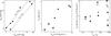 |
Fig. 8 Comparison of the energy and momentum (left and center panels, respectively) derived from the analysis of the [O i] emission with the corresponding CO values from Plunkett et al. (2013), as listed in Table 3. The CO and [O i] momenta (empty and filled circles, respectively) are plotted against the embedded-source bolometric luminosities in the right-most panel. In the same panel, filled and empty stars correspond to the east-west outflow of source IRAS 2A. |
If we assume that the bona-fide ejecta from protostars along all evolutionary stages is atomic, as evidenced from the micro-jets of T Tauri stars (e.g., Agra-Amboage et al. 2009), then the observed [O i] emission can very well represent the same atomic gas. In such a scenario, the molecular outflow emission traced in the CO lines would correspond to jet-entrained ambient gas in the surrounding environment of forming stars. While the physical structure and appearance of the molecular outflows would be dictated by the dominant modes of interaction between the underlying atomic jet with the surrounding medium (Arce et al. 2007), a casual link between the two flows would translate into conserving the momentum. Given that the [O i] velocity is ~10 times higher than the CO gas, the [O i] momentum is ~1% of the CO and that the total energy is equally distributed between the two flows, then we find that the CO appears to be 102–104 times more massive than the [O i] flow. In fact, the mass estimates in the previous paragraph support the higher mass ratio. To a first approach, these results suggest that the atomic jet does not possess enough momentum to drive the observed CO outflows. Alternatively, there may be significant [O i] reservoirs in the atomic flow where the gas is not excited and therefore not detected, an assumption that can hold in the context of [O i] excitation in shocks. In this scenario, the atomic gas is excited within a chain of shocks (internal working surfaces) and then cools radiatively in the post-shock zone. Therefore the cumulative size of the regions where the emission is arising would be very small compared to the total length of the flow (e.g., Hollenbach & McKee 1989). In this case, the [O i] emission measures only the gas excited in shocks, but not the oblique atomic gas between shocks that is not radiating, but is still moving at relatively high velocities and therefore significantly contributes to stirring up a mixing turbulent layer that is observed in molecular line emission. In such a scenario the [O i] emission observed can indeed support the assumption that the protostellar ejecta are predominantly atomic.
In the discussion above we assumed that the atomic gas mainly represents ejecta from a protostar that is consequently excited in shocks. There is enough evidence, however, that the observed shocks are dissociative J-type, indicating that at least some of the atomic gas is produced in-situ from the dissociation of oxygen-bearing molecules such as CO and H2O, at the location of the shocks. In this scenario, the oxygen production would strongly depend on the shock conditions such as the shock velocity and local density of the gas. Even though the shock conditions can have some affinity to the protostar, we would expect that the [O i] production and excitation in shocks would show little correlation to the properties of the forming star, which is in contrast with the correlation in the right panel of Fig. 8. In that case, the observed correlation would imply that each flow is directly linked to the driving source. The relation found between the momentum and the energy of the atomic and molecular ejecta agrees with the predictions of the numerical simulations performed by Machida (2014), who studied the formation and early evolution of protostars and considering a two-component (jet and outflow) protostellar ejecta in a nested configuration. In these simulations, the low-velocity outflow (uout < 50 km s-1) originates from the protostellar disk, is less collimated, and is rather constant during the main accretion phase. On the other hand, the high-velocity jet is highly variable because of episodic accretion events that can be created by a number of different instabilities in the accretion disk (e.g. gravitational instability, Vorobyov & Basu 2006; or a combination of gravitational instability and magnetic dissipation Machida et al. 2011). In this configuration, Machida (2014) demonstrated that the momentum generated by the episodic jet outbursts is always much lower than the more constant outflow, but the kinetic energy of the jet has spikes that exceed the energy of the outflows. As a result, the time-averaged values for the jet kinetic energy can account for a significant fraction of the outflow energy, but in contrast the jet momentum is too low to reach the outflow values even at the highest peaks.
5.2. Feedback of atomic jets onto the star-forming core
According to the properties measured from the [O i] emission, the atomic jet momenta can have little influence on the cloud compared to the contribution form outflows. The energy deposited by the atomic jets, however, cannot be neglected. Summing the jet and outflow energy output, the total energy feedback from protostellar ejecta to the cloud is ~1.1 × 1045 erg, or about 50% higher than the total energy transported by outflows alone (Plunkett et al. 2013). This value compares directly to the turbulent energy of the cloud (Eturb = 1.8 × 1045 erg) estimated in Plunkett et al. (2013) without accounting for the projected outflow inclination angles, and reveals the importance of the contribution of shocks in the cloud turbulence. Following the analysis of Plunkett et al. (2013), the assumed dynamical timescale for jet-driven outflows (5 × 10⁴ yr) is in excellent agreement with the mean of our estimates from Table 3. We find that the total luminosity from protostellar ejecta (outflows and jets) is Lej = Eej/tdyn ≈ 7 × 1042 erg s-1. The turbulent dissipation rate is given by Lturb = Eturb/tdiss, where tdiss = 5.7 × 10⁵ yr is the energy dissipation time (Arce et al. 2010). Comparing these two values we find a ratio Lej/Lturb ~ 7 that supports the conclusions from Plunkett et al. (2013) that outflows, but also jets, posses more than enough power to maintain turbulence, at least within the limits of the region studied here.
5.3. Mass flux from the atomic jets
The outflow mass flux derived Sect. 4.2 agrees well with the values derived in Nisini et al. (2015) for a number of outflows in different clouds. The outflow from IRAS 4A mass flux derived in Nisini et al. (2015) is ~1.5 × 10⁻⁷M⊙ yr-1, in excellent agreement with the values reported in Table 3. On average, the mass-flux values for NGC 1333 lie on the lower end compared to the values reported in Nisini et al. (2015). This difference can be attributed on the one hand to the lower tangential velocities adopted from Raga et al. (2013), and on the other hand to our assumption of fully atomic hydrogen as the main excitation agent. The mass flux estimations for the outflow from the source SVS13A, based on the near-infrared [Fe ii] and H2 lines (Davis et al. 2011) range from ~5 × 10⁻⁷ to 10-6M⊙ yr-1, comparable to the values derived here with the two different methods. It should be noted, however, that the values reported (Davis et al. 2011) are corrected for an average outflow inclination angle of 57.̊3 and extinction. A general trend observed in the current analysis is that the shock-derived mass flux can be up to a factor of 20 higher than the mass flux values calculated assuming a dynamical timescale. This is especially pronounced in cases of extended and confused lobes (e.g., for SVS13A and SVS13C), suggesting a higher-than-assumed number of shocks within each lobe that is not effectively canceled by the difference between the jet and shock velocities, as assumed in Nisini et al. (2015).
In the case that the [O i] emission represents bona fide ejecta from the protostar, we would expect to observe a clear trend in the mass flux of the atomic gas as a function of the evolutionary stage of a protostar, which would reflect the observed drop in accretion rates from Class 0 to Class II sources. In a study of the [O i] 63 μm emission with Herschel around five Class II protostars, Podio et al. (2012) reported mass fluxes of between 10-8 and 10-6M⊙ yr-1 with an average value of ~10-7M⊙ yr-1. Compared to the values reported here but also in Nisini et al. (2015), the jet mass flux shows only a minor decline between the embedded and the T Tauri phase, if any. These results support the two-component ejecta scenario of Machida (2014), which is also suggested by the difference in the momentum and energy between the jet-shocked emission and the outflows, as discussed in the previous sections.
6. Conclusions
We presented Herschel/PACS line maps of the NGC 1333 star-forming region based on line-scan observations of the [O i] and [C ii] lines at 63 μm and 157 μm, respectively. The emission from the two tracers peaks toward the north of the mapped region as a result of the energetic radiation from the source IRAS 03260+3111(E) which excites the SVS 3 reflection nebula. Significant [C ii] emission is also associated with the HH12 outflow region to the northwest. Toward the southern end of NGC 1333, the [C ii] emission weakens and the region is dominated by [O i] emission that is excited by jets from young protostars.
Our analysis focused on deriving the morphological, dynamical and kinematic properties of the atomic gas in the outflows as traced by [O i]. We then compared these properties to those traced by other outflow tracers such as CO. Our main results can be summarized as follows:
-
Oxygen lines display a high morphological diversity reflectinggas moving at a wide range of velocities. Extended line wingstrace in some cases velocities up to 300 km s-1. The continuous orsemidetached shape of the line-wings shows that the highvelocity gas can be associated to smoothly accelerated structuresor individual “bullets” of gas.
-
Notwithstanding the low velocity resolution of the [O i] maps velocity channel maps at bins of 50 km s-1 reveal outflow structures extending symmetrically to known protostellar sources. Channel maps show also the significant shifts in the [O i] line peaks, contributing to the local maxima in the different velocity bins.
-
A thorough estimation of the line-centroids as derived from Gaussian-fits to the [O i] lines provided velocity structures down to 5 km s-1, which is a factor of ~20 higher compared to the design-capabilities of Herschel/PACS.
-
The maps based on line-centroids trace velocity structures down to 5 km s-1 exposing even slow, symmetric flows from photo-evaporative winds.
-
The outflow structures revealed in the line-centroid maps show a great degree of detail and symmetries, providing important information necessary to associate individual flows to driving sources. Based on these maps we confirm a large number known, and propose a few new bipolar outflow structures and their associated driving sources.
-
The resolving power of the line-centroid maps in small, low velocity structures is comparable to CO interferometric maps of much higher velocity resolution, as revealed by copious comparisons. At larger scales the oxygen and CO emissions reveal very similar but often also complimentary outflow structures.
-
The [O i] line centroid velocity peaks follow closely the H2 emission indicating that oxygen is excited in shocks shocks.
-
The momentum carried by the [O i] represents only the ~1% of the momentum corresponding to the large-scale CO emission.
-
The energy traced by [O i] accounts for up to 100% of the energy measured in CO outflows.
-
Assuming that the oxygen emission represents jets from protostars which are also responsible for driving the CO outflows, then there must be a significant amount of atomic jet mass that is not excited in shocks. This can be consistent if the space between a chain of shocks (internal working surfaces) is filled with high velocity atomic gas which is not observable but creates interacts with the surrounding medium flow instabilities, creating much of the observed CO emission.
-
The momentum and energy estimates are in also agreement with the predictions of a nested jet/outflow structure simulations of Machida (2014), where the jet is linked to episodic accretion events, while the large-scale outflow is constant (non-episodic) and carries the bulk of the momentum.
-
The mass flux carried by the [O i] jets, estimated for evolved Class II sources shows no significant decline when compared to the values corresponding to embedded protostars, estimated in this work. This finding may give additional support of the two-component ejecta scenario discussed above.
Acknowledgments
This research was supported by the FFG ASAP-12 project JetPro* (FFG-854025) and in part by the EU FP7-2011 project under Grant Agreement No. 284405.
References
- Agra-Amboage, V., Dougados, C., Cabrit, S., Garcia, P. J. V., & Ferruit, P. 2009, A&A, 493, 1029 [NASA ADS] [CrossRef] [EDP Sciences] [Google Scholar]
- Arce, H. G., Shepherd, D., Gueth, F., et al. 2007, Protostars and Planets V, 245 [Google Scholar]
- Arce, H. G., Santiago-García, J., Jørgensen, J. K., Tafalla, M., & Bachiller, R. 2008, ApJ, 681, L21 [NASA ADS] [CrossRef] [Google Scholar]
- Arce, H. G., Borkin, M. A., Goodman, A. A., Pineda, J. E., & Halle, M. W. 2010, ApJ, 715, 1170 [NASA ADS] [CrossRef] [Google Scholar]
- Arce, H. G., Mardones, D., Corder, S. A., et al. 2013, ApJ, 774, 39 [CrossRef] [Google Scholar]
- Bachiller, R., Gueth, F., Guilloteau, S., Tafalla, M., & Dutrey, A. 2000, A&A, 362, L33 [NASA ADS] [Google Scholar]
- Bontemps, S., Andre, P., Terebey, S., & Cabrit, S. 1996, A&A, 311, 858 [NASA ADS] [Google Scholar]
- Choi, M. 2005, ApJ, 630, 976 [NASA ADS] [CrossRef] [Google Scholar]
- Curtis, E. I., Richer, J. S., Swift, J. J., & Williams, J. P. 2010, MNRAS, 408, 1516 [NASA ADS] [CrossRef] [Google Scholar]
- Davis, C. J., Stern, L., Ray, T. P., & Chrysostomou, A. 2002, A&A, 382, 1021 [NASA ADS] [CrossRef] [EDP Sciences] [Google Scholar]
- Davis, C. J., Cervantes, B., Nisini, B., et al. 2011, A&A, 528, A3 [NASA ADS] [CrossRef] [EDP Sciences] [Google Scholar]
- Dionatos, O., Nisini, B., Garcia Lopez, R., et al. 2009, ApJ, 692, 1 [NASA ADS] [CrossRef] [Google Scholar]
- Dionatos, O., Nisini, B., Cabrit, S., Kristensen, L., & Pineau Des Forêts, G. 2010a, A&A, 521, A7 [NASA ADS] [CrossRef] [EDP Sciences] [Google Scholar]
- Dionatos, O., Nisini, B., Codella, C., & Giannini, T. 2010b, A&A, 523, A29 [NASA ADS] [CrossRef] [EDP Sciences] [Google Scholar]
- Dionatos, O., Jørgensen, J. K., Green, J. D., et al. 2013, A&A, 558, A88 [NASA ADS] [CrossRef] [EDP Sciences] [Google Scholar]
- Dionatos, O., Jørgensen, J. K., Teixeira, P. S., Güdel, M., & Bergin, E. 2014, A&A, 563, A28 [NASA ADS] [CrossRef] [EDP Sciences] [Google Scholar]
- Doppmann, G. W., Greene, T. P., Covey, K. R., & Lada, C. J. 2005, AJ, 130, 1145 [Google Scholar]
- Eisloffel, J., & Mundt, R. 1997, AJ, 114, 280 [NASA ADS] [CrossRef] [Google Scholar]
- Enoch, M. L., Evans, II, N. J., Sargent, A. I., et al. 2008, ApJ, 684, 1240 [NASA ADS] [CrossRef] [Google Scholar]
- Evans, II, N. J., Dunham, M. M., Jørgensen, J. K., et al. 2009, ApJS, 181, 321 [NASA ADS] [CrossRef] [Google Scholar]
- Flower, D. R., & Pineau Des Forêts, G. 2010, MNRAS, 406, 1745 [NASA ADS] [Google Scholar]
- Foster, P. N., & Boss, A. P. 1996, ApJ, 468, 784 [NASA ADS] [CrossRef] [MathSciNet] [Google Scholar]
- Garnir, H.-P., Baudinet-Robinet, Y., & Dumont, P.-D. 1987, Nucl. Instrum. Meth. Phys. Res. Sect. B: Beam Interactions with Materials and Atoms, 28, 146 [NASA ADS] [CrossRef] [Google Scholar]
- Gorti, U., & Hollenbach, D. 2009, ApJ, 690, 1539 [Google Scholar]
- Green, J. D., Evans, II, N. J., Jørgensen, J. K., et al. 2013, ApJ, 770, 123 [NASA ADS] [CrossRef] [Google Scholar]
- Greene, T. P., Barsony, M., & Weintraub, D. A. 2010, ApJ, 725, 1100 [NASA ADS] [CrossRef] [Google Scholar]
- Güdel, M., Briggs, K. R., Arzner, K., et al. 2007, A&A, 468, 353 [NASA ADS] [CrossRef] [EDP Sciences] [Google Scholar]
- Hirota, T., Bushimata, T., Choi, Y. K., et al. 2008, PASJ, 60, 37 [NASA ADS] [CrossRef] [Google Scholar]
- Hodapp, K.-W., & Ladd, E. F. 1995, ApJ, 453, 715 [NASA ADS] [CrossRef] [Google Scholar]
- Hollenbach, D. 1997, in Herbig-Haro Flows and the Birth of Stars, eds. B. Reipurth, & C. Bertout, IAU Symp., 182, 181 [Google Scholar]
- Hollenbach, D., & McKee, C. F. 1989, ApJ, 342, 306 [NASA ADS] [CrossRef] [Google Scholar]
- Knee, L. B. G., & Sandell, G. 2000, A&A, 361, 671 [NASA ADS] [Google Scholar]
- Kristensen, L. E., van Dishoeck, E. F., Bergin, E. A., et al. 2012, A&A, 542, A8 [NASA ADS] [CrossRef] [EDP Sciences] [Google Scholar]
- Lada, C. J., & Lada, E. A. 2003, ARA&A, 41, 57 [NASA ADS] [CrossRef] [Google Scholar]
- Liseau, R., & Justtanont, K. 2009, A&A, 499, 799 [NASA ADS] [CrossRef] [EDP Sciences] [Google Scholar]
- Machida, M. N. 2014, ApJ, 796, L17 [NASA ADS] [CrossRef] [Google Scholar]
- Machida, M. N., Inutsuka, S.-I., & Matsumoto, T. 2011, ApJ, 729, 42 [NASA ADS] [CrossRef] [Google Scholar]
- Maret, S., Bergin, E. A., Neufeld, D. A., et al. 2009, ApJ, 698, 1244 [NASA ADS] [CrossRef] [Google Scholar]
- Nisini, B., Santangelo, G., Giannini, T., et al. 2015, ApJ, 801, 121 [NASA ADS] [CrossRef] [EDP Sciences] [Google Scholar]
- Persson, M. V., Jørgensen, J. K., & van Dishoeck, E. F. 2012, A&A, 541, A39 [NASA ADS] [CrossRef] [EDP Sciences] [Google Scholar]
- Plunkett, A. L., Arce, H. G., Corder, S. A., et al. 2013, ApJ, 774, 22 [NASA ADS] [CrossRef] [Google Scholar]
- Podio, L., Kamp, I., Flower, D., et al. 2012, A&A, 545, A44 [NASA ADS] [CrossRef] [EDP Sciences] [Google Scholar]
- Poglitsch, A., Waelkens, C., Geis, N., et al. 2010, A&A, 518, L2 [NASA ADS] [CrossRef] [EDP Sciences] [Google Scholar]
- Rab, C., Kamp, I., Thi, W. F., et al. 2016, A&A, submitted [Google Scholar]
- Raga, A., & Cabrit, S. 1993, A&A, 278, 267 [NASA ADS] [Google Scholar]
- Raga, A. C., Noriega-Crespo, A., Carey, S. J., & Arce, H. G. 2013, AJ, 145, 28 [NASA ADS] [CrossRef] [Google Scholar]
- Rodríguez, L. F., Anglada, G., Torrelles, J. M., et al. 2002, A&A, 389, 572 [NASA ADS] [CrossRef] [EDP Sciences] [Google Scholar]
- Sandell, G., & Knee, L. B. G. 2001, ApJ, 546, L49 [NASA ADS] [CrossRef] [Google Scholar]
- Tappe, A., Lada, C. J., Black, J. H., & Muench, A. A. 2008, ApJ, 680, L117 [Google Scholar]
- Tobin, J. J., Dunham, M. M., Looney, L. W., et al. 2015, ApJ, 798, 61 [NASA ADS] [CrossRef] [Google Scholar]
- Tobin, J. J., Looney, L. W., Li, Z.-Y., et al. 2016, ApJ, 818, 73 [NASA ADS] [CrossRef] [Google Scholar]
- van der Tak, F. F. S., Black, J. H., Schöier, F. L., Jansen, D. J., & van Dishoeck, E. F. 2007, A&A, 468, 627 [NASA ADS] [CrossRef] [EDP Sciences] [Google Scholar]
- Vorobyov, E. I., & Basu, S. 2006, ApJ, 650, 956 [NASA ADS] [CrossRef] [Google Scholar]
- Woitke, P., Kamp, I., & Thi, W.-F. 2009, A&A, 501, 383 [NASA ADS] [CrossRef] [EDP Sciences] [Google Scholar]
All Tables
All Figures
|
Fig. 1 Contour maps of the integrated emission for the [O i] 63 μm and [C ii] 158 μm lines (left and right panels, respectively), superimposed on an Spitzer/IRAC image centered on 4.5 μm. The (red) dashed line delineates the boundaries of the region mapped with Herschel/PACS. In the right panel the positions of the most prominent Class 0 (green filled circles), Class I sources (green filled triangles) and outflows discussed in the text are potted for reference. Filled (red) squares labeled (a–i) correspond to positions of spectra displayed in Fig. 2. Contour levels start at 8 × 10-15 erg cm-2 s-1 and increase logarithmically in steps of 0.5 dex. |
| In the text | |
|
Fig. 2 Continuum-subtracted spectra of the [O i] line at 63 μm extracted from single PACS pixels on selected positions denoted with filled (red) squares in the right panel of Fig. 1. Coordinates corresponding to different locations are given at the top right of each panel. The dashed line indicates the [O i] cloud velocity at 24 km s-1 or 63.191 μm (see also Fig. 4). |
| In the text | |
|
Fig. 3 Velocity channel maps of the [O i] emission in NGC 1333. For the extreme blue- and redshifted velocity wings (top left and bottom right panels, respectively) line emission is integrated over 0.3 μm or ~140 km s-1 while for the rest of the maps channel spacing corresponds to 0.1 μm or ~45 km s-1. Integrated flux per channel is encoded in the corresponding color bars of each panel and levels are adjusted to maximize the contrast and render weaker features visible. |
| In the text | |
|
Fig. 4 Number distribution of the [O i] line centroids running for all spaxels of the NGC 1333 map (see Fig. 1) in bins of 1 km s-1. The dashed line indicates the location of the rest wavelength for the 3P2–3P1 transition of [O i] at 63.1852 μm. The distribution is to a good approximation normal and peaks at 63 191 μm, corresponding to a velocity shift of ~24 km s-1, which is taken as the [O i] rest velocity of the system. |
| In the text | |
|
Fig. 5 Left: map of the velocity shift observed in the [O i] line centroids with respect to its rest velocity. Color-coding for each pixel corresponds to blue – and redshifts, as indicated on the corresponding bar on the right side of the plot. Right: a finder chart based on the left-hand side map, showing outflows (dashed arrows) and embedded (Class 0 and Class I) sources (open circles and triangles, respectively). The dotted X in the north shows the borderline between the low-velocity blue- and redshifted gas tracing the photodissociative wind from IRAS 03260+3111(E) (the position of the source is marked with a star). |
| In the text | |
|
Fig. 6 Left: the outflow structures as recovered by the [O i] centroid analysis, in comparison with CO (1–0) interferometric map of Plunkett et al. (2013). Color levels are the same as in Fig. 5 and the frame focuses on the southern star-forming complex of NGC 1333. Right: [O i] line-centroid velocity shift superimposed on an IRAC 4.5 μm image showing the close spatial coincidence between the two shock tracers. Contour levels start at 5 km s-1 and increase in 10 km s-1 increments for both blue- and redshifted channels. |
| In the text | |
|
Fig. 7 As in Fig. 5 but focusing on the southern two-thirds of NGC 1333. Positions of embedded sources in the cloud are indicated with circles (Class 0) and triangles (Class I) and corresponding names are given for each source (the source labeled as SST next to IRAS4A corresponds to SSTc2dJ032910.65+311340.0). Colored ellipses delineate the outflow lobes attributed to embedded protostars in the work of Plunkett et al. (2013), and also employed here for the description of the outflow dimensions. |
| In the text | |
|
Fig. 8 Comparison of the energy and momentum (left and center panels, respectively) derived from the analysis of the [O i] emission with the corresponding CO values from Plunkett et al. (2013), as listed in Table 3. The CO and [O i] momenta (empty and filled circles, respectively) are plotted against the embedded-source bolometric luminosities in the right-most panel. In the same panel, filled and empty stars correspond to the east-west outflow of source IRAS 2A. |
| In the text | |
Current usage metrics show cumulative count of Article Views (full-text article views including HTML views, PDF and ePub downloads, according to the available data) and Abstracts Views on Vision4Press platform.
Data correspond to usage on the plateform after 2015. The current usage metrics is available 48-96 hours after online publication and is updated daily on week days.
Initial download of the metrics may take a while.