| Issue |
A&A
Volume 596, December 2016
|
|
|---|---|---|
| Article Number | A104 | |
| Number of page(s) | 12 | |
| Section | Cosmology (including clusters of galaxies) | |
| DOI | https://doi.org/10.1051/0004-6361/201628522 | |
| Published online | 12 December 2016 | |
Planck intermediate results
XLIII. Spectral energy distribution of dust in clusters of galaxies
1 APC, AstroParticule et Cosmologie, Université Paris Diderot, CNRS/IN2P3, CEA/lrfu, Observatoire de Paris, Sorbonne Paris Cité, 10 rue Alice Domon et Léonie Duquet, 75205 Paris Cedex 13, France
2 Aalto University Metsähovi Radio Observatory and Dept of Radio Science and Engineering, PO Box 13000, 00076 Aalto, Finland
3 Academy of Sciences of Tatarstan, Bauman Str., 20, 420111 Kazan, Republic of Tatarstan, Russia
4 African Institute for Mathematical Sciences, 6–8 Melrose Road, Muizenberg, 7945 Cape Town, South Africa
5 Agenzia Spaziale Italiana Science Data Center, via del Politecnico snc, 00133 Roma, Italy
6 Aix Marseille Université, CNRS, LAM (Laboratoire d’Astrophysique de Marseille) UMR 7326, 13388 Marseille, France
7 Astrophysics Group, Cavendish Laboratory, University of Cambridge, J J Thomson Avenue, Cambridge CB3 0HE, UK
8 Astrophysics & Cosmology Research Unit, School of Mathematics, Statistics & Computer Science, University of KwaZulu-Natal, Westville Campus, Private Bag X54001, 4000 Durban, South Africa
9 Atacama Large Millimeter/submillimeter Array, ALMA Santiago Central Offices, Alonso de Cordova 3107, Vitacura, Casilla 763 0355 Santiago, Chile
10 CGEE, SCS Qd 9, Lote C, Torre C, 4° andar, Ed. Parque Cidade Corporate, CEP 70308-200, Brasília, DF, Brazil
11 CITA, University of Toronto, 60 St. George St., Toronto, ON M5S 3H8, Canada
12 CNRS, IRAP, 9 Av. colonel Roche, BP 44346, 31028 Toulouse Cedex 4, France
13 California Institute of Technology, Pasadena, California, USA
14 Centro de Estudios de Física del Cosmos de Aragón (CEFCA), Plaza San Juan, 1, planta 2, 44001 Teruel, Spain
15 Computational Cosmology Center, Lawrence Berkeley National Laboratory, Berkeley, California, CA 94720, USA
16 Consejo Superior de Investigaciones Científicas (CSIC), 28049 Madrid, Spain
17 DSM/Irfu/SPP, CEA-Saclay, 91191 Gif-sur-Yvette Cedex, France
18 DTU Space, National Space Institute, Technical University of Denmark, Elektrovej 327, 2800 Kgs. Lyngby, Denmark
19 Département de Physique Théorique, Université de Genève, 24, Quai E. Ansermet, 1211 Genève 4, Switzerland
20 Departamento de Astrofísica, Universidad de La Laguna (ULL), 38206 La Laguna, Tenerife, Spain
21 Departamento de Física, Universidad de Oviedo, Avda. Calvo Sotelo s/n, 33077 Oviedo, Spain
22 Department of Astronomy and Geodesy, Kazan Federal University, Kremlevskaya Str., 18, 420008 Kazan, Russia
23 Department of Astrophysics/IMAPP, Radboud University Nijmegen, PO Box 9010, 6500 GL Nijmegen, The Netherlands
24 Department of Physics & Astronomy, University of British Columbia, 6224 Agricultural Road, Vancouver, British Columbia, Canada
25 Department of Physics and Astronomy, Dana and David Dornsife College of Letter, Arts and Sciences, University of Southern California, Los Angeles, CA 90089, USA
26 Department of Physics and Astronomy, University College London, London WC1E 6BT, UK
27 Department of Physics, Gustaf Hällströmin katu 2a, University of Helsinki, 00100 Helsinki, Finland
28 Department of Physics, Princeton University, Princeton, New Jersey, NJ 08544, USA
29 Department of Physics, University of California, Santa Barbara, California, CA 93106 USA
30 Dipartimento di Fisica e Astronomia G. Galilei, Università degli Studi di Padova, via Marzolo 8, 35131 Padova, Italy
31 Dipartimento di Fisica e Scienze della Terra, Università di Ferrara, via Saragat 1, 44122 Ferrara, Italy
32 Dipartimento di Fisica, Università La Sapienza, P. le A. Moro 2, 00133 Roma, Italy
33 Dipartimento di Fisica, Università degli Studi di Milano, via Celoria, 16, 20133 Milano, Italy
34 Dipartimento di Fisica, Università degli Studi di Trieste, via A. Valerio 2, 34127 Trieste, Italy
35 Dipartimento di Matematica, Università di Roma Tor Vergata, via della Ricerca Scientifica, 1, 00133 Roma, Italy
36 Discovery Center, Niels Bohr Institute, Blegdamsvej 17, 1165 Copenhagen, Denmark
37 Discovery Center, Niels Bohr Institute, Copenhagen University, Blegdamsvej 17, 1165 Copenhagen, Denmark
38 European Southern Observatory, ESO Vitacura, Alonso de Cordova 3107, Vitacura, Casilla 19001 Santiago, Chile
39 European Space Agency, ESAC, Planck Science Office, Camino bajo del Castillo, s/n, Urbanización Villafranca del Castillo, Villanueva de la Cañada, Madrid, Spain
40 European Space Agency, ESTEC, Keplerlaan 1, 2201 AZ Noordwijk, The Netherlands
41 Gran Sasso Science Institute, INFN, viale F. Crispi 7, 67100 L’ Aquila, Italy
42 HGSFP and University of Heidelberg, Theoretical Physics Department, Philosophenweg 16, 69120 Heidelberg, Germany
43 Helsinki Institute of Physics, Gustaf Hällströmin katu 2, University of Helsinki, 35131 Helsinki, Finland
44 INAF−Osservatorio Astronomico di Padova, Vicolo dell’Osservatorio 5, 35131 Padova, Italy
45 INAF−Osservatorio Astronomico di Roma, via di Frascati 33, Monte Porzio Catone, Italy
46 INAF−Osservatorio Astronomico di Trieste, via G.B. Tiepolo 11, Trieste, Italy
47 INAF/IASF Bologna, via Gobetti 101, Bologna, Italy
48 INAF/IASF Milano, via E. Bassini 15, Milano, Italy
49 INFN, Sezione di Bologna, viale Berti Pichat 6/2, 40127 Bologna, Italy
50 INFN, Sezione di Ferrara, via Saragat 1, 44122 Ferrara, Italy
51 INFN, Sezione di Roma 1, Università di Roma Sapienza, Piazzale Aldo Moro 2, 00185 Roma, Italy
52 INFN, Sezione di Roma 2, Università di Roma Tor Vergata, via della Ricerca Scientifica, 1, 00185 Roma, Italy
53 INFN/National Institute for Nuclear Physics, via Valerio 2, 34127 Trieste, Italy
54 IPAG: Institut de Planétologie et d’Astrophysique de Grenoble, Université Grenoble Alpes, IPAG, CNRS, IPAG, 38000 Grenoble, France
55 Imperial College London, Astrophysics group, Blackett Laboratory, Prince Consort Road, London, SW7 2AZ, UK
56 Infrared Processing and Analysis Center, California Institute of Technology, Pasadena, CA 91125, USA
57 Institut Universitaire de France, 103 bd Saint-Michel, 75005 Paris, France
58 Institut d’Astrophysique Spatiale, CNRS, Univ. Paris-Sud, Université Paris-Saclay, Bât. 121, 91405 Orsay Cedex, France
59 Institut d’Astrophysique de Paris, CNRS (UMR7095), 98bis Boulevard Arago, 75014 Paris, France
60 Institute of Astronomy, University of Cambridge, Madingley Road, Cambridge CB3 0HA, UK
61 Institute of Theoretical Astrophysics, University of Oslo, Blindern, 38106 Oslo, Norway
62 Instituto de Astrofísica de Canarias, C/Vía Láctea s/n, La Laguna, 38205 Tenerife, Spain
63 Instituto de Física de Cantabria (CSIC-Universidad de Cantabria), Avda. de los Castros s/n, 39005 Santander, Spain
64 Istituto Nazionale di Fisica Nucleare, Sezione di Padova, via Marzolo 8, 35131 Padova, Italy
65 Jet Propulsion Laboratory, California Institute of Technology, 4800 Oak Grove Drive, Pasadena, California, USA
66 Jodrell Bank Centre for Astrophysics, Alan Turing Building, School of Physics and Astronomy, The University of Manchester, Oxford Road, Manchester, M13 9PL, UK
67 Kavli Institute for Cosmology Cambridge, Madingley Road, Cambridge, CB3 0HA, UK
68 Kazan Federal University, 18 Kremlyovskaya St., 420008 Kazan, Russia
69 LAL, Université Paris-Sud, CNRS/IN2P3, Orsay, France
70 LERMA, CNRS, Observatoire de Paris, 61 Avenue de l’Observatoire, 75000 Paris, France
71 Laboratoire AIM, IRFU/Service d’Astrophysique − CEA/DSM − CNRS − Université Paris Diderot, Bât. 709, CEA-Saclay, 91191 Gif-sur-Yvette Cedex, France
72 Laboratoire Traitement et Communication de l’Information, CNRS (UMR 5141) and Télécom ParisTech, 46 rue Barrault, 75634 Paris Cedex 13, France
73 Laboratoire de Physique Subatomique et Cosmologie, Université Grenoble-Alpes, CNRS/IN2P3, 53 rue des Martyrs, 38026 Grenoble Cedex, France
74 Laboratoire de Physique Théorique, Université Paris-Sud 11 & CNRS, Bâtiment 210, 91405 Orsay, France
75 Lawrence Berkeley National Laboratory, Berkeley, CA 94720 California, USA
76 Lebedev Physical Institute of the Russian Academy of Sciences, Astro Space Centre, 84/32 Profsoyuznaya st., 117997 Moscow, GSP-7, Russia
77 Max-Planck-Institut fürAstrophysik, Karl-Schwarzschild-Str. 1, 85741 Garching, Germany
78 Moscow Institute of Physics and Technology, Dolgoprudny, Institutsky per., 9, 141700 Moscow, Russia
79 National University of Ireland, Department of Experimental Physics, Maynooth, Co. Kildare, Ireland
80 Nicolaus Copernicus Astronomical Center, Bartycka 18, 00-716 Warsaw, Poland
81 Niels Bohr Institute, Blegdamsvej 17, 1165 Copenhagen, Denmark
82 Niels Bohr Institute, Copenhagen University, Blegdamsvej 17, Copenhagen, Denmark
83 Nordita (Nordic Institute for Theoretical Physics), Roslagstullsbacken 23, 106 91 Stockholm, Sweden
84 Optical Science Laboratory, University College London, Gower Street, WC1E6 BT London, UK
85 SISSA, Astrophysics Sector, via Bonomea 265, 34136 Trieste, Italy
86 SMARTEST Research Centre, Università degli Studi e-Campus, via Isimbardi 10, 22060 Novedrate (CO), Italy
87 School of Physics and Astronomy, Cardiff University, Queens Buildings, The Parade, Cardiff, CF24 3AA, UK
88 Sorbonne Université-UPMC, UMR7095, Institut d’Astrophysique de Paris, 98bis Boulevard Arago, 75014 Paris, France
89 Space Research Institute (IKI), Russian Academy of Sciences, Profsoyuznaya Str, 84/32, 117997 Moscow, Russia
90 Space Sciences Laboratory, University of California, Berkeley, California, CA 94720 USA
91 Special Astrophysical Observatory, Russian Academy of Sciences, Nizhnij Arkhyz, Zelenchukskiy region, 369167 Karachai-Cherkessian Republic, Russia
92 Sub-Department of Astrophysics, University of Oxford, Keble Road, Oxford OX1 3RH, UK
93 TÜBİTAK National Observatory, Akdeniz University Campus, 07058 Antalya, Turkey
94 The Oskar Klein Centre for Cosmoparticle Physics, Department of Physics,Stockholm University, AlbaNova, 106 91 Stockholm, Sweden
95 UPMC Univ Paris 06, UMR7095, 98bis Boulevard Arago, 75014 Paris, France
96 Université de Toulouse, UPS-OMP, IRAP, 31028 Toulouse Cedex 4, France
97 University of Granada, Departamento de Física Teórica y del Cosmos, Facultad de Ciencias, 18071 Granada, Spain
98 University of Granada, Instituto Carlos I de Física Teórica y Computacional, 18071 Granada, Spain
99 Warsaw University Observatory, Aleje Ujazdowskie 4, 00-478 Warszawa, Poland
Received: 15 March 2016
Accepted: 1 June 2016
Abstract
Although infrared (IR) overall dust emission from clusters of galaxies has been statistically detected using data from the Infrared Astronomical Satellite (IRAS), it has not been possible to sample the spectral energy distribution (SED) of this emission over its peak, and thus to break the degeneracy between dust temperature and mass. By complementing the IRAS spectral coverage with Planck satellite data from 100 to 857 GHz, we provide new constraints on the IR spectrum of thermal dust emission in clusters of galaxies. We achieve this by using a stacking approach for a sample of several hundred objects from the Planck cluster sample. This procedure averages out fluctuations from the IR sky, allowing us to reach a significant detection of the faint cluster contribution. We also use the large frequency range probed by Planck, together with component-separation techniques, to remove the contamination from both cosmic microwave background anisotropies and the thermal Sunyaev-Zeldovich effect (tSZ) signal, which dominate at ν ≤ 353 GHz. By excluding dominant spurious signals or systematic effects, averaged detections are reported at frequencies 353 GHz ≤ ν ≤ 5000 GHz. We confirm the presence of dust in clusters of galaxies at low and intermediate redshifts, yielding an SED with a shape similar to that of the Milky Way. Planck’s resolution does not allow us to investigate the detailed spatial distribution of this emission (e.g. whether it comes from intergalactic dust or simply the dust content of the cluster galaxies), but the radial distribution of the emission appears to follow that of the stacked SZ signal, and thus the extent of the clusters. The recovered SED allows us to constrain the dust mass responsible for the signal and its temperature.
Key words: galaxies: clusters: intracluster medium / galaxies: clusters: general / diffuse radiation / infrared: general
Corresponding author: B. Comis, e-mail: This email address is being protected from spambots. You need JavaScript enabled to view it.
© ESO, 2016
1. Introduction
In clusters of galaxies, the bulk of the baryonic mass is a hot (roughly 107−108 K), ionized, diffuse gas, mostly emitting at X-ray wavelengths (e.g. Sarazin 1986). However, since the very beginning, X-ray spectroscopy has shown the presence of heavy elements within the intracluster medium (ICM), presumably owing to stripping of interstellar matter from galaxies, dusty winds from intracluster stars, and AGN interaction with the ICM (e.g. Sarazin 1988). But the ICM is a hostile environment for dust grains. The strong thermal sputtering that dust grains undergo at cluster cores implies lifetimes ranging from 106 to 109 yr (Dwek & Arendt 1992), depending on the gas density and grain size. Thus, with only the most recently injected material surviving, the cluster dust content is significantly lower than the typical interstellar values. Nevertheless, despite these lower values, dust can have a non-negligible role in the cooling/heating of the intracluster gas (Dwek et al. 1990; Popescu et al. 2000; Montier & Giard 2004; Weingartner et al. 2006) and in influencing the formation and evolution of clusters and their overall properties (i.e. cluster scaling relations, da Silva et al. 2009).
In order to study the effects of cluster environment on the evolution of the member galaxies, several studies have been conducted on the dust component of galaxies that are in clusters (e.g. Braglia et al. 2011 with BLAST data, Coppin et al. 2011 with Herschel data) and in massive dark matter halos (Welikala et al. 2016, approximately 1013M⊙ at z ~ 1). However, less has been done on extended dust emission in clusters. Heated by collisions with the hot X-ray emitting cluster gas, ICM dust grains are in fact expected to emit at far-infrared (FIR) wavelengths (Dwek et al. 1990) and contribute to the diffuse infrared (IR) emission from clusters. Stickel et al. (2002) used the Infrared Space Observatory (ISO) to look for the extended FIR emission in six Abell clusters; only towards one of them (A1656, the Coma cluster) did they find a localized excess of the ratio between the signal at 120 μm and 180 μm, interpreted as being due to thermal emission from intracluster dust distributed in the ICM, with an approximate mass estimate of 107M⊙. Additionally, although in qualitative agreement with the ISO result, Kitayama et al. (2009) found only marginal evidence for this central excess in Coma, based on Spitzer data. On the other hand, using a different approach and correlating the Sloan Digital Sky Survey catalogues of clusters and quasars (behind clusters and in the field), Chelouche et al. (2007) measured a reddening, typical of dust, towards galaxy clusters at z ≃ 0.2, showing that most of the detected dust lies in the outskirts of the clusters.
A direct study of the IR-emitting dust in clusters is difficult because the fluctuations of the IR sky are of larger amplitude than the flux expected from a single cluster. However, by averaging many small patches centred on known cluster positions, a stacking approach can be used to increase the signal-to-noise ratio, while averaging down the fluctuations of the IR sky. This statistical approach was applied for the first time by Kelly & Rieke (1990) considering 71 clusters of galaxies and IRAS data. A similar method was also the basis of the detection of the cluster IR signal reported by Montier & Giard (2005), who exploited the four-band observations provided by IRAS for a sample of 11 507 objects. Later, Giard et al. (2008) explored the redshift evolution of the IR luminosity of clusters compared with the X-ray luminosities of the clusters. More recently, this approach was used in Planck Collaboration XXIII (2016), where the correlation between the SZ effect and the IR emission was studied for a specific sample of clusters.
When dealing with arcminute resolution data, like those of Planck1 and IRAS, the main difficulty for the characterization of the IR properties of clusters of galaxies is to disentangle the contributions to the overall IR luminosity coming from the cluster galaxies and that coming from the ICM. The overall IR flux is expected to be dominated by the dust emission of the galaxy component, in particular from star-forming galaxies. Roncarelli et al. (2010) reconstructed the IRAS stacked flux derived by Montier & Giard (2005) by modelling the galaxy population (using the SDSS-maxBCG catalogue, consisting of approximately 11 500 objects with 0.1 <z< 0.3), leaving little room for the contribution of intra-cluster dust. However, both the amount of mass in the form of dust and its location in the clusters, are still open issues. If the dust temperature is only poorly constrained, we can obtain only limited constraints on the corresponding dust mass. In this work, following the method adopted in Montier & Giard (2005) and Giard et al. (2008), we combine IRAS and Planck data, stack these at the positions of the Planck cluster sample (Planck Collaboration XXIX 2014) and investigate the extension and nature of the corresponding IR signal. Thanks to the complementary spectral coverage of the two satellites, we are able to sample the IR emission over its peak in frequency. With a maximum wavelength of 100 μm, IRAS can only explore the warm dust component, while it is the cold dust that represents the bulk of the overall dust mass.
The paper is organized as follows. Section 2 presents the data used for this study. We then detail in Sect. 3 the stacking approach, before discussing the results in Sect. 4. We summarize and conclude in Sect. 5.
2. Data sets
2.1. Planck data
2.1.1. Frequency maps
The Planck High Frequency Instrument (HFI) enables us to explore the complementary side of the IR spectrum (100−857 GHz), compared with previous studies based on IRAS data (100−12μm). This paper is based on the full (29 month) Planck-HFI mission, corresponding to about five complete sky surveys (Planck Collaboration I 2016). We use maps from the six HFI frequency channels (convolved to a common resolution of 10′), pixelized using the HEALPix scheme (Górski et al. 2005) at Nside = 2048 at full resolution.
2.1.2. Contamination maps
While we expect dust emission to be the strongest signal at both 545 and 857 GHz, at ν ≤ 217 GHz the intensity maps will be dominated by cosmic microwave background (CMB) temperature anisotropies. Furthermore, since we want to examine known cluster positions on the sky, we must also deal with the signal from the thermal Sunyaev-Zeldovich (tSZ) effect (Sunyaev & Zeldovich 1972, 1980). This latter signal is produced by the inverse Compton interaction of CMB photons with the hot electrons of the ICM. The tSZ contribution will be the dominant signal at 100 GHz and 143 GHz (where it shows up as a lower CMB temperature), negligible at 217 GHz (since this is close to the SZ null), and also significant at 353 GHz (where it shows up as a higher CMB temperature). Separating the tSZ contribution from thermal dust emission at ν ≤ 353 GHz is a difficult task, which can only be achieved if the spectrum of the sources is sufficiently well sampled in the frequency domain. This is the case for the Planck satellite, whose wide frequency range allows us to reconstruct full-sky maps of both the CMB and tSZ effect (y-map, Planck Collaboration XXI 2014; Planck Collaboration XXII 2016) using adapted component-separation techniques.
These maps have been produced using MILCA (the Modified Internal Linear Combination Algorithm, Hurier et al. 2013) with 10′ resolution. The method is based on the well known internal linear combination (ILC) approach that searches for the linear combination of the input maps, which minimizes the variance of the final reconstructed signal, under the constraint of offering unit gain to the component of interest, whose spectral behaviour is known. The quality of the MILCA y-map reconstruction has been tested in several ways in the past, comparing different flux reconstruction methods, on data and simulations (e.g. Planck Collaboration Int. V 2013; Hurier et al. 2013; Planck Collaboration XXII 2016).
The reconstructed maps have been used to remove the tSZ signal and the CMB anisotropies, which dominate the stacked maps at frequencies lower than 353 GHz. The tSZ map also has the advantage of probing the extension of the clusters, providing a means to check that the IR signal belongs to the cluster.
Compared to the publicly released CMB map (specifically SMICA, available through the Planck Legacy Archive2), the reconstruction obtained with MILCA, imposing conditions to preserve the CMB and remove the SZ effect, allows us to obtain a more robust extraction of the CMB signal at each cluster position. The SMICA CMB map is, however, more reliable at large angular scales and has been used to test the robustness of the CMB reconstruction at scales of 1°. The SMICA map has allowed us to validate the MILCA map in the region around each cluster position (0.̊5).
2.1.3. Cluster sample: the Planck Catalogue of SZ Sources
In order to stack at known cluster positions in rather clean sky regions (e.g. with low Galactic dust contamination), we consider the clusters listed in the Planck Catalogue of SZ sources (Planck Collaboration XXIX 2014). For such high significance SZ-detected clusters (S/N> 4.5) belonging to Planck SZ catalogues, the robustness of the tSZ flux reconstruction has been already investigated and tested (Planck Collaboration XXI 2014; Planck Collaboration XXII 2016). We expect to be able to subtract the tSZ signal with high accuracy (≪10%), which is necessary in order to reconstruct the spectral energy distribution (SED) of the IR emission from clusters at ν ≤ 353 GHz.
The SZ catalogue constructed from the total intensity data taken during the first 15.5 months of Planck observations (Planck Collaboration XXIX 2014, PSZ1 hereafter) contains 1227 clusters and cluster candidates. We limit our analysis to PSZ1 since, unlike for the Second Catalogue of Planck SZ sources (Planck Collaboration XXVII 2016, PSZ2), its validation process and extensive follow-up observations have already been completed (as detailed in Planck Collaboration Int. XXXVI 2016; Planck Collaboration Int. XXVI 2015; Planck Collaboration XXXII 2015), providing redshifts and associated mass estimates (derived from the Yz mass proxy, as detailed in Sect. 7.2.2 of Planck Collaboration XXIX 2014) for 913 objects out to 1227. As it will be discussed later (Sect. 3.1), to maximize the size of the sample, the selection of the fields to be stacked has been done starting from the list of 1227 objects, with no preference for those with redshift information.
2.2. IRAS data
To sample the thermal dust SED across its peak and to constrain its shape, we complement the Planck spectral coverage with the 100 and 60-μm IRAS maps. We explicitly use the Improved Reprocessing of the IRAS Survey maps (IRIS3, Miville-Deschênes & Lagache 2005), for which artefacts such as zero level, calibration, striping, and residual zodiacal light have been corrected. Here, we have used the corresponding sky maps provided in HEALPix format (Gorski et al. 1999), with Nside = 2048. For the purposes of the present work, the IRIS 100 and 60 μm maps are convolved to a resolution of 10′ in order to match that of the Planck frequency and tSZ maps.
3. Stacking analysis
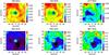 |
Fig. 1 Planck stacked maps at the positions of the final sample of 645 clusters. The maps are 2° × 2° in size and are in units of MJy sr-1. Black contours represent circles with a radius equal to 10′, 30′, and 60′. |
Because the sky fluctuations from the cosmic infrared background (CIB) are stronger than the brightness expected from a single object, we cannot detect the dust contribution to the IR emission from individual clusters of galaxies. However, we can statistically detect the population of clusters by averaging local maps centred at known cluster positions, thereby reducing the background fluctuations (see e.g. Montier & Giard 2005; Giard et al. 2008). Here we take advantage of the “IAS stacking library” (Bavouzet et al. 2008; Béthermin et al. 2010) in order to co-add cluster-centred regions and increase the statistical significance of the IR signal at each frequency. Patches of 2° × 2°, centred on the cluster positions (using 2′ pixels) have been extracted for the six Planck-HFI frequency channels, as well as for the 100 and 60-μm IRIS maps. To ensure a high signal-to-noise ratio and low level of contamination, the low reliability (“category 3”) PSZ1 cluster candidates (126 objects out of 1227) have been excluded from the analysis.
We now detail the different steps of the stacking approach that we adopt to perform our analysis. This includes extraction of the maps at each frequency, foreground removal, and selection of the final cluster sample.
3.1. Field selection
3.1.1. Exclusion of CO contaminated regions
The 100, 217, and 353-GHz Planck channels can be significantly contaminated by the signal due to the emission of CO rotational transition lines at 115, 230, and 345 GHz, respectively (Planck Collaboration IX 2014). Component separation methods have been used to reconstruct CO maps from Planck data (Planck Collaboration et al. 2014). Since the CO emission can be an important foreground for the purpose of the present work, we choose to use a quite strict CO mask. This mask is based on the released CO J = 1 → 0Planck map (Planck Collaboration et al. 2014) and it has been obtained by applying a 3 KRJ km s-1 cut on the CO map (where the KRJ unit comes from intensity scaled to temperature using the Rayleigh-Jeans approximation). We conservatively exclude from the stacking procedure all the fields in which we find flagged pixels, according to the CO mask, at cluster-centric distances ≤1°. This leads to the exclusion of 55 extra clusters, living us with 1046 remaining clusters.
3.1.2. Point source mask
Before proceeding to stack the cluster-centred fields, we check that they are characterized by comparable background contributions. As a first step we verify the presence of known point sources, using the masks provided by the Planck Collaboration for the six frequencies considered here, as well as the IRAS point source catalogue (Helou & Walker 1988). We exclude all fields in which point sources are found at cluster-centric distances ≤5′, even if this is the case only for a single channel. For point sources at larger distances from the nominal cluster position we set the corresponding pixel values to the mean for the pixels within the  region of the 2° × 2° patch, at each wavelength. We also check that all the selected cluster fields have a variance in the region that is ≤5 times that of the whole sample. These additional cuts lead to a reduced sample of 645 clusters, with only two clusters lying at Galactic latitudes lower than 10°. We have also tested the more conservative choice of excluding all the fields in which known point sources are found at ≤10′ from the centre. This substantially reduces the sample size (to 504 clusters), while giving no significant difference in the recovered signal, as will be discussed later.
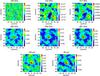 |
Fig. 2 Background- and foreground-cleaned stacked maps, for the final sample of 645 clusters. The units here are MJy sr-1. The extent of the stacked y-signal is represented by black contours for regions of 0.5, 0.1, and 0 times the maximum of the signal (in solid, dashed, and dot-dashed lines, respectively). See Sect. 3.2 for further details. |
3.2. Stacking of the selected fields
We give the same weight to all the cluster fields, since having a particular cluster dominate the average signal is not useful for the purposes of examining the properties of the whole population. The choice of using a constant patch size is motivated by the fact that the differences in cluster angular sizes are negligible when dealing with a 10′ resolution map. Even if a few tens of very low-z clusters (say z< 0.1) are present within the final sample, the average typical size of the sample clusters ( , with a median of 5.́7) allows us to integrate the total flux in the stacked maps within a fixed radius, which we choose to be 15′. The suitability of this choice is verified by looking at the integrated signal as a function of aperture radius.
In Fig. 1 we show the stacked 2° × 2° patches, for the Planck-HFI frequencies. Since no foreground or offset removal has been performed the dust signature is not easily apparent, but instead we can see the negative tSZ signal dominating at ν ≤ 143 GHz and CMB anisotropies at 217 GHz, with the dust contribution becoming stronger at ν ≥ 353 GHz. We also stack the CMB and tSZ maps (Sect. 2.1.2), i.e.  and
and  , summing over all the selected clusters i. These two quantities are then subtracted from the raw frequency maps (
 shown in Fig. 1), specifically calculating
  , where ftSZ,ν is the conversion factor from the tSZ Compton parameter y to MJy sr-1 for each frequency ν. Following Giard et al. (2008), we then perform a background-subtraction procedure by fitting a 3rd-order polynomial surface to the map region for which the cluster-centric distance is above 10′. Finally we also subtract the average signal found for pixels with a distance from the centre that lies between 0.̊5 and 1°, which is used to compute the zero level of the map.
The cleaned and stacked maps are shown in Fig. 2. The same results are obtained if foregrounds and offsets are subtracted cluster by cluster or if we directly stack the cleaned cluster-centred patches. Although we already have hints of a signal at the centre of 143 GHz map, the detection of a significant central positive peak starts at 217 GHz, and is very clearly observed at ν ≥ 353 GHz. Between 100 and 217 GHz the signal is expected to be fainter, according to the typical SED of thermal dust emission. The black contours in Fig. 2 allow comparison with the distribution of the cluster hot gas, representing where the stacked y-map has a value that is 0.5, 0.1, and 0 times its maximum. As expected, the recovered IR emission follows the distribution of the main cluster baryonic component, and thus the extent of the clusters. The average intensity profiles as a function of radius are also provided in Fig. A.1.
Since IR dust emission cannot be detected for individual clusters, average values have been obtained, and the associated uncertainties determined using a bootstrap approach. This consists of constructing and stacking many (300) cluster samples obtained by randomly replacing sources from the original sample, so that each of them contains the same number of clusters as the initial one. The statistical properties of the population being stacked can be then determined by looking at the mean and standard deviation of the flux found in the stacked maps corresponding to each of the resampled cluster lists. We checked that the average values obtained with this resampling technique are equal to what we obtained directly on the original stacked map (without any resampling). This is important, since it indicates that we are indeed stacking a homogeneous population of objects, and that the detected signal is not due to only a small number of a clusters. The mean values recovered are also consistent with the expectations described in Montier & Giard (2005), given the redshift distribution of the sample considered here.
In Table 1 we report, for each frequency: the average fluxes, F, found when integrating out to 15′ from the centre; the standard deviation found using the bootstrap resampling, ΔFb; and an estimate of the uncertainty on the flux at each frequency, ΔF. The flux uncertainties, ΔF, have been obtained as the standard deviation of the fluxes found at random positions in a 2° × 2° region, located further than 15′ from the centre, both using the cluster-centred stacked maps and the “depointed” stacked maps (discussed in Sect. 3.3).
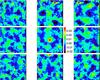 |
Fig. 3 Tests of stacking on “depointed” regions. The central panel shows the stacked result obtained at 857 GHz for the 645 cluster-centred patches (as in Fig. 2). This is surrounded by the eight neighboring maps obtained by changing the cluster Galactic longitude or latitude (or both) by ± 1°. |
3.3. Robustness tests
In order to test the robustness of our results, we have performed various checks, following an approach similar to that of Montier & Giard (2005). Figure 3 shows the 2° × 2° depointed maps that we obtain at 857 GHz when we repeat the same stacking procedure by changing the cluster Galactic longitudes and/or latitudes by ± 1°. This has been done for all the frequency channels and shows that the detection is not an artefact of the adopted stacking scheme. The mean of the fluxes obtained at the centre of the depointed regions is consistent with zero within the uncertainties (i.e. ΔF).
The approach adopted to derive the uncertainty on the flux ΔF has also been applied to a random sample of positions on the sky, whose Galactic latitude distribution follows that of the real clusters in our sample. The derived uncertainties, ΔFran, are listed in Table 1. As for the depointed regions, the mean fluxes obtained at the centre of the random patches are consistent with zero, within the given uncertainties. The values obtained for ΔFran are systematically higher than ΔF. This was to be expected, since Planck blind tSZ detections are more likely in regions that are cleaner of dust contamination. For different cuts in Galactic latitude, moving away from the Galactic plane, ΔFran decreases. This might indicate that some residual contamination due to Galactic dust emission is present. Indeed, in Fig. 2 we can see a correlation between frequencies for the residual fluctuations in the region surrounding the clusters. Such a correlation between frequencies could be also introduced by the process of subtracting the contamination maps (CMB and tSZ), since these are built from the same Planck-HFI maps. However the CMB anisotropies and the tSZ signal are both negligible at ν ≥ 545 GHz. The uncertainty ΔFran is of the order of ΔFb and ΔF at the frequencies for which we have a significant detection; hence this contribution does not dominate the signal and we can consider it to be accounted for in the error budget. For this reason, we do not impose any extra selection cut in Galactic latitude in order to maximize the sample size.
As a further cross-check, we have tested the robustness of the results by alternatively adding and subtracting the patches centred at the cluster positions. This approach shows that none of the individual patches dominates the final average signal, in agreement with the results of the bootstrap resampling procedure.
Fluxes found in the co-added maps for a sample of 645 clusters extracted from the first Planck Catalogue of SZ sources.
4. SED of the cluster IR emission
4.1. SED model
Using the cleaned stacked maps obtained in Sect. 3, we derive the IR fluxes for each of the frequencies considered. In Fig. 4 we show the average SED of galaxy clusters from 60μm to 3 mm (as listed in Table 1).
The SED shown in Fig. 4 behaves like Galactic dust, confirming the hypothesis of thermal dust emission. It can be well represented by modified blackbody emission (the black curve in Fig. 4), with spectral index β. This accounts for the fact that the IR emission from clusters is not a perfect blackbody, but has a power-law dust emissivity κν = κ0(ν/ν0)β, i.e. 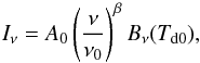 (1)where β is the emissivity index, Bν is the Planck function, Td0 the dust temperature, and A0 an overall amplitude. The combination of Planck and IRAS spectral coverage allows us to sample the SED of the average IR cluster across its emission peak. The reconstructed SED can be used to constrain the dust temperature and also the amplitude A0, which is directly related to the dust mass. Following the prescription of Hildebrand (1983), the dust mass can be in fact estimated from the observed flux densities and the modified blackbody temperature as
  (2)with the “K-correction” being
  (3)which allows translation to monochromatic rest-frame flux densities, Sν. Here νobs represents the observed frequency and νem the rest-frame frequency, with νobs = νem/ (1 + z), and D is the radial comoving distance. The amplitude parameter A0 then provides an estimate of the overall dust mass:
  (4)provided we know κν0, the dust opacity at a given frequency ν0, with Ω being the solid angle. Here we adopt the value κ850 = 0.0383 m2 kg-1 (Draine 2003).
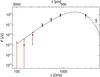 |
Fig. 4 Average SED for galaxy clusters. In black points we show the flux, as a function of frequency, found in the co-added maps obtained for a sample of 645 clusters. The error bars in black correspond to the dispersion estimated using bootstrap resampling (ΔFb, Table 1). The red error bars have been estimated as the standard deviation of the flux integrated at random positions away from each cluster region (ΔF, Table 1). The black solid line shows the best-fit modified blackbody model (with β = 1.5). We note that the highest frequency point (60 μm from IRAS) is not used in the fit. |
For the different cluster samples considered here: average redshifts (z), characteristic radii (θ500) and total masses at a radius for which the mean cluster density is 500 and 200 times the critical density of the Universe ( and
and  ).
).
This model has the advantage of being accurate enough to adequately fit the data, while providing a simple interpretation of the observations, with a small number of parameters. Even though studies of star-forming galaxies have demonstrated the inadequacy of a single temperature model for detailed, high signal-to-noise SED shapes (e.g. Dale & Helou 2002; Wiklind 2003), the cold dust component (λ ≳ 100 μm) tends to be well represented using a single effective temperature modified blackbody (Draine & Li 2007; Casey 2012; Clemens et al. 2013). Figure 4 shows that a further component would indeed permit us to also fit the 60μm point (the rightmost point in Fig. 4). This excess at high frequency could be caused by smaller grains that are not in thermal equilibrium with the radiation field; they are stochastically heated and therefore their emission is not a simple modified blackbody (Compiègne et al. 2011; Jones et al. 2013). However, this additional contribution would be sub-dominant at λ ≥ 100 μm and so would not significantly change the derived temperature and mass of the cold dust, which corresponds to the bulk of the dust mass in galaxies (Cortese et al. 2012; Davies et al. 2012; Santini et al. 2014). We choose then to adopt a single-component approach and exclude the 60μm from the data used for the fit. Not doing this would bias the estimate of the temperature and mass of the cold dust.
In Planck Collaboration Int. XXII (2015) the Planck-HFI intensity (and polarization) maps were used to estimate the spectral index β of the Galactic dust emission. On the basis of nominal mission data, they found that, at ν< 353 GHz, the dust emission can be well represented by a modified blackbody spectrum with β = 1.51 ± 0.06. At higher frequencies (100 μm−353 GHz) β = 1.65 was assumed. In the following we have adopted a single spectral index over the whole spectral range, and β = 1.5 will be our baseline value. In some other studies an emissivity index β = 2 has been used instead, for example in the analysis of Davies et al. (2012), which focused on Herschel data (at 100−500μm) to explore the IR properties of cluster galaxies (specifically 78 galaxies in the Virgo cluster).
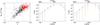 |
Fig. 5 SEDs for cluster sub-samples. Left: in the redshift−mass plane, we show the distribution of the 561 Planck clusters with known redshift, which are used in this paper. Different colours (black and red) are used for the low- and high-redshift sub-samples, while different symbols (dots and diamonds) are used for the low- and high-mass sub-samples. Middle: in blue circles the 254 clusters at z> 0.25 and in orange triangles the 307 clusters at z ≤ 0.25 (307 clusters), plotted along with the corresponding best-fit models (dashed and dash-dotted lines, respectively). Left: in blue the 241 clusters with Mtot> 5.5 × 10¹⁴M⊙ and in orange the 320 clusters with Mtot ≤ 5.5 × 10¹⁴M⊙, along with the best-fit models (dashed and dash-dotted lines, respectively). The rightmost (IRAS) point is not used in the fit. |
4.2. Dust temperature and mass
By representing the recovered SEDs with a single-temperature modified blackbody dust model and fixing β, we can constrain the SED and estimate the average dust temperature. This is for the observer’s frame, while the temperature in the rest-frame of the cluster will be given by Td = Td0(1 + z).
We use a χ2 minimization approach and account for colour corrections when comparing the measured SED to the modelled one. In Table 2 (upper line) we report the best-fit values that we obtain for Td0 and Mdust4 when considering the sample of 645 clusters, as well as the two redshift and mass sub-samples. The associated uncertainties are derived from the statistical ones obtained through the χ2 minimization in the fitting procedure (with ΔFb being the error on the flux at each frequency). The corresponding uncertainties on the dust mass estimates have been derived using random realizations of the model, letting Td0 and A0 vary within the associated uncertainties and accounting for the correlation between the two. The best-fit models (β = 1.5) is represented in Figs. 4 by the black solid line. For the whole sample of 645 objects, we assume that the mean redshift is the mean of the known redshifts (z = 0.26 ± 0.17). We then obtain Td = (24.2 ± 3.0 ± 2.8) K, where the additional systematic uncertainty is due to the redshift dispersion of our sample (see the second column of Table 2), and an average dust mass of (1.08 ± 0.32) × 1010M⊙.
The recovered dust temperatures are in agreement with those observed for the dust content in various field galaxy samples (e.g. Dunne et al. 2011; Clemens et al. 2013; Symeonidis et al. 2013) and with the values expected for the cold dust component in cluster galaxies, e.g. the Virgo sample explored by Davies et al. (2012) and di Serego Alighieri et al. (2013). Our dust mass estimates are similar to those obtained with different approaches by Muller et al. (2008; Md = 8 × 10⁹M⊙) for a sample with a comparable redshift distribution and Gutiérrez & López-Corredoira (2014; Md< 8.4 × 10⁹M⊙) for a relatively low-mass cluster sample.
4.2.1. Additional sources of uncertainties and residual contamination
The spectral index β is known to vary with environment. Shown by Planck to be equal to 1.50 for the diffuse ISM in the Solar neighbourhood, β is known to be higher in molecular clouds (Planck Collaboration XI 2014). This reflects variations in the composition and structure of dust, something which is clearly seen in laboratory measurements (e.g. Jones et al. 2013). The impact of the adopted emissivity index on our results is explored by varying its value between 1.3 and 2.2. For the total sample of 645 clusters, we have explored how this affects Td0 and Mdust, and we summarize the results in Table 2. When we compare the dust temperature obtained with the same choice of β, i.e. β = 2, the dust temperatures that we find are similar to those obtained by Davies et al. (2012) for the galaxies of the Virgo cluster. The range explored shows that when reducing β the inferred T0 increases, and vice versa, as expected given the degeneracy between these two parameters (e.g. Sajina et al. 2006; Désert et al. 2008; Kelly et al. 2012; Planck Collaboration Int. XIV 2014). However, the differences are not significant within the associated uncertainties, reflecting the fact that our data are not good enough to simultaneously constrain the temperature, the amplitude, and also the spectral index. Different values of β can affect the dust mass estimates by up to 20%, which is however negligible with respect to the existing uncertainty on the dust opacity κν.
Figure 4 shows that the 143 and 353 GHz intensities are slightly lower and higher, respectively, with respect to the best-fit model. This might indicate a residual tSZ contamination, since the tSZ signal is negative at 143 GHz and positive at 353 GHz. The SZ amplitude that we subtract has been estimated under the non-relativistic hypothesis, and this could result in a slight underestimation of the cluster Comptonization parameter y. Although the relativistic correction is expected to have a small impact on the inferred Compton parameter, we should note that for cluster temperatures of a few Kelvin the relativistic correction boosts the tSZ flux at 857 by a factor of several tens of a percent. Given the amplitude of the SZ contribution at this frequency with respect to the dust emission, this contribution remains negligible. On the other hand, the cluster IR component we are considering here is not included in none of the simulations used to test the MILCA algorithm and might bias somehow the reconstruction of the tSZ amplitude. Then we have verified that the residual tSZ contamination is negligible by fitting, a posteriori, the dust SED as a linear combination of the modified blackbody and a tSZ contribution. For the two components we find an amplitude consistent with 1 and 0, respectively.
The normalization of the dust opacity represents the major source of uncertainty in deriving dust masses from observed IR fluxes (Fanciullo et al. 2015). The Draine (2003) value of κ850 was derived from a dust model (including assumptions about chemical composition, distribution of grain size, etc.) that shows good agreement with available data. However, using a different approach, James et al. (2002) found κ850 = (0.07 ± 0.02) m2 kg-1, nearly a factor of 2 higher. The latter value uses a calibration that has been obtained with a sample of galaxies for which the IR fluxes, gas masses, and metallicities are all available, and adopts the assumption that the fraction of metals bound up in dust is constant for all the galaxies in the sample. Planck Collaboration Int. XXIX (2016) has shown that the opacity of the Draine (2003) model needs to be increased by a factor of 1.8 to fit the Planck data, as well as extinction measurements, and this moves the normalization towards the value suggested by James et al. (2002).
4.2.2. Possible evolution with mass and redshift
As a first attempt to investigate how clusters of different mass and at different redshift contribute to the overall average signal, we have divided our sample into two different sub-samples, according to their redshifts and their masses. An increased IR emission with redshift was in fact seen in Planck Collaboration XXIII (2016; for z < 0.15 versus z > 0.15), in which a similar stacking was performed on Planck data to investigate the cross-correlation between the tSZ effect and the CIB fluctuations. This is expected since in more distant (younger) clusters there will be more gas-rich active (i.e. star-forming) spirals. Conversely, nearby clusters mainly contain elliptical galaxies, with a lower star-formation rate and little dust. But we also expect the overall IR signal to be higher for higher mass objects. We expect dust emission to be proportional to the total cluster mass because they should both be tightly correlated with the number of galaxies (Giard et al. 2008; da Silva et al. 2009).
We have considered clusters above and below z = 0.25 (with 254 and 307 sources, respectively) and above and below  (241 and 320 sources, respectively)5. The left panel in Fig. 5 provides the z−Mtot distribution of the 561 Planck clusters with known redshift used in this paper. This figure shows that the two partitions do not trace exactly the same populations, but they are also not completely independent. The lower redshift bin strongly overlaps with lower mass systems and vice versa. The middle and right panels show the measured SED for the low (orange) and high (blue) redshift and mass sub-samples, respectively.
For the low-redshift and low-mass sub-samples we have no detection at ν < 353 GHz (Fig. 5, middle panel). The SEDs for the two redshift sub-samples are consistent with each other (within ΔFb), even though fluxes are systematically higher at higher z. For the high- and low-mass sub-samples, the difference between the two SEDs becomes more important, with higher fluxes when  (Fig. 5, right panel). A similar behaviour for the sub-samples in and z is not surprising, given the correlation between the two (Fig. 5, left panel).
In Table 2 we list the best fit parameters obtained for the four sub-samples. We observe a slight increase of dust temperature with mass and redshift, but no significant evolution within the uncertainties. On the other side, for the low- and high-mass sub-samples we find significantly different values of the overall dust mass, implying that the dust mass is responsible for the difference between the two curves in the middle panel of Fig. 5 and that the evolution we observe, also in z, is manly due to the correlation between Md and Mtot.
4.3. Dust-to-gas mass ratio
We now estimate the ratio of dust mass to gas mass, Zd, directly from the observed IR cluster signal. To do so we need an estimate of the cluster gas mass. The IR fluxes used in the previous section to estimate Md were obtained by integrating the signal out to 15′ from the cluster centres, without any rescaling of the maps with respect to each cluster’s characteristic radius. In the PSZ1, the mass information is provided at θ500, and for our sample this size is significantly smaller than 15′ for almost all clusters (see Table 2). However, we can take advantage of the self-similarity of cluster profiles, from which it follows that the ratio between radii corresponding to different overdensities is nearly constant over the cluster population. Therefore we will use θ200 and assume that θ200 ≃ 1.4 × θ500 (Ettori & Balestra 2009) to obtain the corresponding enclosed total mass  . Here, θ500 is obtained from the values listed in the PSZ1. The cluster total mass also provides an estimate of the gas mass,
  (e.g. Pratt et al. 2009; Comis et al. 2011; Planck Collaboration Int. V 2013; Sembolini et al. 2013). Assuming that Md and correspond to comparable cluster regions, we find that Zd = (1.93 ± 0.92) × 10-4 for the full sample. For the low- and high-redshift sub-samples we find (0.79 ± 0.50) × 10-4 and (3.7 ± 1.5) × 10-4, respectively, while for the low- and high-mass sub-samples we obtain (0.51 ± 0.37) × 10-4 and (4.6 ± 1.5) × 10-4, respectively. We note that the uncertainties quoted here do not account for the fact that the gas fraction might vary from cluster to cluster, and as a function of radius/mass and redshift.
These dust-to-mass ratios are derived from the overall IR flux, which is the sum of the contribution due to the cluster galaxies and a possible further contribution coming from the ICM dust component. Therefore they represent an upper limit for the dust fraction that is contained within the IGM/ICM. These values are consistent with the upper limit (5 × 10⁻⁴) derived by Giard et al. (2008) from the LIR/LX ratio and a model for the ICM dust emission (Montier & Giard 2004).
5. Conclusions
We have adopted a stacking approach in order to recover for the first time, the average SED of the IR emission towards galaxy clusters. Considering the Catalogue of Planck SZ Clusters, we have used the Planck-HFI maps (from 100 to 857 GHz) and the IRAS maps (IRIS data at 100 and 60μm) in order to sample the SED of the cluster dust emission on both sides of the expected emissivity peak.
For a sample of 645 clusters selected from the PSZ1 catalogue, we find significant detection of dust emission from 353 to 857 GHz, and at 100μm and 60μm, at the cluster positions, after cleaning for foreground contributions. By co-adding maps extracted at random positions on the sky, we have verified that the residual Galactic emission is accounted for in the uncertainty budget. For the IRAS frequencies, we find average central intensities that are in agreement with the values found by Montier & Giard (2005). The measured SED is consistent with dust IR emission following a modified blackbody distribution.
These results have allowed us to constrain, directly from its IR emission, both the average overall dust temperature and the dust mass in clusters. From the average cluster SED of a total sample of 645 clusters, we infer an average dust temperature of Td = (24.2 ± 3.0) K, in agreement with what is observed for galaxy thermal dust emission and an average dust mass of Md = (1.25 ± 0.37) × 1010M⊙. By dividing our initial sample into two bins, according to either their mass or redshift, we find that the IR emission is larger for the higher mass (or higher redshift) clusters. This difference is mainly due to the positive correlation between dust mass and cluster total mass, the resulting IR emission being proportional to the latter. Our sample is not ideal for taking the next step and constraining the mass and redshift evolution of the IR emission of the cluster dust component because it is not complete and we do not dispose of a well-characterized selection function for it. Furthermore, the redshift and mass bins, although they do not trace exactly the same cluster population, are not independent either. With a larger sample, and a wider distribution in mass and redshift, the separate mass and redshift dependance could be studied much more thoroughly, for example by correlating the weak signals from individual clusters with Mtot and z. This approach would allow us to better account for different distances, masses, and selection effects.
Using the total mass estimates for each cluster, we also derive the average cluster dust-to-gas mass ratio Zd = (1.93 ± 0.92) × 10-4. This leads to an upper limit on the dust fraction within the ICM that is consistent with previous results. Most of the IR signal detected in the maps stacked at cluster positions was expected to be due to the contribution of the member galaxies (e.g. Roncarelli et al. 2010). And the recovered temperature, typical of values found in the discs of galaxies, is in agreement with this. However, if we also take into account the additional uncertainties on the dust mass estimates coming from the spectral index and the dust opacity (up to 20% and 50%, respectively), our results cannot exclude a dust fraction that, according to Montier & Giard 2004, would imply that the IR ICM dust emission is an important factor in the cooling of the intra-cluster gas.
Planck (http://www.esa.int/Planck) is a project of the European Space Agency (ESA) with instruments provided by two scientific consortia funded by ESA member states and led by Principal Investigators from France and Italy, telescope reflectors provided through a collaboration between ESA and a scientific consortium led and funded by Denmark, and additional contributions from NASA (USA).
We report Mdust rather than A0, the overall amplitude to which it is proportional, see Sect. 4.2.
is the total mass contained within a radius (θ500) at which the mean cluster density is 500 times the critical density of the Universe.
Acknowledgments
The Planck Collaboration acknowledges the support of: ESA; CNES, and CNRS/INSU-IN2P3-INP (France); ASI, CNR, and INAF (Italy); NASA and DoE (USA); STFC and UKSA (UK); CSIC, MINECO, JA, and RES (Spain); Tekes, AoF, and CSC (Finland); DLR and MPG (Germany); CSA (Canada); DTU Space (Denmark); SER/SSO (Switzerland); RCN (Norway); SFI (Ireland); FCT/MCTES (Portugal); ERC and PRACE (EU). A description of the Planck Collaboration and a list of its members, indicating which technical or scientific activities they have been involved in, can be found at http://www.cosmos.esa.int/web/planck/planck-collaboration. This paper makes use of the HEALPix software package. We acknowledge the support of grant ANR-11-BS56-015. We are thankful to the anonymous referee for useful comments that helped improve the quality of the paper.
References
- Bavouzet, N., Dole, H., Le Floc’h, E., et al. 2008, A&A, 479, 83 [NASA ADS] [CrossRef] [EDP Sciences] [Google Scholar]
- Béthermin, M., Dole, H., Beelen, A., & Aussel, H. 2010, A&A, 512, A78 [NASA ADS] [CrossRef] [EDP Sciences] [Google Scholar]
- Braglia, F. G., Ade, P. A. R., Bock, J. J., et al. 2011, MNRAS, 412, 1187 [NASA ADS] [Google Scholar]
- Casey, C. M. 2012, MNRAS, 425, 3094 [Google Scholar]
- Chelouche, D., Koester, B. P., & Bowen, D. V. 2007, ApJ, 671, L97 [NASA ADS] [CrossRef] [Google Scholar]
- Clemens, M. S., Negrello, M., De Zotti, G., et al. 2013, MNRAS, 433, 695 [NASA ADS] [CrossRef] [Google Scholar]
- Comis, B., de Petris, M., Conte, A., Lamagna, L., & de Gregori, S. 2011, MNRAS, 418, 1089 [NASA ADS] [CrossRef] [Google Scholar]
- Compiègne, M., Verstraete, L., Jones, A., et al. 2011, A&A, 525, A103 [NASA ADS] [CrossRef] [EDP Sciences] [Google Scholar]
- Coppin, K. E. K., Geach, J. E., Smail, I., et al. 2011, MNRAS, 416, 680 [NASA ADS] [Google Scholar]
- Cortese, L., Ciesla, L., Boselli, A., et al. 2012, A&A, 540, A52 [NASA ADS] [CrossRef] [EDP Sciences] [Google Scholar]
- da Silva, A. C., Catalano, A., Montier, L., et al. 2009, MNRAS, 396, 849 [NASA ADS] [CrossRef] [Google Scholar]
- Dale, D. A., & Helou, G. 2002, ApJ, 576, 159 [NASA ADS] [CrossRef] [Google Scholar]
- Davies, J. I., Bianchi, S., Cortese, L., et al. 2012, MNRAS, 419, 3505 [NASA ADS] [CrossRef] [Google Scholar]
- Désert, F.-X., Macías-Pérez, J. F., Mayet, F., et al. 2008, A&A, 481, 411 [NASA ADS] [CrossRef] [EDP Sciences] [Google Scholar]
- di Serego Alighieri, S., Bianchi, S., Pappalardo, C., et al. 2013, A&A, 552, A8 [NASA ADS] [CrossRef] [EDP Sciences] [Google Scholar]
- Draine, B. T. 2003, ARA&A, 41, 241 [NASA ADS] [CrossRef] [Google Scholar]
- Draine, B. T., & Li, A. 2007, ApJ, 657, 810 [NASA ADS] [CrossRef] [Google Scholar]
- Dunne, L., Gomez, H. L., da Cunha, E., et al. 2011, MNRAS, 417, 1510 [NASA ADS] [CrossRef] [Google Scholar]
- Dwek, E., & Arendt, R. G. 1992, ARA&A, 30, 11 [NASA ADS] [CrossRef] [Google Scholar]
- Dwek, E., Rephaeli, Y., & Mather, J. C. 1990, ApJ, 350, 104 [NASA ADS] [CrossRef] [Google Scholar]
- Ettori, S., & Balestra, I. 2009, A&A, 496, 343 [NASA ADS] [CrossRef] [EDP Sciences] [Google Scholar]
- Fanciullo, L., Guillet, V., Aniano, G., et al. 2015, A&A, 580, A136 [NASA ADS] [CrossRef] [EDP Sciences] [Google Scholar]
- Giard, M., Montier, L., Pointecouteau, E., & Simmat, E. 2008, A&A, 490, 547 [NASA ADS] [CrossRef] [EDP Sciences] [Google Scholar]
- Gorski, K. M., Wandelt, B. D., Hansen, F. K., Hivon, E., & Banday, A. J. 1999, ArXiv e-print [arXiv:astro-ph/9905275] [Google Scholar]
- Górski, K. M., Hivon, E., Banday, A. J., et al. 2005, ApJ, 622, 759 [NASA ADS] [CrossRef] [Google Scholar]
- Gutiérrez, C. M., & López-Corredoira, M. 2014, A&A, 571, A66 [NASA ADS] [CrossRef] [EDP Sciences] [Google Scholar]
- Helou, G., & Walker, D. W. 1988, Infrared astronomical satellite (IRAS) catalogs and atlases, Volume 7: The small scale structure catalog [Google Scholar]
- Hildebrand, R. H. 1983, Quant. J. Rev. Astron. Soc., 24, 267 [Google Scholar]
- Hurier, G., Macías-Pérez, J. F., & Hildebrandt, S. 2013, A&A, 558, A118 [NASA ADS] [CrossRef] [EDP Sciences] [Google Scholar]
- James, A., Dunne, L., Eales, S., & Edmunds, M. G. 2002, MNRAS, 335, 753 [NASA ADS] [CrossRef] [Google Scholar]
- Jones, A. P., Fanciullo, L., Köhler, M., et al. 2013, A&A, 558, A62 [NASA ADS] [CrossRef] [EDP Sciences] [Google Scholar]
- Kelly, D. M., & Rieke, G. H. 1990, ApJ, 361, 354 [NASA ADS] [CrossRef] [Google Scholar]
- Kelly, B. C., Shetty, R., Stutz, A. M., et al. 2012, ApJ, 752, 55 [NASA ADS] [CrossRef] [Google Scholar]
- Kitayama, T., Ito, Y., Okada, Y., et al. 2009, ApJ, 695, 1191 [NASA ADS] [CrossRef] [Google Scholar]
- Miville-Deschênes, M.-A., & Lagache, G. 2005, ApJS, 157, 302 [NASA ADS] [CrossRef] [Google Scholar]
- Montier, L. A., & Giard, M. 2004, A&A, 417, 401 [NASA ADS] [CrossRef] [EDP Sciences] [Google Scholar]
- Montier, L. A., & Giard, M. 2005, A&A, 439, 35 [NASA ADS] [CrossRef] [EDP Sciences] [Google Scholar]
- Muller, S., Wu, S.-Y., Hsieh, B.-C., et al. 2008, ApJ, 680, 975 [NASA ADS] [CrossRef] [Google Scholar]
- Planck Collaboration IX. 2014, A&A, 571, A9 [NASA ADS] [CrossRef] [EDP Sciences] [Google Scholar]
- Planck Collaboration XI. 2014, A&A, 571, A11 [NASA ADS] [CrossRef] [EDP Sciences] [Google Scholar]
- Planck Collaboration, Ade, P. A. R., Aghanim, N., et al. 2014, A&A, 571, A13 [NASA ADS] [CrossRef] [EDP Sciences] [Google Scholar]
- Planck Collaboration XXI. 2014, A&A, 571, A21 [NASA ADS] [CrossRef] [EDP Sciences] [Google Scholar]
- Planck Collaboration XXIX. 2014, A&A, 571, A29 [NASA ADS] [CrossRef] [EDP Sciences] [Google Scholar]
- Planck Collaboration XXXII 2015, A&A, 581, A14 [NASA ADS] [CrossRef] [EDP Sciences] [Google Scholar]
- Planck Collaboration I. 2016, A&A, 594, A1 [NASA ADS] [CrossRef] [EDP Sciences] [Google Scholar]
- Planck Collaboration XXII. 2016, A&A, 594, A22 [NASA ADS] [CrossRef] [EDP Sciences] [Google Scholar]
- Planck Collaboration XXIII. 2016, A&A, 594, A23 [NASA ADS] [CrossRef] [EDP Sciences] [Google Scholar]
- Planck Collaboration XXVII. 2016, A&A, 594, A27 [NASA ADS] [CrossRef] [EDP Sciences] [Google Scholar]
- Planck Collaboration Int. V. 2013, A&A, 550, A131 [NASA ADS] [CrossRef] [EDP Sciences] [Google Scholar]
- Planck Collaboration Int. XIV. 2014, A&A, 564, A45 [NASA ADS] [CrossRef] [EDP Sciences] [Google Scholar]
- Planck Collaboration Int. XXII. 2015, A&A, 576, A107 [NASA ADS] [CrossRef] [EDP Sciences] [Google Scholar]
- Planck Collaboration Int. XXVI. 2015, A&A, 582, A29 [NASA ADS] [CrossRef] [EDP Sciences] [Google Scholar]
- Planck Collaboration Int. XXIX. 2016, A&A, 586, A132 [NASA ADS] [CrossRef] [EDP Sciences] [Google Scholar]
- Planck Collaboration Int. XXXVI. 2016, A&A, 586, A139 [NASA ADS] [CrossRef] [EDP Sciences] [Google Scholar]
- Popescu, C. C., Tuffs, R. J., Fischera, J., & Völk, H. 2000, A&A, 354, 480 [NASA ADS] [Google Scholar]
- Pratt, G. W., Croston, J. H., Arnaud, M., & Böhringer, H. 2009, A&A, 498, 361 [NASA ADS] [CrossRef] [EDP Sciences] [Google Scholar]
- Roncarelli, M., Pointecouteau, E., Giard, M., Montier, L., & Pello, R. 2010, A&A, 512, A20 [NASA ADS] [CrossRef] [EDP Sciences] [Google Scholar]
- Sajina, A., Scott, D., Dennefeld, M., et al. 2006, MNRAS, 369, 939 [NASA ADS] [CrossRef] [Google Scholar]
- Santini, P., Maiolino, R., Magnelli, B., et al. 2014, A&A, 562, A30 [NASA ADS] [CrossRef] [EDP Sciences] [Google Scholar]
- Sarazin, C. L. 1986, Rev. Mod. Phys., 58, 1 [NASA ADS] [CrossRef] [Google Scholar]
- Sarazin, C. L. 1988, X-ray emission from clusters of galaxies (Campridge University Press) [Google Scholar]
- Sembolini, F., Yepes, G., De Petris, M., et al. 2013, MNRAS, 429, 323 [NASA ADS] [CrossRef] [Google Scholar]
- Stickel, M., Klaas, U., Lemke, D., & Mattila, K. 2002, A&A, 383, 367 [NASA ADS] [CrossRef] [EDP Sciences] [Google Scholar]
- Sunyaev, R. A., & Zeldovich, Y. B. 1972, Comm. Astrophys. Space Phys., 4, 173 [Google Scholar]
- Sunyaev, R. A., & Zeldovich, I. B. 1980, ARA&A, 18, 537 [NASA ADS] [CrossRef] [Google Scholar]
- Symeonidis, M., Vaccari, M., Berta, S., et al. 2013, MNRAS, 431, 2317 [NASA ADS] [CrossRef] [Google Scholar]
- Weingartner, J. C., Draine, B. T., & Barr, D. K. 2006, ApJ, 645, 1188 [NASA ADS] [CrossRef] [Google Scholar]
- Welikala, N., Béthermin, M., Guery, D., et al. 2016, MNRAS, 455, 1629 [NASA ADS] [CrossRef] [Google Scholar]
- Wiklind, T. 2003, ApJ, 588, 736 [NASA ADS] [CrossRef] [Google Scholar]
Appendix A: Additional figure
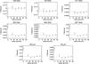 |
Fig. A.1 Radial profiles obtained from the background- and foreground-cleaned stacked maps, for the sample of 645 clusters. The units here are MJy sr-1. The black points correspond to the values obtained as the average of the pixels contained within each region considered and associated uncertainties have been obtained using bootstrap resampling. We find no significant detection at 100 and 143 GHz, while the detection starts to become strong at ν ≥ 353 GHz, consistent with what we saw in Fig. 2. |
All Tables
Fluxes found in the co-added maps for a sample of 645 clusters extracted from the first Planck Catalogue of SZ sources.
For the different cluster samples considered here: average redshifts (z), characteristic radii (θ500) and total masses at a radius for which the mean cluster density is 500 and 200 times the critical density of the Universe ( and ).
All Figures
|
Fig. 1 Planck stacked maps at the positions of the final sample of 645 clusters. The maps are 2° × 2° in size and are in units of MJy sr-1. Black contours represent circles with a radius equal to 10′, 30′, and 60′. |
| In the text | |
|
Fig. 2 Background- and foreground-cleaned stacked maps, for the final sample of 645 clusters. The units here are MJy sr-1. The extent of the stacked y-signal is represented by black contours for regions of 0.5, 0.1, and 0 times the maximum of the signal (in solid, dashed, and dot-dashed lines, respectively). See Sect. 3.2 for further details. |
| In the text | |
|
Fig. 3 Tests of stacking on “depointed” regions. The central panel shows the stacked result obtained at 857 GHz for the 645 cluster-centred patches (as in Fig. 2). This is surrounded by the eight neighboring maps obtained by changing the cluster Galactic longitude or latitude (or both) by ± 1°. |
| In the text | |
|
Fig. 4 Average SED for galaxy clusters. In black points we show the flux, as a function of frequency, found in the co-added maps obtained for a sample of 645 clusters. The error bars in black correspond to the dispersion estimated using bootstrap resampling (ΔFb, Table 1). The red error bars have been estimated as the standard deviation of the flux integrated at random positions away from each cluster region (ΔF, Table 1). The black solid line shows the best-fit modified blackbody model (with β = 1.5). We note that the highest frequency point (60 μm from IRAS) is not used in the fit. |
| In the text | |
|
Fig. 5 SEDs for cluster sub-samples. Left: in the redshift−mass plane, we show the distribution of the 561 Planck clusters with known redshift, which are used in this paper. Different colours (black and red) are used for the low- and high-redshift sub-samples, while different symbols (dots and diamonds) are used for the low- and high-mass sub-samples. Middle: in blue circles the 254 clusters at z> 0.25 and in orange triangles the 307 clusters at z ≤ 0.25 (307 clusters), plotted along with the corresponding best-fit models (dashed and dash-dotted lines, respectively). Left: in blue the 241 clusters with Mtot> 5.5 × 10¹⁴M⊙ and in orange the 320 clusters with Mtot ≤ 5.5 × 10¹⁴M⊙, along with the best-fit models (dashed and dash-dotted lines, respectively). The rightmost (IRAS) point is not used in the fit. |
| In the text | |
|
Fig. A.1 Radial profiles obtained from the background- and foreground-cleaned stacked maps, for the sample of 645 clusters. The units here are MJy sr-1. The black points correspond to the values obtained as the average of the pixels contained within each region considered and associated uncertainties have been obtained using bootstrap resampling. We find no significant detection at 100 and 143 GHz, while the detection starts to become strong at ν ≥ 353 GHz, consistent with what we saw in Fig. 2. |
| In the text | |
Current usage metrics show cumulative count of Article Views (full-text article views including HTML views, PDF and ePub downloads, according to the available data) and Abstracts Views on Vision4Press platform.
Data correspond to usage on the plateform after 2015. The current usage metrics is available 48-96 hours after online publication and is updated daily on week days.
Initial download of the metrics may take a while.