| Issue |
A&A
Volume 593, September 2016
|
|
|---|---|---|
| Article Number | A71 | |
| Number of page(s) | 25 | |
| Section | Numerical methods and codes | |
| DOI | https://doi.org/10.1051/0004-6361/201628122 | |
| Published online | 23 September 2016 | |
Uncertainties and biases of source masses derived from fits of integrated fluxes or image intensities
Laboratoire AIM Paris–Saclay, CEA/DSM–CNRS–Université Paris Diderot, IRFU, Service d’Astrophysique, Centre d’Études de Saclay, Orme des Merisiers, 91191 Gif-sur-Yvette, France
e-mail: alexander.menshchikov@cea.fr
Received: 13 January 2016
Accepted: 12 June 2016
Fitting spectral distributions of total fluxes or image intensities are two standard methods for estimating the masses of starless cores and protostellar envelopes. These mass estimates, which are the main source and basis of our knowledge of the origin and evolution of self-gravitating cores and protostars, are uncertain. It is important to clearly understand sources of statistical and systematic errors stemming from the methods and minimize the errors. In this model-based study, a grid of radiative transfer models of starless cores and protostellar envelopes was computed and their total fluxes and image intensities were fitted to derive the model masses. To investigate intrinsic effects related to the physical objects, all observational complications were explicitly ignored. Known true values of the numerical models allow assessment of the qualities of the methods and fitting models, as well as the effects of nonuniform temperatures, far-infrared opacity slope, selected subsets of wavelengths, background subtraction, and angular resolutions. The method of fitting intensities gives more accurate masses for more resolved objects than the method of fitting fluxes. With the latter, a fitting model that assumes optically thin emission gives much better results than the one allowing substantial optical depths. Temperature excesses within the objects above the mass-averaged values skew their spectral shapes towards shorter wavelengths, leading to masses underestimated typically by factors 2−5. With a fixed opacity slope deviating from the true value by a factor of 1.2, masses are inaccurate within a factor of 2. The most accurate masses are estimated by fitting just two or three of the longest wavelength measurements. Conventional algorithm of background subtraction is a likely source of large systematic errors. The absolute values of masses of the unresolved or poorly resolved objects in star-forming regions are uncertain to within at least a factor of 2−3.
Key words: stars: formation / infrared: ISM / submillimeter: ISM / methods: data analysis / techniques: image processing / techniques: photometric
© ESO, 2016
1. Introduction
Significant technological advances in the astronomical instrumentation during the last four decades enabled measurements of the far-infrared thermal dust emission (usually optically thin in that wavelength range) and hence estimates of the masses of dusty objects. Fitting the far-infrared and submillimeter flux or intensity distributions of optically thin sources can give their average temperatures and masses (Hildebrand 1983). This simple method has become standard in studies of Galactic star formation and a major source of our knowledge of the physical properties and evolution of self-gravitating cores and protostars. Although there are more sophisticated approaches (e.g., Kelly et al. 2012), a simple fitting of the observed spectral shapes remains the most widely used method in the observational studies of star formation (e.g., Könyves et al. 2015). Its inaccuracies, biases, and limitations need to be carefully investigated before reliable conclusions can be made on the physical properties and evolution of the observed objects.
Mass derivation from fitting total fluxes or pixel intensities involves a strong assumption of a constant temperature within an object. In addition to such poorly known parameters as the distance, the far-infrared opacity and its power-law slope, and the dust-to-gas mass ratio, the most problematic assumption is that a single color temperature obtained from the fitting is a good approximation of the mass-averaged physical dust temperatures. This may be true for only the simplest case of the lowest density starless cores, transparent in the visible wavelength range and thus practically isothermal, but it is clearly invalid for the protostellar envelopes that are centrally heated by accretion luminosity. Very sensitive dependence of the emission of dust grains on their temperature warrants careful investigation of the effects of nonuniform temperatures. There are papers that have investigated some aspects of the problem, notably the correlation between the estimated temperatures and power-law opacity slopes (e.g., Shetty et al. 2009a,b; Juvela & Ysard 2012, and references therein) and the inaccuracies of mass derivation and their effect on the resulting core mass function (Malinen et al. 2011).
The present purely model-based study simplifies the problem by removing the “observational layer” between the physical reality and observers. To investigate the intrinsic effects related to the physical objects, all observational intricacies (the complex filamentary backgrounds, instrumental noise, calibration errors, different angular resolutions across wavebands, etc.) were explicitly ignored. Measurement errors in intensities and fluxes are assumed to be nonexistent and the radiation emitted by the model objects is known to a high precision, limited only by their numerical accuracy. A grid of radiative transfer models of starless cores and protostellar envelopes was computed and their total fluxes and image intensities were fitted to derive the model masses. Known true values of the numerical models allow us to assess the qualities of the methods and fitting models, as well as the effects of nonuniform temperatures, far-infrared opacity slope, selected subsets of wavelengths, background subtraction, and angular resolutions. The main goal was to quantify how much the mass derivation methods are affected, what the realistic uncertainties of the temperatures and masses are, and what one could possibly do to improve the estimates. Although this study is completely independent of the instruments and wavebands used in actual observations, it employs six Herschel wavebands (70, 100, 160, 250, 350, and 500 μm; Pilbratt et al. 2010), for which a wealth of recent results in star formation has been obtained (e.g., Könyves et al. 2015, and references therein).
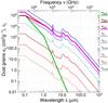 |
Fig. 1 Opacities of grains (per gram of dust) and model radial optical depths. Subscripts on the curve labels (n30 to n0.03) indicate the model mass M (in M⊙). The wavelength dependence of κsca, κabs, and κext is shown by thick solid lines (see Sect. 2.1 for details). The extinction optical depths τext of the protostellar envelopes (L⋆ = 0.3 L⊙) and starless cores are indicated respectively by the three sets of dashed blue and red lines. |
The radiative transfer models of starless cores and protostellar envelopes are presented in Sect. 2, the methods of mass derivation from fitting far-infrared and submillimeter observations are introduced in Sect. 3, the results of this work are presented in Sect. 4 and discussed in Sect. 5, the conclusions are outlined in Sect. 6, and further details are found in Appendices A–E.
2. Radiative transfer models
The models were computed with the 3D Monte Carlo radiative transfer code RADMC-3D by C. Dullemond1. Spherical model geometry was chosen to simplify the problem by reducing the number of free parameters involved in the study: asymmetries in model density distribution would introduce dependence on viewing angle (e.g., Men’shchikov & Henning 1997; Men’shchikov et al. 1999; Stamatellos et al. 2004) and hence increase the uncertainties of derived parameters. Isotropic scattering by dust grains was considered.
Grids of models for starless cores and protostellar envelopes were constructed, covering the ranges of masses M (0.03−30M⊙) and luminosities L (0.03−30 L⊙) relevant for both low- and intermediate-mass star formation. The masses and luminosities were sampled at the values of 0.0316, 0.1, 0.316, 1, 3.16, 10, 31.6 (separated by a factor of  ); for simplicity, they will be referred to as 0.03,0.1,0.3,1,3,10,30 (M⊙, L⊙). Although the luminosity of an accreting protostar depends on its mass, the goal is to separate the effects of masses and luminosities.
In addition to isolated models, their embedded variants were constructed by implanting the isolated models into the centers of larger spherical background shells of uniform densities, in order to simulate the fact that stars form within their dense parental clouds that shield the embedded objects from the interstellar radiation field. All models were put at a distance D = 140 pc of the nearest star-forming regions.
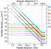 |
Fig. 2 Density structure of the model starless cores and protostellar envelopes. Subscripts on the curve labels (n30 to n0.03) indicate the model mass M (in M⊙). The dashed vertical line shows the outer boundary radius R = 104 AU for all models. Embedded models are implanted in larger uniform-density clouds with an outer boundary at 3 × 10⁴ AU. The dashed horizontal lines continue the densities of starless cores within the innermost radial zone. The dashed diagonal lines continue the densities of protostellar envelopes towards the radius of the inner dust-free cavity R0, whose size depends on the model temperature profile Td(r) (cf. Fig. 3) and adopted dust sublimation temperature (TS = 103 K). In other words, the dashed diagonal lines visualize the range of densities and radial distances over which the inner boundary R0 is located for L⋆ spanning the entire range 0.03 − 30 L⊙ (see Eq. (1)). |
2.1. Dust properties
Properties of the real astrophysical dust grains are poorly known and they are unlikely to be universal in the different star-forming regions observed. The standard mass derivation methods ignore many complications related to the cosmic dust grains, assuming just a simple power-law opacity across all bands being fitted. For example, the presence of very small, stochastically heated grains is neglected (e.g., Desert et al. 1990); the contribution of these grains to the emission of starless cores and protostellar envelopes can become significant at λ ≲ 100 μm (e.g., Bernard et al. 1992; Siebenmorgen et al. 1992). For consistency with the mass derivation methods and previous studies of star formation, this model study adopts tabulated absorption opacities κabs for grains with thin ice mantles (Ossenkopf & Henning 1994), corresponding to coagulation time t = 105 yr and number density nH = 106 cm-3 (Fig. 2).
The opacity values at long wavelengths λ> 70 μm were replaced with a power law κλ ∝ λ-2; the modification aimed at testing the widely used assumption on the power-law far-infrared opacities  . At short wavelengths (0.1<λ< 1 μm), the opacities were extrapolated with a power law κλ ∝ λ-0.87 based on the last tabulated values. Although dust scattering is unimportant in the far-infrared, scattering opacities were constructed to resemble the values and wavelength dependence κsca ∝ λ-4 of typical dust grains. The resulting dust opacity at λ> 70 μm was parameterized by κ0 = 9.31 cm2 g-1 (per gram of dust), λ0 = 300 μm, and β = 2, with the maximum opacities limited by 105 cm2 g-1 (Fig. 1).
2.2. Density distributions
The density structure of starless cores was approximated by an isothermal Bonnor-Ebert sphere (Bonnor 1956) with a temperature of 7 K and a central density of 5.2 × 10⁻¹⁸ g cm-3. This somewhat arbitrary choice of ρ(r) gives just a simple and convenient functional form (Fig. 2) resembling the observed flat-topped density profiles of starless cores (e.g., Alves et al. 2001; Evans et al. 2001). The issue of the gravitational instability (or stability) of the model cores is irrelevant for this study of the mass derivation methods. Protostellar envelopes were modeled as infalling spherical envelopes with the power-law densities ρ(r) ∝ r-2 (e.g., Larson 1969; Shu 1977) around a central source of accretion energy (Fig. 2).
Model dust densities were scaled to obtain the desired grid of masses 0.03,0.1,0.3,1,3,10, and 30 M⊙ using the standard dust-to-gas mass ratio η = 0.01. The outer boundary of all the models was placed at the same distance of R = 104 AU, beyond which their density either changed to zero (isolated models) or remained constant until RE = 3 × R (embedded models). The embedding cloud density was set equal to ρ(R) (Fig. 2), which corresponds to the denser models (i.e., more massive) being formed in a denser environment. Most of the mass of the model starless cores and protostellar envelopes (96% and 90%, respectively) is contained in their outer parts (0.1 R<r<R).
For the starless cores, the inner boundary was arbitrarily set to R0 = 50 AU, as their densities are essentially constant and hence do not need to be resolved at smaller radii. The inner boundary of the dusty protostellar envelopes is defined by the dust sublimation temperature TS ~ 103 K. An exact value of TS depends on the chemical composition and sizes of dust grains and so does the radius R0 of the inner dust-free cavity. For the purpose of this study, it is adequate to adopt a single value TS = 103 K. With the model κν and ρ(r) (Sect. 2.1), the resulting radiative-equilibrium temperatures (Fig. 3) lead to the inner boundaries of the dusty protostellar envelopes that are fairly accurately described by a simple formula, ![\begin{equation} R_{0} = 2 \left[\left(M/M_{\sun}\right) \left(L_{\star}/L_{\sun}\right)\right]^{1/3} {\rm AU}. \label{inner.boundary} \end{equation}](/articles/aa/full_html/2016/09/aa28122-16/aa28122-16-eq69.png) (1)The model space between the inner and outer boundaries was discretized by nonuniform grids with the relative zone sizes δlog r that smoothly varied from 0.6 to 0.02 (100−150 zones) for starless cores and from 0.002 to 0.06 (200−300 zones) for protostellar envelopes.
(1)The model space between the inner and outer boundaries was discretized by nonuniform grids with the relative zone sizes δlog r that smoothly varied from 0.6 to 0.02 (100−150 zones) for starless cores and from 0.002 to 0.06 (200−300 zones) for protostellar envelopes.
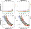 |
Fig. 3 Radiative-equilibrium dust temperature profiles of starless cores (upper) and protostellar envelopes (lower) for the isolated models (left) and their embedded variants (right). Subscripts of the curve labels (T30 to T0.03) indicate the model mass M (in M⊙). The dashed horizontal lines in the upper panels continue the profiles of starless cores within the innermost radial zone. The dashed vertical line shows the outer boundary radius R = 104 AU of all models. The maximum temperature and the inner boundary of the dusty protostellar envelopes are defined by the adopted dust sublimation temperature TS = 103 K. Three dashed horizontal lines in the lower panels indicate the range of radial distances over which the boundaries R0 of the dust-free cavities are located for the model luminosities in the entire range of 0.03 − 30 L⊙ (see Fig. 2). For protostellar envelopes with the same M, the “hotter” profiles correspond to higher L⋆, larger R0 (cf. Eq. (1)), and lower radial optical depths |
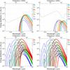 |
Fig. 4 Spectral energy distributions starless cores (upper) and protostellar envelopes (lower). Shown are the background-subtracted fluxes for the isolated models (left) and their embedded variants (right). Subscripts of the curve labels (F30 to F0.03) indicate the model mass (in M⊙). For protostellar envelopes of the same mass, the SEDs with higher fluxes correspond to higher accretion luminosities L⋆ (0.03, 0.1, 0.3, 1, 3, 10, 30 L⊙). Dashed lines indicate the fluxes of the ISRF that were integrated over the projected area of either the isolated models or the embedding clouds. |
2.3. Radiation sources and optical depths
All models were illuminated from the outside by an isotropic interstellar radiation field (Black 1994) with the “strength” parameter G0 = 1 (e.g., Parravano et al. 2003). The bolometric luminosity of the interstellar radiation field (ISRF) entering the isolated models at R amounted to LISRF = 1 L⊙, whereas that crossing the boundary of embedding clouds at RE was 9 L⊙.
In addition to the external radiation field, the models of protostellar envelopes were assumed to be heated at their centers by a blackbody source of luminosity L⋆ of 0.03,0.1,0.3,1,3,10, and 30 L⊙ with an effective temperature of T⋆ = 5770 K. Actual values of T⋆ are unimportant, as the sources of accretion energy are surrounded by the completely opaque dusty envelopes reprocessing the hot radiation to T ≲ 103 K very deep in their interiors.
Distribution of optical depths within dusty envelopes is one of the main parameters (along with the density structure) for the transfer of radiation and resulting radiative-equilibrium temperatures. All models are quite opaque at visible wavelengths, with radial optical depths τV ≈ 3−3 × 10³ for starless cores and τV ≈ 500−6 × 10⁵ for protostellar envelopes of different masses and luminosities (Fig. 1). At the far-infrared wavelength of 100 μm, starless cores with M< 3 M⊙ are transparent, whereas the ones with M ≳ 3 M⊙ are optically thick towards their centers. All protostellar envelopes are optically thick at 100 μm and some of them (with M ≳ 0.3 M⊙) are even opaque at 500 μm towards their centers. Sizes of the dust-free cavities of protostellar envelopes increase with the luminosity of their central energy sources (cf. Eq. (1), Fig. 2), thus the optical depths of the envelopes decrease, approximately as  .
.
High far-infrared optical depths of the model starless cores and protostellar envelopes are localized within relatively small spherical zones around their centers. Angular radii of the opaque dusty zones in the protostellar models can be described (at 70−500 μm) by a simple empirical expression 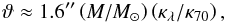 (2)which can also be used (within a factor of 1.5−2) for the high-mass models of starless cores of 3,10, and 30 M⊙, in which the opaque zone exists only at λ ≤ 70,160, and 250 μm, respectively.
The density profiles ρ(r) ∝ r-2 of the protostellar envelopes are similar to those of the starless cores for r ≳ 0.1 R (Fig. 2). Therefore, whenever an inner opaque zone exists in the objects, its mass obeys m(ϑ) ∝ ϑ, hence the fractional mass is the fractional radius and, using Eq. (2), can be written as  (3)where ϑ, D, and R are in units of arcsec, pc, and AU, respectively. At λ ≲ 100 μm, the opaque zone of high-mass objects extends over a large fraction of their mass. This means that the standard assumption of the far-infrared transparency is severely violated for massive objects. Protostellar envelopes with M< 3 M⊙ have small opaque zones that contain little mass and thus they cannot substantially affect the standard methods of mass derivation.
2.4. Temperature distributions
The models of starless cores and protostellar envelopes acquire radiative-equilibrium dust temperatures Td(r) shown in Fig. 3. In the adopted isotropic ISRF, the radiative-equilibrium temperature of dust grains with the model opacities from Fig. 1 is Td = 17.4 K, the value that the isolated models and embedding clouds acquire at their outer boundaries in the limit τλ → 0. The lower mass models of starless cores are transparent and thus almost isothermal. Their higher mass counterparts develop steeper temperature gradients under the outer boundaries of the isolated models and embedding clouds and lower temperatures in their interiors (Fig. 3).
Displaying the same behavior under their outer boundaries, protostellar envelopes of all masses develop steep temperature gradients towards the inner boundary (Fig. 3). Higher accretion luminosities make the dust hotter and thus, with the adopted dust sublimation temperature TS = 103 K, the boundary of the inner dust-free cavity shifts towards larger radial distances (cf. Eq. (1)). An analytical approximation of the profiles Td(r) for protostellar envelopes can be found in Appendix A.
Differences between the isolated and embedded models are highlighted by their different temperature distributions at the outer model boundary (Fig. 3). The temperatures of embedded models at r = R are significantly lower than those of the isolated models, owing to the absorption of ISRF in the embedding clouds (R<r ≤ RE). The denser the embedding cloud is, the lower Td(R) is and the greater the contrast to the isolated model (Fig. 3). As the bulk of the mass of the models is contained in the outer parts, the differences in the temperature profiles between the isolated and embedded models can greatly affect their observational properties, such as the images and total (integrated) fluxes.
2.5. Spectral energy distributions
After computing the self-consistent radiative-equilibrium dust temperature distributions Td(r) from the radiative transfer models, observables – such as the intensity maps ℐν and total fluxes Fν – were obtained by a ray-tracing algorithm in separate runs of RADMC-3D. Effects of the Monte Carlo noise on Fν, evaluated from the standard deviations about the azimuthally averaged intensity profiles Iν(ϑ), are below 0.003% and 3% for the starless cores and protostellar envelopes, respectively, in all models and wavebands.
To emulate the standard observational procedure of flux measurements, Fν were integrated from the background-subtracted model images ℐν. The model background  was evaluated as an average intensity
  within a δR′-wide annulus placed just outside the outer model boundary (R′>R). In practice, the annulus was one pixel in width (δR′ = 0.47″) and it was detached from the boundary by one additional pixel. For the isolated models,
  is the intensity of the isotropic ISRF, whereas for the embedded models, is determined by both
  and the transfer of radiation in the background cloud (R′ ≤ r ≤ RE) along the rays passing through the annulus. Inaccuracies inherent in the standard algorithm of background subtraction are discussed in Sect. 5.2 and Appendix B.
Spectral energy distributions (SEDs) of the models of starless cores and protostars are shown in Fig. 4. The SED shapes depend on the density and temperature distributions (Figs. 2 and 3). Large differences between the SEDs for the isolated and embedded cores are mainly caused by differences in their temperature profiles near the model boundary. The SEDs of protostellar envelopes are affected by the same effects to a much lesser degree as their density profiles are centrally peaked and their temperature profiles are dominated by the internal radiation source. The SEDs of the models of different masses and luminosities show a large variety of shapes in the far-infrared domain (Fig. 4) due to varying optical depths and temperatures.
Providing a useful reference in our analysis, additional ray-tracing runs of RADMC-3D computed the fluxes of isothermal models. These are the same models described above (Fig. 2), in which self-consistent temperature profiles (Fig. 3) have been replaced with their mass-averaged values: 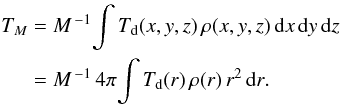 (4)The resulting total fluxes of the isothermal models are denoted Fν(TM).
3. Fitting source fluxes and intensities
In observational studies, after obtaining multiwavelength images ℐν and integrating background-subtracted (and deblended) fluxes Fν of extracted sources, their spectral distributions need to be fitted to derive fundamental physical parameters, such as the source mass and luminosity.
The standard technique uses the well-known formal solution of the radiative transfer equation that can be written as 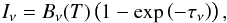 (5)where Iν is the observed specific intensity, T is the homogeneous temperature of an object, Bν(T) is the blackbody intensity, and τν is the optical depth of the object. After obtaining an image ℐν ≡ Iνij, the total flux Fν = ∫ℐν dΩ can be integrated over the solid angle Ω subtended by the object. For constant intensity, it reduces to Fν = Iν Ω. A critical assumption used in the derivation of Eq. (5) is that the object is homogeneous in temperature, whereas the temperatures of the astrophysical objects are actually nonuniform (cf. Fig. 3).
Two methods and two fitting models were explored in this work that have been used in observational studies of star formation to estimate source temperatures and masses.
3.1. Fitting total fluxes Fν
In this method, the total fluxes Fν are integrated from background-subtracted and deblended images ℐν of source intensities and then are fitted to estimate source mass as one of the fitting parameters. With the adopted parameterization of the power-law opacity κν = κ0(ν/ν0)β, it is possible to write Eq. (5) in the form  (6)where η is the dust-to-gas mass ratio and D is the source distance. The fitting model of Eq. (6) with five parameters (T, M, β, D, Ω) is referred to as modbody in this paper. After fitting Fν and estimating the model parameters, the average column density NH2 can be obtained from M = μmHNH2D2Ω, where μ = 2.8 is the mean molecular weight per H2 molecule and mH is the hydrogen mass.
With an additional assumption that measured fluxes Fν represent optically thin emission2, Eq. (6) can be written as  (7)The fitting model of Eq. (7) with four parameters (T, M, β, D) is referred to as thinbody in this paper. By the definition (τν ≪ 1), it produces only fits with the modified blackbody shapes κνBν(T) that are scaled up or down, depending on M. Obviously, the modbody fits with τν ≪ 1 produce the same shapes as the thinbody model does, whereas the modbody fits with τν ≫ 1 resemble a blackbody Bν(T). In the intermediate (semi-opaque) cases, the short-wavelength parts of the fitted curves can be described by Bν(T) while morphing into κνBν(T) at long wavelengths where the radiation becomes optically thin. With more flexible shapes, modbody can give better fits of the data, but it does not necessarily lead to good estimates of temperatures and masses.
After fitting fluxes with a modbody or thinbody model, an estimate of TF and the corresponding mass MF are obtained. For the realistic objects with strongly nonuniform temperatures Td(r) (Fig. 3), emerging fluxes Fν are heavily distorted from the simple shapes of the fitting models, hence these models are inadequate and an estimate of TF does not guarantee that MF is close to the true mass M. For the purpose of obtaining accurate MF ≈ M, it is necessary (but not sufficient) to have TF ≈ TM, i.e., it is possible to interpret T in Eq. (7) as the mass-averaged TM from Eq. (4). In fact, assuming τν ≪ 1 in the far-infrared, the observed fluxes contain emission of all dust grains, which is proportional to the mass of dust at different Td in the entire volume of an object: 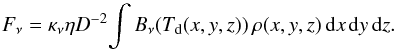 (8)Equations (7) and (8) can immediately be combined into a definition of the mass-averaged intensity BνM. Since Bν(T) ∝ T in the Rayleigh-Jeans domain, the equations are also readily converted into TM from Eq. (4). In the model objects studied here, differences between BνM and Bν(TM) quickly become negligible beyond the peak wavelength of the latter (λ≳2 λpeak). Therefore, TM is fully consistent with the fitting models at long wavelengths.
3.2. Fitting image intensities Iν
In this method, it is possible to fit pixel intensity distributions Iνij of the background-subtracted and deblended images ℐν of a source3, to derive a map of its column densities  and then the source mass
 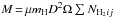 . It is convenient to express the modbody and thinbody models from Eqs. (6) and (7) as functions of the pixel column density NH2:
 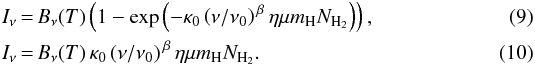 In this formulation, both models have only three fitting parameters (T, NH2, β) in contrast to the case where total fluxes are fitted (five parameters for modbody in Eq. (6) and four parameters for thinbody in Eq. (7); see Sect. 3.1). Furthermore, limited angular resolutions of real images makes the results of fitting Iν depend sensitively on the degree to which a source is resolved.
For fully resolved sources, such as the model objects used in this work, relatively small pixels sample completely independent intensities from different rays. For progressively lower angular resolutions, intensities within a beam become increasingly blended together. Radiation with different temperatures gets mixed not only along the line of sight, but also in the transverse directions, in the plane of the sky. For unresolved objects with intrinsic temperature gradients, radiation from the entire object becomes heavily blended, leading to strong distortions of their spectral intensity distributions.
An important assumption used in the derivation of NH2ij is a constant temperature Td(x,y,z) along the lines of sight within a certain radial distance from a pixel (i,j). The distance depends on the angular resolution of images: for less resolved sources, temperatures from a larger environment of the pixel contribute to its intensity. With low optical depths τν ≪ 1 in the far-infrared, emission is observed from the entire column of dust grains at (i,j) with different temperatures Td(z) along the line of sight. The reasoning associated with Eq. (8) can be applied to show that T in Eq. (10) is consistent with the column-averaged temperature 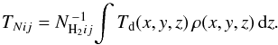 (11)A mass-averaged temperature, equivalent to that from Eq. (4), can be obtained as
 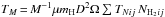 .
.
3.3. Variable and fixed parameters
In most studies, the opacity slope β has been kept fixed in the fitting process to reduce the number of free parameters and improve the robustness of derived parameters. Following this practice, Sect. 4 presents and discusses only the results of fitting with a fixed opacity slope. When fitting intensities Iν with β fixed, the number of free variable parameters becomes γ = 2 for both thinbody and modbody models (T, NH2). When fitting fluxes Fν, distance D is also assigned a fixed value to further reduce the degrees of freedom, although astronomical distances are poorly known. The number of free variable parameters is thus γ = 2 for thinbody (T, M) and γ = 3 for modbody (T, M, Ω).
In practice, after measuring Fν = ∫Iν dΩ, the solid angle Ω over which Iν were integrated is known4 and its value can be fixed, reducing γ for modbody to two free variables (T, M). In this model study, one could also keep Ω = π (R/D)2 constant, as the true values of R and D are known; however, modbody would then become completely equivalent to thinbody. Indeed, fixing Ω of transparent objects at accurate (or even overestimated) values means that the optical depths in Eq. (6) are very small (τν = κνηMD-2Ω-1 ≪ 1), which effectively converts modbody into thinbody. Only when fixing strongly underestimated values Ω ≪ π (R/D)2, the far-infrared τν become large enough to produce any noticeable differences between modbody and thinbody. This work investigates qualities of two different models, hence Ω was allowed to vary in all modbody fits of Fν.
When fitting pixel intensities Iν instead of Fν, the far-infrared τνij within most of the image pixels (i,j) are small, even for perfectly resolved sources. For poorly resolved or unresolved sources, radiation within the beams gets diluted and maximum values of τνij in the images become smaller. All models of starless cores and protostellar envelopes contain 96% and 90% of their masses, respectively, in their outer parts (r ≳ 0.1 R, Fig. 2). Intensities in the outer parts of the source images come mostly from the pixel columns of dust with τνij ≪ 1 in the far-infrared. Only in the models with M ≳ 3 M⊙ do they become substantially affected by the radiation from the central opaque zone (Sect. 2.3). As a result, the masses derived from fitting Iν are almost the same (within ~20%) for both fitting models and hence only the thinbody results are presented for this method.
3.4. Data points and their subsets
Fitting was executed for a set of the total model fluxes {Fλi} or pixel intensities {Iλi}(i = 1,2,...,6) at the Herschel wavelengths λi of 70, 100, 160, 250, 350, and 500 μm. In this model-based study, the intensities and fluxes of numerical models have essentially no measurement errors. It makes sense, however, to make their uncertainties resemble typical observational values, hence to get an idea of realistic inaccuracies of the estimated parameters (masses, temperatures). Before the fitting, the model intensities and fluxes were assigned an additional (optimistic) uncertainty of 15%, a value similar to the levels of calibration errors in real observations (e.g., with Herschel). The above uncertainties were associated with the exact data points to see how typical data uncertainties translate into the resulting error bars of the derived parameters. Extra uncertainties come from the fact that the dust-to-gas ratio η, reference opacity κ0, and distance D, which are used in the fitting models (Sects. 3.1, 3.2) but held constant, are actually poorly known. Conservatively assuming that the quantities have random and independent uncertainties of 20%, the latter were added in quadrature to those of the derived masses, for the same purpose of obtaining the total resulting mass uncertainties.
To isolate the effects of temperature gradients in starless cores and protostellar envelopes (Fig. 3), the fitting was done for several subsets of data, removing some (or none) of the shortest-wavelength points from the fitting process. The data subsets are denoted Φn = {Yλi}, where Yλi is either Fλi or Iλi and n is the number of the longest wavelengths used in the fitting5. Fits of total fluxes were considered successful (acceptable) and their results are shown below, if χ2 ≤ n−γ + 1, with the last term added to allow testing χ2 for zero degrees of freedom (n = γ). Fits of image intensities were considered successful, if the same goodness condition was fulfilled in all pixels within an object. These results, as well as the somewhat less reliable results with n−γ + 1 <χ2< 10 in some pixels are presented below. Details of the fitting algorithm can be found in Appendix C.
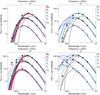 |
Fig. 5 Fluxes of the isolated starless cores (upper) and protostellar envelopes (lower) fitted with the thinbody (left) and modbody (right) models. The fluxes for the 0.03, 0.3, and 3 M⊙ cores and envelopes (with L⋆ = 1 L⊙) from Fig. 4 are shown as black triangles, squares, and circles, respectively. Successful fits (Sect. 3.4) using different subsets Φn of fluxes are indicated by the solid and dashed lines of different widths and colors. The thin black curves show the flux distributions for the isothermal models where the actual model temperatures (Fig. 3) were replaced with their mass-averaged values: Td(r) = TM (16.3,13.2,9.2 K for starless cores and 18.1,15.6,12.3 K for protostellar envelopes). |
4. Results
This section describes derived parameters for both starless cores and protostellar envelopes, obtained from acceptable fits for all subsets Φn (Sect. 3.4) for both modbody and thinbody (Sect. 3.1). Results for the isothermal models are presented in Appendix D. To evaluate the effects of the uncertain far-infrared opacity slope, results are shown for β = 2 used in the radiative transfer modeling and for two other β values (1.67, 2.4), differing from the true value by a factor of 1.2. Results obtained with variable fitting parameter β are described in Appendix E.
Masses derived from fitting images ℐν of objects with temperature gradients must depend on their angular resolutions (Sect. 3.2). To investigate this effect, the model images with pixels of 0.47″ were convolved with Gaussian beams of 1, 36, and 144″ (FWHM) and then resampled to 1, 12, and 48″ pixels, respectively. For the objects with diameters of 142″ (2 × 10⁴ AU, Fig. 2), the three variants represent resolved, partially resolved, and unresolved cases.
In this paper, the term uncertainties refers to the error bars of measured or derived quantities, the term inaccuracies (sometimes simply errors) refers to the deviations of the derived quantities from their model values, and the term biases denotes variable systematic dependences of inaccuracies across the ranges of model parameters (M, L, TM).
4.1. Selected examples
Examples of the fits of Fν for the isolated starless cores and protostellar envelopes with masses of 0.03, 0.3, and 3 M⊙ are shown in Fig. 5. Although the qualitatively similar plots for embedded models are not presented, their derived parameters and uncertainties are described in Sect. 4.2.
Flux distributions of the isolated starless cores (Fig. 4) are similar to those of the modified blackbodies κνBν(TM). The fits for a low-mass core with M = 0.03 M⊙ shown in Fig. 5 are identical for all subsets Φn since the core is nearly isothermal, with Td(r) very similar to its TM = 16.3 K. Fluxes of the higher-mass cores of 0.3 and 3 M⊙ display larger deviations from the fluxes Fν(TM) of isothermal models for larger subsets Φn (n = 3 → 6). The shapes of Fν become “hotter” because of the steeper temperature profiles (Sect. 2.4) at the outer boundary (Fig. 3). For a massive core of 3 M⊙, discrepancies between Fν and Fν(TM) at λ ≲ 160 μm reach factors ≳ 5.
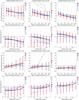 |
Fig. 6 Temperatures TF and masses MF derived from fitting Fν of both isolated and embedded starless cores vs. the true model values of TM and M for three β values (1.67, 2, 2.4). For various subsets Φn of fluxes, results from successful thinbody and modbody fits (Sect. 3.4) are displayed by the colored and gray lines, respectively. Error bars represent the 1 × σ uncertainties of the derived parameters returned by the fitting routine combined with the assumed ± 20% uncertainties of η, κ0, and D (Sect. 3.4). The black solid lines show the locations where TF and MF are equal to the true values. To preserve clarity of the plots, much less accurate modbody results are displayed only for correct β = 2 and without error bars. |
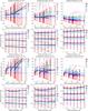 |
Fig. 7 Temperatures TF and masses MF derived from fitting Fν of both isolated and embedded protostellar envelopes (with the true masses M of 0.03, 0.3, and 3M⊙) vs. the true model values of TM and L for three β values (1.67, 2, 2.4). Results from successful thinbody and modbody fits for various subsets Φn of fluxes (Sect. 3.4) are displayed by the colored and gray lines, respectively. See Fig. 6 for more details. |
Flux distributions of an isolated protostellar envelope with M = 0.03 M⊙ (Fig. 4) display various shapes that are quite different from those of κνBν(TM), whereas for a more opaque envelope of 3 M⊙ they become similar to the modified blackbody shapes. The protostellar fits (Fig. 5) show greater deviations for larger subsets Φn (n = 3 → 6), much larger than those of starless cores. Differences between Fν and Fν(TM) reach orders of magnitude at λ ≲ 100 μm. The shapes appear much “hotter” owing to Td ~ 100−103 K (Sect. 2.4) deep inside the envelopes (Fig. 3). The lower-mass protostellar envelopes are more transparent and the hot emission greatly distorts Fν at λ ≲ 250 μm.
4.2. Properties derived from fitting fluxes Fν
Isolated starless cores, β = 2 (Fig. 6). For the low-mass, transparent cores (M → 0.03 M⊙), quite accurate values TF ≈ TM and MF ≈ M are derived for all subsets Φn. For the denser, more opaque cores (M → 30 M⊙), derived TF and MF become more over- and underestimated, respectively, as the spectral shapes of Fν become much wider and distorted towards shorter wavelengths (Fig. 4). The biases and inaccuracy of the estimates depend on the subset Φn, with the least inaccurate TF and MF obtained for the thinbody fits of Φ2. However, the biases of the parameters across the entire mass range remains fairly strong. Derived masses of the starless cores are underestimated within a factor of 2 for 1 <M ≤ 3 M⊙ and factor of 5 for 3 <M ≤ 30 M⊙.
Embedded starless cores, β = 2 (Fig. 6). For the low-mass, transparent cores (M → 0.03 M⊙), MF are underestimated by a factor of 1.35 for all subsets Φn, although TF are quite accurate because the standard observational procedure of background subtraction ignores the fact that embedding backgrounds tend to be rim-brightened at their outer boundary R (Appendix B, Sect. 5.2). The embedded cores have Td(r) that are quite flat across their boundary for all masses (Fig. 3). Having no flux distortions caused by nonuniform temperatures (Fig. 4), the Fν peaks of the most massive cores (M → 30 M⊙) move towards the longest wavelength (λ6 = 500 μm), which leads to TF and MF that are under- and overestimated, respectively.
Isolated protostellar envelopes, β = 2 (Fig. 7). Emission of the hot dust with Td ~ 100−103 K greatly skews their Fν towards shorter wavelengths (Fig. 4). This becomes especially significant for the lower mass, more transparent envelopes (M → 0.03 M⊙, L⋆ → 30 L⊙) that produce hotter dust over a much larger volume (Fig. 3). The thinbody fits of larger subsets Φn (n = 3 → 6), lead to errors in TF and MF that reach factors of 1.6 and 3, respectively. The smallest subset Φ2 is unaffected by the hot emission and it produces fairly accurate thinbody estimates of TF and MF (for all M and L⋆) within factors of 1.1 and 1.3, respectively.
Embedded protostellar envelopes, β = 2 (Fig. 7). Results are qualitatively similar to those of the isolated envelopes, although with larger inaccuracies. Derived MF are underestimated by at least a factor of 1.5, mostly due to over-subtraction of the rim-brightened embedding background (Appendix B, Sect. 5.2). Although the envelopes have Td(r) that are quite flat across their boundaries (Fig. 3), their derived parameters are greatly affected by the skewed Fν owing to the hot dust deep in their interiors. The thinbody fits of large subsets Φn (n = 3 → 6) lead to inaccuracies in TF and MF as large as factors of 1.4−1.8 and 3−5, respectively. The most accurate TF and MF, obtained for the smallest subset Φ2, are underestimated within factors of 1.2 and 2.
Effects of the adopted opacity slope β on the estimated parameters are similar for both starless cores (Fig. 6) and protostellar envelopes (Fig. 7). Although detailed behavior of the differences with respect to the above results for true β = 2 depends on the subset Φn, clear general trends can be seen. Shallower slopes (β = 1.67) lead to an increase in TF and thus MF becomes smaller, whereas steeper slopes (β = 2.4) lead to a decrease in TF and hence MF becomes larger, in both cases by a factor of approximately 2.
The thinbody fitting model produces much better overall results than modbody does. Parameters estimated with modbody become so incorrect that they may be considered completely unusable. The importance of estimating accurate mass-averaged temperatures TM for deriving correct masses MF is illustrated by the isothermal models presented in Appendix D.
4.3. Properties derived from fitting images ℐν
This section presents results for both starless cores and protostellar envelopes, obtained from successful fits of the background-subtracted ℐν for all subsets Φn, for only the thinbody fitting model. Derived modbody masses are practically the same as the thinbody masses, because the bulk of the model mass is in optically thin regions (Sect. 3.3). Effects of the adopted far-infrared opacity slopes are the same as when fitting Fν (Sect. 4.2): under- or overestimating β by a factor of 1.2 gives masses Mℐ that are systematically under- or overestimated by a factor of 2. The method of fitting images ℐν, thereby deriving  , and afterwards integrating source mass Mℐ brings clear benefits for well-resolved starless cores with nonuniform temperatures, compared to the other method (Sect. 4.2) of first integrating total fluxes Fν from ℐν (losing all spatial information) and then estimating MF from the fitting model.
Isolated starless cores, β = 2 (Fig. 8). For the fully resolved models, derived Tℐ and Mℐ have fairly good accuracy and little bias for acceptable fits, although the range of the latter for larger Φn (n = 3 → 6) shrinks to the lowest masses. As the transparent low-mass cores (M → 0.03 M⊙) are almost isothermal, derived Tℐ and Mℐ perfectly agree with TM and M for any subset Φn. Massive cores with more variable Td(r) (Fig. 3) also have significant variations of Td(z) along the line of sight at pixel (i,j). Emission of hot dust skews the spectral shapes of Iνij towards shorter wavelengths, even more so at the high-mass end. The most accurate masses are obtained for Φ2, whereas larger Φn (n = 3 → 6) give increasingly incorrect Tℐ and Mℐ. With degrading angular resolutions, the inaccuracies and biases increase, especially for M → 30 M⊙ and larger Φn (n = 3 → 6). As expected, in the limiting case of unresolved objects the results approach those obtained with the method of fitting fluxes Fν (Fig. 6).
Embedded starless cores, β = 2 (Fig. 8). For the fully resolved models, derived Tℐ have fairly good accuracy and little bias for the acceptable fits, although the range of the latter for larger Φn (n = 3 → 6) shrinks to even lower masses than for the isolated models. Showing no particularly large bias over almost the entire range of model masses, Mℐ are underestimated by a factor of 1.3 owing to the standard observational procedure of background subtraction (Appendix B, Sect. 5.2). Derived parameters of the models do not depend on angular resolutions, as they have relatively flat Td(r) across their boundaries (Fig. 3), hence the spectral distortions of Iνij are negligible.
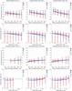 |
Fig. 8 Temperatures Tℐ and masses Mℐ derived from fitting images ℐν of both isolated and embedded starless cores vs. the true model values of TM and M for correct β = 2. The three columns of panels present results for three angular resolutions (resolved, partially resolved, and unresolved cases) and for various subsets Φn of pixel intensities. Error bars represent the 1 × σ uncertainties of the derived Tℐ and Mℐ (computed over all pixels as the NH2-averaged errors of TNij and integrated errors of NH2, correspondingly), combined with the assumed ± 20% uncertainties of η, κ0, and D (Sect. 3.4). Less reliable results (n−γ + 1 <χ2< 10 in some pixels) are shown without error bars. See Fig. 6 for more details. |
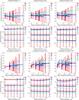 |
Fig. 9 Temperatures Tℐ and masses Mℐ derived from fitting images ℐν of both isolated and embedded protostellar envelopes (with the true masses M of 0.03,0.3, and 3 M⊙) vs. the true model values of TM and L for correct β = 2. The three columns of panels present results for three angular resolutions indicated (resolved, partially resolved, and unresolved cases). See Fig. 8 for more details. |
Isolated protostellar envelopes, β = 2 (Fig. 9). For the fully resolved models, derived Tℐ and Mℐ are very accurate across all masses and luminosities. With degrading angular resolutions and for larger Φn (n = 3 → 6) the inaccuracies and biases increase quite considerably. The accretion energy released in the envelopes centers heats the dust to TS ~ 103 K, making Td(r) strongly nonuniform. For the lines of sight passing through the inner radial zones, the hot emission skews the Iνij shapes towards shorter wavelengths. For the unresolved envelopes, the results become similar to those obtained with the method of fitting fluxes Fν (Fig. 7).
Embedded protostellar envelopes, β = 2 (Fig. 9). For the fully-resolved models, derived Tℐ are slightly less accurate for the acceptable fits than in the case of the isolated envelopes. The range of the latter in more massive models for larger Φn (n = 3 → 6) shrinks towards higher L⋆. The most accurate Mℐ, obtained for Φ2, are underestimated by a factor of 1.45, mostly because of the over-subtraction of the rim-brightened background (Appendix B, Sect. 5.2). For the partially resolved and unresolved envelopes, the most accurate Mℐ (for Φ2) are underestimated by factors of 1.5−2, whereas fitting larger Φn (n = 3 → 6) leads to errors by factors of 4−5.
5. Discussion
Spectral flux and intensity distributions of the radiative transfer models of the starless cores and protostellar envelopes (0.03−30 M⊙,L⊙) were fitted using the modbody and thinbody models. Derived values of the fitting parameters were then compared to their true values to quantify the qualities of the mass derivation methods, fitting models, and various sources of errors.
As shown in Sect. 4, large intrinsic inaccuracies and biases need to be taken into account when applying the methods of mass derivation to the observed sources. In addition to being affected by nonuniform temperatures, estimated masses are also affected by the adopted value of β and subset of data points Φn, as well as by the removal algorithm of the background emission of an embedding cloud. In the method of fitting fluxes Fν, the masses depend on the fitting model, whereas in the method of fitting images ℐν, they depend on the angular resolution.
The results of this purely model-based work discussed below may be directly applicable only to sources with very accurate measurements (with negligible errors). Real observations deal with images of relatively faint, crowded sources on strong and variable backgrounds, obtained with quite different angular resolutions, and thus they carry much larger measurement errors. Observations are substantially affected by various statistical and systematic errors, depending on the adopted source extraction method (e.g., Men’shchikov et al. 2012; Men’shchikov 2013) and especially the treatment of background subtraction and deblending. Implications for the real-life studies are considered below, whenever possible.
5.1. Mass derivation methods
In the first method, source fluxes Fν are integrated from the images ℐν, their spectral distribution is fitted, and source mass MF is estimated from the fitting model. In the second method, the pixel spectral shapes Iν of the images ℐν are fitted and the source mass Mℐ is integrated from the resulting image of column densities. For unresolved sources and the thinbody fitting model, the methods give very similar levels of inaccuracy, whereas for resolved images, the methods differ quite substantially.
When fitting Fν, the observed source emission from its entire volume is blended in the spatially integrated fluxes that retain no spatial information. For the models with strongly nonuniform Td(r) (Fig. 3), resulting heavy distortions of the spectral shapes of Fν (Fig. 4) from those of the fitting models lead to large systematic errors in estimated parameters (Figs. 6 and 7).
When fitting ℐν, it is very beneficial to have a higher angular resolution. For fully resolved objects, pixels (i,j) sample independent Iνij from different columns of dust. For the transparent lower mass models (M ≲ 0.3 M⊙), derived Mℐ are quite accurate (Figs. 8, 9). For lower resolutions, the intensity of each pixel (i,j) blends with that of its larger surroundings within the beam, not only along the line of sight. The contamination of Iνij by the more distant areas, leads to a substantial degradation of Tℐ and Mℐ, especially when fitting large Φn (n = 3 → 6). Thus, the benefits of this method are vanishing with decreasing angular resolutions.
Multiwavelength Herschel images have been used to reconstruct radial temperature and density profiles of well-resolved sources (Roy et al. 2014). Whenever such reconstructed densities are accurate enough, they can be used to obtain masses of the nearby sources. Results of this study demonstrate, however, that the simple method of fitting images ℐν is able to deliver accurate masses for spatially resolved sources (Sect. 4.3).
5.2. Background subtraction
Stars form in the densest parts of interstellar clouds, hence the embedded models of starless cores and protostellar envelopes must be more realistic than the isolated models. Although the spherical uniform-density embedding clouds are idealized, in a first approximation they account for the absorption and re-emission of ISRF, leading to realistic temperature profiles within the model objects. However, the presence of surrounding material makes it necessary to subtract its contribution to study the properties of the starless cores and protostellar envelopes alone. In observational practice, backgrounds are estimated by an average intensity in a narrow annulus placed just outside a source (cf. Sect. 2.5). Subtraction of such a flat background is not quite accurate as a transparent embedding cloud around any object always tends to be rim-brightened and resembles a crater, in contrast to a distant, physically unrelated back- or foreground. This effect is discussed in detail in Appendix B.
The actual observable depths of the background craters may be shallower, when the local (filamentary) background itself is embedded in a less dense but more extended cloud or is seen in projection onto a distant, physically unrelated back- or foreground. The rim-brightening effect gets diluted, if the column densities of the source-embedding background and of the other unrelated clouds are similar. Poorer angular resolutions also tend to smear out the effect for less resolved sources. Realistic temperature gradients within the embedding backgrounds (Fig. 3) can either reduce or increase the crater depths by ~ 10% for starless cores and protostellar envelopes, respectively (Appendix B).
For unresolved sources, the observational algorithm of background subtraction is likely to overestimate fluxes as stars are born within the gravitationally unstable densest peaks of the parent clouds. Large beams blend the object’s emission with that of its mountain-like environment, spreading the mix downhill, towards the valleys of lower cloud densities. The real background under an unresolved source must be hill-like, whereas the background values from an annulus tend to come from more distant valleys. The problem is aggravated in crowded regions, where no local source-free annuli around overlapping sources can be found and where one needs to deblend sources. Angular resolution degrades with wavelengths, hence the degree of flux overestimation becomes strongly biased towards longer wavelengths.
5.3. Nonuniform temperatures
Both fitting models make a sensitive assumption that the objects have a uniform temperature T, which seems to make them inadequate for the applications to starless cores and protostellar envelopes with nonuniform Td(r). For the purpose of the derivation of accurate masses, however, the uniform T can be interpreted as an appropriate average quantity. In the methods of fitting Fν and ℐν, the temperature is consistent with TM and TNij from Eqs. (4) and (11), respectively (cf. Sects. 3.1 and 3.2). In other words, to estimate masses MF or Mℐ that are accurate (≈M), it is necessary that the fitting returns TF or Tℐij as close as possible to the average values TM or TNij, respectively. This is clearly demonstrated in Appendix D by the accurate masses obtained for the isothermal models with Td(r) = TM.
The inhomogeneous temperatures tend to distort the spectral shapes of Fν and Iνij of the objects towards shorter wavelengths (Figs. 4 and 5). With a strong dependence of the dust emission peak on temperature (κνPBνP(T) ∝ T5), the radial zones with higher Td(r) make a much greater contribution to the observed spectral shapes. Therefore, the shapes are skewed mainly owing to the emission of those parts of the objects that have Td(r) >TM or Td(r) >TNij. In other words, distortions of the spectral shapes are caused by the dust with excess temperatures above the average values.
This is further demonstrated by additional ray-tracing observations of the models, in which the excess temperatures were removed: Td(r) → min{Td(r),TM}. Derived masses of these mostly isothermal models (not shown) are almost as accurate as those of the fully isothermal models (Appendix D), only within a few percent lower. As is expected, there is almost no dependence on the subsets Φn (n = 2 → 6), which indicates that the spectral shapes are indeed not distorted.
5.4. Fitting models
When fitting images ℐν, both fitting models are equivalent and estimated parameters are indistinguishable (Sect. 3.3). When fitting fluxes Fν, the results of this work show that thinbody generally returns far more accurate masses than modbody does for both isolated and embedded variants of starless cores and protostellar envelopes (Figs. 6 and 7).
Although the modbody fits often look better (i.e., they have smaller χ2 values), they generally bring parameters that are much more inaccurate. Indeed, the spectral shapes of Fν are skewed towards short wavelengths by emission from their hotter parts. With more free parameters, modbody describes more flexible shapes, between Bν(T) and κνBν(T). It is able to produce better fits of the distorted spectral shapes of objects with nonuniform Td(r) and hence it always tends to produce significantly over- and underestimated TF and MF, respectively (Sect. 4.2). Furthermore, most of the modbody fits have τν ~ 1 even in the far-infrared, which is fundamentally inconsistent with the radiative transfer models whose fluxes Fν represent optically thin emission (τν ≪ 1).
The thinbody model produces the best overall results and smallest biases and inaccuracies in derived TF and MF for the isolated and embedded starless cores and protostellar envelopes (Figs. 6−9). The thinbody fits are, by definition, optically thin in the far-infrared and thus consistent with the radiative transfer models. Only two variable fitting parameters of thinbody contribute to better robustness of TF and MF, compared to modbody with one extra free parameter.
Contrary to what is usually assumed in observational studies, the results show that it must be counterproductive to aim at precise fitting of the peaks and shorter wavelength parts of Iν and Fν. When the distorted shapes are reproduced more accurately, the estimates of the temperatures and masses are less accurate.
5.5. Opacity slopes
The standard methods of mass derivation ignore the presence of very small stochastically heated dust particles, assuming just a simple power-law opacity across all bands, and so do the radiative transfer models in this study. Emission of such very small grains within the real objects could enhance fluxes at 70 and 100 μm and, in effect, skew their spectral shapes farther towards short wavelengths, leading to more heavily overestimated temperatures and underestimated masses.
Various compositional and structural properties of real cosmic dust grains in different environments may lead to far-infrared opacity slopes that are different from β ≈ 2 (expected for small compact spherical grains) and even to wavelength-dependent βλ. This study explored three constant values (1.67, 2.0, 2.4) to probe their influence on the accuracy of derived masses. Fixing β in the fitting process reduces the number of free parameters and improves the consistency (reduces biases) of derived parameters for objects with different physical properties (M, L⋆).
With the correct β value, masses derived with the thinbody fits are generally off the true mass M, the magnitude of discrepancy depending on how much and in what direction derived temperature deviates from TM. When β is over- or underestimated by a factor of 1.2, derived masses become over- or underestimated within a factor of 2 with respect to the masses obtained using the true value β = 2. This is a direct consequence of the temperatures being under- or overestimated, correspondingly, a behavior that is easy to understand. In contrast to the thinbody fits, no clear trends with respect to the inaccuracies in the adopted β value can be found for modbody, except that it generally returns greatly over- and underestimated TF and MF.
To quantify the effects of freedom in this fitting parameter, additional fits with variable β were performed (Appendix E). As is expected, they showed much greater biases and inaccuracies in derived parameters (Figs. E.1 and E.3), as the extra degree of freedom also makes the resulting β values incorrect (Fig. E.2), the magnitude of error depending on the true values of M and L⋆. It is possible to compare these results with those obtained in previous studies focused on the relationships between the derived βF and TF (Shetty et al. 2009a,b; Juvela & Ysard 2012, and references therein). The present models of starless cores and protostellar envelopes show that the correlations of the two quantities may be both positive and negative (Fig. E.4), with almost no correlation in the case of isothermal models. They must be induced by deviations of the spectral shapes of Fν (Fig. 4) from Fν(TM) (Fig. D.1), caused by the nonuniform Td(r) (Fig. 3). For the protostellar envelopes, the correlations are non-monotonic and they may either be strongly negative or positive, depending on the luminosity.
5.6. Data subsets
For nonuniform profiles Td(r) of starless cores and protostellar envelopes (Fig. 3), better parameters are estimated with thinbody when using smaller subsets of data (n = 6 → 2) as the latter are less affected by the skewed spectral shapes. The most accurate masses are obtained by fitting just two of the longest wavelength data points; in most cases, however, a subset Φ3 produces very similar results. Larger subsets Φn (n = 2 → 6) may give slightly better MF only when fixing an incorrect β value for the lower-mass starless cores (M ≲ 1 M⊙, Fig. 6). Using the inadequate fitting model with an incorrect β, larger Φn can constrain TF to better resemble TM. For overestimated β, derived MF always shift to higher values (Fig. 7), which offsets the general opposite trend to underestimate MF and thus may give more accurate results.
Inaccuracies of the data points in real observations are usually more substantial than those assumed in this work, aggravated by the systematic uncertainties that may lead to both over- and underestimated Fν (Sect. 5.2). Background-subtracted and deblended Iν at each wavelength with different angular resolutions have independent and different systematic errors. The latter must be large and uncertain on the bright and structured backgrounds in star-forming regions. Moreover, unresolved sources are likely to include emission from clusters of objects.
Results of this model study are directly relevant to real observations only in the simplest case (which is rare) of accurate measurements with negligible errors. A blind application of the findings to real complex images may lead to incorrect results if the above caution is ignored and small subsets Φ2 of data points with large and independent measurement errors are fitted. For such data, it would be safer and more appropriate to fit a larger subset of the longest wavelength data (Φ3 or Φ4, depending on the quality of measurements). Distortions of the observed spectral shapes towards shorter wavelengths is an intrinsic property of both starless cores and protostellar envelopes, affecting all sources in star-forming regions, independently of the level of measurement errors.
It beyond the scope of this model-based work to give general recipes to observers on how to select data points to fit. This study highlights the intrinsic behavior of the mass derivation methods by eliminating the “observational layer” (with all its complications and uncertainties) between the objects and the observer. It is important to realize that the peak and shorter wavelength shapes of Iν and Fν are most skewed by the temperature excesses within objects (Sect. 5.3) and their influence has to be minimized to obtain accurate results. In view of the strong dependence of the results on Φn, it is advisable to examine fits of all subsets of data points for each observed source to estimate the robustness of the results and to possibly choose the fits giving the best mass estimate.
5.7. Mass uncertainties
To make a bridge between this purely model-based study with no measurement errors and actual observational studies and see how typical statistical errors in the input data would translate into those of the derived masses, this work assigned (fairly optimistically) ±15% errors to the model intensities and fluxes, and adopted ±20% errors in η, κ0, and D.
The uncertainties in derived masses returned by the fitting algorithm are 40−70%, depending on the subset Φn of fluxes (Figs. 6−9, D.2, D.3). For the acceptable fits of larger subsets (n = 2 → 6), the derived mass uncertainty is dominated by the 20% errors of the parameters η, κ0, and D, because the effect of the 15% measurement errors becomes smaller for the fits constrained by a larger number of independent data points. For smaller subsets (n = 6 → 2), the fits are less constrained, hence the contribution of the 15% error bars to the derived mass uncertainty becomes larger. Different subsets Φn give very similar results only for fully resolved sources with the method of fitting images ℐν (Figs. 8 and 9).
In real observations, statistical measurement uncertainties in Iν and Fν are larger than the ±15% errors assumed in this study. Furthermore, it would be more realistic to adopt uncertainties of η, κ0, and D of at least ±50%, which would raise the derived mass uncertainties well beyond 100%. By including the mass inaccuracies (of a factor of 2) induced by a 20% uncertainty in β and systematic errors (of factors of at least 2) caused by the nonuniform temperatures within the observed sources, it is clear that the absolute values of masses derived from fitting are inaccurate and uncertain (within a factor of at least 2−3). It is possible to neglect the uncertainties in η, κ0, and D, if the focus is on studying relative properties of a population of objects all at roughly the same distance within a certain star-forming cloud with homogeneous dust properties. Apart from this, however, one has to derive accurate absolute values of the most fundamental parameters to make correct and physically meaningful conclusions.
It is quite important to carefully estimate mass uncertainties: without realistic error bars, derived masses are meaningless and correct conclusions are unlikely. To go one step further and obtain an idea of the actual errors of derived masses, it is possible to construct radiative transfer models of the observed population of sources, distribute the model sources over the observed images and extract them, and finally derive their masses. Comparing derived masses with the fully known model properties, reasonable estimates of the actual errors in derived masses are obtained.
6. Conclusions
This paper presented a model-based study of the uncertainties and biases of the standard methods of mass derivation (fitting fluxes Fν and images ℐν), widely applied in observational studies of the low- and intermediate star formation. To focus on the intrinsic effects related to the physical objects, all observational complications leading to additional flux or intensity errors (filamentary and fluctuating backgrounds, instrumental noise, calibration errors, different resolutions, blending with nearby sources, etc.) were assumed to be nonexistent. As a consequence, results of this work are directly relevant only for the simplest case of bright isolated sources on faint backgrounds with negligible measurement errors. The real mass uncertainties for starless cores and protostellar envelopes are likely to be larger than those found in this work.
Embedding backgrounds of physical objects tend to be rim-brightened (i.e., resembling craters), their depths depend on the sizes of the object and embedding cloud. The standard observational procedure of flat background subtraction may give systematically underestimated Iν and Fν, and hence masses for resolved sources. Poorer angular resolutions at longer wavelengths tend to systematically overestimate Iν and Fν, and hence masses for unresolved objects, as their emission gets blended with that of the mountain-like background and possibly with other objects within the same beam.
Temperature excesses above average values TM and TNij are the primary reason for the skewness of the spectral shapes of Fν and Iνij towards shorter wavelengths. Depending on M, L⋆, β, Φn, fitting model, and angular resolution, they lead to overestimated temperatures and various biases. With the method of fitting Fν, masses become underestimated by factors 2−5. When fitting ℐν, similarly large inaccuracies are found only for unresolved objects, whereas with better angular resolutions they decrease and become very small for well-resolved objects.
When fitting ℐν, both fitting models are equivalent and estimated Mℐ are indistinguishable. When fitting Fν, thinbody gives far more accurate MF than modbody does. The latter causes such great biases and inaccuracies in TF and MF that modbody must be considered unusable.
Fixing opacity slope β reduces biases in derived parameters. When β is too high or low by a factor of 1.2, derived masses become over- or underestimated by a factor of 2 with respect to those obtained using the true β = 2. Qualitatively, this behavior is caused by the natural tendency of steeper β to produce lower temperatures, hence higher masses. Quantitatively, the factors are approximate and they may depend on some of the assumptions used in this study. Mass derivation with a free variable β should be avoided, as it tends to lead to very strong biases and erroneous masses.
Subsets Φn of data points strongly affect derived masses, except when fitting images ℐν of fully resolved sources. Given the nonuniform Td(r) of the model objects, the most accurate masses are estimated with thinbody using subsets that are as small as possible (n = 6 → 2). In real observations with substantial independent errors in different wavebands, it should be much safer and more accurate to fit slightly larger subsets (Φ3 or even Φ4). Those data points that are on the peak of their spectral distribution or on the short-wavelength side should be ignored, whenever possible, to improve the accuracy of derived masses. In practice, it is advisable to investigate fits of all subsets of data for each observed source, to verify robustness of the results and to possibly choose the best mass estimate.
Inaccuracies of the derived masses depend on the mass range considered. Dividing the range of 0.03−30 M⊙ at 1 M⊙ into the low- and high-mass objects and considering unresolved or poorly resolved sources with β = 2, the following conclusions drawn. Masses of the isolated low- and high-mass starless cores are underestimated by factors 1−1.3 and 1.3−4, respectively. The mass inaccuracies increase towards the high-mass end and for larger subsets Φn (n = 2 → 6). Masses of the embedded low-mass cores are underestimated by a factor of 1.4. They are more biased towards the high-mass end, changing from under- to overestimated within a similar factor. Masses of the protostellar envelopes are considerably biased over the range of 0.03−30 L⊙ and their inaccuracies strongly increase for larger subsets of Φn (n = 2 → 6). Masses of the isolated and embedded envelopes become underestimated by factors 2−3 and 3−5, respectively. Masses of the low-mass starless cores are likely to be determined much more accurately than those of protostellar envelopes.
Typical mass uncertainties returned by the fitting algorithm are 40−70%, adopting statistical errors of 15% for model intensities (fluxes) and optimistically assuming that η, κ0, and D were known to within 20%. If more realistic statistical errors in the measurements and parameters of at least 50% are adopted, the mass uncertainties increase well beyond 100%. Larger subsets Φn (n = 2 → 6) of independent data points are beneficial in somewhat reducing the resulting mass uncertainties. On the other hand, the larger subsets are also highly undesirable, because they escalate the systematic mass inaccuracies by at least a factor of 2 as a result of nonuniform temperatures. Smaller subsets Φn (n = 6 → 2) are able to minimize the systematic errors caused by the temperature variations, but they increase the chances of getting incorrect masses in the case of inaccurate data measurements in real observations.
Without extremely accurate flux measurements and knowledge of the free parameters (η,κ0,β,D), and without radiative transfer simulations to have an idea of the actual mass errors, it would be reasonable to assume that the absolute values of masses of the unresolved or poorly resolved objects are inaccurate to within at least a factor of 2−3. This may be less problematic, if the relative properties are studied of a population of objects within a star-forming cloud, hopefully with the same distance and dust opacities. Ultimately, however, accurate absolute masses are necessary to make correct, physically meaningful conclusions.
There are several ways to improve mass estimates: (1) using a multiwavelength source extraction method measuring the most accurate, least biased background-subtracted and deblended fluxes across all wavebands; (2) selecting the best sources from the extraction catalogs, with the most accurately and consistently measured fluxes over at least three longest wavelengths; (3) using the thinbody fitting model for the purposes of temperature or mass derivation; (4) estimating the model parameters η, κ0, β, and D as accurately as possible and always performing fitting with β fixed; (5) for resolved sources, fitting their background-subtracted (and deblended) images and integrating source masses from column densities; (6) fitting all subsets of data points for each source and choosing the smallest possible subset (Φ3 or Φ4) that gives the most accurate temperatures and masses; (7) using radiative transfer models to simulate observed images, extracting the model sources, deriving their masses, and comparing them to the true model values to have an idea of the actual errors for the derived masses of observed sources.
Far-infrared transparency is an important assumption that is wrong for high-mass objects (Sect. 2.3).
Acknowledgments
This study employed SAOImage DS9 (by William Joye) developed at the Smithsonian Astrophysical Observatory (USA), the CFITSIO library (by William D. Pence) developed at HEASARC NASA (USA), and SWarp (by Emmanuel Bertin) developed at Institut d’Astrophysique de Paris (France). Radiative transfer code MC3D-sph version 3.12 (by Sebastian Wolf, Wolf 2003) was used to compute the first generation of the models in this work. The plot utility and ps12d library used in this work to draw figures directly in the PostScript language were written by the author using the PSPLOT library (by Kevin E. Kohler) developed at Nova Southeastern University Oceanographic Center (USA) and the plotting subroutines from the AZEuS MHD code (by David A. Clarke and the author) developed at Saint Mary’s University (Canada). Collaborative work within the Herschel Gould Belt and HOBYS key projects was very beneficial. Useful comments on a draft made by Pierre Didelon, Arabindo Roy, Alana Rivera-Ingraham, Sarah Sadavoy, Philippe André, and by the anonymous referee helped improve this paper.
References
- Alves, J. F., Lada, C. J., & Lada, E. A. 2001, Nature, 409, 159 [NASA ADS] [CrossRef] [PubMed] [Google Scholar]
- André, P., Di Francesco, J., Ward-Thompson, D., et al. 2014, in Protostars and Planets VI, eds. H. Beuther, R. S. Klessen, C. P. Dullemond, & Th. Henning, Space Sci. Ser., 27 [Google Scholar]
- Bernard, J. P., Boulanger, F., Desert, F. X., & Puget, J. L. 1992, A&A, 263, 258 [NASA ADS] [Google Scholar]
- Black, J. H. 1994, in The First Symposium on the Infrared Cirrus and Diffuse Interstellar Clouds, eds. R. M. Cutri, & W. B. Latter, ASP Conf. Ser., 58, 355 [Google Scholar]
- Bonnor, W. B. 1956, MNRAS, 116, 351 [CrossRef] [Google Scholar]
- Desert, F.-X., Boulanger, F., & Puget, J. L. 1990, A&A, 237, 215 [NASA ADS] [Google Scholar]
- Evans, II, N. J., Rawlings, J. M. C., Shirley, Y. L., & Mundy, L. G. 2001, ApJ, 557, 193 [NASA ADS] [CrossRef] [Google Scholar]
- Hildebrand, R. H. 1983, QJRAS, 24, 267 [NASA ADS] [Google Scholar]
- Juvela, M., & Ysard, N. 2012, A&A, 539, A71 [NASA ADS] [CrossRef] [EDP Sciences] [Google Scholar]
- Kelly, B. C., Shetty, R., Stutz, A. M., et al. 2012, ApJ, 752, 55 [NASA ADS] [CrossRef] [Google Scholar]
- Könyves, V., André, P., Men’shchikov, A., et al. 2015, A&A, 584, A91 [NASA ADS] [CrossRef] [EDP Sciences] [Google Scholar]
- Larson, R. B. 1969, MNRAS, 145, 271 [NASA ADS] [CrossRef] [Google Scholar]
- Malinen, J., Juvela, M., Collins, D. C., Lunttila, T., & Padoan, P. 2011, A&A, 530, A101 [NASA ADS] [CrossRef] [EDP Sciences] [Google Scholar]
- Men’shchikov, A. 2013, A&A, 560, A63 [NASA ADS] [CrossRef] [EDP Sciences] [Google Scholar]
- Men’shchikov, A. B., & Henning, T. 1997, A&A, 318, 879 [NASA ADS] [Google Scholar]
- Men’shchikov, A. B., Henning, T., & Fischer, O. 1999, ApJ, 519, 257 [NASA ADS] [CrossRef] [Google Scholar]
- Men’shchikov, A., André, P., Didelon, P., et al. 2010, A&A, 518, L103 [NASA ADS] [CrossRef] [EDP Sciences] [Google Scholar]
- Men’shchikov, A., André, P., Didelon, P., et al. 2012, A&A, 542, A81 [NASA ADS] [CrossRef] [EDP Sciences] [Google Scholar]
- Ossenkopf, V., & Henning, T. 1994, A&A, 291, 943 [NASA ADS] [Google Scholar]
- Parravano, A., Hollenbach, D. J., & McKee, C. F. 2003, ApJ, 584, 797 [NASA ADS] [CrossRef] [Google Scholar]
- Pilbratt, G. L., Riedinger, J. R., Passvogel, T., et al. 2010, A&A, 518, L1 [CrossRef] [EDP Sciences] [Google Scholar]
- Press, W. H., Teukolsky, S. A., Vetterling, W. T., & Flannery, B. P. 1992, Numerical recipes in FORTRAN. The art of scientific computing, 2nd edn. (Cambridge University Press) [Google Scholar]
- Roy, A., André, P., Palmeirim, P., et al. 2014, A&A, 562, A138 [NASA ADS] [CrossRef] [EDP Sciences] [Google Scholar]
- Shetty, R., Kauffmann, J., Schnee, S., & Goodman, A. A. 2009a, ApJ, 696, 676 [NASA ADS] [CrossRef] [Google Scholar]
- Shetty, R., Kauffmann, J., Schnee, S., Goodman, A. A., & Ercolano, B. 2009b,ApJ, 696, 2234 [Google Scholar]
- Shu, F. H. 1977, ApJ, 214, 488 [NASA ADS] [CrossRef] [Google Scholar]
- Siebenmorgen, R., Kruegel, E., & Mathis, J. S. 1992, A&A, 266, 501 [NASA ADS] [Google Scholar]
- Stamatellos, D., Whitworth, A. P., André, P., & Ward-Thompson, D. 2004, A&A, 420, 1009 [NASA ADS] [CrossRef] [EDP Sciences] [Google Scholar]
- Wolf, S. 2003, Comput. Phys. Comm., 150, 99 [Google Scholar]
Appendix A: Protostellar envelopes temperatures
With the adopted κν and ρ(r) (Sects. 2.1 and 2.2), the radial temperature profiles of protostellar envelopes (Fig. 3) can be approximated by a combination of two power laws: 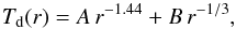 (A.1)where r is in AU and parameters A and B depend on mass and accretion luminosity:
 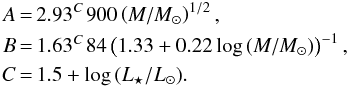 Equation (A.1) describes the temperatures induced by the central accretion energy source (ignoring ISRF), valid for Td ≲ 300 K. The first term in Eq. (A.1) approximates the steepest profiles in the inner semi-opaque region, the second term represents temperatures in the transparent outer part of the envelopes. An approximate borderline between the two regimes can be estimated directly from Fig. 3 as
 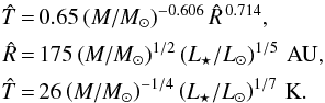 (A.2)
(A.2)
Appendix B: Rim-brightened backgrounds
 |
Fig. B.1 Background rim brightening in the spherical uniform-density embedding shells, either isothermal (left) or with the radiative-equilibrium Td(r) from the models (Sect. 2) of embedded starless cores (middle) and protostellar envelopes with L⋆ = 30 L⊙ (right). The intensity profiles on the left are labeled by the size ratios RE/R = { 30,3,1.3 } of the embedding cloud and the central cavity, whereas the intensity profiles at 500 μm in the middle and on the right indicate the mass (in M⊙) of the embedded models. For uniform temperatures (left), the brightening factors fS are 1.03,1.41, and 2.77 are the values given by Eq. (B.1). For nonuniform temperatures (and RE/R = 3, R = 104 AU), they range from 1.27 to 1.40 (middle) and from 1.44 to 1.53 (right). |
In contrast to the emission of the distant and physically unrelated backgrounds or foregrounds, embedding backgrounds resemble craters. The central spherical region occupied by an object (r ≤ R) does not belong to the embedding cloud (R<r ≤ RE) and thus must be considered empty when determining the object’s background. Rim brightening for uniform-density transparent isothermal clouds with such a cavity depends only on their relative radial thickness (RE−R) /R. It can be quantified by the ratio fS of intensities (or column densities) along the lines of sight passing through the rim and the center of the cavity:  (B.1)According to Eq. (B.1), the background under embedded objects can be overestimated from a few percent to a factor of several, hence background-subtracted values and masses may become substantially underestimated. For the present models with R = 104AU and RE/R = 3, the background and masses are over- and underestimated by fS = 1.41, respectively. The value is the discrepancy of derived masses seen for the embedded starless cores and protostellar envelopes (Figs. 6−9, D.2, D.3). The effect becomes much stronger for very thin shell-like embedding clouds, whereas it vanishes for extended background clouds. For the size ratios RE/R of 1.3 and 30, the factor fS takes the values of 2.77 and 1.03, respectively. Numerical examples of the rim-brightened backgrounds for both isothermal and non-isothermal spherical embedding clouds are shown in Fig. B.1.
Realistic temperature profiles in the embedding clouds bring only minor quantitative changes, not altering qualitatively the rim brightening effect (Fig. B.1). Steep positive or negative temperature gradients in the dense shells around embedded starless cores and protostellar envelopes (Fig. 3) tend to slightly reduce or increase the brightening effect (by ~ 10%), respectively.
Actual geometry of the real background clouds is of minor importance, the only relevant assumption is that the embedded object (hence, its background cavity) has a convex shape. For instance, assuming a plane-parallel embedding cloud with thickness 2 RE along the line of sight, it is possible to obtain a slightly different expression than Eq. (B.1) for the rim brightening factor: 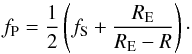 (B.2)Plane-parallel geometry makes the brightening factors fP somewhat larger than fS from Eq. (B.1), with the difference being stronger for thinner shell-like clouds. For instance, the size ratios RE/R of 30,3, and 1.3, correspond to the brightening factors fP of 1.03,1.46, and 3.55, respectively.
Depths of the background craters may be quite dissimilar for different objects in real observations. The observations show that the interstellar medium is strongly filamentary and that stars tend to form in narrow, very dense filaments (e.g., Men’shchikov et al. 2010; André et al. 2014). For an object embedded in a cylindrical filament of radius RE in the plane of the sky, the brightening factor fC is intermediate between fS and fP, depending on the position angle of the radius-vector from the center of the object to its outer boundary R. It is easy to see that fC = fP along the filament’s axis, whereas fC = fS in the orthogonal direction, across the filament.
The widths of the embedding filaments appear to be similar to the sizes of embedded objects (Men’shchikov et al. 2010). Assuming their cylindrical geometry, the embedding filaments of starless cores and protostellar envelopes are likely to have RE only a factor of about 2−3 larger than R. For such narrow filamentary backgrounds of resolved objects, the rim brightening effect is quantified by factors fC ≈ 1.8−1.4.
Background rim brightening may be observable only when imaging the nearby resolved sources unaffected by other distant back- or foregrounds. With this effect in action, the standard observational algorithm of background subtraction underestimates Fν by factors similar to fS or fP. With poorer angular resolutions, the rim of the background crater gets smeared out and thus the brightening effect eventually vanishes for unresolved sources which also have an opposite trend to produce underestimated background and hence overestimated Iν and Fν (cf. Sect. 5.2).
Appendix C: Fitting procedure
The nonlinear least-squares fitting algorithm used in this work employs the Levenberg-Marquardt method (Press et al. 1992) that minimizes χ2 residuals between the model and data. The method requires a user to provide initial guesses for model parameters. Tests have shown that an arbitrary choice of the initial values of the fitting models (Sects. 3.1, 3.2) does not guarantee convergence to the global χ2 minimum. A fully automated fitting procedure has been designed to overcome this problem and avoid any need to make arbitrary initial guesses.
The algorithm explores the multidimensional parameter space of the model with a large number of trial fittings of the spectral distributions of data points. The parameter space is discretized in logarithmically equidistant steps δlog p, covering all relevant initial values of temperature T (4−103 K), mass M (3 × 10⁻³−3 × 10²M⊙), column density NH2 (1017−1027 cm-2), and solid angle Ω (1.85 × 10⁻¹³−1.85 × 10⁻⁵ sr). Large initial discretization steps δlog p ~ 10 and the above ranges of parameters are adaptively refined in an iterative binary search down to δlog p ≈ 0.1, accelerating the algorithm in finding the global minimum. Data points are fitted using all combinations of the model parameters6 in the adaptively refined parameter space and their initial values are found that converge to the globally smallest χ2 in a fully automated procedure.
Algorithms described in this paper were written as a versatile and robust FORTRAN utility fitfluxes that efficiently estimates modbody or thinbody parameters from fitting either total fluxes of cataloged sources or intensities of multiwavelength images. The code is easy to install and use and it is freely available from the author upon request.
Appendix D: Results for isothermal models
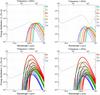 |
Fig. D.1 Spectral energy distributions of the isothermal models of starless cores (upper) and protostellar envelopes (lower). Shown are the background-subtracted fluxes of the isolated models (left) and of their embedded variants (right). For the cores of increasing masses, TM = {16.3, 15.0, 13.2, 11.2, 9.25, 7.66, 6.42 K}. For the envelopes of increasing luminosities and masses, TM = {16.6, 16.8, 17.3, 18.1, 19.5, 21.9, 25.9 K}, TM = {13.8, 14.1, 14.7, 15.6, 17.1, 19.4, 23.0 K}, TM = {10.0, 10.4, 11.1, 12.3, 14.1, 16.8, 20.7 K}. See Fig. 4 for more details. |
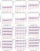 |
Fig. D.2 Masses MF derived from fitting Fν for the isothermal models of both isolated and embedded starless cores and protostellar envelopes. Compared to the results for isolated models, all derived masses of embedded models are underestimated by approximately a factor of 1.3, owing to background over-subtraction (Sect. 5.2). See Fig. D.1 for SEDs and Fig. 6 for more details. |
The importance of estimating TF that approaches the mass-averaged temperature TM from Eq. (4) for deriving accurate masses is shown by isothermal models, those described in Sect. 2 and used throughout this paper where self-consistent (radiative-equilibrium) profiles Td(r) were replaced with TM. The isothermal models were then observed and imaged in a ray-tracing run of the radiative transfer code. The resulting SEDs (Fig. D.1) are essentially the modified blackbody shapes κνBν(TM) ν and the same is true for the spectral shapes of image pixels. The temperature excesses above TM (Sect. 5.3) that greatly distorted the model SEDs (Fig. 4) towards shorter wavelengths do not exist in the isothermal models. Consequently, the isothermal shapes of Fν and Iνij bring much more expected and accurate results.
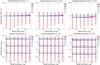 |
Fig. D.3 Masses Mℐ derived from fitting images ℐν of the isothermal models of both isolated and embedded starless cores and protostellar envelopes for the correct value of β = 2. Two columns of panels (left, middle) display the masses derived for resolved and unresolved images of the isolated models, whereas the third column of panels (right) present results for unresolved embedded models. Angular resolutions do not make any difference for the isothermal models. See Fig. D.2 and Fig. 8 for more details. |
With the correct value β = 2, derived MF of the isolated starless cores and protostellar envelopes derived with thinbody agree with the true masses M (Fig. D.2). The same results are obtained for modbody, with the exception of the minimal subset Φ3 for some models. An inspection of the problematic fits show that TF is somewhat overestimated because of an additional degree of freedom in modbody and a formal search for a globally best fit in its parameter space. The fits in question have the globally lowest χ2 value, but they correspond to small values of Ω and, therefore, to high optical depth τν ~ 1. However, there are also other very good fits with somewhat larger χ2 that do produce accurate TF = TM with τν ≪ 1, consistent with the models. The problem seems to be just a simple consequence of the finite accuracy of the numerical models and their fluxes.
With the same β = 2, the derived masses of the embedded models (Fig. D.2) are almost uniformly underestimated by a factor of approximately 1.3. The reason for the difference with respect to the isolated models is the conventional approach to background subtraction. Emission of a transparent cloud embedding a physical object tends to be rim brightened (Appendix B, Sect. 5.2). An average intensity in an annulus may overestimate background, from a few percent to a factor of several, hence may underestimate the background-subtracted intensities Iν, fluxes Fν, and derived masses (see Sects. 4.2 and 4.3).
For an inadequate fitting model, skewed by β values fixed below or above its correct value, the fits are obviously biased to over- or underestimate TF and hence to under- or overestimate MF, correspondingly (Fig. D.2). The inaccuracy is within a factor of 2, independently of whether β is a factor of 1.2 lower or higher. Fitting larger subsets Φn (n = 2 → 6) for the isothermal models may give somewhat better derived parameters, as they better constrain TF with an incorrect slope β.
Mass derivation from images ℐν of the isothermal models delivers results that are similar to those described above for both isolated and embedded variants (Fig. D.3). Dependence on the adopted β is the same as described above, hence only the results with correct β = 2 are presented. With no temperature deviations from TM in the isothermal models, derived Mℐ are very accurate for all angular resolutions, in contrast to the results with the self-consistent Td(r) (Figs. 8 and 9). Derived Mℐ for the embedded models are practically identical to MF, being underestimated by a factor of 1.3 owing to the background rim-brightening effect (Appendix B, Sect. 5.2).
Appendix E: Results for free variable β
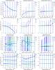 |
Fig. E.1 Temperatures TF and masses MF derived from fitting Fν of isolated, embedded, and isothermal models (fits with free variable β) for starless cores (upper) and protostellar envelopes (lower). See Fig. 6 for more details. |
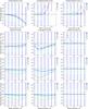 |
Fig. E.2 Opacity slope βF derived from fitting Fν of isolated, embedded, and isothermal models (fits with free variable β) for starless cores (upper) and protostellar envelopes of selected masses (3, 0.3, and 0.03 M⊙, lower). See Fig. 6 for more details. |
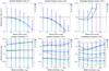 |
Fig. E.3 Masses Mℐ derived from fitting images ℐν of the isolated and embedded starless cores and protostellar envelopes (fits with free variable β). Two columns of panels (left, middle) display the masses derived for the resolved and unresolved images of the isolated models, whereas the third column of panels (right) presents results for the unresolved embedded models. Derived masses of the latter are underestimated by a factor of approximately 1.3 as a result of the conventional procedure of background subtraction (Sect. 5.2). See Fig. 8 for more details. |
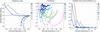 |
Fig. E.4 Relationships between TF and βF derived from fitting fluxes Fν of starless cores and protostellar envelopes (fits with free variable β). Curves plotted with squares (dark colors) and circles (bright colors) in the left and middle panels correspond to the isolated and embedded models, whereas in the right panel they correspond to the isothermal versions of the isolated starless cores and protostellar envelopes, respectively. Results for the starless cores are plotted for all masses 0.03−30 M⊙. Results for the protostellar envelopes, shown for only selected masses (0.03,0.3, and 3 M⊙, three sets of identical lines), span the entire range of luminosities 0.03−30 L⊙. Thick horizontal lines indicate the true value β = 2. For clarity of the plots, error bars are not shown. |
In some applications of the mass derivation methods, the opacity slope β has been allowed to vary along with the other fitting parameters (T, M, Ω). To quantify effects of the extra degree of freedom, additional fits with variable β were performed in this study. Although the parameters for both fitting models were derived and analyzed, only the much less incorrect thinbody results are presented and discussed here.
Figure E.1 compares derived TF and MF of the isolated, embedded, and isothermal variants of starless cores and protostellar envelopes with the true model values (TM, M). Although the isolated cores and envelopes display behavior that is qualitatively similar to the β = 2 case (Sect. 4.2), the biases in TF and MF towards denser (more massive) cores and envelopes, as well as over L⋆ for the latter, become much stronger. For example, for the isolated starless cores with M ≳ 10 M⊙, derived TF are overestimated by a factor of 2, whereas MF are underestimated by a factor of 15. For the embedded protostellar envelopes of M = 3 M⊙ with L⋆ ≲ 1 L⊙, temperatures are overestimated by a similarly large factor and MF underestimated by a factor of 8.
Such errors are caused by the derived βF whose values for starless cores are systematically lowered towards higher mass models, and are underestimated by a factor of 4 (Fig. E.2). In the case of the embedded protostellar envelopes, the values of βF are progressively underestimated towards lower luminosities, up to a factor of 2 (Fig. E.2). The very large errors in βF are, in turn, caused by the temperature excesses over TM (Sect. 5.3), which is highlighted in Fig. E.1 by the accurate results for the isothermal models. As in the fixed β case, errors in derived parameters for the embedded starless cores are smaller than those for the isolated cores, whereas the behavior is opposite for the embedded protostellar envelopes (cf. Figs. 6, 7). However, the biases over the masses and luminosities in Fig. E.1 become stronger than in the fixed β case, which again is attributed to the additional biases in the derived βF values (Fig. E.2).
The method of fitting images ℐν delivers results that are similar to those described above, for both isolated and embedded variants (Fig. E.3) of partially resolved and unresolved objects. Derived masses for the fully resolved objects are much more accurate and they do not depend on the subset of data points Φn, for the reasons discussed in Sects. 4.3 and 5.1. With degrading angular resolutions, accuracy of the estimated parameters deteriorates to the levels obtained from the method of fitting total fluxes Fν (Fig. E.1). Larger beams heavily blend emission with nonuniform temperatures from different pixels, distorting their spectral distribution towards shorter wavelengths. In both methods, derived masses become systematically much less accurate (greatly underestimated) when fitting larger subsets Φn (n = 3 → 6). However, even the smallest subsets Φ3 show very significant inaccuracies and different biases that depend on the mass and luminosity of an object.
The above results obtained with free fitting parameter β can be compared with those from the previous studies focused on the relationship between derived temperature and opacity slope (cf. Shetty et al. 2009a,b; Juvela & Ysard 2012, and references therein). Figure E.4 shows the intrinsic dependencies between βF and TF for the isolated and embedded starless cores and protostellar envelopes, and for the isothermal versions of the isolated models. The correlations between βF and TF take variety of shapes, from a strongly positive to a strongly negative correlation, with practically no correlation for the isothermal models. This suggests that they must be caused by different kinds of deviations of the spectral shapes of Fν (Fig. 4) produced by the nonuniform Td(r) (Fig. 3) from Fν(TM) (Fig. D.1). Smaller subsets Φn (n = 6 → 3) bring less correlated βF and TF than the large subsets do. For the protostellar envelopes, the correlations are non-monotonic and they may either be strongly negative or positive, depending on the luminosity of the central energy source.
All Figures
|
Fig. 1 Opacities of grains (per gram of dust) and model radial optical depths. Subscripts on the curve labels (n30 to n0.03) indicate the model mass M (in M⊙). The wavelength dependence of κsca, κabs, and κext is shown by thick solid lines (see Sect. 2.1 for details). The extinction optical depths τext of the protostellar envelopes (L⋆ = 0.3 L⊙) and starless cores are indicated respectively by the three sets of dashed blue and red lines. |
| In the text | |
|
Fig. 2 Density structure of the model starless cores and protostellar envelopes. Subscripts on the curve labels (n30 to n0.03) indicate the model mass M (in M⊙). The dashed vertical line shows the outer boundary radius R = 104 AU for all models. Embedded models are implanted in larger uniform-density clouds with an outer boundary at 3 × 10⁴ AU. The dashed horizontal lines continue the densities of starless cores within the innermost radial zone. The dashed diagonal lines continue the densities of protostellar envelopes towards the radius of the inner dust-free cavity R0, whose size depends on the model temperature profile Td(r) (cf. Fig. 3) and adopted dust sublimation temperature (TS = 103 K). In other words, the dashed diagonal lines visualize the range of densities and radial distances over which the inner boundary R0 is located for L⋆ spanning the entire range 0.03 − 30 L⊙ (see Eq. (1)). |
| In the text | |
|
Fig. 3 Radiative-equilibrium dust temperature profiles of starless cores (upper) and protostellar envelopes (lower) for the isolated models (left) and their embedded variants (right). Subscripts of the curve labels (T30 to T0.03) indicate the model mass M (in M⊙). The dashed horizontal lines in the upper panels continue the profiles of starless cores within the innermost radial zone. The dashed vertical line shows the outer boundary radius R = 104 AU of all models. The maximum temperature and the inner boundary of the dusty protostellar envelopes are defined by the adopted dust sublimation temperature TS = 103 K. Three dashed horizontal lines in the lower panels indicate the range of radial distances over which the boundaries R0 of the dust-free cavities are located for the model luminosities in the entire range of 0.03 − 30 L⊙ (see Fig. 2). For protostellar envelopes with the same M, the “hotter” profiles correspond to higher L⋆, larger R0 (cf. Eq. (1)), and lower radial optical depths |
| In the text | |
|
Fig. 4 Spectral energy distributions starless cores (upper) and protostellar envelopes (lower). Shown are the background-subtracted fluxes for the isolated models (left) and their embedded variants (right). Subscripts of the curve labels (F30 to F0.03) indicate the model mass (in M⊙). For protostellar envelopes of the same mass, the SEDs with higher fluxes correspond to higher accretion luminosities L⋆ (0.03, 0.1, 0.3, 1, 3, 10, 30 L⊙). Dashed lines indicate the fluxes of the ISRF that were integrated over the projected area of either the isolated models or the embedding clouds. |
| In the text | |
|
Fig. 5 Fluxes of the isolated starless cores (upper) and protostellar envelopes (lower) fitted with the thinbody (left) and modbody (right) models. The fluxes for the 0.03, 0.3, and 3 M⊙ cores and envelopes (with L⋆ = 1 L⊙) from Fig. 4 are shown as black triangles, squares, and circles, respectively. Successful fits (Sect. 3.4) using different subsets Φn of fluxes are indicated by the solid and dashed lines of different widths and colors. The thin black curves show the flux distributions for the isothermal models where the actual model temperatures (Fig. 3) were replaced with their mass-averaged values: Td(r) = TM (16.3,13.2,9.2 K for starless cores and 18.1,15.6,12.3 K for protostellar envelopes). |
| In the text | |
|
Fig. 6 Temperatures TF and masses MF derived from fitting Fν of both isolated and embedded starless cores vs. the true model values of TM and M for three β values (1.67, 2, 2.4). For various subsets Φn of fluxes, results from successful thinbody and modbody fits (Sect. 3.4) are displayed by the colored and gray lines, respectively. Error bars represent the 1 × σ uncertainties of the derived parameters returned by the fitting routine combined with the assumed ± 20% uncertainties of η, κ0, and D (Sect. 3.4). The black solid lines show the locations where TF and MF are equal to the true values. To preserve clarity of the plots, much less accurate modbody results are displayed only for correct β = 2 and without error bars. |
| In the text | |
|
Fig. 7 Temperatures TF and masses MF derived from fitting Fν of both isolated and embedded protostellar envelopes (with the true masses M of 0.03, 0.3, and 3M⊙) vs. the true model values of TM and L for three β values (1.67, 2, 2.4). Results from successful thinbody and modbody fits for various subsets Φn of fluxes (Sect. 3.4) are displayed by the colored and gray lines, respectively. See Fig. 6 for more details. |
| In the text | |
|
Fig. 8 Temperatures Tℐ and masses Mℐ derived from fitting images ℐν of both isolated and embedded starless cores vs. the true model values of TM and M for correct β = 2. The three columns of panels present results for three angular resolutions (resolved, partially resolved, and unresolved cases) and for various subsets Φn of pixel intensities. Error bars represent the 1 × σ uncertainties of the derived Tℐ and Mℐ (computed over all pixels as the NH2-averaged errors of TNij and integrated errors of NH2, correspondingly), combined with the assumed ± 20% uncertainties of η, κ0, and D (Sect. 3.4). Less reliable results (n−γ + 1 <χ2< 10 in some pixels) are shown without error bars. See Fig. 6 for more details. |
| In the text | |
|
Fig. 9 Temperatures Tℐ and masses Mℐ derived from fitting images ℐν of both isolated and embedded protostellar envelopes (with the true masses M of 0.03,0.3, and 3 M⊙) vs. the true model values of TM and L for correct β = 2. The three columns of panels present results for three angular resolutions indicated (resolved, partially resolved, and unresolved cases). See Fig. 8 for more details. |
| In the text | |
|
Fig. B.1 Background rim brightening in the spherical uniform-density embedding shells, either isothermal (left) or with the radiative-equilibrium Td(r) from the models (Sect. 2) of embedded starless cores (middle) and protostellar envelopes with L⋆ = 30 L⊙ (right). The intensity profiles on the left are labeled by the size ratios RE/R = { 30,3,1.3 } of the embedding cloud and the central cavity, whereas the intensity profiles at 500 μm in the middle and on the right indicate the mass (in M⊙) of the embedded models. For uniform temperatures (left), the brightening factors fS are 1.03,1.41, and 2.77 are the values given by Eq. (B.1). For nonuniform temperatures (and RE/R = 3, R = 104 AU), they range from 1.27 to 1.40 (middle) and from 1.44 to 1.53 (right). |
| In the text | |
|
Fig. D.1 Spectral energy distributions of the isothermal models of starless cores (upper) and protostellar envelopes (lower). Shown are the background-subtracted fluxes of the isolated models (left) and of their embedded variants (right). For the cores of increasing masses, TM = {16.3, 15.0, 13.2, 11.2, 9.25, 7.66, 6.42 K}. For the envelopes of increasing luminosities and masses, TM = {16.6, 16.8, 17.3, 18.1, 19.5, 21.9, 25.9 K}, TM = {13.8, 14.1, 14.7, 15.6, 17.1, 19.4, 23.0 K}, TM = {10.0, 10.4, 11.1, 12.3, 14.1, 16.8, 20.7 K}. See Fig. 4 for more details. |
| In the text | |
|
Fig. D.2 Masses MF derived from fitting Fν for the isothermal models of both isolated and embedded starless cores and protostellar envelopes. Compared to the results for isolated models, all derived masses of embedded models are underestimated by approximately a factor of 1.3, owing to background over-subtraction (Sect. 5.2). See Fig. D.1 for SEDs and Fig. 6 for more details. |
| In the text | |
|
Fig. D.3 Masses Mℐ derived from fitting images ℐν of the isothermal models of both isolated and embedded starless cores and protostellar envelopes for the correct value of β = 2. Two columns of panels (left, middle) display the masses derived for resolved and unresolved images of the isolated models, whereas the third column of panels (right) present results for unresolved embedded models. Angular resolutions do not make any difference for the isothermal models. See Fig. D.2 and Fig. 8 for more details. |
| In the text | |
|
Fig. E.1 Temperatures TF and masses MF derived from fitting Fν of isolated, embedded, and isothermal models (fits with free variable β) for starless cores (upper) and protostellar envelopes (lower). See Fig. 6 for more details. |
| In the text | |
|
Fig. E.2 Opacity slope βF derived from fitting Fν of isolated, embedded, and isothermal models (fits with free variable β) for starless cores (upper) and protostellar envelopes of selected masses (3, 0.3, and 0.03 M⊙, lower). See Fig. 6 for more details. |
| In the text | |
|
Fig. E.3 Masses Mℐ derived from fitting images ℐν of the isolated and embedded starless cores and protostellar envelopes (fits with free variable β). Two columns of panels (left, middle) display the masses derived for the resolved and unresolved images of the isolated models, whereas the third column of panels (right) presents results for the unresolved embedded models. Derived masses of the latter are underestimated by a factor of approximately 1.3 as a result of the conventional procedure of background subtraction (Sect. 5.2). See Fig. 8 for more details. |
| In the text | |
|
Fig. E.4 Relationships between TF and βF derived from fitting fluxes Fν of starless cores and protostellar envelopes (fits with free variable β). Curves plotted with squares (dark colors) and circles (bright colors) in the left and middle panels correspond to the isolated and embedded models, whereas in the right panel they correspond to the isothermal versions of the isolated starless cores and protostellar envelopes, respectively. Results for the starless cores are plotted for all masses 0.03−30 M⊙. Results for the protostellar envelopes, shown for only selected masses (0.03,0.3, and 3 M⊙, three sets of identical lines), span the entire range of luminosities 0.03−30 L⊙. Thick horizontal lines indicate the true value β = 2. For clarity of the plots, error bars are not shown. |
| In the text | |
Current usage metrics show cumulative count of Article Views (full-text article views including HTML views, PDF and ePub downloads, according to the available data) and Abstracts Views on Vision4Press platform.
Data correspond to usage on the plateform after 2015. The current usage metrics is available 48-96 hours after online publication and is updated daily on week days.
Initial download of the metrics may take a while.