| Issue |
A&A
Volume 592, August 2016
|
|
|---|---|---|
| Article Number | A105 | |
| Number of page(s) | 31 | |
| Section | Extragalactic astronomy | |
| DOI | https://doi.org/10.1051/0004-6361/201527179 | |
| Published online | 08 August 2016 | |
First survey of Wolf-Rayet star populations over the full extension of nearby galaxies observed with CALIFA⋆
1 Departamento de Física Teórica, Universidad Autónoma de Madrid, 28049 Madrid, Spain
e-mail: This email address is being protected from spambots. You need JavaScript enabled to view it.
2 Sydney Institute for Astronomy, School of Physics A28, University of Sydney, NSW 2006, Australia
3 Australian Astronomical Observatory, PO BOX 296, Epping, NSW 1710, Australia
4 Instituto Nacional de Astrofísica, Óptica y Electrónica, Luis E. Erro 1, 72840 Tonantzintla, Puebla, Mexico
5 GEPI, Observatoire de Paris, CNRS, Université Paris-Diderot, Place Jules Janssen, 92190 Meudon, France
6 Instituto de Astrofísica de Andalucía (CSIC), Glorieta de la Astronomía s/n, Aptdo. 3004 18080 Granada, Spain
7 Instituto de Astronomí a,Universidad Nacional Autonóma de Mexico, A.P. 70-264, 04510 México, D.F., Mexico
8 Leibniz-Institut für Astrophysik Potsdam (AIP), An der Sternwarte 16, 14482 Potsdam, Germany
9 Millennium Institute of Astrophysics MAS, Nuncio Monseñor Sótero Sanz 100, Providencia, 7500011 Santiago, Chile
10 Departamento de Astronomía, Universidad de Chile, Camino El Observatorio 1515, Las Condes, Santiago, Chile
11 Max Planck Institute for Astronomy, Königstuhl 17, 69117 Heidelberg, Germany
12 Instituto de Astrofísica de Canarias (IAC), 38205 La Laguna, Tenerife, Spain
13 Centro de Astrofísica and Faculdade de Ciencias, Universidade do Porto, Rua das Estrelas, 4150-762 Porto, Portugal
14 Centro Astronómico Hispano Alemán, Calar Alto, (CSIC-MPG), C/Jesús Durbán Remón 2-2, 04004 Almería, Spain
Received: 12 August 2015
Accepted: 10 May 2016
Abstract
The search of extragalactic regions with conspicuous presence of Wolf-Rayet (WR) stars outside the Local Group is challenging task owing to the difficulty in detecting their faint spectral features. In this exploratory work, we develop a methodology to perform an automated search of WR signatures through a pixel-by-pixel analysis of integral field spectroscopy (IFS) data belonging to the Calar Alto Legacy Integral Field Area survey, CALIFA. This procedure has been applied to a sample of nearby galaxies spanning a wide range of physical, morphological, and environmental properties. This technique allowed us to build the first catalogue of regions rich in WR stars with spatially resolved information, and enabled us to study the properties of these complexes in a two-dimensional (2D) context. The detection technique is based on the identification of the blue WR bump (around He iiλ4686 Å, mainly associated with nitrogen-rich WR stars; WN) and the red WR bump (around C ivλ5808 Å, mainly associated with carbon-rich WR stars; WC) using a pixel-by-pixel analysis that maximizes the number of independent regions within a given galaxy. We identified 44 WR-rich regions with blue bumps distributed in 25 out of a total of 558 galaxies. The red WR bump was identified only in 5 of those regions. Most of the WR regions are located within one effective radius from the galaxy centre, and around one-third are located within ~1 kpc or less from the centre. We found that the majority of the galaxies hosting WR populations in our sample are involved in some kind of interaction process. Half of the host galaxies share some properties with gamma-ray burst (GRB) hosts where WR stars, such as potential candidates to the progenitors of GRBs, are found. We also compared the WR properties derived from the CALIFA data with stellar population synthesis models, and confirm that simple star models are generally not able to reproduce the observations. We conclude that other effects, such as binary star channel (which could extend theWR phase up to 10 Myr), fast rotation, or other physical processes that cause the loss of observed Lyman continuum photons, very likely affect the derived WR properties, and hence should be considered when modelling the evolution of massive stars.
Key words: galaxies: starburst / galaxies: ISM / stars: Wolf-Rayet / techniques: imaging spectroscopy
Based on observations collected at the Centro Astronómico Hispano-Alemán (CAHA) at Calar Alto, operated jointly by the Max-Planck Institut für Astronomie and the Instituto de Astrofísica de Andalucía (CSIC).
© ESO, 2016
1. Introduction
Despite their relatively low numbers, massive stars dominate the stellar feedback to the local interstellar medium (ISM) through their stellar winds and subsequent death as supernovae (SNe). The most massive stars (M ≥ 25M⊙ for Z⊙) undergo the Wolf-Rayet (WR) phase starting 2–3 Myr after their birth (Meynet 1995). These stars have typical wind densities that are an order of magnitude higher than massive O stars, and hence play a key role in the chemical enrichment of galaxies. Although WR stars evade direct detection, they are likely to be the progenitors of Type Ib and Type Ic core-collapse SNe, which are likely to be linked to ongoing star formation (Galbany et al. 2014). These SN types are characterized by showing neither hydrogen (SNIb) nor helium (SNIc) in their spectra, suggesting that the external layers of the progenitor star were removed prior to explosion. Moreover, a small fraction of SNe Ic showing broad-line features in the spectra (SNIc-bl; ~30 000 km s-1) are associated with long-duration gamma-ray bursts (GRBs; Galama et al. 1998; Stanek et al. 2003; Hjorth et al. 2003; Modjaz et al. 2006). Indeed, it has been suggested that WR stars are candidate progenitors of long, soft GRBs in regions of low metallicity (Woosley & Heger 2006).
The emission features that characterize the spectra of WR stars are often observed in extragalactic H ii regions. WR winds are sufficiently dense that an optical depth of unity in the continuum arises in the outflowing material. The spectral features are formed far out in the wind and are seen primarily in emission (Crowther 2007). Generally WR stars are identified in galaxies (first renamed “WR galaxies” by Osterbrock & Cohen 1982) whenever their integrated spectra show a broad He ii emission feature centred at 4686 Å, the so-called blue WR bump. Some few other broad features, such as the red WR bump around C ivλ5808, are also used to identify WR stars in galaxies, but these features are in most cases much fainter than the blue WR bump. In any case, the term “WR galaxy” may be confusing. Depending on the distance to the observed galaxy and the spatial resolution and extension of the extracted spectrum, it may well refer to extragalactic H ii regions and very frequently to the nucleus of a powerful starburst. Galaxies showing a significant population of WR stars have been known for several decades, beginning with the first WR detection in the blue compact dwarf galaxy He 2-10 (Allen et al. 1976). Since then a number of the WR galaxies have been reported, although generally through a serendipitous detection (e.g. Kunth & Sargent 1981, 1983; Ho et al. 1995; Heckman et al. 1997).
The investigation of the WR content in galaxies provides important constrains to stellar evolutionary models. This is particularly important at low metallicities because very little data of subsolar WR stars are available. Several studies have attempted to reproduce the number of WR stars needed to account for the observed stellar emission features. The disagreement between observations and models concerning simple calculations, such as the flux ratio between the blue WR bump and Hβ or the WR/O number ratio at subsolar metallicities (which is a sensitive test of evolutionary models), has lead to the development of sophisticated models that include rotation (Meynet & Maeder 2005) or binary evolution of massive stars (Van Bever & Vanbeveren 2003; van Bever & Vanbeveren 2007; Eldridge et al. 2008). Therefore, studies of large samples of galaxies showing WR features, especially in the intermediate- and low-metallicity regime, are needed to better constrain such models.
Ideally, detailed, spatially resolved studies of WR populations would be needed to fill the gap between early detailed works and large surveys of integrated properties. Several studies in nearby starbursts (e.g. Gonzalez-Delgado et al. 1994; Pérez-Montero & Díaz 2007; Pérez-Montero et al. 2010; López-Sánchez & Esteban 2010; Karthick et al. 2014) and resolved knots of star formation (e.g. Gonzalez-Delgado et al. 1995; Castellanos et al. 2002; Hadfield & Crowther 2006) have been published during the last few years in conjunction with studies of individual WR stars in galaxies of the Local Group (e.g. Massey & Hunter 1998; Massey 2003; Crowther & Hadfield 2006; Crowther et al. 2006; Neugent et al. 2012; Hainich et al. 2014; Sander et al. 2014). However, spatially resolved and detailed studies of extragalactic regions showing a significant WR population in large galaxy samples have not been accomplished yet.
The advent of the integral field spectroscopy (IFS) allows us to obtain simultaneously both spectral and spatial information of galaxies. Therefore, IFS techniques provide a more efficient way to study the spatial distribution of the WR population in nearby galaxies. Indeed, such studies have been conducted in some individual galaxies (e.g. James et al. 2009; López-Sánchez et al. 2011; Monreal-Ibero et al. 2013; Kehrig et al. 2013). In particular, Miralles-Caballero et al. (2014b; henceforth, MC14b) used data from the PPAK Integral Field Spectroscopy (IFS) Nearby Galaxies Survey (PINGS; Rosales-Ortega et al. 2010) to locate the WR-rich regions in the nearby spiral galaxy NGC 3310. PINGS was specifically designed to study the spatially resolved properties of a sample of 17 nearby spiral galaxies. Among the almost 100 H ii regions identified throughout the disc of NGC 3310 by Miralles-Caballero et al. (2014a), MC14b reported the detection of WR features in 18 of these regions. The methodology developed by MC14b using IFS data mitigates aperture effects and allows us to spatially resolve the emission of the WR population in local galaxies (Kehrig et al. 2013). Indeed, their technique can be applied to large galaxy samples. Also, IFS observations provide powerful tools to minimize the WR bump dilution and find WR stars in extragalactic H ii regions where they were not detected before (Kehrig et al. 2008; Cairós et al. 2010; García-Benito et al. 2010; Monreal-Ibero et al. 2010, 2012; Perez-Montero et al. 2013). In addition, spatially resolved studies can also be used to explore the connection between the environment and the WR emission. The study of the environment is of particular interest to get clues about the connection between WR stars and SNIc-bl/GRBs, since these massive stars may actually be progenitors of these explosions. Although a direct link between GRBs to WR stars cannot be made, it is possible to compare the properties of GRB host galaxies with those of WR stars and indirectly obtain information on the GRB progenitors in this way. Kelly et al. (2008), expanding the work by Fruchter et al. (2006), showed that both SNIc-bl and GRB tend to occur in the brightest regions of their host galaxies. Leloudas et al. (2010) correlated the locations of WR stars with GRBs and different SN types, finding that SNe Ibc and WR showed a high degree of association and that the connection between WR and GRBs could not be excluded. Some other studies have reported that the host galaxies of nearby GRB often host WR stars too, although the WR-rich areas do not necessarily coincide with the location of the GRBs (Cerviño 1998; Hammer et al. 2006; Christensen et al. 2008; Han et al. 2010; Levesque et al. 2011; Thöne et al. 2014). Therefore, studies of WR galaxies and their relation with their environment may also provide insight into the properties of GRB progenitors.
Previous searches for WR regions across individual galaxies outside the Local Group have been performed, for example in NGC 300 (Schild et al. 2003), M83 (Hadfield et al. 2005), NGC 1313 (Hadfield & Crowther 2007), NGC 7793 (Bibby & Crowther 2010), NGC 5068 (Bibby & Crowther 2012), and M101 (Shara et al. 2013). Currently, a systematic search for the spatially resolved WR populations in a sample of nearby galaxies can be performed with the aid of IFS. Examples include Brinchmann et al. (2008a; henceforth, B08a), and Shirazi & Brinchmann (2012) who accomplished the task by analysing a few hundred thousand spectra obtained with fibres. In this work we analyse a sample of 558 galaxies observed with IFS to compile a homogeneous catalogue of galaxies showing regions with WR populations for the first time.
Galaxies of all different environments were considered, i.e. isolated galaxies, compact dwarf galaxies, and targets showing past signs of recent and ongoing interactions. We were able to identify resolved Hα clumps in the galaxies thanks to the two-dimensional (2D) coverage of IFS data, and thus avoid restricting the search of WR-rich areas to only the brightest H ii complexes, as is usually imposed in other studies. The main goal of this article is to relate, for the first time, the WR populations in this homogeneous galaxies sample with their spatially resolved properties to explore the influence of morphology in the recurrence of these features, and to study the effect of binarity, photon leakage, and metallicity in the observed properties of WR emission lines in the Local Universe.
The paper is organized as follows: Sect. 2 presents our IFS galaxy sample and gives some details about the data reduction process. In Sect. 3, we then describe the methodology used to pinpoint regions showing WR emission using data from IFS surveys. Section 4 presents our catalogue of regions showing WR emission features. Here we outline the overall properties of the host galaxies and describe the procedure to measure the different components of WR features. These measurements are later used to estimate the number of WR stars in each region. In Sect. 5 we discuss the influence of the environment and the GRB-WR connection, quantifying the effect of the dilution of the WR features when integrating over larger apertures than the observed spatial extent of the WR population, and comparing our observations with the predictions provided by synthesis stellar models. Finally, we present our conclusions in Sect. 6.
2. Initial sample and data reduction
The galaxies of this study were mainly selected from the Calar Alto Legacy Integral Field Area survey (CALIFA Sánchez et al. 2012a), which is an ongoing exploration of the spatially resolved spectroscopic properties of galaxies in the Local Universe (z< 0.03) using wide-field IFS. The CALIFA suvey observations cover the full optical extent (up to ~3−4 effective radii) of around 600 galaxies of any morphological type and are distributed across the entire colour-magnitude diagram Walcher et al. (2014). Observations were carried out using the Potsdam MultiAperture Spectrophotometer (Roth et al. 2005), mounted at the Calar Alto 3.5 m telescope, in the PPAK configuration (Kelz et al. 2006). The observations cover a hexagonal field of view (FoV) of 74′′ × 64′′, which allows us to map the full optical extent of the galaxies up to two to three effective radii. A dithering scheme of three pointings was adopted in order to cover the complete FoV and properly sample the point spread function (PSF). The observing details, selection of the galaxy sample, observational strategy, and reduction processes are thoroughly explained in Sánchez et al. (2012a) and Walcher et al. (2014). Recently, CALIFA has launched its second data release DR21, which is a set of fully reduced, quality tested and scientifically useful data cubes for 200 galaxies (García-Benito et al. 2015).
For the purpose of our study, we used 448 galaxies from the CALIFA survey observed by April 2014 in the V500 spectral set-up, which has a nominal resolution of λ/ Δλ ~ 850 at 5000 Å and a nominal wavelength range of 3749−7300 Å. The dataset was reduced using the version 1.5 of the CALIFA pipeline (García-Benito et al. 2015). The usual reduction tasks per pointing include cosmic ray rejection, optimal extraction, flexure correction, wavelength and flux calibration, and sky subtraction. Finally, all three pointings are combined to reconstruct a spatially 1″ × 1″ re-sampled data cube, which includes science data, propagated error vectors, masks, and weighting factors (see Sánchez et al. 2012a; and Husemann et al. 2013, for more details). The average value of the PSF of the datacubes is around 2.5″ (García-Benito et al. 2015). In addition, 110 galaxies from the CALIFA-Extension programmes were also included as part of our data. The CALIFA-Extension sample consists of galaxies that are not included in the main CALIFA sample and are part of specific science programmes using the same observing set-up as CALIFA. This sample includes interactive, merging, and low-mass galaxies (classes S0, Sb and dwarfs) and provides a complement to the main sample since CALIFA becomes incomplete below Mr> −19 mag, which corresponds to a stellar mass of ~109.5 M⊙ .
With a redshift range of 0.005 <z< 0.03 and absolute magnitudes above Mz = −16, the sample is representative of the galaxy population in the Local Universe (Walcher et al. 2014). Note that this sample is not purposely selected to detect as many WR features as possible, given that these populations can only be found when young ionizing stellar populations exist (i.e. typically within the first million years after they are born). Yet, this is up to now the largest sample of galaxies observed using a wide FoV (>1 arcmin2) IFS. It contains hundreds of star-forming objects (including spiral, barred, irregular and merging galaxies as well as blue compact dwarfs), and it is expected to host a significant number of regions in which populations of WR stars can be detected. With these data we can resolve regions larger than about 100 pc in radius in the closest galaxies and larger than about 600 pc in the furthest systems. These sizes are typical for giant extragalactic H ii regions and H ii complexes (Kennicutt 1984; González Delgado & Pérez 1997; Youngblood & Hunter 1999; Hunt & Hirashita 2009; Lopez et al. 2011; Miralles-Caballero et al. 2011).
3. Identification of WR features in IFS surveys
Wolf-Rayet stars have been typically discovered via techniques sensitive to their unusually broad emission-line spectra. As mentioned before, the most prominent WR emission feature observed in optical spectra corresponds to the blue bump, which is a blend of a broad He ii line at 4686 Å, nitrogen, and carbon emission lines formed in the expanding atmospheres of WR stars, and several high-excitation emission lines (sometimes including a narrow He ii line) covering the spectral range 4600−4700 Å (Schaerer & Vacca 1998). The blue WR bump, however, is generally very faint, as its flux is usually only a few percent of the flux of the Hβ emission line. The red WR bump centred around 5808 Å is usually even fainter than the blue WR bump. Therefore, a systematic search for signatures of WR emission is intrinsically challenging.
Early studies relied on the use of imaging with a narrowband λ4686 filter to detect, with great effort, the spatially resolved emission of several WRs in very nearby low-mass galaxies (Drissen et al. 1990, 1993a,b; Sargent & Filippenko 1991). Very detailed studies, in most cases even for individual stars, have been accomplished using the catalogues reported in these studies (e.g. Abbott et al. 2004; Drissen et al. 2008; Úbeda & Drissen 2009). At farther distances, faint WR signatures were detected via the analysis of integrated spectra obtained using optical fibres or long slits (e.g. Kunth & Joubert 1985; Vacca & Conti 1992; Izotov et al. 1997). These studies enabled the compilation of a few catalogues of 40–140 WR galaxies (Conti 1991; Schaerer et al. 1999; Guseva et al. 2000). The most recent surveys of WR galaxies have used single-fibre spectra from the Sloan Digital Sky Survey (SDSS2). The catalogue compiled by B08a reported 570 new WR galaxies using SDSS, and Shirazi & Brinchmann (2012) later added 189 new WR galaxies. These catalogues are limited to the size of the fibre (3′′) and, hence, they are not able to spatially resolve the WR population. Besides that, galaxies observed by SDSS show a very broad distribution of distances, sampling very heterogeneous sizes and apertures. For this study, we first focused the effort on the detection of the blue bump in our search for WR spectral signatures. Once we developed the technique we used it to detect the red bump, as explained below.
3.1. Identification of regions with the blue WR bump
Since only very massive stars (Mini> 25 M⊙ for Z⊙ ) undergo the WR phase, typically 2−3 Myr after their birth (Meynet 1995), the first natural place to search for the WR emission is where the H ii regions are located. Given that most of the stars in a cluster do not undergo this phase, however, the location of the WR stars can be restricted to a fraction of the total area of the H ii region. This effect was noticed by Kehrig et al. (2013; see Figs. 5 and 6), and, thus, our approach relies on performing a pixel-by-pixel analysis of the spectra3. The procedure followed to detect WR signatures in our galaxy sample is described as follows:
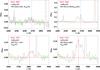 |
Fig. 1 Top: examples of continuum-subtracted spectra for a given pixel in NGC 3991 and NGC 3381 around the blue WR bump spectral range. The blue vertical line shows the location of the He iiλ4686 emission line. The spatial coordinates of the pixels (x and y) and the P/C, ϵ, and PWR parameters defined in the text are given on the left-top corner of each panel. A red continuous line indicates a linear fit to the continuum (which ideally should be an horizontal line at y = 0). The green sections of the spectrum correspond to those spectral ranges used to compute the rms. Bottom: examples of continuum-subtracted spectra for a given pixel in NGC 3773 around the red WR bump spectral range. The red vertical line indicates the location of the C ivλ5808 emission line. The coordinates of the pixels and their associated parameters are also given on the left-top corner. In both the blue and the red WR bump cases one spectrum at the limit of the detection level (left) and another with a very good detection level (right) are shown. The flux density is given in units of 10-16 erg s-1 cm-2 Å-1. |
- 1.
The first step consists in subtracting the underlying stellar population using the STARLIGHT code (Cid Fernandes et al. 2004, 2005) in order to better characterize the continuum and therefore better observe the faint WR features. It is important to note that by construction, the substraction of the underlying continuum refers to the large-scale galaxy stellar content, not including young stars cluster populations and their likely emission. A reduced spectral library set of 18 populations (3, 63, 400, 750, 2000, and 12 000 Myr, combined with Z⊙ , Z⊙ /2.5, and Z⊙ /5 metallicities) is used, so as to deal with the large amount of pixels that had to be analysed in a reasonable amount of time. These models were selected from the compilation by González Delgado et al. (2005) and the MILES library (Vazdekis et al. 2010, as updated by Falcón-Barroso et al. 2011).
- 2.
As only massive, young ionizing stars are able to undergo the WR phase, we focused only on those pixels whose approximate Hα equivalent width, EW (Hα ), is of the order of 6 Å or higher (Cid Fernandes et al. 2011; Sánchez et al. 2014). Given that the widths of the nebular lines are rather similar for the whole sample (σ ~ 2.8 Å, with no presence of emission from an AGN or other broader components), and assuming a Gaussian fit, we can roughly estimate EW (Hα ) just by measuring the observed peak of the Hα emission over the continuum (≡P/C). Under these assumptions, P / C > 0.85 practically ensures that we are dealing with a young ionizing population.
- 3.
Next, using a similar approach to that discussed in B08a, which simulates early studies that used narrowband images (e.g. Drissen et al. 1990, 1993a,b; Sargent & Filippenko 1991), we define a pseudo-filter spanning the 4600−4700 Å rest-frame range. For each pixel, we integrate the density flux, Fbump, within this spectral range and compare it with the rms in two spectral windows, 4500−4600 Å and 4750−4825 Å. We then define the detection significance, ε, as (Tresse et al. 1999)
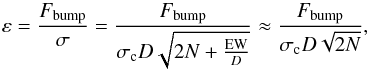 (1)where σc is the mean standard deviation per spectral point on the continuum on each side of the bump feature, D denotes the spectral dispersion in Å per spectral point, N corresponds to the number of spectral points used in the integration of the flux density, and EW refers to the equivalent width of the bump. Since EWs as low as just a few Å are expected, we neglect its contribution in the equation. After performing several visual inspections, we set the procedure to select only those spaxels with ε> 4.
 - 4.
Wolf-Rayet features are broad and have different shapes because the velocity structure of the WR winds changes between different WR stars, varying the appearance of the features significantly. The best approach to build up a reliable technique to detect WR features therefore is to construct a training set, in which WR features are clearly visible and the numerical values of detection parameters can be tested. We constructed such a training set by visual inspection of a set of spectra with tentative detections. We used the parameter PWR, which is the peak value within the WR filter range normalized to the rms. We selected those pixels with P
 . In a few cases, practically a pure narrow emission (i.e. with a width similar to that of Hβ ) is observed, and is identified as a narrow He iiλ4686 emission line. It is still not clear whether this narrow feature is intimately linked with the appearance of hot WR stars (Schaerer & Vacca 1998; Crowther & Hadfield 2006) or to O stars at low metallicities (Kudritzki 2002). We thus additionally impose
  to avoid such cases.
 - 5.
Finally, a plausible detection should occupy an area similar or larger than the CALIFA PSF. Therefore, we imposed a minimum of nine adjacent spatial elements satisfying the previous criteria to declare a positive detection. This corresponds roughly to the size of the PPAK PSF according to García-Benito et al. (2015).
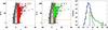 |
Fig. 2 Left: density plot (grey scale) of P/C vs. ε parameters for all the pixels in the sample for which P/C > 0.85. Contours that contain 68% (1σ), 95% (2σ) and 99% (3σ) of the points are overplotted. Red dots correspond to the values of the pre-selected regions, i.e. before imposing the grouping of at least 9 pixels. Middle: same as before, but this time the overplotted green dots correspond to selected regions, also obeying the grouping criterion. The orange vertical line indicates the cut used for ε (4), while the horizontal line denotes P/C ~ 2.1 parameter, having practically all the selected pixels a higher value than this limit. Right: histogram of ε for pixels with P/C > 0.85 (black), pre-selected pixels (red), selected pixels (green), and for those pre-selected pixels not satisfying the grouping criterion (dotted black). The curve resulting from a Gaussian fit of the black histogram is overplotted in blue. |
3.2. Identification of regions with red WR bump
The detection of the red WR bump was made using a similar procedure as that explained for detecting the blue WR bump. In this case, the continuum windows at each side of the bump are 5600−5700 Å and 5920−6000 Å, and the latter window was chosen to avoid the bright He i 5876 Å emission line. Since the red WR bump is generally fainter than the blue WR bump and very close to the He i line, their detection is more challenging than searching for the blue WR bump, so we increased the significance level to εred> 5 to select those pixels with positive detections.
Figure 1 (bottom) shows two examples to illustrate how the procedure of searching for the red WR bump works. Now the continuum is noisier than that for the blue WR bump, and even some structure is also observed. Besides that, the tail of the red WR bump coincides with the He i line at 5876 Å.
3.3. Constraining the search of WR features
Using the selection criteria described above on every individual pixel, a positive detection of WR features in several thousands of pixels was obtained for all values of the considered P/C range (see Fig. 2, left). We define this as our pre-selected sample. After applying criterion 5, however, we reduced the number of pixels with a positive detection dramatically to several hundreds. We define this as our selected sample. The majority of the pixels in this restricted sample have P/C values that are higher than 2.1 (Fig. 2, middle), which corresponds to EW(Hα ) ~ 15 Å. This is not a very high value, since for simple (not binary) population models the WR phase normally ends 5–6 Myr after the stars are born and this EW value clearly indicates a dominant stellar population older than that. For reference, according to POPSTAR models (Mollá et al. 2009; Martín-Manjón et al. 2010) at solar metallicity, EW(Hα ) is of the order of 15 Å for a starburst with an age τ ~ 8.3 Myr. We have to take into account, however, that the measured EWs may well be reduced by the continuum of non-ionizing stellar populations. All in all, at the depth and spatial resolution of the data used in this study, a lower limit for the EW(Hα ) can be considered a safe value to look for WR emission features in galaxies in the Local Universe. Had we placed the cut of the P/C parameter at 2.1, we would have analysed less than half the initial pixel sample.
By inspection of Fig. 2 (right) the histogram of ε for the different samples of pixels (black histogram, initial sample with P/C > 0.85; red histogram, the pre-selected sample; and finally, green histogram, the selected sample) we observe that the initial sample behaves well following a Gaussian function, centred at zero and with a width of 2.5. This is the expected behaviour of a random distribution centred at zero, i.e. with no detection at all. However, a tail appears in the distribution for ε> 6. Therefore, the pixels in the selected sample are statistically discriminated against those following a random distribution, strengthening the validity of the detection. Also, below ε = 8 the dotted distribution (pixels from the pre-selected sample excluding those from the selected sample) significantly exceeds the green distribution, which means that below this value it is hard to distinguish between real positive detections and noise. That is the main reason why the additional grouping criterion was introduced. In contrast, when ε> 10 the green distribution clearly dominates the dotted distribution, indicating that when a detection is made in a pixel at this significance level it will very likely represent a position with a resolved region with real WR features.
Regarding the red WR bump, it was only detected at high P/C (Fig. 3). The lowest value of this parameter for pixels with positive detection of this bump is P/C ~ 9, which corresponds to EW(Hα ) ~ 60 Å. This gives us an explanation of why it is generally more difficult to observe the red WR bump than the blue bump. The former is weaker than the latter and the presence of underlying non-ionizing stellar population dilutes it more easily. For this reason, we can only observe the red bump when this contamination is not very high, and then the observed EW(Hα ), which is not corrected by the presence of other non-ionizing populations, approaches the EW that is predicted by the models for populations younger than 6 Myr. For instance, according to POPSTAR models at solar metallicity, EW(Hα ) is ~60 Å for a starburst with age τ ~ 5.8 Myr.
Finally, we did not find candidates with red bump emission in regions other than those in which the blue bump was detected. This is expected since, at the distance where our target galaxies are located (from ~10 Mpc to ~300 Mpc) we can only resolve sizes larger than ~100 pc. Actually, the red WR bump has been observed in the absence of blue bump detection on very few occasions and always at high spatial resolution (~10 pc; Westmoquette et al. 2013).
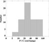 |
Fig. 3 Histogram of the parameter P/C for pixels with positive detection of the red bump. The scale of the x axis starts at a value of 5 and then every bin doubles the previous bin. |
4. Properties of the WR population in the CALIFA survey
4.1. The catalogue of WR-rich regions
Catalogue of galaxies showing WR features using the CALIFA survey data.
The selection procedure presented in Sect. 3 allows us to build a mask per galaxy pinpointing the location of those pixels satisfying criteria 1–5. We report the detection of regions with positive WR emission in a total of 25 galaxies. The main properties of these WR galaxies are listed in Table 1. Our catalogue of WR galaxies represents somewhat over 4% of the initial galaxy sample, which we recall is representative of the galaxy population in the Local Universe. As the CALIFA sample was not purposely selected to contain only galaxies with strong star formation episodes, a small percentage of galaxies with regions showing strong WR signatures is expected.
The WR host galaxies found are typically spirals and nearby blue dwarf galaxies with low inclination angles. Interestingly, 13 out of the 25 WR galaxies (52%) are related to galaxy interaction processes (galaxy pairs, signs of recent past interaction, or galaxies undergoing a merger). Also the majority of the WR galaxies analysed by López-Sánchez (2010) are also experiencing some kind of interaction.
It is surprising to find WR emission in an isolated Sa galaxy (NGC 1056), with lower disc star formation activity than late-type galaxies (Giuricin et al. 1994; Plauchu-Frayn et al. 2012), and in a dwarf elliptical (IC 0225; also detected in B08a, WR346). In fact, this dwarf galaxy is a peculiar object showing a blue core, which is very rare in these kinds of objects (Gu et al. 2006; Miller & Rudie 2008).
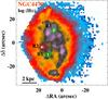 |
Fig. 4 Hα maps with logarithmic intensity scale of the galaxies with detected WR emission within the labelled regions enclosed by the green and red continuum contours. The pointed contours correspond with the associated Hα clump identified using HIIexplorer (Sánchez et al. 2012b), whenever the emission of the Hα clump is more extended than that of the WR region. A cross indicates the barycentre of the region. The scale corresponding to 2 kpc is drawn at the bottom left corner. North points up and east to the left. |
We identified a total of 44 WR-rich regions within the 25 galaxies listed in Table 1, individual WR regions per galaxy are numbered R1, R2, etc. Not all the WR regions are located in the centre of the galaxies, but rather they are distributed in the circumnuclear regions or found in external Hα clumps (e.g. NGC 5665). Figure 4 shows the Hα map of the galaxy NGC 4470, where three WR regions have been identified. Similar maps for the rest of the galaxies are shown in Fig. A.1. A third of the WR regions are located at projected distances further than half an effective radius, and the majority of these lies within one effective radius (see Fig. 5, left). The WR regions sometimes cover a fraction of the total area that is normally considered an H ii region (e.g. UGC 9663). In some cases, the WR regions are not apparently associated with an Hα clump or H ii -like region, but rather located within the Hα diffuse emission areas (e.g. R4 in NGC 5665). This suggests that some H ii regions are not resolved with our IFS data. For example, the H ii regions in the circumnuclear starburst in NGC 5953 (Casasola et al. 2010) are not resolved here but their WR emission has been detected. The main ionizing source of these regions usually is young, massive stars, as inferred from the diagnostic BPT diagram (Baldwin et al. 1981) shown in Fig. 5 (middle panel). Only the line ratios of one WR region is very close to the location of the AGN domain. This object is the nucleus of NGC 7469, a well-known Seyfert 1 galaxy with a circumnuclear starburst (Cutri et al. 1984; Heckman et al. 1986; Wilson et al. 1986), interacting with its companion IC 5283. The systematics of this effect could have produced a bias in searches of WR features with SDSS or other surveys of nearby galaxies (see e.g. Kehrig et al. 2013; Shirazi & Brinchmann 2012).
The main properties of the catalogue of the selected WR regions are listed in Table 2. Given that WR stars reside in H ii regions we tried, if possible, to associate the WR region with an Hα clump in order to define their radius. As expected, the Hα equivalent widths of these regions are close to or higher than 100 Å. The distribution of EW(Hα ) does not peak at the highest values, rather it peaks within the range 125–160 Å and then decreases (see Fig. 5, right). This is consistent with the fraction of star-forming galaxies that contain WR features as a function of EW(Hβ ) reported in B08a, where the curve reaches a maximum value and then turns over. This turnover is expected to happen when either EW(Hβ ) or EW(Hα ) (good indicators of the age of young populations) sample burst ages that are short relative to the starting time of the WR phase (after 2–3 Myr). Obviously, our measured equivalent widths actually represent lower limits to the real values because of the presence of underlying continuum of non-ionizing populations. That is the reason why, according to POPSTAR models, our peak represents ages of τ ~ 5.5 Myr, when the WR phase is practically about to end. Yet, the real shape of the curve or the distribution of equivalent widths (i.e. in this study) should be similar to the shapes reported. As already seen in the previous section with the spectra of the pixels, we detected the red bump in regions with higher EWs than average (150–300 Å). Taking into account that both bumps are originated in populations with similar age, this suggests that to better observe the red bump a lower contamination of the continuum by underlying non-ionizing populations seems to be necessary.
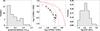 |
Fig. 5 Left: distribution of the WR region projected distance to the galaxy centre, normalized to the effective radius of the galaxy. Middle: [O iii]λ5007/Hβ vs. [N ii]λ6583/Hα diagnostic diagram (usually called the BPT diagram as described by Baldwin et al. 1981) for the selected regions. The solid and dashed lines indicate the Kewley et al. (2001) and Kauffmann et al. (2003) demarcation curves, respectively. These lines are usually used to distinguish between classical star-forming objects (below the dashed line) and AGN powered sources (above the solid line). Regions between both lines are considered to be of composite ionizing source. Right: distribution of the observed equivalent width of Hα in logarithmic units for the selected WR regions. |
Sample of regions found with positive detection of WR features.
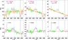 |
Fig. 6 Examples of the integrated observed spectra around the blue WR bump for three selected regions: R1 in NGC 1056 (left), R1 in IC 225 (middle), and R1 in NGC 3773 (right). The blue vertical line shows the location of the He iiλ4686 line. The significance level (εorig) is given on the top left corner. The red solid line shows a linear fit to the continuum. The green sections of the spectrum correspond to those spectral ranges used to compute the rms. The fitted continuum spectrum with STARLIGHT is overplotted in orange. Bottom: the corresponding continuum-subtracted spectra derived for each of the three selected regions. The value of ϵ is provided in each case. The flux is given in units of 10-16 erg s-1 cm-2 Å-1. |
For each WR region detected we added the spectra of all the corresponding spaxels to increase the signal-to-noise ratio (S/N) and perform a detailed analysis of its properties. We derived the star formation history (SFH) of the WR region using the STARLIGHT code to subtract the underlying stellar continuum. At this time we used a full set of several hundreds of stellar templates to perform a better modelling of their SFH.
We divided our WR region sample into two classes depending on the significance level of the observed integrated spectra, εorig. As shown in Fig. 6 the continuum is not only composed by noise but also by real absorption and emission stellar features. This fact is very notorious around 4500 Å, where the fitted continuum (solid orange line) follows well the observed continuum (solid green line) in the case of R1 in NGC 1056. Hence, the rms computed using this continuum is higher than that obtained using the subtracted fitted spectrum and hence it induces an increase of the significance level. However, when εorig is very low (e.g. region R1 in NGC 1056), ε is also higher because the WR feature is highly enhanced. We can also see that in this situation the continuum subtraction at the level of the emission feature is not very well achieved. Although slight deviations from a zero-valued horizontal line for the subtracted continuum is expected owing to fluctuations of the noise, in cases such as R1 in NGC 1056 the resulting subtracted continuum has a considerable slope. Therefore, the emission and shape of the WR feature depends extremely on the model subtraction when its detection level is close to the noise level in the observed spectrum. The higher the significance level in the observed spectrum, the lower the dependence on the model subtraction. For instance, for the spectrum of R1 in NGC 3773, ε is higher than εorig by a factor of 2, but this increase practically comes from the improvement of the continuum emission. The shape and area of the WR emission feature is very similar in the observed and subtracted spectrum.
Following this reasoning, we define as class-0 regions those with εorig< 5, and class-1 regions as those with higher significance level on the observed spectrum. Hence, with this subdivision we can distinguish between regions whose WR emission features highly depend on the continuum subtraction and those whose dependence is either not very significant or even negligible. Under this classification scheme, 14 regions are class-0 regions and the rest (30) are class-1 regions. Table 2 also lists this subdivision.
Finally, Table 2 indicates those regions with a positive detection of the red bump. In this case, the significance level of the detection is generally higher than 20, but only five WR regions with red bump have been found in our sample.
4.2. Multiple line fitting of the WR features
The exercise explained in the previous section showed that, in some cases, WR emission features emerge after stellar continuum subtraction in regions where there is a barely significant detection in the originally observed spectrum. In those cases, the emission line fluxes can be misleading since we are dealing with faint emission features at a continuum level where the uncertainties and systematics are not well understood. We therefore analysed WR features found only in class-1 regions, avoiding extremely model-dependent results, although class-0 regions still make a sample of promising candidates.
The blue bump is quite a complex emission structure formed from the blend of broad stellar lines of helium, nitrogen, and carbon: He iiλ4686, N vλλ4605, 4620, N iiiλλλ4628, 4634, 4640, and C iii /C ivλλ4650, 4658 (Conti & Massey 1989; Guseva et al. 2000; Crowther 2007). Furthermore, a number of nebular emission lines, such as the narrow He iiλ4686 emission line, [Fe iii] λλλ4658, 4665, 4703, [ArIV] λλ4711, 4740, He iλ4713, and [Ne iv] λ4713, are often superimposed on the broad features (Izotov & Thuan 1998; Guseva et al. 2000). This makes the disentangling of the individual fluxes rather challenging. These nebular emission lines within the bump should be properly removed and not included in the flux of the broad stellar lines.
In recent years, multiple Gaussian line-fitting procedures have been performed to fit this complex feature (e.g. B08a; López-Sánchez & Esteban 2010; MC14b). Following similar prescriptions used in those studies, we performed an automatic procedure to achieve a satisfactory fit in each case:
-
1.
The code fits a linear plus a Gaussian function to the broad He iiλ4686, to a broad feature centred at ~4645 Å, and to the two brightest nebular lines within this spectral range, [Fe iii] λ4658 and the narrow He iiλ4686. The chosen continuum windows are the spectral ranges 4500−4550 and 4750−4820 Å. The central wavelength of the Gaussian located at 4645 Å is set free within 15 Å. In that way, the code selects which blend is better observed: either the component centred around the nitrogen lines (~4634 Å) or the component centred around the carbon lines (~4650 Å). The width (σ) of the narrow (i.e. nebular) lines is fixed to that of Hβ , while the width of the broad components are set free with a maximum value of 22 Å (FWHM ~ 52 Å), which corresponds to a FWHM of about 3300 km s-1. This is appropriate taking into account the spectral resolution of the data (FWHM ~ 400 km s-1) and the typical upper limit adopted to the width of individual WR features (Smith & Willis 1982; Crowther 2007; B08a). If the code cannot successfully fit a nebular line (due to the absence of or low S/N), that component is discarded in the next step.
-
2.
If the width of the broad component centred at 4645 Å equals the maximum adopted value, a broad component around 4612 Å is included in the fit. If the added component is not successfully fitted, it is discarded.
-
3.
Next, the rms of the continuum is compared to the peak of the residuals. If this peak is higher than 4 × rms within the spectral range 4600−4750 Å, a new component is added. If the central wavelength of the new component is shorter than 4650 Å, it represents a broad emission line; in a few cases two distinct components are fitted, one centred at around 4634 Å and another at around 4650 Å. If the central wavelength of the new component is longer than 4650 Å, it is be considered a narrow line (i.e. a nebular line).
-
4.
Finally, the previous step is performed iteratively, adding a new component each time until the peak is lower than 4 × rms.
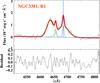 |
Fig. 7 Example of the multiple-line fit of WR features for the region found in NGC 3381. An almost horizontal blue line denotes the resulting continuum of the fit. The total fitted continuum plus emission lines on the blue bump is drawn with a thick red line. The nebular (blue) and broad stellar (green) components of the fit are also drawn. The vertical blue line indicates the position of the He iiλ4686 line. An auxiliary plot shows in black the residuals (in flux units) after modelling all the stellar and nebular features. |
In the case of R1 in NGC 7469, which is the nucleus of a Seyfert 1, we did not apply any continuum subtraction and just performed the fitting to the observed spectrum. Most Seyfert nuclei present a featureless ultraviolet and optical continuum following a power law, fν ∝ ν− α, that is attributed to a non-thermal source (Osterbrock 1978). Although within a diameter ≳2 kpc, the optical continuum is probably dominated by the stellar emission, and its modelling at the level of the weak emission of the WR features is quite poor because of the presence of a power-law component that is not included in the stellar libraries used in STARLIGHT . In any case, the significance level of the WR feature in the observed spectrum of this source is high enough (εorig = 8.9; see Table 2) so that a proper correction due to the continuum subtraction would probably not alter the emission shape of the WR feature significantly.
Regarding the red bump, basically two broad stellar lines form this broad emission feature, C ivλλ5801, 5812 (van der Hucht 2001; Ercolano et al. 2004). Given the broadness of these stellar lines, the auroral [N ii] λ5755 emission line is usually superposed on the red bump. Therefore, we fitted this narrow line together with a broad component centred at 5808 Å, setting the central wavelength of this broad component free within 20 Å. The fits are presented in Fig. A.3. We note that assuming a single broad component provided better results than fitting two close broad components. As we did for fitting the blue bump, an upper limit to the width of the broad component was needed. Hence, we adopted an upper limit of σ = 30 Å (FWHM ~ 70 Å). Changing this value by 5 Å induces a variation of ~10% in the integrated flux. We tried to include a fit to the C iiiλ5696 emission line, which is mainly originated in carbon WR subtypes, but given the noisy residual spectrum, even in the case of NGC 3773 (see Fig. A.3), no successful fit could be achieved with an uncertainty of less than 50%. Finally, this analysis does not include a fit to the nebular He iλ5876 emission line since, after the continuum subtraction, some residual emission up to ~5920 Å was still found. The intensities derived for the red bump are listed in Table 3, and are only a few percent of the Hβ emission.
5. Discussion
5.1. Nature and number of WR stars
Learning about the nature of the WR population from the measured lines that form the blue and red bumps is not an easy task. For instance, the broad He iiλ4686 and the blue bump emission are mainly linked to WN stars. Some emission from WC stars may also be expected in the blue WR bump (e.g. Schaerer & Vacca 1998), so all WR types contribute to this broad emission. The broad C ivλλ5801, 5812 emission feature essentially originates in WC stars (mainly in early types; WCE). However, given that this feature is harder to detect than the blue bump, its non-detection does not necessarily imply the absence of WC stars. Other lines that are directly linked with other WR subtypes (e.g. O viλλ3811, 3834, which are related to WO types) are not detected either. Finally, both WN and WC stars contribute to the emission of the broad N iiiλλλ4628, 4634, 4640 (WN) and C iii /C ivλλ4650, 4658 (WC) blends. Following MC14b, we consider these steps to identify the different subtypes of WRs that cause the WR bump emission for a given region and estimate their approximate number:
Fluxes derived from our fitting of the WR bumps, and derived WR numbers for the class-1 WR regions identified in this study.
-
Although He ii lines are also produced by O stars with ages τ ≲ 3 Myr (Schaerer & Vacca 1998; Massey et al. 2004; Brinchmann et al. 2008b), we assume that all the emission of the He iiλ4686 line comes from WRs.
-
The luminosity of WN late-type stars (WNL), which are the main contributors to the emission of the broad He iiλ4686 emission, is not constant and can vary within factors of a few. Given the reported metallicity dependence of this broad emission, we use the approach proposed by López-Sánchez & Esteban (2010) to estimate the luminosity of a single WNL, LWNL(He iiλ4686), as a function of metallicity,
 (2)with x = 12 + log(O/H).
 -
The N vλλ4605,4620 emission originates in early-type nitrogen stars (WNE). The mean luminosity of a single Large Magellanic Cloud WNE star is, with a dispersion of a factor of 2, about 1.6 × 1035 erg s-1 (Crowther & Hadfield 2006). These stars also contribute to the He iiλ4686 emission in about 8.4 × 1035 erg s-1.
-
Given that we do not observe the C iiiλ5696 line, which mainly originated in late-type WC stars, we assume that the red bump emission is mainly produced as a result of the presence of WCEs. We also use the approach proposed by López-Sánchez & Esteban (2010) this time to estimate the luminosity of a single WCE (LWCE,C ivλ5808), as a function of metallicity,
 (3)with x = 12 + log(O/H). These stars also
contribute to the emission of the broad He iiλ4686 line. The
estimation of the contribution of a single WCE to this emission feature is explained
in the following item.
(3)with x = 12 + log(O/H). These stars also
contribute to the emission of the broad He iiλ4686 line. The
estimation of the contribution of a single WCE to this emission feature is explained
in the following item. -
As mentioned before, the non-detection of the red bump does not guarantee that there are not WCs. MC14b estimated an upper limit to the number of WC stars in NGC 3310 to be in the range 5–20% of the number of WN stars. There, in general, EW(λ4650) <EW(λ4686). However, as can be seen in Table 3, in the current study EW(λ4650) is of the order of (or in some cases even higher than) EW(λ4686). This points towards a number of WC stars that are quite higher than just the 5%. Under these circumstances, we made a rough estimation of the number of WCEs even if no red bump was detected. To do that, a system of two equations with two unknowns has to be solved as follows:
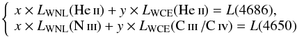 (4)where L(4686) and L(4650) refer to the
measured flux of the He iiλ4686 and λ4650 (including
N iiiλλλ4628-34-41 and C iii
/C ivλλ4650-58) broad features, respectively;
LWNL(He
ii ) and LWCE(He ii ) correspond
to the luminosity of a single WNL (from Eq. (2)) and a single WCE star in the λ4686 broad feature,
respectively; LWNL(N iii ) and
LWCE(C
iii / C iv ) indicate the luminosity of a
single WNL (3.8 ×
1035 erg s-1; Crowther &
Hadfield 2006) and a single WCE star in the λ4650 broad feature,
respectively; and the unkowns x and y are the number of
WNL and WCE stars. As reported in Crowther &
Hadfield (2006), the combined C iiiλ4650 +
H iiλ4686 flux of LMC WC4 stars averages around
49 × 1035
erg s-1. In
our study, 12% of this value is assigned to a contribution to the λ4686 feature,
whereas the remaining 88% is assumed for the contribution to the λ4650 emission. We
split it that way because several works support that the
He iiλ4686 emission in WC stars contributes on
average by 12% to the combined 4650/4686 blend (Schaerer & Vacca 1998; Smith et al.
1990), ranging from 8 to 30%. Finally, if the N vλλ4605, 4620 emission
is present in the spectra, the number of WNE stars is first obtained and then their
contribution to L(4686) is subtracted before solving the
equation system (Eq. (4)).
(4)where L(4686) and L(4650) refer to the
measured flux of the He iiλ4686 and λ4650 (including
N iiiλλλ4628-34-41 and C iii
/C ivλλ4650-58) broad features, respectively;
LWNL(He
ii ) and LWCE(He ii ) correspond
to the luminosity of a single WNL (from Eq. (2)) and a single WCE star in the λ4686 broad feature,
respectively; LWNL(N iii ) and
LWCE(C
iii / C iv ) indicate the luminosity of a
single WNL (3.8 ×
1035 erg s-1; Crowther &
Hadfield 2006) and a single WCE star in the λ4650 broad feature,
respectively; and the unkowns x and y are the number of
WNL and WCE stars. As reported in Crowther &
Hadfield (2006), the combined C iiiλ4650 +
H iiλ4686 flux of LMC WC4 stars averages around
49 × 1035
erg s-1. In
our study, 12% of this value is assigned to a contribution to the λ4686 feature,
whereas the remaining 88% is assumed for the contribution to the λ4650 emission. We
split it that way because several works support that the
He iiλ4686 emission in WC stars contributes on
average by 12% to the combined 4650/4686 blend (Schaerer & Vacca 1998; Smith et al.
1990), ranging from 8 to 30%. Finally, if the N vλλ4605, 4620 emission
is present in the spectra, the number of WNE stars is first obtained and then their
contribution to L(4686) is subtracted before solving the
equation system (Eq. (4)). 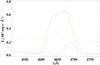
Fig. 8 Template of LMC WC (red), early WN (blue), and late WN (green) from Crowther & Hadfield (2006).
-
Finally, we must note that the fits performed on these features are not necessarily physical, since WC lines can be much broader than the upper limits adopted, as shown in Fig. 8 (as broad as almost the entire emission bump). Depending on the contribution of WC stars to the blue bump, the results might be misleading. We chose not to include another component to the fit that is much wider than the others with no clue on how to constrain it (in most cases the red bump is not detected). Instead, we tried to minimize this by fitting this feature directly, assigning different contributions of this emission to the C iiiλ4650 and H iiλ4686 fitted features, as mentioned in the previous item.
 (5)We consider the calibration proposed by Marino et al. (2013), which is valid for 12 + log(O/H) > 8.1 and has a dispersion somewhat lower than 0.2 dex. In any case, we compared the derived oxygen abundances with those obtained using the “counterpart” C-method introduced by Pilyugin et al. (2012), which is valid for all the metallicity ranges, and we obtained consistent values within 0.1 dex. The metallicities derived using the O3N2 calibration are listed in Table 3. The oxygen abundances range between 12 + log(O/H) = 8.2 and 8.6, where the typical value is about half of the solar value.
With this information we derived the number of WR stars for each subtype, when possible. The number of WNE, WNL, and WCE stars are compiled in the last columns of Table 3. We estimated the number of WNL and WCE stars by solving Eq. (4) in all cases, the number of WNE stars in just two cases (those showing a clear detection of the N vλλ4605,4620 blend), and the number of WCE stars using Eq. (3) in the five regions where the red WR bump is present in our spectra. In those cases in which the red bump is detected, we considered the number of WCE stars derived via the flux measurement of such a bump to compute their contribution to the broad He iiλ4686 emission. If we had not considered solving the system and instead if we had estimated the number of WNL stars using Eq. (2) directly, the resulting values would be higher by 10−20%.
The derived values span a wide range, from a few dozens in regions within the closest galaxies (NGC 4630 and UGC 6320) to more than 30 thousand in regions belonging to the most distant objects (NGC 6090 and NGC 7469). It is worth noting the detection of more than 30 thousand WRs in the nuclear region of a Seyfert 1 galaxy. It is not the first time that the coexistence of the AGN and a circumnuclear compact starburst located several hundreds of pc away has been reported (e.g. in Mrk 477, Heckman et al. 1997). In fact, the estimated number of WRs in that compact source amounts to about 30 thousand.
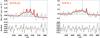 |
Fig. 9 R1 in IC 0776 as typical example showing the effects of the dilution for the spectrum of the WR region (left) and for the spectrum of the associated Hα clump (right). Lines and colours are the same as in Fig. 7. Some structure is lost and fewer nebular lines are fitted when the WR feature is diluted. It is also noticeable that the broad lines widen. |
We can compare the estimation of the number of WCE stars in those cases in which the red bump is detected, that is NWCE (RB) and NWCE (4650) in Table 3. Only in one case (NGC 3353) can we consider both values compatible within the uncertainties. A difference within a factor of two is encountered between both estimates in the remaining WR regions. This is not surprising given the uncertainties involved in these estimates, such as the possible systematics when using average luminosities that range enormously in each methodology; for instance, in Crowther & Hadfield 2006 luminosities of single WC4s in LMCs range from less than 2 to more than 4 × 1036 erg s-1. Finally, the number of WCEs that we obtain by solving the equation system (Eq. (4)) generally represents between 15 and 25% the number of WNLs4 as we expected, given that EW(λ 4650) ≳EW(λ 4686). We even find some unexpected cases (e.g. R1 in NGC 3994, R6 in NGC 5665, and R1 and R2 in UGC 00312) where EW(λ 4650) >2 × EW(λ 4686), and where the percentage is higher than 40%. Again, the systematics may play an important role in these estimates. All in all, we conclude that the estimates in the number of WCEs are probably correct within a factor of two.
5.2. Dilution of the WR features
One of the main biases when interpreting observational data is the limitation imposed by the spatial resolution. As mentioned before, WRs are usually very localized and sometimes the emission of the associated H ii region is significantly more extended, i.e. the spatial extent of WRs can be considerably smaller than that of the rest of the ionizing population (Kehrig et al. 2013). This is one of the main reasons why the emission of WRs easily dilutes in non-resolved studies. In this section, we discuss the effects of this dilution on the detectability and determination of the fluxes of the broad emission features when using the techniques described in this paper. Indeed, this directly affects the determination of the number of WR stars and constitutes a crucial step when interpreting the observed flux and when comparing them with stellar population models.
In several cases the spatial extent of the Hα clumps (i.e. H ii regions or aggregates) associated with our WR regions is larger than the area showing WR emission (see Fig. A.1). If we integrated the spectrum of these clumps, we would expect the WR bump to either disappear or dilute significantly. Then, if we performed the multiple fit of the WR emission features we would expect to obtain lower equivalent widths or detection significance. Several factors affect the final measured fluxes when the dilution effect is present:
-
Once the bump is diluted, its detection significance level decreases; and, if it is diluted too much it can actually disappear in the observed spectrum. As mentioned in Sect. 4.2, when εorig< 5, the shape of the WR feature is not very well constrained, since it is extremely model dependent on the continuum subtraction, which leads to unrealistic features. This happens, for instance, in R1 in IC 0225. When we integrate only the pixels showing WR features, εorig = 6.3, and when we integrate the whole Hα clump εorig = 4.2. In NGC 1056, the bump actually disappears in the observed spectrum (εorig = 2.6).
-
If the bump dilutes, barely resolved lines (i.e. weak nebular lines and weak broad components) dissolve, thus fewer and broader components are fitted. In order to properly interpret the measurement of the fluxes of the broad bump features, we have to correct for the nebular emission lines; specifically for the case of the broad He iiλ4686 line, we try to isolate it from the blend at 4640–4650 Å. This effect is illustrated in Fig. 9, for R1 in IC 0776.
-
In some cases, even if the same number of components are fitted, they become broader. If the lines are broader and the peak is similar then more flux is measured.
5.3. Comparison with stellar population models
5.3.1. Definition of the subsample
The Hα emission in H ii regions is typically more extended than the localized WR stellar emission in a given cluster, giving rise to the dilution effect discussed above, a fact that has to be taken into account when comparing spectroscopic observables with stellar population models. For instance, to make a proper comparison of the flux ratio of the blue bump to Hβ , we have to obtain the flux of Hβ from the whole H ii spectrum, as done for instance in B08a and discussed in Kehrig et al. (2013) for Mrk 178.
Aperture effects can also deceive the comparison with models in another way. Non-resolved Hα clumps with sizes of several hundreds of pc or larger can harbour several H ii regions. For instance, within an aperture of 1 kpc several regions in NGC 4630 are observed, but only the central region shows significant WR emission features. This can happen even at smaller apertures, such as in the giant H ii region Tol 89 in NGC 5398 (Sidoli et al. 2006). Within an aperture of about 300 pc there are at least two complexes (A and B) of massive (M> 105M⊙ ) clusters with ages within the range τ ~ 2−5 Myr, where the most massive and youngest (B) do not show signs of WR emission. Thus, if we compare the integrated WR and Hβ emission in this case, the interpretation of the properties of the population might be wrong. This gives us an idea that 100–200 pc can represent an appropriate aperture to perform these kinds of studies.
In this study, we performed this comparison for regions with a radius that is smaller than 400 pc (see Table 2) to have at least several regions at our disposal. Thus, in a few cases (NGC 3353, NGC 3381, NGC 5954) our results may still be somehow misleading provided that there is a cluster that is young enough so that WRs are still not present.
5.3.2. WR ratios and predictions from stellar population models
Empirical results, such as the ratio of WR to O stars, provide sensitive tests of evolutionary models, which involve complex processes (i.e. rotation, binarity, feedback, IMF, etc.) that remain not sufficiently constrained. This ratio can be roughly derived by first estimating the number of O stars using the Hβ luminosity. The Balmer emission in H ii regions is typically more extended than the localized WR stellar emission. Therefore, to properly compute the numer of O stars we have to use the Hβ luminosity of the whole Hα clump where the WR emission is detected. Then, assuming a contribution to the Hβ luminosity by an O7V star of LO7V = 4.76 × 1036 erg s-1, a first estimation of the number of such stars is obtained by NO7V = L(Hβ) /LO7V. Finally, the contribution of the WRs and other O subtypes to the ionizing flux is corrected as explained below:
-
Following Crowther & Hadfield (2006), the average numbers of ionizing photons of a WN and a WC star are assumed to be log
 and
and  , respectively.
 -
The total number of O stars (NO) can be derived from the number of O7V (NO7V) stars by correcting for other O stars subtypes, using the parameter η0 introduced by Vacca & Conti (1992) and Vacca (1994). This parameter depends on the initial mass function for massive stars and is a function of time because of their secular evolution (Schaerer & Vacca 1998). We made a rough estimation of the age of the population using the EW(Hβ ) measured on the H ii region spectra. This value was corrected by the emission of a non-stellar ionizing population, since the STARLIGHT code provides us with the SFH of the region (see Miralles-Caballero et al. 2014a). With the approximate knowledge of the age of the population, we estimated η0 using the SV98 models. The strongly non-linear temporal evolution of this parameter during some time intervals (see Fig. 21 in Schaerer & Vacca 1998) causes some asymmetries in the determination of its uncertainty. Table 4 lists the derived age, corrected EW(Hβ ) and estimated η0 for our subsample of regions.
 (6)where
  and
and  are the total and O7V number of ionizing photons, respectively. We adopted an average Lyman continuum flux per O7V star of log
  (Vacca & Conti 1992; Schaerer & Vacca 1998; Schaerer et al. 1999). The number of O stars and the WR to O ratio are reported in Table 4. The errors are generally large, making the high uncertainties involved when trying to derive these properties evident. In two cases (R1 in NGC 3353 and NGC 3381), the computed number of O stars is negative, which is a non-physical result. Nevertheless, given the large uncertainties involved in the determination of ηO and the number of each subtype of WR, we have been able to provide an upper limit within a confidence level of 90%. This allowed us to obtain a lower limit to the WR to O ratio. Given the large uncertainties involved, we ran a Monte Carlo simulation to obtain all the uncertainties. The median values in each simulation of NO and NWR/NO were the same to those obtained applying Eq. (6) directly to the derived average values of its elements, except for R1 in UGC 6320. Taking advantage of the Monte Carlo simulation, we realized that in this case a non-negligible percentage of estimates for NO were negative, which indicates that we were close to the noise level to obtain a physical result. Using the Bayessian approach we restricted the distribution considering only positive NO and then re-normalized this new distribution with only physical values. We thereby obtained a more representative value for NO by taking the median of the re-normalized distribution, which is reported in the table. The same accounts for NWR/NO for R1 in UGC 6320.
Derived properties of the WR population and WR number ratios.
Table 4 also provides the total estimated Lyman continuum flux and that emerging from WR stars. The contribution from the WR population is generally higher than the flux emerging from the other populations altogether. Even in those cases where the number of WR stars is almost negligible compared to that of O stars (around 4%, in NGC 5954 and in R2 in UGC 6320), the ionizing flux emerging from WR populations accounts for 30% of the total Lyman continuum budget.
We compared our observational data with the predictions of two different theoretical model sets: (i) POPSTAR (Mollá et al. 2009; Martín-Manjón et al. 2010), a self-consistent set of models including the chemical and spectro-photometric evolution, for spiral and irregular galaxies, where star formation and dust effects are important; and (ii) BPASS (Eldridge et al. 2008; Eldridge & Stanway 2009), which includes the binary evolution in modelling the stellar populations, which can extend the WR phase up to longer than 10 Myr. Both models use the photoionization code CLOUDY (Ferland et al. 1998) to predict the nebular emission.
The disagreement between models and data at moderate and low metallicities has been known for some time (e.g. Guseva et al. 2000; Crowther & Hadfield 2006; Pérez-Montero et al. 2010; López-Sánchez & Esteban 2010), especially when trying to explain the derived large WR to O ratios from observations. As discussed in Crowther (2007), the production of more WRs than currently favoured by the models can be achieved by including binarity in the evolutionary codes or when rotation is included in the stellar tracks. They have become promising sources for an increased WR population. In fact, several studies of samples of Galactic massive O stars support that binary interaction dominates the evolution of massive stars (e.g. Kobulnicky & Fryer 2007; Sana et al. 2012; Kiminki & Kobulnicky 2012). Eldridge et al. (2008) developed a synthesis population code, BPASS 5, where binarity is included. They found out that a third of the population evolves as single stars, while the remaining two-thirds correspond to interacting binaries. The inclusion of binaries led to a prolonged WR phase (up to τ ~ 15 Myr), which is consistent with earlier predictions by Van Bever & Vanbeveren (2003).
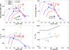 |
Fig. 10 Top: intensity ratio of the He ii 4686 Å broad line to Hβ (left) and the EW of the broad line (right) vs. EW (Hβ ), a good indicator of the age of young ionizing populations. The data are coloured depending on their metallicity. Tracks from POPSTAR (solid line; simple population) and BPASS (dashed line; binary population) are shown in different colours also depending on the metallicity. Open triangles indicate the values for 4.5 (small triangles) and 5.5 Myr (large triangles), respectively, on the POPSTAR tracks. Open circles indicate the values for 6 (small circles) and 12.5 Myr (large circles), respectively, on the BPASS tracks. The arrows labelled as FL = 2 and Fd = 2 illustrate how the tracks would move on the plot if half of the ionizing photons actually escape the ionized regions or are absorbed by dust grains within the H ii region. Bottom left: derived ratio of the number of WRs over the number of O stars vs. EW(Hβ ). Lower limits are provided for R1 in NGC 3381 and NGC 3773. Open diamonds show how the data would move in the plot if half of the photons escaped or were absorbed (the dotted lines connect each case); here, the upper limits disappear because with the increased Hβ flux , the derived number of O stars is not negative any more. The tracks from the BPASS models are completely horizontal because the only average values over the time of the WR phase are provided. Bottom right: ratio of the derived number of WC over WN stars vs. metallicity. Solid (dashed) line indicate the track for the POPSTAR (BPASS) model. |
As observed in Fig. 10 (top) simple stellar population models (POPSTAR ) are not able to reproduce, for the low-metallicity regions (Z ~ Z⊙/3), either the flux ratio I (broad He iiλ4686)/I(Hβ ) or the EW of the blue bump corrected by the continuum emission of the non-ionizing population. For the sake of completeness, we also show how the modelled tracks would move if half of the ionizing photons escape from the H ii regions (i.e. FL ≡ 2.0) or if they are absorbed by dust grains within the nebula (i.e. Fd ≡ 2.0). Thus, if we allow for some Lyman photon leakage or some absorption by dust grains within the nebula, the POPSTAR models could reproduce the flux ratio. In any case, however, for three regions only the binary models could explain the relatively high blue bump equivalent widths (Fig. 10, top right).
Reproducing the WR to O ratio, namely NWR/NO, is hard for the stellar population models, especially for the low-metallicity regions (Fig. 10, bottom-left). In addition, as mentioned in MC14b, this ratio can vary dramatically if we allow for some Lyman photon leakage, some absorption by dust grains within the nebula, or even a different IMF. This variation is not the same for all regions (as in the top panel), since if EW(Hβ ) increases, the age decreases and η0 (which is practically constant in some age bins and practically highly non-linear in others) may vary from almost nothing to dramatically, thus the variation of NWR/NO also ranges from almost nothing to a dramatic change. Those regions in which the ratio is higher than 0.2 cannot be reproduced at all with any kind of model if at least half of the ionizing photons are missing by either process (as might be the case for NGC 3381 R1 with NWR/NO> 1.75, where the value could decrease considerably if one takes into account photon leakage and/or the intrinsic absorption within the HII region, as shown in Fig. 10). Since the ratios in binary models are in general higher than those in simple models, the former are generally close to the observed ratios.
We were also able to compare the ratio of carbon to nitrogen WRs, namely NWC/NWN, with the predictions of models (Fig. 10, bottom-right), taking into account the high uncertainties involved especially when deriving NWC. While simple models predict ratios that are too high, our derived values are closer to the predictions made by binary models. Yet, discrepancies with factors of ~2 can be encountered. A similar agreement is generally found at moderate and low metallicities when the effects of rotation and binarity are included in the modelling (e.g. Neugent & Massey 2011; Neugent et al. 2012).
As a conclusion, we find that the observables can only be reproduced by simple star models in a few cases. In general, processes such as binarity, fast rotation, or even more complex processes (e.g. photon leakage, absorption by dust grains, and IMF variations) need to be included in the theoretical modelling of the stellar populations to better understand how massive stars evolve. This follows the recent line of discussion in observational studies of WR populations (e.g. Crowther 2007; B08a; López-Sánchez & Esteban 2010; Bibby & Crowther 2010, 2012; Kehrig et al. 2013).
5.4. WRs and the environment: the GRB-WR connection
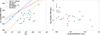 |
Fig. 11 Left: luminosity-metallicity (L−Z) relation of the galaxies in the CALIFA survey with detected WR stars. In grey those galaxies showing some signs of undergoing or recent interaction (M), and in blue those galaxies classified as isolated (I). L−Z relations for various galaxy samples from the literature are also drawn: UV-selected galaxies (solid orange; Contini et al. 2002), SDSS star-forming galaxies (solid blue; Tremonti et al. 2004), a large magnitude-limited sample (dotted pink; Lamareille et al.2004), irregular and spiral galaxies (dashed red; Kobulnicky et al. 1999), emission-line galaxies at z ~ 0.8 from the Deep Extragalactic Evolutionary Probe 2 survey (dot-dashed; Zahid et al. 2011) and star-forming BCGs (three dot-dashed green; Shi et al. (2005). The large error bars in the absolute magnitudes refer to the uncertainties in the galaxy distance moduli, taken from NED. Right: number density of WRs vs. their projected galactocentric distance. The colours of the regions denote if they belong to a merging (M) or an isolated (I) galaxy. Regions circled in red are those whose host galaxy does not follow the luminosity-metallicity relation and have a metallicity 12 + log (O/H) < 8.4 simultaneously. |
As mentioned in Sect. 4.1, 13 out of the 25 galaxies hosting WR regions show signs of interaction. Taking into account that young populations are also expected in normal spirals, irregulars, and dwarf blue galaxies, this fact suggests that the number of WRs is particularly high in galaxy interactions. This is not entirely surprising, since merging processes are known to enhance the star formation activity in the galaxies involved (e.g. Kennicutt et al. 1987; Barton Gillespie et al. 2003; Geller et al. 2006; Di Matteo et al. 2008; Rodríguez Zaurín et al. 2010; Barrera-Ballesteros et al. 2015). This is also in agreement with studies of supernova radial distributions that found SNe Ibc (those associated with more massive stars and GRBs) more centrally concentrated in disturbed/interacting galaxies (Habergham et al. 2012).
Very few studies have focused on the issue of connecting the environment of the galaxy, the presence of WRs, and the production of GRBs (e.g. Hammer et al. 2006; Han et al. 2010). MC14b investigated the environment of a single galaxy with strong presence WRs and tried to connect it with the properties of the hosts galaxies in Han et al. (2010), finding similarities in the integrated properties of GRB and WR hosts. A detailed study of the environment of local galaxies with similar properties to the GRB hosts is essential to better understand the physical properties of GRBs observed at moderate and high redshifts and the nature of their progenitors. The 25 galaxies with positive detection in this work allow us to dig deeper into this connection.
H10 performed a spectral analysis of eight LGRB hosts to study the environment in which such energetic events can take place. Since, according to the core-collapse model, WRs are considered the most favoured candidates to being the progenitors of LGRBs, the presence of WRs in their hosts provided evidence in favour of this theory. They identified some characteristics that support this connection. One of these characteristics is that these galaxies do not follow the luminosity- and mass-metallicity relations typically obeyed by irregular, spiral, and star-forming galaxies. The scenario of LGRBs occurring in host galaxies with lower metallicities than the general population is also supported by a few observational studies (e.g. Modjaz et al. 2011; Levesque et al. 2010a; Graham & Fruchter 2013). This under-abundance is naturally explained in galaxy mergers, since they induce radial gas mixing processes, such as inflows of external gas onto the central regions (e.g. Barnes & Hernquist 1996; Rupke et al. 2010).
We explored in Fig. 11 (left) whether our sample of host galaxies follow the luminosity-metallicity relation observed in the general population. We obtained the metallicity of the galaxies by integrating the whole spectrum within the CALIFA FoV and using the O3N2 calibration, as we did for the H ii regions. For metallicities higher than about 12 + log(O/H) = 8.4, the galaxies tend to follow the relation, although there are a couple of outliers. In contrast, galaxies with lower metallicities show a clear dichotomy: those with no clear signs of recent or current interaction processes (classified as isolated; I in Table 1) tend to follow the relation while those identified as merging (M in Table 1) are clearly outliers. Actually, even the most diverted object of the sample of isolated galaxies, UGC 10297, may present a disc truncation that could indicate a past minor merger (Comerón et al. 2012).
We have at least a subsample of about ten galaxies, most of which are undergoing an interaction, with similar characteristics to GRB hosts, namely moderate to low metallicity (Modjaz et al. 2011) and showing a significant offset in the luminosity-metallicity relation followed by the general galaxy population (Levesque et al. 2010b). But, are those hosts the ones that have larger number of WRs? Where are they located? Fig. 11 (right) shows a correlation between the number density of WRs (number of WRs/kpc2) and their projected distance to the centre of the galaxy. The Spearman correlation coefficient is very similar (ρ ~ −0.6) in regions from both the isolated and merging galaxy sample, which is somewhat stronger in the latter. While at distances shorter than about 0.3 reff several hundreds and even thousands of WR are observed per kpc2, in general an order of magnitude or less is observed at longer galactocentric distances.
The two regions with the highest number density are rather metal rich, and 2 regions out of 12 whose galaxies do not follow the luminosity-metallicity correlation have densities higher than 1000 WRs/kpc2. We could assume that in those 12 regions the probability for a GRB to occur is higher. Therefore, the existence of more WRs would not necessarily guarantee more GRB events and they would not necessarily be in the very central regions (where larger number of WR are found). In fact, there are some studies that do not associate the presence of GRBs with that of WRs, at least not in the exact location of the WRs but at spatial shifts of about hundreds of pc away (Hammer et al. 2006; Christensen et al. 2008; Levesque et al. 2011; Thöne et al. 2014). Yet, the presence of WRs is found in the host galaxies. In those studies, the location of the GRBs does not lie necessarily in the central regions of the galaxy either (e.g. in Thöne et al. 2014 it is found about 7–8 kpc away). Although we found galaxies with similar properties to the GRB hosts, more resolved studies of nearby GRB hosts are needed to better understand how these energetic phenomena occur and what their relation is with the WR population.
6. Conclusions
In this exploratory work, we have developed a technique to perform an automated search of Wolf-Rayet (WR) signatures through a pixel-by-pixel analysis of integral field spectroscopy (IFS) data of local galaxies. This procedure has been applied to a sample of 558 galaxies from the CALIFA survey plus the extended projects, spanning a wide range of physical properties. This represents the first systematic search of these peculiar populations in a large sample of galaxies observed with IFS, where we can have simultaneous spectral and spatial information. We present a catalogue of 44 regions with clear signatures of WR emission in the blue bump (five of these also show the red bump), in 25 star-forming galaxies presenting a variety of morphologies (and environments): irregulars, blue dwarfs, spirals, and interacting galaxies. We performed a detailed analysis of the main properties of these regions, drawing the following conclusions:
-
1.
We are able to detect WR emission in the spectrum of a pixel (with spatial scales spanning from 60 to about 600 pc) with equivalent widths (EW) of Hα that are typically higher than about 15 Å. The detection of the red bump implies less contamination by underlying non-ionizing populations, i.e. EW(Hα ) > 60 Å. For the candidate regions showing WR features, namely, WR regions, the distribution of EWs (ranging from 25 to 700 Å) peaks at 125–160 Å, decreasing at larger values (i.e. younger ages). The presence of a turnover in this distribution is consistent with the WR phase starting a few Myr after the population is born.
-
2.
While most of the regions are distributed within one effective radius, only a third of them are found at the centre of the galaxy, within ~1 kpc or less from the nucleus. While most WR regions are found in Hα clumps (i.e. H ii regions or aggregates), several seem to be associated with the diffuse Hα emission in the central regions of the galaxy, and they are not resolved and/or not distinguished because of the high Hα surface brightness in the centre of the galaxies.
-
3.
We performed a detailed fitting of the spectra of these regions considering the broad stellar and narrow nebular emission lines in the WR blue bump. Although large part of the emission is likely to be originated from late-type nitrogen WRs (WNL), direct positive detection from early-types (WNE) and carbon WRs (WC) has been obtained in two and five regions, respectively. Plausible evidence of a non-negligible percentage of early-type carbon WRs (WCEs) has been found in all regions. The WR regions host from dozens to more than 30 000 WRs, the most numerous regions are found in the two most distant galaxies. Actually, in one of the two (NGC 7469) direct evidence has been found for the existence of strong star formation with a large number of WRs and Seyfert activity within the central 2 kpc.
-
4.
There is a strong presence of WRs in galaxy interactions, irregulars, and blue dwarf galaxies, where strong star formation is observed. Galaxies showing signatures of recent past or undergoing merging processes have in general similar integrated properties to the hosts of gamma-ray burst events that also show an important presence of WR populations. However, the existence of a large number of WRs does not necessarily guarantee more GRB events or that they have to occur necessarily in the host very central regions. This is consistent with recent studies on GRB hosts.
-
5.
We discussed the effect of the dilution of the WR features when integrating the spectra at larger apertures than those where the feature is originally detected. These effects have to be taken into account when applying WR searching techniques that are currently widely used.
-
6.
We found clear evidence that the effects of binary stars and other processes (i.e. UV photon leakage, and absorption by UV photons within the H ii nebula) need to be taken into account in the stellar population modelling to better reproduce the observed fluxes of the WR stellar emission lines, equivalent widths, and the ratios of WR to O stars as well as between WR subtypes, especially at moderate to low metallicities. If binarity is important, the WR phase could last up to 10 Myr or so. Although very low metallicity regimes are not explored in this study, our result is consistent with previous studies that claim that simple star models fail dramatically to reproduce many of the observed properties of these stars in the Local Universe in low metallicity environments.
The spatial element with an independent spectrum is usually called spaxel in IFS; in this work we use pixel and spaxel indistinctly.
Should we assume the He iiλ4686 broad emission comes entirely from WNLs.
Acknowledgments
D.M.C., A.I.D., and F.F.R.O. would like to acknowledge financial support provided by the project AYA2010-21887-C04-03 (former Ministerio de Ciencia e Innovación, Spain) as well as the exchange programme “Study of Emission-Line Galaxies with Integral-Field Spectroscopy” (SELGIFS, FP7-PEOPLE-2013-IRSES-612701), funded by the EU through the IRSES scheme. A.M.I. acknowledges support from Agence Nationale de la Recherche through the STILISM project (ANR-12-BS05-0016-02). R.G.D. acknowledges support through the project AYA2014-57490-P. C.J.W. acknowledges support through the Marie Curie Career Integration Grant 303912. This research has made use of the NASA/IPAC Extragalactic Database (NED), which is operated by the Jet Propulsion Laboratory, California Institute of Technology, under contract with the National Aeronautics and Space Administration. Support for L.G. is provided by the Ministry of Economy, Development, and Tourism’s Millennium Science Initiative through grant IC120009, awarded to The Millennium Institute of Astrophysics, MAS. L.G. acknowledges support by CONICYT through FONDECYT grant 3140566.
References
- Abbott, J. B., Crowther, P. A., Drissen, L., et al. 2004, MNRAS, 350, 552 [NASA ADS] [CrossRef] [Google Scholar]
- Allen, D. A., Wright, A. E., & Goss, W. M. 1976, MNRAS, 177, 91 [NASA ADS] [Google Scholar]
- Alloin, D., Collin-Souffrin, S., Joly, M., & Vigroux, L. 1979, A&A, 78, 200 [Google Scholar]
- Baldwin, J. A., Phillips, M. M., & Terlevich, R. 1981, PASP, 93, 5 [NASA ADS] [CrossRef] [EDP Sciences] [Google Scholar]
- Barnes, J. E., & Hernquist, L. 1996, ApJ, 471, 115 [NASA ADS] [CrossRef] [Google Scholar]
- Barrera-Ballesteros, J. K., Sánchez, S. F., García-Lorenzo, B., et al. 2015, A&A, 579, A45 [NASA ADS] [CrossRef] [EDP Sciences] [Google Scholar]
- Barton Gillespie, E., Geller, M. J., & Kenyon, S. J. 2003, ApJ, 582, 668 [NASA ADS] [CrossRef] [Google Scholar]
- Bibby, J. L., & Crowther, P. A. 2010, MNRAS, 405, 2737 [NASA ADS] [Google Scholar]
- Bibby, J. L., & Crowther, P. A. 2012, MNRAS, 420, 3091 [NASA ADS] [CrossRef] [Google Scholar]
- Brinchmann, J., Kunth, D., & Durret, F. 2008a, A&A, 485, 657 [NASA ADS] [CrossRef] [EDP Sciences] [Google Scholar]
- Brinchmann, J., Pettini, M., & Charlot, S. 2008b, MNRAS, 385, 769 [NASA ADS] [CrossRef] [Google Scholar]
- Cairós, L. M., Caon, N., Zurita, C., et al. 2010, A&A, 520, A90 [NASA ADS] [CrossRef] [EDP Sciences] [Google Scholar]
- Cardelli, J. A., Clayton, G. C., & Mathis, J. S. 1989, ApJ, 345, 245 [NASA ADS] [CrossRef] [Google Scholar]
- Casasola, V., Hunt, L. K., Combes, F., et al. 2010, A&A, 510, A52 [NASA ADS] [CrossRef] [EDP Sciences] [Google Scholar]
- Castellanos, M., Díaz, A. I., & Terlevich, E. 2002, MNRAS, 337, 540 [NASA ADS] [CrossRef] [Google Scholar]
- Cerviño, M. 1998, Ph.D. Thesis, UMC, Spain [Google Scholar]
- Christensen, L., Vreeswijk, P. M., Sollerman, J., et al. 2008, A&A, 490, 45 [NASA ADS] [CrossRef] [EDP Sciences] [Google Scholar]
- Cid Fernandes, R., Gu, Q., Melnick, J., et al. 2004, MNRAS, 355, 273 [NASA ADS] [CrossRef] [Google Scholar]
- Cid Fernandes, R., Mateus, A., Sodré, L., Stasińska, G., & Gomes, J. M. 2005, MNRAS, 358, 363 [NASA ADS] [CrossRef] [Google Scholar]
- Cid Fernandes, R., Stasińska, G., Mateus, A., & Vale Asari, N. 2011, MNRAS, 413, 1687 [NASA ADS] [CrossRef] [Google Scholar]
- Comerón, S., Elmegreen, B. G., Salo, H., et al. 2012, ApJ, 759, 98 [NASA ADS] [CrossRef] [Google Scholar]
- Conti, P. S. 1991, ApJ, 377, 115 [NASA ADS] [CrossRef] [Google Scholar]
- Conti, P. S., & Massey, P. 1989, ApJ, 337, 251 [NASA ADS] [CrossRef] [Google Scholar]
- Contini, T., Treyer, M. A., Sullivan, M., & Ellis, R. S. 2002, MNRAS, 330, 75 [NASA ADS] [CrossRef] [Google Scholar]
- Crowther, P. A. 2007, ARA&A, 45, 177 [NASA ADS] [CrossRef] [Google Scholar]
- Crowther, P. A., & Hadfield, L. J. 2006, A&A, 449, 711 [NASA ADS] [CrossRef] [EDP Sciences] [Google Scholar]
- Crowther, P. A., Hadfield, L. J., Clark, J. S., Negueruela, I., & Vacca, W. D. 2006, MNRAS, 372, 1407 [NASA ADS] [CrossRef] [Google Scholar]
- Cutri, R. M., Rieke, G. H., Tokunaga, A. T., Willner, S. P., & Rudy, R. J. 1984, ApJ, 280, 521 [NASA ADS] [CrossRef] [Google Scholar]
- Dellenbusch, K. E., Gallagher, III, J. S., Knezek, P. M., & Noble, A. G. 2008, AJ, 135, 326 [NASA ADS] [CrossRef] [Google Scholar]
- Di Matteo, P., Bournaud, F., Martig, M., et al. 2008, A&A, 492, 31 [NASA ADS] [CrossRef] [EDP Sciences] [Google Scholar]
- Drissen, L., Moffat, A. F. J., & Shara, M. M. 1990, ApJ, 364, 496 [NASA ADS] [CrossRef] [Google Scholar]
- Drissen, L., Moffat, A. F. J., & Shara, M. M. 1993a, AJ, 105, 1400 [NASA ADS] [CrossRef] [Google Scholar]
- Drissen, L., Roy, J.-R., & Moffat, A. F. J. 1993b, AJ, 106, 1460 [NASA ADS] [CrossRef] [Google Scholar]
- Drissen, L., Crowther, P. A., Úbeda, L., & Martin, P. 2008, MNRAS, 389, 1033 [NASA ADS] [CrossRef] [Google Scholar]
- Eldridge, J. J., & Stanway, E. R. 2009, MNRAS, 400, 1019 [NASA ADS] [CrossRef] [Google Scholar]
- Eldridge, J. J., Izzard, R. G., & Tout, C. A. 2008, MNRAS, 384, 1109 [NASA ADS] [CrossRef] [Google Scholar]
- Ercolano, B., Wesson, R., Zhang, Y., et al. 2004, MNRAS, 354, 558 [NASA ADS] [CrossRef] [Google Scholar]
- Falcón-Barroso, J., Sánchez-Blázquez, P., Vazdekis, A., et al. 2011, A&A, 532, A95 [NASA ADS] [CrossRef] [EDP Sciences] [Google Scholar]
- Ferland, G. J., Korista, K. T., Verner, D. A., et al. 1998, PASP, 110, 761 [Google Scholar]
- Fruchter, A. S., Levan, A. J., Strolger, L., et al. 2006, Nature, 441, 463 [NASA ADS] [CrossRef] [PubMed] [Google Scholar]
- Galama, T. J., Vreeswijk, P. M., van Paradijs, J., et al. 1998, Nature, 395, 670 [NASA ADS] [CrossRef] [Google Scholar]
- Galbany, L., Stanishev, V., Mourão, A. M., et al. 2014, A&A, 572, A38 [NASA ADS] [CrossRef] [EDP Sciences] [Google Scholar]
- García-Benito, R., Díaz, A., Hägele, G. F., et al. 2010, MNRAS, 408, 2234 [NASA ADS] [CrossRef] [Google Scholar]
- García-Benito, R., Zibetti, S., Sánchez, S. F., et al. 2015, A&A, 576, A135 [NASA ADS] [CrossRef] [EDP Sciences] [Google Scholar]
- García-Lorenzo, B., Márquez, I., Barrera-Ballesteros, J. K., et al. 2015, A&A, 573, A59 [NASA ADS] [CrossRef] [EDP Sciences] [Google Scholar]
- Geller, M. J., Kenyon, S. J., Barton, E. J., Jarrett, T. H., & Kewley, L. J. 2006, AJ, 132, 2243 [NASA ADS] [CrossRef] [Google Scholar]
- Giuricin, G., Monaco, P., Mardirossian, F., & Mezzetti, M. 1994, ApJ, 425, 450 [NASA ADS] [CrossRef] [Google Scholar]
- González Delgado, R. M., & Pérez, E. 1997, ApJS, 108, 199 [NASA ADS] [CrossRef] [Google Scholar]
- Gonzalez-Delgado, R. M., Perez, E., Tenorio-Tagle, G., et al. 1994, ApJ, 437, 239 [NASA ADS] [CrossRef] [Google Scholar]
- Gonzalez-Delgado, R. M., Perez, E., Diaz, A. I., et al. 1995, ApJ, 439, 604 [NASA ADS] [CrossRef] [Google Scholar]
- González Delgado, R. M., Cerviño, M., et al. 2005, MNRAS, 357, 945 [NASA ADS] [CrossRef] [Google Scholar]
- Graham, J. F., & Fruchter, A. S. 2013, ApJ, 774, 119 [CrossRef] [Google Scholar]
- Gu, Q., Zhao, Y., Shi, L., Peng, Z., & Luo, X. 2006, AJ, 131, 806 [NASA ADS] [CrossRef] [Google Scholar]
- Guseva, N. G., Izotov, Y. I., & Thuan, T. X. 2000, ApJ, 531, 776 [NASA ADS] [CrossRef] [Google Scholar]
- Habergham, S. M., James, P. A., & Anderson, J. P. 2012, MNRAS, 424, 2841 [NASA ADS] [CrossRef] [Google Scholar]
- Hadfield, L. J., & Crowther, P. A. 2006, MNRAS, 368, 1822 [NASA ADS] [CrossRef] [Google Scholar]
- Hadfield, L. J., & Crowther, P. A. 2007, MNRAS, 381, 418 [NASA ADS] [CrossRef] [Google Scholar]
- Hadfield, L. J., Crowther, P. A., Schild, H., & Schmutz, W. 2005, A&A, 439, 265 [NASA ADS] [CrossRef] [EDP Sciences] [Google Scholar]
- Hainich, R., Rühling, U., Todt, H., et al. 2014, A&A, 565, A27 [NASA ADS] [CrossRef] [EDP Sciences] [Google Scholar]
- Hammer, F., Flores, H., Schaerer, D., et al. 2006, A&A, 454, 103 [NASA ADS] [CrossRef] [EDP Sciences] [Google Scholar]
- Han, X. H., Hammer, F., Liang, Y. C., et al. 2010, A&A, 514, A24 [NASA ADS] [CrossRef] [EDP Sciences] [Google Scholar]
- Heckman, T. M., Beckwith, S., Blitz, L., Skrutskie, M., & Wilson, A. S. 1986, ApJ, 305, 157 [NASA ADS] [CrossRef] [Google Scholar]
- Heckman, T. M., González-Delgado, R., Leitherer, C., et al. 1997, ApJ, 482, 114 [NASA ADS] [CrossRef] [Google Scholar]
- Hjorth, J., Sollerman, J., Møller, P., et al. 2003, Nature, 423, 847 [NASA ADS] [CrossRef] [PubMed] [Google Scholar]
- Ho, L. C., Filippenko, A. V., & Sargent, W. L. 1995, ApJS, 98, 477 [NASA ADS] [CrossRef] [Google Scholar]
- Hunt, L. K., & Hirashita, H. 2009, A&A, 507, 1327 [NASA ADS] [CrossRef] [EDP Sciences] [Google Scholar]
- Husemann, B., Jahnke, K., Sánchez, S. F., et al. 2013, A&A, 549, A87 [NASA ADS] [CrossRef] [EDP Sciences] [Google Scholar]
- Izotov, Y. I., & Thuan, T. X. 1998, ApJ, 500, 188 [NASA ADS] [CrossRef] [Google Scholar]
- Izotov, Y. I., Thuan, T. X., & Lipovetsky, V. A. 1997, ApJS, 108, 1 [NASA ADS] [CrossRef] [Google Scholar]
- James, B. L., Tsamis, Y. G., Barlow, M. J., et al. 2009, MNRAS, 398, 2 [NASA ADS] [CrossRef] [Google Scholar]
- Karthick, M. C., López-Sánchez, Á. R., Sahu, D. K., Sanwal, B. B., & Bisht, S. 2014, MNRAS, 439, 157 [NASA ADS] [CrossRef] [Google Scholar]
- Kauffmann, G., Heckman, T. M., Tremonti, C., et al. 2003, MNRAS, 346, 1055 [Google Scholar]
- Kehrig, C., Vílchez, J. M., Sánchez, S. F., et al. 2008, A&A, 477, 813 [NASA ADS] [CrossRef] [EDP Sciences] [Google Scholar]
- Kehrig, C., Pérez-Montero, E., Vílchez, J. M., et al. 2013, MNRAS, 432, 2731 [NASA ADS] [CrossRef] [Google Scholar]
- Kelly, P. L., Kirshner, R. P., & Pahre, M. 2008, ApJ, 687, 1201 [NASA ADS] [CrossRef] [Google Scholar]
- Kelz, A., Verheijen, M. A. W., Roth, M. M., et al. 2006, PASP, 118, 129 [NASA ADS] [CrossRef] [Google Scholar]
- Kennicutt, Jr., R. C. 1984, ApJ, 287, 116 [NASA ADS] [CrossRef] [Google Scholar]
- Kennicutt, Jr., R. C., Roettiger, K. A., Keel, W. C., van der Hulst, J. M., & Hummel, E. 1987, AJ, 93, 1011 [NASA ADS] [CrossRef] [Google Scholar]
- Kewley, L. J., Dopita, M. A., Sutherland, R. S., Heisler, C. A., & Trevena, J. 2001, ApJ, 556, 121 [Google Scholar]
- Kiminki, D. C., & Kobulnicky, H. A. 2012, ApJ, 751, 4 [NASA ADS] [CrossRef] [Google Scholar]
- Kobulnicky, H. A., & Fryer, C. L. 2007, ApJ, 670, 747 [NASA ADS] [CrossRef] [Google Scholar]
- Kobulnicky, H. A., & Zaritsky, D. 1999, ApJ, 511, 118 [NASA ADS] [CrossRef] [Google Scholar]
- Kudritzki, R. P. 2002, ApJ, 577, 389 [NASA ADS] [CrossRef] [Google Scholar]
- Kunth, D., & Joubert, M. 1985, A&A, 142, 411 [NASA ADS] [Google Scholar]
- Kunth, D., & Sargent, W. L. W. 1981, A&A, 101, L5 [NASA ADS] [Google Scholar]
- Kunth, D., & Sargent, W. L. W. 1983, ApJ, 273, 81 [NASA ADS] [CrossRef] [Google Scholar]
- Lamareille, F., Mouhcine, M., Contini, T., Lewis, I., & Maddox, S. 2004, MNRAS, 350, 396 [NASA ADS] [CrossRef] [Google Scholar]
- Leloudas, G., Sollerman, J., Levan, A. J., et al. 2010, A&A, 518, A29 [NASA ADS] [CrossRef] [EDP Sciences] [Google Scholar]
- Levesque, E. M., Berger, E., Kewley, L. J., & Bagley, M. M. 2010a, AJ, 139, 694 [NASA ADS] [CrossRef] [Google Scholar]
- Levesque, E. M., Kewley, L. J., Berger, E., & Zahid, H. J. 2010b, AJ, 140, 1557 [NASA ADS] [CrossRef] [Google Scholar]
- Levesque, E. M., Berger, E., Soderberg, A. M., & Chornock, R. 2011, ApJ, 739, 23 [NASA ADS] [CrossRef] [Google Scholar]
- Lopez, L. A., Krumholz, M. R., Bolatto, A. D., Prochaska, J. X., & Ramirez-Ruiz, E. 2011, ApJ, 731, 91 [NASA ADS] [CrossRef] [Google Scholar]
- López-Sánchez, Á. R. 2010, A&A, 521, A63 [NASA ADS] [CrossRef] [EDP Sciences] [Google Scholar]
- López-Sánchez, Á. R., & Esteban, C. 2010, A&A, 516, A104 [NASA ADS] [CrossRef] [EDP Sciences] [Google Scholar]
- López-Sánchez, Á. R., Mesa-Delgado, A., López-Martín, L., & Esteban, C. 2011, MNRAS, 411, 2076 [NASA ADS] [CrossRef] [Google Scholar]
- López-Sánchez, Á. R., Dopita, M. A., Kewley, L. J., et al. 2012, MNRAS, 426, 2630 [NASA ADS] [CrossRef] [Google Scholar]
- Marino, R. A., Rosales-Ortega, F. F., Sánchez, S. F., et al. 2013, A&A, 559, A114 [NASA ADS] [CrossRef] [EDP Sciences] [Google Scholar]
- Martín-Manjón, M. L., García-Vargas, M. L., Mollá, M., & Díaz, A. I. 2010, MNRAS, 403, 2012 [NASA ADS] [CrossRef] [Google Scholar]
- Massey, P. 2003, ARA&A, 41, 15 [NASA ADS] [CrossRef] [Google Scholar]
- Massey, P., & Hunter, D. A. 1998, ApJ, 493, 180 [NASA ADS] [CrossRef] [Google Scholar]
- Massey, P., Bresolin, F., Kudritzki, R. P., Puls, J., & Pauldrach, A. W. A. 2004, ApJ, 608, 1001 [Google Scholar]
- Meynet, G. 1995, A&A, 298, 767 [NASA ADS] [Google Scholar]
- Meynet, G., & Maeder, A. 2005, A&A, 429, 581 [Google Scholar]
- Miller, B. W., & Rudie, G. 2008, in IAU Symp. 245, eds. M. Bureau, E. Athanassoula, & B. Barbuy, 311 [Google Scholar]
- Miralles-Caballero, D., Colina, L., Arribas, S., & Duc, P.-A. 2011, AJ, 142, 79 [NASA ADS] [CrossRef] [Google Scholar]
- Miralles-Caballero, D., Díaz, A. I., Rosales-Ortega, F. F., Pérez-Montero, E., & Sánchez, S. F. 2014a, MNRAS, 440, 2265 [NASA ADS] [CrossRef] [Google Scholar]
- Miralles-Caballero, D., Rosales-Ortega, F. F., Díaz, A. I., et al. 2014b, MNRAS, 445, 3803 [NASA ADS] [CrossRef] [Google Scholar]
- Modjaz, M., Stanek, K. Z., Garnavich, P. M., et al. 2006, ApJ, 645, L21 [NASA ADS] [CrossRef] [Google Scholar]
- Modjaz, M., Kewley, L., Bloom, J. S., et al. 2011, ApJ, 731, L4 [NASA ADS] [CrossRef] [Google Scholar]
- Mollá, M., García-Vargas, M. L., & Bressan, A. 2009, MNRAS, 398, 451 [NASA ADS] [CrossRef] [Google Scholar]
- Monreal-Ibero, A., Vílchez, J. M., Walsh, J. R., & Muñoz-Tuñón, C. 2010, A&A, 517, A27 [NASA ADS] [CrossRef] [EDP Sciences] [Google Scholar]
- Monreal-Ibero, A., Walsh, J. R., & Vílchez, J. M. 2012, A&A, 544, A60 [NASA ADS] [CrossRef] [EDP Sciences] [Google Scholar]
- Monreal-Ibero, A., Walsh, J. R., Westmoquette, M. S., & Vílchez, J. M. 2013, A&A, 553, A57 [NASA ADS] [CrossRef] [EDP Sciences] [Google Scholar]
- Neugent, K. F., & Massey, P. 2011, ApJ, 733, 123 [NASA ADS] [CrossRef] [Google Scholar]
- Neugent, K. F., Massey, P., & Georgy, C. 2012, ApJ, 759, 11 [NASA ADS] [CrossRef] [Google Scholar]
- Osterbrock, D. E. 1978, Proc. Nat. Acad. Sci., 75, 540 [Google Scholar]
- Osterbrock, D. E. 1989, Astrophysics of Gaseous Nebulae and Active Galactic Nuclei (Sausalito, California: University Science Books) [Google Scholar]
- Osterbrock, D. E., & Cohen, R. D. 1982, ApJ, 261, 64 [NASA ADS] [CrossRef] [Google Scholar]
- Pérez-Montero, E., & Díaz, Á. I. 2007, MNRAS, 377, 1195 [NASA ADS] [CrossRef] [Google Scholar]
- Pérez-Montero, E., García-Benito, R., Hägele, G. F., & Díaz, Á. I. 2010, MNRAS, 404, 2037 [NASA ADS] [Google Scholar]
- Perez-Montero, E., Kehrig, C., Brinchmann, J., et al. 2013, Adv. Astron., 837392 [Google Scholar]
- Pilyugin, L. S., Grebel, E. K., & Mattsson, L. 2012, MNRAS, 424, 2316 [NASA ADS] [CrossRef] [Google Scholar]
- Plauchu-Frayn, I., Del Olmo, A., Coziol, R., & Torres-Papaqui, J. P. 2012, A&A, 546, A48 [NASA ADS] [CrossRef] [EDP Sciences] [Google Scholar]
- Rodríguez Zaurín, J., Tadhunter, C. N., & González Delgado, R. M. 2010, MNRAS, 403, 1317 [NASA ADS] [CrossRef] [Google Scholar]
- Rosales-Ortega, F. F., Kennicutt, R. C., Sánchez, S. F., et al. 2010, MNRAS, 405, 735 [NASA ADS] [Google Scholar]
- Roth, M. M., Kelz, A., Fechner, T., et al. 2005, PASP, 117, 620 [NASA ADS] [CrossRef] [Google Scholar]
- Rupke, D. S. N., Kewley, L. J., & Barnes, J. E. 2010, ApJ, 710, L156 [NASA ADS] [CrossRef] [Google Scholar]
- Sana, H., de Mink, S. E., de Koter, A., et al. 2012, Science, 337, 444 [Google Scholar]
- Sánchez, S. F., Kennicutt, R. C., Gil de Paz, A., et al. 2012a, A&A, 538, A8 [NASA ADS] [CrossRef] [EDP Sciences] [Google Scholar]
- Sánchez, S. F., Rosales-Ortega, F. F., Marino, R. A., et al. 2012b, A&A, 546, A2 [NASA ADS] [CrossRef] [EDP Sciences] [Google Scholar]
- Sánchez, S. F., Rosales-Ortega, F. F., Iglesias-Páramo, J., et al. 2014, A&A, 563, A49 [NASA ADS] [CrossRef] [EDP Sciences] [Google Scholar]
- Sánchez-Portal, M., Díaz, Á. I., Terlevich, R., et al. 2000, MNRAS, 312, 2 [Google Scholar]
- Sander, A., Todt, H., Hainich, R., & Hamann, W.-R. 2014, A&A, 563, A89 [NASA ADS] [CrossRef] [EDP Sciences] [Google Scholar]
- Sargent, W. L. W., & Filippenko, A. V. 1991, AJ, 102, 107 [NASA ADS] [CrossRef] [Google Scholar]
- Schaerer, D., & Vacca, W. D. 1998, ApJ, 497, 618 [NASA ADS] [CrossRef] [Google Scholar]
- Schaerer, D., Contini, T., & Kunth, D. 1999, A&A, 341, 399 [NASA ADS] [Google Scholar]
- Schild, H., Crowther, P. A., Abbott, J. B., & Schmutz, W. 2003, A&A, 397, 859 [NASA ADS] [CrossRef] [EDP Sciences] [Google Scholar]
- Shara, M. M., Bibby, J. L., Zurek, D., et al. 2013, AJ, 146, 162 [NASA ADS] [CrossRef] [Google Scholar]
- Shi, F., Kong, X., Li, C., & Cheng, F. Z. 2005, A&A, 437, 849 [NASA ADS] [CrossRef] [EDP Sciences] [Google Scholar]
- Shirazi, M., & Brinchmann, J. 2012, MNRAS, 421, 1043 [NASA ADS] [CrossRef] [Google Scholar]
- Sidoli, F., Smith, L. J., & Crowther, P. A. 2006, MNRAS, 370, 799 [NASA ADS] [CrossRef] [Google Scholar]
- Smith, L. J., & Willis, A. J. 1982, MNRAS, 201, 451 [NASA ADS] [Google Scholar]
- Smith, L. F., Shara, M. M., & Moffat, A. F. J. 1990, ApJ, 348, 471 [NASA ADS] [CrossRef] [Google Scholar]
- Stanek, K. Z., Matheson, T., Garnavich, P. M., et al. 2003, ApJ, 591, L17 [NASA ADS] [CrossRef] [Google Scholar]
- Thöne, C. C., Christensen, L., Prochaska, J. X., et al. 2014, MNRAS, 441, 2034 [NASA ADS] [CrossRef] [Google Scholar]
- Tremonti, C. A., Heckman, T. M., Kauffmann, G., et al. 2004, ApJ, 613, 898 [NASA ADS] [CrossRef] [Google Scholar]
- Tresse, L., Maddox, S., Loveday, J., & Singleton, C. 1999, MNRAS, 310, 262 [NASA ADS] [CrossRef] [Google Scholar]
- Úbeda, L., & Drissen, L. 2009, MNRAS, 394, 1847 [NASA ADS] [CrossRef] [Google Scholar]
- Vacca, W. D. 1994, ApJ, 421, 140 [NASA ADS] [CrossRef] [Google Scholar]
- Vacca, W. D., & Conti, P. S. 1992, ApJ, 401, 543 [NASA ADS] [CrossRef] [Google Scholar]
- Van Bever, J., & Vanbeveren, D. 2003, A&A, 400, 63 [NASA ADS] [CrossRef] [EDP Sciences] [Google Scholar]
- van Bever, J., & Vanbeveren, D. 2007, in Massive Stars in Interactive Binaries, eds. N. St.-Louis & A. F. J. Moffat, ASP Conf. Ser., 367, 579 [Google Scholar]
- van der Hucht, K. A. 2001, VizieR Online Data Catalog, III/215 [Google Scholar]
- Vazdekis, A., Sánchez-Blázquez, P., Falcón-Barroso, J., et al. 2010, MNRAS, 404, 1639 [NASA ADS] [Google Scholar]
- Walcher, C. J., Wisotzki, L., Bekeraité, S., et al. 2014, A&A, 569, A1 [NASA ADS] [CrossRef] [EDP Sciences] [Google Scholar]
- Westmoquette, M. S., James, B., Monreal-Ibero, A., & Walsh, J. R. 2013, A&A, 550, A88 [NASA ADS] [CrossRef] [EDP Sciences] [Google Scholar]
- Wilson, A. S., Baldwin, J. A., Sun, S.-D., & Wright, A. E. 1986, ApJ, 310, 121 [NASA ADS] [CrossRef] [Google Scholar]
- Woosley, S. E., & Heger, A. 2006, ApJ, 637, 914 [NASA ADS] [CrossRef] [Google Scholar]
- Youngblood, A. J., & Hunter, D. A. 1999, ApJ, 519, 55 [NASA ADS] [CrossRef] [Google Scholar]
- Zahid, H. J., Kewley, L. J., & Bresolin, F. 2011, ApJ, 730, 137 [NASA ADS] [CrossRef] [Google Scholar]
Appendix A: Additional figures
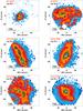 |
Fig. A.1 Hα maps with logarithmic intensity scale of the galaxies with detected WR emission within the labelled regions enclosed by green and red continuum contours. The pointed contours correspond to the associated Hα clump identified using HIIexplorer, whenever the emission of the Hα clump is more extended than that of the WR region. A cross indicates the barycentre of the region. The scale corresponding to 2 kpc is drawn at the bottom left corner. North points up and east to the left. |
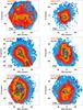 |
Fig. A.1 continued. |
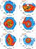 |
Fig. A.1 continued. |
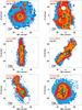 |
Fig. A.1 continued. |
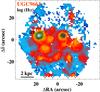 |
Fig. A.1 continued. |
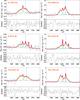 |
Fig. A.2 Multiple-line fit of WR features within the blue bump. An almost horizontal blue line denotes the resulting continuum of the fit. The total fitted continuum plus emission lines to the blue bump is drawn with a thick red line. The nebular (blue) and broad stellar (green) components of the fit are also drawn. The vertical blue line indicates the position of the He ii 4686 Å line. In each case, an auxiliary plot shows in black the residuals (in flux units) after modelling all the stellar and nebular features. For the case of NGC 7469, the fitting has been carried out on the observed spectrum, as explained in the text. |
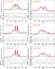 |
Fig. A.2 continued. |
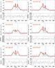 |
Fig. A.2 continued. |
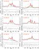 |
Fig. A.2 continued. |
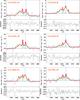 |
Fig. A.2 continued. |
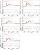 |
Fig. A.3 Multiple-line fit of WR features within the red bump. In each figure the residual spectrum is shown in black. This corresponds to the emission gaseous and stellar line spectrum minus the modelled feature in flux units. An almost horizontal blue line denotes the resulting continuum of the fit. The total fitted continuum plus emission lines to the blue bump is drawn with a thick red line. The fit to the auroral [N ii] 5755 Å line (blue) and broad stellar C iv 5808 Å feature (green) components of the fit are also drawn. The vertical red line indicates the position of the C iv 5808 Å feature. |
All Tables
Fluxes derived from our fitting of the WR bumps, and derived WR numbers for the class-1 WR regions identified in this study.
All Figures
|
Fig. 1 Top: examples of continuum-subtracted spectra for a given pixel in NGC 3991 and NGC 3381 around the blue WR bump spectral range. The blue vertical line shows the location of the He iiλ4686 emission line. The spatial coordinates of the pixels (x and y) and the P/C, ϵ, and PWR parameters defined in the text are given on the left-top corner of each panel. A red continuous line indicates a linear fit to the continuum (which ideally should be an horizontal line at y = 0). The green sections of the spectrum correspond to those spectral ranges used to compute the rms. Bottom: examples of continuum-subtracted spectra for a given pixel in NGC 3773 around the red WR bump spectral range. The red vertical line indicates the location of the C ivλ5808 emission line. The coordinates of the pixels and their associated parameters are also given on the left-top corner. In both the blue and the red WR bump cases one spectrum at the limit of the detection level (left) and another with a very good detection level (right) are shown. The flux density is given in units of 10-16 erg s-1 cm-2 Å-1. |
| In the text | |
|
Fig. 2 Left: density plot (grey scale) of P/C vs. ε parameters for all the pixels in the sample for which P/C > 0.85. Contours that contain 68% (1σ), 95% (2σ) and 99% (3σ) of the points are overplotted. Red dots correspond to the values of the pre-selected regions, i.e. before imposing the grouping of at least 9 pixels. Middle: same as before, but this time the overplotted green dots correspond to selected regions, also obeying the grouping criterion. The orange vertical line indicates the cut used for ε (4), while the horizontal line denotes P/C ~ 2.1 parameter, having practically all the selected pixels a higher value than this limit. Right: histogram of ε for pixels with P/C > 0.85 (black), pre-selected pixels (red), selected pixels (green), and for those pre-selected pixels not satisfying the grouping criterion (dotted black). The curve resulting from a Gaussian fit of the black histogram is overplotted in blue. |
| In the text | |
|
Fig. 3 Histogram of the parameter P/C for pixels with positive detection of the red bump. The scale of the x axis starts at a value of 5 and then every bin doubles the previous bin. |
| In the text | |
|
Fig. 4 Hα maps with logarithmic intensity scale of the galaxies with detected WR emission within the labelled regions enclosed by the green and red continuum contours. The pointed contours correspond with the associated Hα clump identified using HIIexplorer (Sánchez et al. 2012b), whenever the emission of the Hα clump is more extended than that of the WR region. A cross indicates the barycentre of the region. The scale corresponding to 2 kpc is drawn at the bottom left corner. North points up and east to the left. |
| In the text | |
|
Fig. 5 Left: distribution of the WR region projected distance to the galaxy centre, normalized to the effective radius of the galaxy. Middle: [O iii]λ5007/Hβ vs. [N ii]λ6583/Hα diagnostic diagram (usually called the BPT diagram as described by Baldwin et al. 1981) for the selected regions. The solid and dashed lines indicate the Kewley et al. (2001) and Kauffmann et al. (2003) demarcation curves, respectively. These lines are usually used to distinguish between classical star-forming objects (below the dashed line) and AGN powered sources (above the solid line). Regions between both lines are considered to be of composite ionizing source. Right: distribution of the observed equivalent width of Hα in logarithmic units for the selected WR regions. |
| In the text | |
|
Fig. 6 Examples of the integrated observed spectra around the blue WR bump for three selected regions: R1 in NGC 1056 (left), R1 in IC 225 (middle), and R1 in NGC 3773 (right). The blue vertical line shows the location of the He iiλ4686 line. The significance level (εorig) is given on the top left corner. The red solid line shows a linear fit to the continuum. The green sections of the spectrum correspond to those spectral ranges used to compute the rms. The fitted continuum spectrum with STARLIGHT is overplotted in orange. Bottom: the corresponding continuum-subtracted spectra derived for each of the three selected regions. The value of ϵ is provided in each case. The flux is given in units of 10-16 erg s-1 cm-2 Å-1. |
| In the text | |
|
Fig. 7 Example of the multiple-line fit of WR features for the region found in NGC 3381. An almost horizontal blue line denotes the resulting continuum of the fit. The total fitted continuum plus emission lines on the blue bump is drawn with a thick red line. The nebular (blue) and broad stellar (green) components of the fit are also drawn. The vertical blue line indicates the position of the He iiλ4686 line. An auxiliary plot shows in black the residuals (in flux units) after modelling all the stellar and nebular features. |
| In the text | |
|
Fig. 8 Template of LMC WC (red), early WN (blue), and late WN (green) from Crowther & Hadfield (2006). |
| In the text | |
|
Fig. 9 R1 in IC 0776 as typical example showing the effects of the dilution for the spectrum of the WR region (left) and for the spectrum of the associated Hα clump (right). Lines and colours are the same as in Fig. 7. Some structure is lost and fewer nebular lines are fitted when the WR feature is diluted. It is also noticeable that the broad lines widen. |
| In the text | |
|
Fig. 10 Top: intensity ratio of the He ii 4686 Å broad line to Hβ (left) and the EW of the broad line (right) vs. EW (Hβ ), a good indicator of the age of young ionizing populations. The data are coloured depending on their metallicity. Tracks from POPSTAR (solid line; simple population) and BPASS (dashed line; binary population) are shown in different colours also depending on the metallicity. Open triangles indicate the values for 4.5 (small triangles) and 5.5 Myr (large triangles), respectively, on the POPSTAR tracks. Open circles indicate the values for 6 (small circles) and 12.5 Myr (large circles), respectively, on the BPASS tracks. The arrows labelled as FL = 2 and Fd = 2 illustrate how the tracks would move on the plot if half of the ionizing photons actually escape the ionized regions or are absorbed by dust grains within the H ii region. Bottom left: derived ratio of the number of WRs over the number of O stars vs. EW(Hβ ). Lower limits are provided for R1 in NGC 3381 and NGC 3773. Open diamonds show how the data would move in the plot if half of the photons escaped or were absorbed (the dotted lines connect each case); here, the upper limits disappear because with the increased Hβ flux , the derived number of O stars is not negative any more. The tracks from the BPASS models are completely horizontal because the only average values over the time of the WR phase are provided. Bottom right: ratio of the derived number of WC over WN stars vs. metallicity. Solid (dashed) line indicate the track for the POPSTAR (BPASS) model. |
| In the text | |
|
Fig. 11 Left: luminosity-metallicity (L−Z) relation of the galaxies in the CALIFA survey with detected WR stars. In grey those galaxies showing some signs of undergoing or recent interaction (M), and in blue those galaxies classified as isolated (I). L−Z relations for various galaxy samples from the literature are also drawn: UV-selected galaxies (solid orange; Contini et al. 2002), SDSS star-forming galaxies (solid blue; Tremonti et al. 2004), a large magnitude-limited sample (dotted pink; Lamareille et al.2004), irregular and spiral galaxies (dashed red; Kobulnicky et al. 1999), emission-line galaxies at z ~ 0.8 from the Deep Extragalactic Evolutionary Probe 2 survey (dot-dashed; Zahid et al. 2011) and star-forming BCGs (three dot-dashed green; Shi et al. (2005). The large error bars in the absolute magnitudes refer to the uncertainties in the galaxy distance moduli, taken from NED. Right: number density of WRs vs. their projected galactocentric distance. The colours of the regions denote if they belong to a merging (M) or an isolated (I) galaxy. Regions circled in red are those whose host galaxy does not follow the luminosity-metallicity relation and have a metallicity 12 + log (O/H) < 8.4 simultaneously. |
| In the text | |
|
Fig. A.1 Hα maps with logarithmic intensity scale of the galaxies with detected WR emission within the labelled regions enclosed by green and red continuum contours. The pointed contours correspond to the associated Hα clump identified using HIIexplorer, whenever the emission of the Hα clump is more extended than that of the WR region. A cross indicates the barycentre of the region. The scale corresponding to 2 kpc is drawn at the bottom left corner. North points up and east to the left. |
| In the text | |
|
Fig. A.1 continued. |
| In the text | |
|
Fig. A.1 continued. |
| In the text | |
|
Fig. A.1 continued. |
| In the text | |
|
Fig. A.1 continued. |
| In the text | |
|
Fig. A.2 Multiple-line fit of WR features within the blue bump. An almost horizontal blue line denotes the resulting continuum of the fit. The total fitted continuum plus emission lines to the blue bump is drawn with a thick red line. The nebular (blue) and broad stellar (green) components of the fit are also drawn. The vertical blue line indicates the position of the He ii 4686 Å line. In each case, an auxiliary plot shows in black the residuals (in flux units) after modelling all the stellar and nebular features. For the case of NGC 7469, the fitting has been carried out on the observed spectrum, as explained in the text. |
| In the text | |
|
Fig. A.2 continued. |
| In the text | |
|
Fig. A.2 continued. |
| In the text | |
|
Fig. A.2 continued. |
| In the text | |
|
Fig. A.2 continued. |
| In the text | |
|
Fig. A.3 Multiple-line fit of WR features within the red bump. In each figure the residual spectrum is shown in black. This corresponds to the emission gaseous and stellar line spectrum minus the modelled feature in flux units. An almost horizontal blue line denotes the resulting continuum of the fit. The total fitted continuum plus emission lines to the blue bump is drawn with a thick red line. The fit to the auroral [N ii] 5755 Å line (blue) and broad stellar C iv 5808 Å feature (green) components of the fit are also drawn. The vertical red line indicates the position of the C iv 5808 Å feature. |
| In the text | |
Current usage metrics show cumulative count of Article Views (full-text article views including HTML views, PDF and ePub downloads, according to the available data) and Abstracts Views on Vision4Press platform.
Data correspond to usage on the plateform after 2015. The current usage metrics is available 48-96 hours after online publication and is updated daily on week days.
Initial download of the metrics may take a while.