| Issue |
A&A
Volume 591, July 2016
|
|
|---|---|---|
| Article Number | A3 | |
| Number of page(s) | 20 | |
| Section | Interstellar and circumstellar matter | |
| DOI | https://doi.org/10.1051/0004-6361/201527831 | |
| Published online | 01 June 2016 | |
Probing the CO and methanol snow lines in young protostars
Results from the CALYPSO IRAM-PdBI survey⋆
1 Université Grenoble Alpes, IPAG, 38000 Grenoble, France
e-mail: This email address is being protected from spambots. You need JavaScript enabled to view it.
2 CNRS, IPAG, 38000 Grenoble, France
3 LERMA, Observatoire de Paris, PSL Research University, CNRS, UMR 8112, 75014 Paris, France
4 Max-Planck-Institut für Radioastronomie, Auf dem Hügel 69, 53121 Bonn, Germany
5 Laboratoire AIM-Paris-Saclay, CEA/DSM/Irfu – CNRS – Université Paris Diderot, CE-Saclay, 91191 Gif-sur-Yvette, France
6 INAF–Osservatorio Astrofisico di Arcetri, Largo E. Fermi 5, 50125 Firenze, Italy
7 Université Bordeaux, LAB, UMR 5804, 33270 Floirac, France
8 CNRS, LAB, UMR 5804, 33270 Floirac, France
9 IRAM, 300 rue de la piscine, 38406 Saint-Martin-d’Hères, France
10 Department of Astronomy, University of Michigan, 500 Church St., Ann Arbor, MI 48109, USA
Received: 25 November 2015
Accepted: 14 April 2016
Abstract
Context. So-called snow lines, indicating regions where abundant volatiles freeze out onto the surface of dust grains, play an important role for planet growth and bulk composition in protoplanetary disks. They can already be observed in the envelopes of the much younger, low-mass Class 0 protostars, which are still in their early phase of heavy accretion.
Aims. We aim to use the information on the sublimation regions of different kinds of ices to understand the chemistry of the envelope, its temperature and density structure, and the history of the accretion process. This information is crucial to get the full picture of the early protostellar collapse and the subsequent evolution of young protostars.
Methods. As part of the CALYPSO IRAM Large Program, we have obtained observations of C18O, N2H+, and CH3OH towards nearby Class 0 protostars with the IRAM Plateau de Bure interferometer at sub-arcsecond resolution. For four of these sources, we have modeled the emission using a chemical code coupled with a radiative transfer module.
Results. We observe an anti-correlation of C18O and N2H+ in NGC 1333-IRAS4A, NGC 1333-IRAS4B, L1157, and L1448C, with N2H+ forming a ring (perturbed by the outflow) around the centrally peaked C18O emission. This emission morphology, which is due to N2H+ being chemically destroyed by CO, reveals the CO and N2 ice sublimation regions in these protostellar envelopes with unprecedented resolution. We also observe compact methanol emission towards three of the sources. Based on our chemical model and assuming temperature and density profiles from the literature, we find that for all four sources the CO snow line appears further inwards than expected from the binding energy of pure CO ices (~855 K). The emission regions of models and observations match for a higher value of the CO binding energy of 1200 K, corresponding to a dust temperature of ~24 K at the CO snow line. The binding energy for N2 ices is modeled at 1000 K, also higher than for pure N2 ices. Furthermore, we find very low CO abundances inside the snow lines in our sources, about an order of magnitude lower than the total CO abundance observed in the gas on large scales in molecular clouds before depletion sets in.
Conclusions. The high CO binding energy may hint at CO being frozen out in a polar ice environment like amorphous water ice or in non-polar CO2-rich ice. The low CO abundances are comparable to values found in protoplanetary disks, which may indicate an evolutionary scenario where these low values are already established in the protostellar phase.
Key words: stars: formation / circumstellar matter / ISM: general / radio lines: ISM / stars: protostars
Based on observations carried out under project number U052 with the IRAM Plateau de Bure Interferometer. IRAM is supported by INSU/CNRS (France), MPG (Germany) and IGN (Spain).
© ESO, 2016
1. Introduction
The earliest phases of star formation take place deeply embedded in dusty molecular clouds. Most of the mass of the youngest low-mass, so-called Class 0 protostars (André et al. 1993) is still in the collapsing envelope, and their spectral energy distribution is entirely dominated by the emission of heated dust in the envelope. A characteristic feature of these very young protostars is the existence of well-collimated outflows, which have been one of the main routes to discovering these highly obscured stars. The Class 0 phase is crucial for the subsequent evolution of sun-like stars since it sets the initial conditions for the establishment of their final properties, such as their final mass or their protoplanetary disk.
Sample of sources.
However, their structure on scales of 100 au is still poorly known and many open questions, e.g., regarding their multiplicity, the launching mechanism of their outflows, the existence of protostellar disks, and the physical and chemical structure of their envelopes, still remain. An understanding of the chemistry around young protostars, in particular, is crucial to understand the composition of the material that eventually forms planets. Furthermore, it has been suggested using the composition of the envelope as a chemical clock to understand the evolution of these young stars after they have started heating up their environment (e.g., Jørgensen et al. 2002). The chemical structure of the envelope may also trace the history of the accretion process, since a sudden increase in accretion luminosity of the protostar will temporarily change the temperature structure. This change is still visible in the chemistry of the envelope, even when the accretion burst is over, because the chemistry does not instantaneously adapt to the changes (e.g., Jørgensen et al. 2015).
Protostellar envelopes have large density and temperature gradients. These gradients cause a chemical stratification, with the most volatile of the species that are found in ices, such as CO, being present as vapor in rather large parts of the envelope, while the less volatile components are present in the gas phase only in the innermost region. More specifically, each species that is depleted in the parts of the envelope, where the temperature is low and densities are high enough for depletion to occur, has a characteristic freeze-out behavior. This behavior, in simplified terms, results in a chemical step profile, where the chemical abundance jumps from the low, depleted value to a higher abundance in the inner envelope at a radius where the dust temperature corresponds to the freeze-out temperature of the respective species (e.g., Maret et al. 2002). For instance, the freeze-out temperature of pure CO ice lies between 20 and 30 K, while pure methanol ice is believed to sublimate at higher temperatures of about 90−120 K and is hence only expected in the close proximity of the protostar (e.g., Sandford & Allamandola 1993; Collings et al. 2004). In protoplanetary disks, the radii where abundant volatiles freeze out of the gas phase onto the grains are termed snow lines. In the following, we adopt this term for protostellar environments.
Synthesized beam sizes and rms noise per channel in the final datacubes for the observed lines and sources.
The fact that CO is depleted in the outer envelope can also be seen from the existence of species in the gas-phase that are chemically anti-correlated with CO. A prominent example of such a species is N2H+, since N2H+ gets chemically destroyed by CO (e.g., Bergin et al. 2001; Maret et al. 2006). Accordingly, the spatially resolved observation of anti-correlated emission of CO and N2H+ is a particularly reliable tracer for the transition from CO depletion to a high gas-phase abundance of CO, while an analysis of the intensity of CO emission alone may be affected by excitation and optical depth effects (Qi et al. 2013, 2015).
In this study, we aim at probing the CO and methanol snow lines in young protostars and use this information to draw conclusions about the chemical and physical structure of the envelope, the physics of ice depletion and sublimation, and the history of the accretion process. This paper is the fifth in a series of publications resulting from the Continuum And Lines in Young Proto-Stellar Objects (CALYPSO1) survey. This survey utilizes the Plateau de Bure interferometer (PdBI) to conduct a large observational program that aims at studying a large sample of Class 0 protostars at sub-arcsecond resolution. Nearby (d< 300 pc) Class 0 protostars observable with the PdBI were mapped in dust continuum at 1 and 3 mm, together with high spectral resolution observations of molecular tracers of the outflow, the inner and the outer envelope, and broadband spectra in all bands (see also Maret et al. 2014; Maury et al. 2014; and Codella et al. 2014 for initial CALYPSO results). In this paper we analyze high spatial and spectral resolution observations of C18O, N2H+, and CH3OH in four of the observed sources. While our angular resolution is clearly high enough to spatially resolve the CO snow line, we note that we do not necessarily expect the methanol emission to be resolved by our observations, because the temperature for methanol desorption will only be achieved very close to the central source. We restrict this study to the sources in our sample that show a clear anti-correlation of C18O and N2H+ to unambiguously trace the radius where CO gets depleted on grain surfaces (see above). This paper is structured as follows: We present our observations in Sect. 2. In Sect. 3 we first give an overview of the four sources that show an anti-correlation of C18O and N2H+ (Sect. 3.1), then discuss their emission morphologies in Sect. 3.2, and finally present the emission size measurements from uv fits of the observations (Sect. 3.3). In Sect. 4 we present our modeling approach (Sect. 4.1), its application on IRAS4B as a testcase (Sect. 4.2), and on the other sources (Sect. 4.3). We then discuss our results in Sect. 5 and summarise our findings in Sect. 6.
2. Observations
Observations towards the four sources (see Table 1) were performed with the PdBI between November 2010 and November 2011 using the A and C configurations of the array. All lines were observed using the narrow-band backend. For the C18O (2–1) line at 219.560 350 GHz (1.37 mm), this backend provided a bandwidth of 250 channels of 73 kHz (0.1 km s-1) each, while for the N2H+ (1–0) hyperfine lines centered at 93.173 800 GHz (3.22 mm), the bandwidth corresponds to 512 channels of 39 kHz (0.13 km s-1). The CH3OH (51–42νt = 0 E1) line at 216.945 600 GHz (1.38 mm) was observed with 250 channels of 72 kHz (0.1 km s-1) each. The N2H+ and CH3OH data were then resampled at a spectral resolution of 0.15 and 0.2 km s-1 (47 and 145 kHz), respectively. In the case of methanol this was to improve the signal-to-noise ratio. Calibration was done using CLIC, which is part of the GILDAS software suite2. For the 1.4 mm observations, the phase root mean square (rms) was <65°, with precipitable water vapor (PWV) between 0.7 mm and 2.0 mm, and system temperatures (Tsys) < 150 K. All data with phase rms > 50° were flagged before producing the uv tables. For the 3 mm observations, the phase rms was <50°, with PWV between 0.9 mm and 3 mm and Tsys< 80 K. Here, all data with phase rms > 40° was flagged before producing the uv tables. The continuum emission was removed from the visibility tables to produce continuum-free line tables. Spectral datacubes were produced from the visibility tables using a natural weighting, and deconvolved using the standard CLEAN algorithm in the MAPPING program. The synthesized beam sizes for all sources and lines, together with their rms noise per channel in the final datacubes are listed in Table 2.
3. Results
3.1. Source sample properties
Within the sample of 16 sources that were observed within the CALYPSO survey, we found four sources that show an anti-correlation in their emission of C18O and N2H+: NGC 1333-IRAS4B, NGC 1333-IRAS4A, L1157, and L1448-C (see Fig 1). The source IRAM 04191 also shows a ring of emission in N2H+ with an approximate radius of 10′′, as was already observed by Belloche & André (2004). In our PdBI maps, this ring is however not filled by emission in C18O, which is only weakly detected at 4σ right towards the continuum peak with an FWHM extent of 1.4′′. Because of this unusual emission morphology, which hints at different mechanisms being at play than in the other sources, we decided to focus our present analysis only on the other four clear-cut cases. We will, however, briefly comment on how our model applies to IRAM 04191 in Sect. 4.3. We note that all these sources belong to the list of the so-called confirmed Class 0 protostars, for which initial estimates of Lbol and Menv exist (Andre et al. 2000). The emission of the remaining sources is discussed in Appendix A, where we classify these sources according to the morphology of their C18O and N2H+ emission.
The NGC-1333 IRAS 4 source is located in the Perseus molecular cloud and was discovered by Jennings et al. (1987) using IRAS far-IR observations. Within the NGC 1333 star formation region, it is located in the south-east (e.g., Knee & Sandell 2000). Its distance is estimated as 235 pc (Hirota et al. 2008). Sandell et al. (1991) discovered that NGC-1333 IRAS 4 is a binary, using JCMT submillimeter observations to identify the sources NGC-1333 IRAS 4A (hereafter IRAS4A) and NGC-1333 IRAS 4B (hereafter IRAS4B), separated by ~30′′.
IRAS4A
IRAS4A is in itself a binary source consisting of IRAS4A1 and IRAS4A2, which are separated by about 1.8′′ (Looney et al. 2000). Towards this system, infall motion as indicated by inverse P Cygni profiles has been observed in several molecules (e.g., Di Francesco et al. 2001; Belloche et al. 2006). While IRAS4A1 is more than three times brighter than its companion in millimeter and centimeter continuum, only IRAS4A2 shows spectra of high molecular complexity (Santangelo et al. 2015). The system exhibits extended, well collimated, jet-like molecular outflows. The jet originating from IRAS4A2 shows a symmetric bending with a position angle of approximately 45° on large scales and 0° on the small scales up to about 4′′ from the source (e.g., Liseau et al. 1988; Blake et al. 1995; Yıldız et al. 2012; Santangelo et al. 2015). The estimates for the dynamical age of the outflow lie between 5900 and 16 000 yr (Knee & Sandell 2000; Yıldız et al. 2012). IRAS4A was one of the early candidates of a hot corino source and shows emission of complex molecules like HCOOCH3, CH3CN, CH2(OH)CHO, or CH3OCH3 towards the innermost region of its envelope towards IRAS4A2 (Bottinelli et al. 2004, 2008; Taquet et al. 2015). Its bolometric luminosity is 9.1 L⊙ according to Karska et al. (2013) and 7.0 L⊙, according to Dunham et al. (2013). As IRAS4A is a multiple source in a cluster-forming region (NGC 1333), the bolometric luminosity is somewhat uncertain because it results from integration of the global spectral energy distribution, including data points with relatively low angular resolution at long far-infrared wavelengths (e.g., 160−250 μm). An alternate estimate of the internal luminosity of the protostar can be obtained from the flux of the protostar at 70 μm (Dunham et al. 2008), a wavelength at which Herschel Gould Belt survey observations (André et al. 2010) provide data at ~ 8″ resolution. Using the Herschel photometry derived by Sadavoy et al. (2014) and Eq. (2) of Dunham et al. (2008) leads to an internal luminosity of 3.4 L⊙ for IRAS4A. In the modeling analysis presented below, we adopt the bolometric luminosity estimate of Karska et al. (2013), but discuss the effect of the luminosity uncertainty on our results in Sect. 5.1. The envelope mass of IRAS4A amounts to 5.6 M⊙ according to Kristensen et al. (2012).
IRAS4B
IRAS4B, being located ~30′′ south-east of IRAS4A, has a companion 11′′ to the east, which was named IRAS 4B′ by Di Francesco et al. (2001). IRAS4B itself, however, does not show signs of multiplicity. IRAS4B shows clearly separated outflow lobes in north-south direction (e.g., Choi 2001; Di Francesco et al. 2001; Jørgensen et al. 2007; Yıldız et al. 2012). Inverse P Cygni profiles have been observed in 13CO, H2CO, and HDO line emission that can be interpreted as signs of infall motions in the envelope (Di Francesco et al. 2001; Jørgensen et al. 2007; Coutens et al. 2013). Just as IRAS4A, IRAS4B also harbors a hot corino, as several observations of complex molecules (hereafter COMs) towards this source suggest (Sakai et al. 2006, 2012; Bottinelli et al. 2007; Jørgensen & van Dishoeck 2010a). Its bolometric luminosity, however, is lower than for IRAS4A with an estimated value of 4.4 L⊙, according to Karska et al. (2013) or 3.7 L⊙, according to Dunham et al. (2013). Like in the case of IRAS4A, the uncertainty is quite large. The internal luminosity of IRAS4B is estimated to be only 1.5 L⊙ from the 70 μm flux derived by Sadavoy et al. (2014) from Herschel Gould Belt survey observations. Kristensen et al. (2012) estimate an envelope mass of 3.0 M⊙.
L1448C
L1448C (also named L1448-mm) is also located in the Perseus molecular cloud, 1° southwest of, and at the same distance as the star formation region NGC 1333 (Hirota et al. 2011). It first attracted attention because of its powerful, bipolar parsec-scale outflow with a high terminal radial velocity of ~70 km s-1 and a small dynamical timescale of ~3500 yr (Bachiller et al. 1990), showing symmetric pairs of CO molecular bullets. Shortly afterwards, the driving source was discovered in cm (Curiel et al. 1990) and mm wavelengths (Bachiller et al. 1991). In the infrared, two counterparts of L1448-C were observed: L 1448 C(N) (which corresponds to the mm source) and L 1448 C(S) (Jørgensen et al. 2006) or L1448-mm A and B (Tobin et al. 2007), separated by 8′′. The position angle (PA) of the molecular outflow as observed in CO was first determined as ~159° (Bachiller et al. 1995). Hirano et al. (2010) observed the underlying jet in SiO and find kinks in its PA: In the innermost region, the red-shifted jet component has a PA of 160°, while the blue-shifted component has a PA of 155°. Kristensen et al. (2012) estimate the bolometric luminosity of L1448C as 9.0 L⊙ and its envelope mass as 3.9 M⊙. In this case the internal luminosity derived from the Herschel 70 μm flux is 7.8 L⊙, which is very similar to the bolometric luminosity estimate.
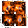 |
Fig. 1 Anticorrelation between N2H+ and C18O. Color background: N2H+ (1–0) emission integrated over all seven hyperfine components. The noise in these maps is σ = (0.030, 0.027, 0.025, 0.029) Jy beam-1 km s-1 for IRAS4A, L1448C, L1157, and IRAS4B, respectively. The wedges show the N2H+ intensity scale in Jy beam-1 km s-1. For the two lower panels the scaling is the same. Contours show emission of C18O (2–1) in steps of 6σ (IRAS4A) or 3σ (L1448C, L1157, and IRAS4B), starting at 3σ, with σ = (0.044, 0.029, 0.031, 0.033) Jy beam-1 km s-1 for IRAS4A, L1448C, L1157, and IRAS4B, respectively. The inlays in the upper right corners show the methanol emission as color background and contours in steps of 3σ, starting at 3σ inside the central 2′′, with σ = (0.028, 0.019, 0.027) Jy beam-1 km s-1 for IRAS4A, L1448C, and IRAS4B. In L1157, the methanol line has not been detected at a 3σ level. The filled ellipses in the lower left corner of the panels indicate the synthesized beam sizes of the N2H+ observations at 3 mm. The dashed white lines illustrate the small-scale outflow directions (see Table 3 and Sect. 3.1), and the white crosses show the positions of the sources as listed in Table 1. |
Results of elliptical and circular Gaussian fits in the uv plane to the C18O emission integrated over ±3 km s-1, performed with task uv_fit in MAPPING.
L1157
L1157-MM is a young Class 0 protostar in the L1157 dark cloud. The distance is rather uncertain and could be 250, 300, or 450 pc (Kun 1998; Looney et al. 2007). L1157-mm is driving the prototype of a so-called chemically rich outflow. Its outflow is characterized by a series of blue- and redshifted bow shocks interpreted as the impact of the precessing jets with the slow ambient medium and/or the outflow cavities (e.g., Bachiller & Pérez Gutiérrez 1997; Bachiller et al. 2001; Codella et al. 2010). The mean PA of the CO outflow is reported as 161° (Bachiller et al. 2001), and models suggest a jet precession cone of 15° opening angle (Gueth et al. 1996; Zhang et al. 2000; Bachiller et al. 2001). The jet is detected only within 10′′ of the protostar (Tafalla et al. 2015) and its direction has been recently measured as part of the CALYPSO project (Podio et al. in prep.). The envelope mass and the luminosity of this protostar were estimated as 1.5 M⊙ and 4.7 L⊙, respectively, by Kristensen et al. (2012), assuming a distance of 325 pc. The internal luminosity derived from the Herschel 70 μm flux is 3.9 L⊙. To be consistent with the work of Kristensen et al. (2012), we adopt their values.
3.2. Emission morphology
Figure 1 shows the observed integrated emission of C18O, N2H+, and CH3OH, where the lines of C18O and CH3OH were integrated over ±3 km s-1 around the systemic velocity of each source (see Table 1), while the emission of N2H+ was integrated over a window of 20 km s-1 that covers all the hyperfine components of the (1−0) transition. We derived the systemic velocities for the sources from an inspection of the C18O spectra extracted at the source position. This procedure might be prone to uncertainties because of the unknown dynamics of the inner envelope. Our analysis, however, does not depend on the exact values of the systemic velocities because we only use spectral information integrated over the full line width. We note that the intensity ratio of the N2H+ hyperfine lines, fitted with CLASS and averaged within the central 10′′ towards IRAS4B, IRAS4A, L1448C, and L1157, is 3:5:1.3, 3:4.6:1.4, 3:4.9:1.8, 3:5.1:1.1, respectively. These ratios suggest that the emission in the central regions is, on average, optically thin, where the ratio would be 3:5:1.
C18O morphology: in IRAS4B and L1157, the emission of C18O is clearly elongated in the direction of the outflow, while for IRAS4A and L1448C the influence of the outflow on the C18O is less clear. In the case of IRAS4A, the emission is elongated both along the inner outflow PA (north-south) and towards IRAS4A1 in the southwest. However, it still clearly peaks on A2, consistent with this COM source being the main heating source (see Santangelo et al. (2015)). In L1448C, the emission region is elongated almost perpendicular to the outflow, unlike in the other sources.
N2H+ morphology: for all four sources, we clearly resolve the expected rings of N2H+ emission around the region where CO is sublimated. Peaks of N2H+ are found in regions roughly perpendicular to the outflow direction. These peaks closely adjoin the C18O emission, strongly suggesting that the C18O and N2H+ emission extents in a direction perpendicular to the outflow are dominated by CO and N2 ice sublimation. The N2H+ rings are perturbed along the outflow axis. The N2H+ abundance is indeed expected to decrease in shocks along the outflow owing to electronic recombination (e.g., Podio et al. 2014). An interesting case is IRAS4A, where the N2H+ emission seems to drop along the direction of the large-scale outflow at a PA of ~45°. The outflow direction changes about 10′′ away from the central source (Yıldız et al. 2012), which corresponds to a timescale of ~600 yr. The observed N2H+ “hole” at PA = 45° also coincides with the EHV peak in the A1 outflow seen by Santangelo et al. (2015, right panels in their Fig. 5). A somewhat puzzling case, in terms of its emission in N2H+, is L1448C. Contrary to the other sources, the peaks in N2H+ emission are not equidistant to the central source and one of them does not closely adjoin the CO emission.
CH3OH morphology: compact methanol emission in the CH3OH (51–42) transition is seen in all sources, except L1157. In IRAS4B, there is some additional emission ~4′′ north of the continuum emission peak along the N-S outflow direction.
Results of elliptical and circular Gaussian fits in the uv plane to the CH3OH emission integrated over ±3 km s-1, performed with task uv_fit in MAPPING.
3.3. Size measurements
To determine the extent of the emission regions of C18O and CH3OH, we performed Gaussian fits in the uv plane, where we averaged the spectral channels over ±3 km s-1 around the systemic velocity of each source. So as not to be too much influenced by the irregularities in the emission morphologies, we fixed the centroid of the fits on the source positions.
The elliptical fits of C18O confirm the elongation along the outflow axis within 15° for all sources except L1448C (see Table 3). Because we want to exclude the perturbing influence of the outflow to probe only the effect of source heating, we also performed fits with the orientation of the ellipse fixed along the outflow directions at the respective PA, as found in the literature (see Sect. 3.1 and Table 3). For IRAS4A, we used the small scale value of PA = 0° which also excludes the interfering influence of IRAS4A1. For L1448C we used a PA of 160°, which corresponds to the orientation of the red-shifted component (Hirano et al. 2010). Finally, for comparison, we also performed circular Gaussian fits, even though this source model apparently does not match the observed morphology of the sources at all.
If we take the values obtained from fits with fixed major axis as being the most reliable fits to trace the “unperturbed” extent of the CO emission, the fitted half width at half maximum (HWHM) along the direction perpendicular to the outflow varies between ~280 and ~560 au in our sources. Based on the luminosity values from Table 1, the size of the emission region grows with higher luminosity, as expected if CO ice is sublimated mainly by radiative heating by the central source.
However, we advise that the values derived from elliptical Gaussian fits in the uv plane need to be taken with some caution. From the emission maps shown in Fig. 1, it is already apparent that the model of an elliptical Gaussian source morphology does not come close to the rather complex emission we see in our high angular resolution data. Accordingly, the complex source morphology adds an additional source of uncertainty to the fits beyond the formal error from the fitting procedure itself, as reported in Tables 3 and 4. Plots of the radially averaged uv data of the C18O emission can be found in Appendix B.
The compact methanol emission looks better suited to be fitted by elliptical Gaussians than the rather complex emission in C18O. However, here too the influence of the outflow together with a low signal-to-noise ratio in IRAS4B and L1448C challenge the quality of the fits. Especially in IRAS4B, the observed methanol emission is strongly affected by the outflow in the form of an extended pedestal, therefore the uv fit does not reliably trace the CH3OH snow line, as can be seen from the large eccentricity of the fit along the outflow (see Table 4). This problem also affects the trustworthiness of the fit with fixed PA. The fits for IRAS4A and L1448C show the uv-fitted Gaussian radius of the CH3OH emission zone at ~140 and ~50 au, respectively. We note, however, that these fits already operate at the limiting scale of our angular resolution and should accordingly be also treated with some caution for that reason. Among the sources, IRAS4A is expected to be best suited for tracing the methanol snow line, due to its high luminosity and the high signal-to-noise ratio in the methanol transition, even though the PA and the eccentricity of the fit hint at an influence of the outflow that is also in this source. Plots of the radially averaged uv data of the CH3OH emission are shown in Appendix B. It may be interesting to compare our methanol observations with observations of H O, obtained by Jørgensen & van Dishoeck (2010c) and Persson et al. (2012). Their observations, also performed with the PdBI, have synthesized beam sizes of 0.67′′× 0.5′′ and 0.86′′× 0.70′′ for IRAS4B and 4A, respectively. The authors find extents of the water emission regions of 0.2′′ and 0.6′′ (FWHM values of Gaussian fits) in 4B and 4A. Accordingly, we see a methanol emission region in IRAS4A that is twice the size of the cited water observation.
Finally, how does the HWHM of Gaussian fits to the observed emission regions relate to the corresponding snow line? The snow line marks the radius at which a particular species starts freezing out onto the dust grains (for a more technical definition, see Sect. 5.3). With respect to the abundance profiles, we theoretically expect three different regions: the central region where all molecules are in the gas phase, a transition region right outside of the snow line, where the molecules are partly depleted, and the outer region, where all the molecules are found as ice on the surface of the grains. Inside the snow line, the gas-phase abundance is roughly constant, but the density and temperature both increase as power laws towards the central source. Accordingly, the line brightness also strongly increases towards the center, and the emission radius at half-maximum, as measured by Gaussian fits, is expected to be smaller than the true extent of the snow line. How close the observed HWHM of the emission region comes to the radius of the snow line depends on various factors, like the width of the transition region, the temperature and the density profiles, and the observing beam. Thus, to derive a reliable estimate of the location of the snow line from the uv-fitted HWHM or the full observed intensity profiles, chemical and radiative transfer modeling, and a proper simulation of beam smearing by the PdBI interferometer, are required.
4. Analysis
4.1. The model
We aim to reproduce the observed emission in N2H+, C18O, and CH3OH using a chemical model with the envelope density and temperature structure of the respective source, coupled with a simple radiative transfer model. We vary the binding energies of CO and N2 ices and their abundances to fit the observed sizes and intensities in C18O and N2H+.
As input for the chemistry model, we use the 1D density and temperature profiles published by Kristensen et al. (2012). They assume that the density profiles follow a power law with n ∝ r− p. The inner boundary of the model is set at a radius where the dust temperature is 250 K. Using the DUSTY envelope model, the power-law index p of the density models was constrained for each source using the radial dust emission profiles of 450 and 850 μm SCUBA observations, which trace the outer envelope. In the production of the radial emission profiles, regions around the source that show irregularities, like other sources or bad data, were excluded. The spectral energy distributions of the sources as compiled from the literature were used to determine the extent of the envelope and the dust optical depth at 100 μm. The model parameters for our sources are listed in Table 5. We assume that the gas and the dust have the same temperature, which is justified at the high densities considered (which are ~103 cm-3 in the outermost envelope and a few 109 cm-3 in the center).
Model parameters.
Based on these density and temperature profiles, we used the Astrochem chemistry code (e.g., Maret & Bergin 2015) to determine the chemistry in the envelopes of our sources. This code computes the abundances of chemical species as a function of time for a stationary, spherically symmetrical source structure, where each shell of the source is at constant density and temperature. The code accounts for gas-phase reactions, cosmic-ray and photo ionization, and photo-dissociation, as well as for gas-grain interactions, namely H2 formation on grains, electron attachment and ion recombination, depletion, and desorption processes. We assume a standard value for the cosmic ray ionization rate of 1.3 × 10⁻¹⁷ s-1. The dust grain abundance relative to H2 that we use in our model is Xd = 2.6 × 10⁻¹², which corresponds to a nH2 to nd ratio of 3.79 × 10¹¹. The average grain size is 0.1 μm, so that the assumed gas-to-dust mass ratio is 100. The average grain size and the grain abundance we use is chosen such that it gives the same total grain surface area per H nucleus as an MRN distribution.
We use a chemical network containing gas-phase reactions and rates from the Ohio State university (OSU) astrochemistry database in its 2009 version with updated nitrogen reaction rates, as published in Daranlot et al. (2012). Binding energies and reaction rates for the grain-gas interactions were taken from Garrod & Herbst (2006), Öberg et al. (2009b,a), Bringa & Johnson (2004). For the CO and N2 ices, in particular, we initially assume multilayer desorption of pure ices and corresponding binding energies of 855 K and 790 K, respectively (Öberg et al. 2005). We further assume that methanol desorbs at the same temperature as the water ices, since its desorption behavior, being classified as a “water-like species”, is assumed to be dominated by hydrogen-bond interactions with water (Collings et al. 2004). This corresponds to an assumed binding energy for methanol of 5700 K. However, we note that this value constitutes an upper limit, as methanol may also be contained in CO dominated ices, see the discussion in Sect. 5.5. The values of the binding energies determine the size of the respective emission regions, because they determine the dust temperature at which the freeze-out of gas-phase species occurs. Given that the exact value of the binding energies depends on the (unknown) composition of the ices, they are used as free parameters to adjust the modeled emission sizes to the observed ones. We follow this approach in Sect. 4.2. However, we will not attempt to adjust the CH3OH binding energy, since the observed emission sizes in this species appear too uncertain and affected by outflow contamination.
The adopted elemental abundances correspond to the “low metal case” from Wakelam & Herbst (2008), but with a slightly lower oxygen elemental abundance of 3.2 × 10⁻⁴ relative to H2, following Hincelin et al. (2011). Our chemical initial conditions include six molecules: H2, NH3, CO, N2, CH3OH, and H2O. Except for H2, the molecules were initially put into ices, because the thermal desorption timescale is much shorter than the depletion timescale inside of the snow line (see, e.g., Fig. 7), and therefore the molecules return quickly to the gas phase in that region. To keep the number of free parameters small, we only vary the initial abundances of CO, N2, and CH3OH to match the observed line-peak intensities. In all the models, we include, somewhat arbitrarily, 10% of the elemental nitrogen abundance in NH3 ices. This value is in line with a total fraction of nitrogen locked up in ices of up to 10%–20% as found by Bottinelli et al. (2010). The oxygen that is not bound in CO and CH3OH is put in water ice. The water abundance will thus be overestimated, given that we do not include CO2 in the initial chemical conditions so as not to introduce another unknown parameter in our model. This should not have a critical effect on our modeling results of the CO emission, because most of the CO emission stems from a region where water is still bound in ice. By varying the initial water abundance, we also checked that the more compact methanol emission is not affected by the assumed water abundance (see Appendix C).
We stop our chemical models at a time of ~5 × 10⁴ yr, hereafter referred to as the chemical age. We note that for CO, the adaption of the initial CO abundance to match the observed intensity is straightforward, since in the central region basically all CO that is initially put into CO ices is finally found in the gas phase with little change over time. For N2H+, we matched the peak intensity found at the ring radius, but here we find a slight time dependence since N2H+ is destroyed over time. For methanol, the final abundance depends rather strongly on the assumed chemical evolution time, because methanol strongly participates in chemical reactions once it is in the gas phase. Appendix C shows the computed abundance profiles for several chemical ages.
We stress that the comparison between our model and the observations will only constrain the present-time peak values that are fed into the radiative transfer routine. They cannot however constrain the initial abundances since the inference to the initial abundances from the observed emission depends on unknown parameters, like the chemical age or the specific chemical composition of the gas. In Table 5, we list our best determined parameters, namely the plateau or peak values of the present-time abundance profiles of C18O, N2H+, and CH3OH that are obtained as outputs of Astrochem and then used to compute the emission maps that best reproduce the observations.
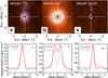 |
Fig. 2 Top row: comparison of the observations (contours) with the synthetic maps (color background) produced by the best fit model for IRAS4B with Eb(CO) = 1200 K and Eb(N2) = 1000 K. Top left: C18O (2−1), center: N2H+ (1–0), right: CH3OH (51−42), integration intervals are the same as in Fig. 1, while the contour spacing is in steps of 3σ, starting at 3σ. The white dashed lines show the outflow direction, while the dotted lines show the direction of the intensity cuts. The scaling of the maps can be understood in comparison with the cuts in the bottom row. Bottom row: cuts perpendicular to the outflow direction (PA = 0°) for C18O, N2H+, and CH3OH (left to right). Gray lines show the data, red lines the model. The blue bars in the top right corners of the bottom panels show the HPBW along the cut. |
For the sake of information, we have however also listed all initial abundances that we used in Astrochem to model our four sources in Table D.1. We stress that the fitted central methanol abundances as listed in Table 5 are to be understood as upper limits, given that the modeled Gaussian size (assuming a binding energy of 5700 K) is generally much smaller than the observed uv-fitted size.
The resulting abundance profiles are finally fed into the radiative transfer code RATRAN (Hogerheijde & van der Tak 2000). This code computes the molecular excitation and the resulting molecular line emission based on the Monte Carlo method for an axially symmetric source model. In our computations, we assume no radial velocity gradient and a 16O/18O isotopic ratio of 500, consistent with the value of 479 ± 29 found by Scott et al. (2006). The Doppler parameter for each source is chosen to match the width of the C18O lines. The corresponding values are listed in Table 5. The molecular data that is needed in the computation of the excitation characteristics is taken from the Leiden Atomic and Molecular Database and include collisional rates from Yang et al. (2010), Schöier et al. (2005), Daniel et al. (2005), Rabli & Flower (2010). For C18O, where different collision rates exist for ortho- and para-H2, we assume that collisions with ortho-H2 dominate in the high temperature regions where the observed radiation originates. Given that we observe optically thin emission in N2H+ (see Sect. 3.2), we calculate all hyperfine components separately and then add the intensities of the components.
From the resulting images we then compute uv tables with the GILDAS mapping software, using the same uv coverage as in our observations. Therefore, the effect of missing short spacing information that filters out the large-scale envelope structure in the observations is compensated for in the model and the potentially disturbing influence of large-scale emission from the colder envelope is prevented. Subsequently the same imaging and image deconvolution steps are applied to both the observed and the modeled uv data. To bring the model in accordance with the observations, the initial molecular abundances of CO, N2, and CH3OH are used as free parameters (varied in steps of the first decimal place of the abundance) to match the observed peak intensities, while the binding energies were varied (in steps of 100 K) to match the observed emission size in the uv plane and the observed intensity cuts of the spatially resolved emission. For the optimization no automated grid approach was used but the matching between model and observation was done by eye. Appendix C illustrates the impact of changes in the CO binding energy, as well as the impact of the initial CO abundance on the resulting chemical abundance profiles.
4.2. The testcase: IRAS4B
IRAS4B is the source with the least disturbed anti-correlation pattern in C18O and N2H+. Furthermore, it seems to be a single source with relatively simple continuum and C18O emission morphologies. Therefore we take this protostar as a test case on which we adjust and explore our modeling approach.
If we just run the chain of models as described in Sect. 4.1 on the envelope structure of IRAS4B, we obtain a C18O emission region that is clearly more extended than our observations. A Gaussian fit in the uv plane of the resulting synthetic observations yields a minor axis (FWHM) in East-West direction of 5.3′′, more than twice the fitted size of the observation. The predicted intensity cuts perpendicular to the flow are also twice too broad.
The radius where CO starts freezing-out on grains depends on mainly two different factors: the temperature profile of the source model and the CO ice binding energy. A decrease of the temperature profile would reduce the size of the CO emission region but it would also decrease the size of compact methanol emission. We discuss this scenario, which links back to possible uncertainties in the source luminosity, in Sect. 5. Here we only note that the C18O morphology in IRAS4B could be reproduced with temperature and density profiles divided by a factor of 1.5 compared to the profiles published by Kristensen et al. (2012). However, in the following we adapt the CO binding energy to match the observed emission regions.
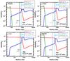 |
Fig. 3 Fractional chemical abundances, relative to H2, of C18O (red lines), N2H+ (blue lines), and CH3OH (green lines), computed by Astrochem for the envelope structures of IRAS4A (top left), L1448C (top right), L1157 (bottom left), and IRAS4B (bottom right). The light gray dotted lines show the HWHM of the modeled emission, the dark gray dotted lines the HWHM of the observed emission in C18O (see Table 3), while the light blue dashed line shows the location of the CO snow line in the model (see Table 5). The figure also indicates the dust temperature values at the respective radii. In IRAS4B, the observed and modeled HWHM are the same. |
The value of the CO binding energy we initially use in the model is 855 K (Öberg et al. 2005). We can reproduce the observed emission size in our model if we increase that value to 1200 K. In Fig. 2 we also compare the model and the observations in the image domain where, in the upper panel, the observations are overlaid as contours on the model as color background. For better comparison, the lower panel shows intensity cuts from model and observation perpendicular to the outflow direction. The cuts are seen to agree very well.
The match of the N2H+ ring also requires an adaption of the N2 binding energy, because the size of the ring depends on that parameter. While the inner radius of the ring is set by the desorption of CO into the gas phase and corresponding destruction of N2H+, the outer radius of the ring is set by the freeze-out of N2 ices and thus by the N2 binding energy. If we use a value of 1000 K, we obtain a very good match between the synthetic and the observed ring perpendicular to the outflow axis. The only shortcoming is that our model still shows some emission towards the center. Figure C.1 shows that this is not a time-dependent effect. It rather seems like our model misses some mechanism to destroy N2H+ in the innermost envelope. As well as by CO, N2H+ is also destroyed by water, CO2, and free electrons. However water is released from ices only in the innermost regions, as confirmed by the small H2O sizes observed in two of our sources, and this effect is already included in our model. At the same time, all the oxygen is bound in CO and H2O in our model. Accordingly we do not account for the effect of N2H+ destruction by CO2 via proton transfer, which occurs in a larger region than the destruction by H2O owing to the lower binding energy of CO2 ices compared to water ices. In addition, destruction by free electrons may probably be at work. These could either be created by uv radiation stemming from the central protostellar object and penetrating into the inner envelope inside of the outflow cavity (e.g., Visser et al. 2012), or, if present, by X-rays in the innermost region (e.g., Stäuber et al. 2007; Prisinzano et al. 2008). In the framework of our modeling approach, we are however unable to disentangle these possible effects.
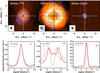 |
Fig. 4 Same as Fig. 2, but for IRAS4A. The cuts are performed at a PA of 90° perpendicular to the outflow direction (PA = 0°). |
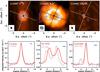 |
Fig. 5 Same as Fig. 2, but for L1448C. The cuts are performed at a PA of 70° perpendicular to the outflow direction (PA = 160°). |
In the case of methanol, the comparison between model and observation in the uv plane is hindered by the outflow contamination of the observations and by the resulting problems to apply a Gaussian model. Therefore we refrained from attempting to fit the observed size with a modified methanol binding energy and kept the same value of 5700 K as for water ices. The model fit yields a FWHM of 0.2′′ for IRAS4B. This is much smaller than the average FWHM of complex organic molecule emission in this source of 0.5 ± 0.15′′, as we observe it in our WideX spectra (Belloche et al. in prep.). In the image domain, model and observation have the same intensity profile corresponding to the beam (see Fig. 2), but this merely illustrates that the modeled and actual emission sizes are smaller than the beam size.
The underlying chemical abundances of the model shown in Fig. 2 are presented in the lower right panel of Fig. 3. As outlined in Sect. 3.3, the abundance profiles of C18O and CH3OH show an inner plateau region, a transition region, and an outer region of depletion. The transition from complete depletion to the maximum gas-phase abundance happens within a few hundred au for CO and about ten au for methanol. The initial abundances of CO, N2, and CH3OH are adjusted to match the observed peak intensities (see Tables 5 and D.1). This procedure yields an inner abundance of C18O of about 3 × 10⁻⁸, which corresponds to an inner abundance of C16O of 1.7 × 10⁻⁵ relative to H2. The fitted central methanol abundances as listed in Table 5 should be understood as an upper limit, since the modeled CH3OH Gaussian size is much smaller than observed. If the real extent (and beam filling-factor) of the methanol emission is larger than in our model, the required abundance to match the observed flux would be lower.
In this model, the C18O and methanol snow lines, where the respective desorption and depletion rates are equal and where the plateau abundances start dropping, are located at radii of about 460 au and 35 au, respectively. The N2 snow line is found at a radius of 760 au. In Fig. 3, the CO snow line radius is indicated as a light blue dashed line, together with the dust temperature at this location, which is ~24 K. The HWHM radii of the observed and modeled C18O emission, as inferred from Gaussian uv fits, are also shown as dark gray and light gray vertical dotted lines, respectively. They are identical in IRAS4B, hence superimposed on this graph. The corresponding dust temperatures are also indicated. It may be seen that the HWHM is substantially smaller than the true CO snow line radius, by a factor 1.6. Hence, the uv-fitted HWHM of C18O only gives an upper limit to the freeze-out CO dust temperature of 30 K instead of 24 K in the present case. The angular radius of the CO snow line in IRAS4B (about 2′′) corresponds more closely to the radius at zero intensity of the C18O intensity cut. However, this coincidence may not hold for all sources or species. For example, the modeled angular radius of the N2 snow line in IRAS4B (about 3′′) falls closer to the half-maximum of the N2H+ emission cut than to its radius at zero intensity (5′′). This is because the intensity profile will depend not only on the snow line location, but also on the width of the transition region and on the residual abundance outside of it.
4.3. The other sources
For the other three sources, we used the same values of the binding energies for CO and N2 as were found to reproduce the emission of IRAS4B. The chemical abundance profiles are shown in Fig. 3, and the modeled emission for the three sources is presented in Figs. 4−6. In all sources, the emission intensity profile of C18O is well reproduced, as well as the overall peak location and thickness of the N2H+ ring.
In IRAS4A, the size of the C18O emission obtained from Gaussian fits in the uv plane is a bit smaller for the model than the observed size (4.5′′ versus 4.8 ± 0.07′′). The match of the intensity cuts in the image plane is, however, satisfactory with an inner C18O abundance of ~2 × 10⁻⁸ relative to H2, which corresponds to an inner abundance of C16O of 9 × 10⁻⁶. The emission of N2H+ appears to be strongly disrupted by the influence of the precessing outflow, therefore it is difficult to evaluate the quality of the fit based on one single cut. In the cut displayed in Fig. 4, the synthetic observations do not fit the observations very well, but the edges of the emission ring, as well as the part of the ring at positive offsets, satisfactorily correspond to the modeled ring. We note that in this source, as well as in L1448C, the deconvolution of the modeled observations has to account for the fact that the first sidelobes of the synthesized beam have about the same size as the modeled ring emission. Therefore, in these two sources we have applied a ring-like support in the deconvolution of the models. This support influences the value of the image peak intensity. Accordingly, in these two sources, the N2H+ abundance is less well constrained. Again, the methanol emission is reproduced in the image domain at a size that corresponds to the beam size. In the uv domain, however, the modeled emission FWHM size is much smaller than the observation (0.44′′ versus 1.2 ± 0.06′′).
In L1448C, the intensity cut of the C18O emission regions of the model and the observations agree satisfactorily in the image domain perpendicular to the outflow (Fig. 5). The model in N2H+ underscores the rather strange observed morphology, where the emission peaks are not equidistant to the central source: model and observations seem to be shifted with respect to one another, even though the width of the emission region, as well as the spatial distance between the peaks seem rather well reproduced. The inner C18O abundance in L1448C is found to be ~2 × 10⁻⁸ relative to H2, which corresponds to an inner abundance of C16O of 10-5. The modeled emission FWHM size for methanol is 0.33′′, which lies within the error bars of the observed FWHM perpendicular to the outflow of 0.37 ± 0.13′′.
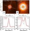 |
Fig. 6 Same as Fig. 2, but without methanol, for L1157. The cuts are performed at a PA of 71°, perpendicular to the outflow direction (PA = 161°). |
For L1157, the match between model and observations in C18O and N2H+ is also satisfactory. The distance between the N2H+ maxima is a bit smaller in the model than for the observation. On the other hand, the modeled C18O emission is a bit more extended than the observed emission. L1157 has the highest inner C18O abundance of the four sources with a value of 6 × 10⁻⁸ relative to H2, which corresponds to an inner abundance of C16O of 3 × 10⁻⁵.
Figure 3 shows the chemical abundance profiles for all sources, which are similar in all cases. As already described in Sect. 4.2, in the case of IRAS4B, the HWHM derived from the Gaussian fit of the C18O observation in the uv plane (shown as dark gray dotted lines) is significantly smaller than the snow line radius (light blue dashed line) in all sources. Notably, this also holds for the relation between the radius of the snow line and the HWHM of the modeled emission, which is a factor of 1.5−2 smaller than the snow line radius.
We finally note that we also applied our model to IRAM 04191, to check whether the locations of the outer and inner radii of the N2H+ ring correspond to the radii of CO and N2 freeze-out. If we use the temperature and density profiles presented in Belloche et al. (2002), according to our model the peak of the N2H+ ring should be located at a radius of ~100 au, while the observations show the ring at a radius of ~1400 au, assuming a distance to IRAM 04191 of 140 pc. Using the same CO and N2 binding energies as for the other sources, the observed ring can only be reproduced with a temperature profile that is three times higher than derived in Belloche et al. (2002). The observed, weak, compact C18O emission, however, does not fill the large N2H+ ring, as would be expected if the ring is the result of a chemical anti-correlation. Accordingly, these observations call for further investigation and may suggest that, provided the temperature and density profiles are correct, the N2H+ ring in IRAM 04191 hints at a different situation than in the other four sources (see also Belloche & André 2004). It might, for example, be related to a past accretion burst. We will discuss this source in a forthcoming paper.
5. Discussion
As was shown in Sect. 4, our model is able to reproduce the observed emission well in all four sources if we increase the CO binding energy to a value of 1200 K and the binding energy for N2 ices to 1000 K. The observational fact that the CO emission is less extended than expected with the initially assumed binding energy for pure CO ices contradicts a scenario where the chemistry traces a past accretion burst (e.g., Visser et al. 2015). Furthermore, we note that in all cases, we need very low CO abundances compared to the general dense ISM (where typical values of the CO abundance in molecular clouds are ~0.6−2 × 10⁻⁴, e.g., Ripple et al. 2013) to reproduce the peak intensities. In this section, we first address general uncertainties in our modeling approach, before we discuss in more detail our findings on the CO binding energy, the CO freeze-out temperature, the N2 and the methanol binding energies, and the CO abundances. Finally we briefly compare our findings with a recent study of the CO snow lines in three of our objects by Jørgensen et al. (2015).
5.1. Uncertainties in our modeling
Our modeling relies on a number of assumptions. One major ingredient is the adopted temperature and density profiles that were derived by Kristensen et al. (2012). To stay consistent with their modeling, we used the same values for source distances, luminosities, and envelope masses that they assume in their work.
Uncertainties in the source luminosities translate into an uncertainty of the temperature profiles. With a different temperature profile, the same observed position of the snow line would result in a different binding energy. In particular, Fig. 4 of Jørgensen et al. (2015) shows that we could reproduce our observations with a lower value of the CO binding energy of 855 K if the luminosity was a factor of 4 smaller than the values we assume in our analysis. The uncertainties in the luminosities reported in Sect. 3.1 for L1448C and L1157 are clearly smaller than this factor of 4. Accordingly, the modeling of our observations always requires for these two sources a higher binding energy of CO than the value of multilayer desorption for pure CO ices within the range of uncertainties in source luminosity. However, as mentioned in Sect. 3.1, the internal luminosities of IRAS4A and IRAS4B derived from Herschel 70 μm data are 3.4 L⊙ and 1.5 L⊙, respectively, which are a factor of ~3 smaller than the bolometric values we use in Sect. 4, derived by Karska et al. (2013). If the Herschel internal luminosities were used, we would need to assume a lower CO binding energy in IRAS4A and 4B than in L1448C and L1157, implying a different ice composition. We note that adopting bolometric luminosities for all sources, as we have done, gives equal CO ice-binding energies for all of them.
The temperature profiles are also subject to other uncertainties beyond variation of the source luminosity only. In their paper, Kristensen et al. (2012) do not provide estimates for these uncertainties, but in a detailed description of their modeling3 they exemplarily show for a Class I source that the temperature profiles as a function of radius are very robust with respect to changes in the power-law density slopes, and variations in the sub-mm and mm fluxes at radii larger than ~100 au. The uncertainty in the temperature profiles, however, grows strongly for smaller radii. Accordingly, while the determination of the CO freeze-out temperature that is reached at radii of a few hundred au should be rather robust (given the luminosity values are basically correct) the uncertainty is larger for the determination of the inner CO abundance, which is affected by the innermost temperature structure and corresponding excitation characteristics.
It is important to note that a different temperature profile, contrary to a change of the CO binding energy, will also affect the size of the methanol emission region. In IRAS4A, the source with the most reliable uv fit of the methanol emission region, we observe a FWHM of the emission region of 1.2 ± 0.06′′. With the temperature profile from Kristensen et al. (2012), this FWHM value would hint at a freeze-out temperature for methanol of less than 70 K, which already seems unreasonably low given laboratory measurements (e.g., Collings et al. 2004 who find a binding energy for methanol on water ice of 5530 K, which corresponds to dust temperatures of ~120 K). A reduced temperature profile would decrease the dust temperature at the observed HWHM even further. However, we have to stress again that the uncertainty of the temperature profile increases strongly in the central region of the envelope where methanol is present in the gas phase, such that the use of methanol for probing the adopted temperature profile might be rather questionable, all the more so since the influence of the outflow on the methanol emission might dominate the effect of source heating (see Sect. 5.5).
There is another uncertainty regarding the distance of L1157, where we use a value of 325 pc, which is larger by a factor of 1.3 than the value of 250 pc that is used, for example, by Codella et al. (2015) and Podio et al. (in prep.). However, the variation of the temperature in the envelope as a function of the angular size should be independent of the assumed distance. This can be seen from Eq. (2) of Motte & André (2001), which says that the temperature in the envelope, as a function of its radius, is proportional to (L⋆/r2 )0.2. Because the luminosity L is given as the product of the observed stellar flux times the distance squared, and the radius r is proportional to the distance times the angular size, the distance dependence cancels out in the cited equation.
Another simplification in our model concerns the initial abundances adopted in Astrochem. While we use the so-called low metal case from Wakelam & Herbst (2008) for the metals, we put all the carbon in CO and methanol ices and all the nitrogen in N2 and NH3 ices. The CO and N2 ice abundances are then treated as free parameters. This is a situation that does not correspond to the chemistry we find in dark clouds where, for example, we also find nitrogen in the form of atomic N (e.g., Maret et al. 2006; Daranlot et al. 2012). Accordingly, as already described in Sect. 4.1, while we give the initial abundances we use in Astrochem in Table D.1 for the sake of completeness, the more significant information lies in the abundance profiles that are used in Ratran and that reproduce our observations (see Table 5).
The simplifications in the initial abundances, together with the fact that we use a stationary model, also suggest taking the chemical age of our models with some caution. Theoretically, an upper boundary of the evolution time is given by the assumed lifetime of the protostar. As another limiting factor, we find that methanol, once released into the gas phase, is converted by gas phase reactions (the dominant reaction beingH3O+ + CH3OH → CH5O+ + H2O), and its abundance is severely reduced in the center of the envelope, typically after about ~1 × 10⁵ yr. However, the fact that the envelope is collapsing with free-fall times at the radius of the methanol snow line of a few hundred years will prevent the effect of methanol destruction from becoming relevant as the envelope material is constantly replenished. Our stationary model does not account for the ongoing collapse, the computed chemistry is however not affected by the collapse, since it is dominated by the effect of ice sublimation that takes place on very short timescales inside of the snow line (see Fig. 7). An order of magnitude estimate of the effect of infall motions on the location of the snow line is performed in Sect. 5.3. Furthermore, we note that the computed abundance profiles of CO and N2H+ barely change up to a chemical age of ~1 × 10⁵ yr. Therefore we do not consider the exact chemical age of the models as being a crucial parameter for our modeling if it is below that value.
Another caveat of our model is the assumption of spherical geometry, although the observed sources deviate from this assumption owing to strong outflow activity and binarity, as we have discussed in Sect. 3.2. We account for this asymmetry by comparing observations and models in the direction that is perpendicular to the outflow direction. However, the models do not include the influence of the outflow cavities and related shock and PDR-like features on the excitation of the observed molecules. We note that including this extra heating would tend to broaden the predicted emission sizes. It would thus require an even larger ice binding energy to keep the emission size as small as observed.
5.2. The CO binding energy
Our models can reproduce the observations if we use a CO binding energy of 1200 K. This value is higher than the binding energies of pure CO ices. Laboratory studies differentiate on whether CO ices are located on top of water ices (monolayer desorption) or whether they are bound to a surface of CO ice (multilayer desorption). This differentiation can be understood in the framework of a simple onion model (e.g., Collings et al. 2003), where an inner hydrogenated, water dominated layer is surrounded by an outer dehydrogenated layer dominated by species like CO, CO2, N2, and O2. Accordingly, depending on the thickness of the outer layer, the CO ice is either separated from or directly bound to the underlying water ice, which results in different binding energies and desorption at different temperatures.
However, a number of studies (e.g., Collings et al. 2003, 2004; Fayolle et al. 2011; Martín-Doménech et al. 2014) have pointed to the fact that the physics and chemistry of the desorption of CO ice layers on grains is more complicated than a simple onion model would suggest. Actually, several desorption features, seen at different temperatures, show that not only multi- and monolayer desorption play a role in the release of CO from ices to the gas phase. Collings et al. (2003) argue that CO can get trapped in water ice. This is because of a phase change in the water ice component with increasing temperature, which changes the water ice’s structure from highly porous amorphous to a less porous amorphous phase. If CO diffuses into the porous structure of water ice at lower temperatures (see, for example, Lauck et al. 2015), this phase change may then prevent the CO from escaping through surface pores when the ice is heated. Only when the water crystalizes at even higher temperatures, does the trapped CO get desorbed in a process called molecular vulcano. A fraction of the CO that remains in the crystaline water layer is co-desorbed at even higher temperatures, together with the water. This behavior has been confirmed in experiments with precometary ice analogs (Martín-Doménech et al. 2014).
Our chemical model does not properly account for the complex layering of ices, but assumes that desorption takes place at a single temperature, as described by Eqs. (1) and (2). However, in locating the snow lines, which are the radii where CO starts freezing out, we are mostly interested in the dominant desorption processes that occur at the lowest temperatures. In the simplistic onion model, these would be multilayer (CO on CO) or monolayer (CO on H2O) desorption, depending on the thickness of the CO containing ice layer.
If we use an average grain size of 0.1 μm and assume 3 × 1015 cm-2 binding sites on the grains’ surfaces, the low gas-phase CO abundances in our sources (see Table 5) correspond to ~2 CO ice layers in IRAS4B and L1157 and ~1 layer in IRAS4A and L1448C. Of course these numbers strongly depend on the assumed average grain radius and on the actual layer structure of the grain ices. However, based on the above values, our models seem consistent with monolayer desorption of CO from water surfaces.
The measurement of the surface binding energies of molecular ices is usually performed using temperature programmed desorption, where ices are grown on a substrate in an ultra-high vacuum chamber. The substrate is then heated and the liberated gases are measured using a mass spectrometer. Using this technique, the binding energy of CO on CO was measured as lying between 850 and 1000 K (e.g., Sandford & Allamandola 1988: 960 K; Bisschop et al. 2006: 855 K; Cleeves et al. 2014: 855 K; Martín-Doménech et al. 2014: 890 K), while the binding energy of CO on an amourphous water surface is higher at values between 1200 K and 1700 K (Collings et al. 2004: 1150 K; Noble et al. 2012, coverage of 0.1: 1307 K, coverage of 0.2: 1247 K; Cleeves et al. 2014: 1320 K).
Indeed, the measured binding energies of CO ices on a water ice surface agree with what we require in our models. Alternatively, if the grain ices in our sources do not exhibit a clean layer structure, the CO binding energy could also be increased with respect to pure CO ices, if the CO ice is mixed with other polar ice components, such as CO2 and organic molecules. Cleeves et al. (2014) find a binding energy of 1100 K for CO on a CO2 surface, which is also close to the value we find. Indeed, the infrared CO and CO2 ice band shapes and correlations of CO/CO2/H2O ice columns across various lines of sights indicate that about 80% of CO ice in molecular clouds and towards young stellar objects is in a non-polar CO2:CO mixture (see Chiar et al. 1994; Pontoppidan et al. 2003, 2008; Pontoppidan 2006; Whittet et al. 2009). In addition, Penteado et al. (2015) argue for a gradient of ice mantle composition in grains around young stellar objects, where CO is mixed with CH3OH instead of water.
We conclude that, while our models seem consistent with monolayer desorption of CO from water ice surfaces, the structure of the grain ice layers may deviate from a clean layered structure where a pure CO layer sits on top of a layer of water ice. In any case, the value we derive for the binding energy of CO ices agrees well with laboratory measurements.
5.3. The CO freeze-out temperature
Observational studies often cite the freeze-out temperature instead of the binding energy. The relationship between the two values in our model, which is based on first-order kinetics, can be understood based on the underlying microphysics of the snow line. The snow line is located at a radius where the microphysical depletion rate equals the thermal desorption (Bergin et al. 1995; Hasegawa et al. 1992), which translates to 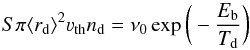 (1)with
 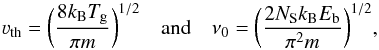 (2)where νth is the thermal velocity, S the sticking probability, which is taken to be 1, ⟨ rd ⟩ the average grain radius, nd the total grain density, Td the dust temperature, Tg the gas temperature, m the mass of the accreting species, and where ν0 is the characteristic vibrational frequency of the desorbing species with the binding energy Eb in Kelvin, and NS being the number of sites per unit surface.
From Eq. (1) it is apparent that the exponential in the binding energy is the dominating factor in determining the freeze-out temperature, as can also be seen in Fig. 7, which shows a plot of the timescales in the equation applied to the density and temperature profiles of IRAS4B. Even if the value of the thermal depletion rate is changed, e.g., by varying the total grain density by a factor of 10, the location of the snow line in terms of the dust temperature Td changes by less than 5%. Figure 7 shows that our best-fitting binding energy of 1200 K corresponds to a freeze-out temperature of ~24 K, which is in line with previous observations of protostellar systems.
Observations indicate that the freeze-out temperature of CO ices depends on the studied environments. Observations of more evolved proto-planetary disks find CO snow lines at lower temperatures of about 17 to 19 K, consistent with a binding energy of 855 K (e.g., Qi et al. 2011: 19 K, Mathews et al. 2013: 19 K, Qi et al. 2013: 17 K), observations of low-mass protostars yield higher values between 20 and 40 K, in line with our findings (e.g., Jørgensen 2004: 40 K, Yıldız et al. 2012: 25 K, Jørgensen et al. 2013: 30 K, Jørgensen et al. 2015: 30 K). Jørgensen et al. (2015) give a possible explanation of this difference in terms of grain ice growth. Because grains in disks around T Tauri stars may have been subject to heating and sublimation, the grains may have a clearer onion-like shell structure with a more purified CO ice layer than in protostellar environments, where different ices are probably formed simultaneously at low temperatures.
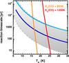 |
Fig. 7 CO ice depletion timescale (dark blue line) and thermal desorption timescales for binding energies of 855 K (orange line) and 1200 K (red line) as a function of the dust temperature for the density profiles of IRAS4B. The light blue line shows the free-fall time for an enclosed mass of 0.5 M⊙. The points of intersection at ~17 K and ~24 K indicate the locations of the CO snow line for the two different values of the binding energy. The gray area shows the range of depletion timescales if the dust density is varied by a factor of ten. For a binding energy of 855 K, the variation of the density translates into a variation of the snow line location at ~16 K or ~17 K, while for a binding energy of 1200 K, the modified snow line locations would be at ~23 K or ~25 K. |
Based on the desorption reaction timescale displayed in Fig. 7, we can also now obtain an estimate on whether the observed radius of the snow line could also be caused by infalling material with a binding energy of 855 K. This would be the case if the infall timescales are smaller than the desorption timescales. For a binding energy of 855 K, the desorption timescale at a radius of 1200 au where the dust temperature is 16 K is about 600 yr in IRAS4B. At the radius of the observed snow line at 460 au, this timescale has already decreased to about one hour. If we consider the free-fall speed from infinity onto a central mass,  , we can estimate the free-fall time at radius R as
 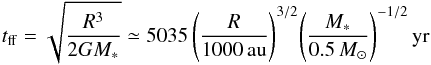 (3)with the gravitational constant G and the mass M∗ enclosed inside of radius R. Based on this formula4 with an estimated total enclosed mass of 0.5 M⊙, the free-fall time at the radius of 1200 AU, where the dust temperature is 16 K, would be ~7000 yr, more than an order of magnitude longer than the desorption timescale. In addition, the desorption time drops much more steeply with increasing dust temperature than the free-fall time, so even increasing M∗ by a factor of 2 would not modify the desorption temperature by a perceptible amount. The light blue curve in Fig. 7 shows the free-fall time for a constant enclosed mass of 0.5 M⊙, which is always longer than the desorption time inside the respective snow line, independent of the assumed binding energy. We conclude that the infall motion of the envelope will not have a significant impact on the location of the snow lines.
5.4. The N2 binding energy
To match the observed ring-like emission of N2 with our models, we had to assume an N2 binding energy of 1000 K. This value is also higher than values measured in the laboratory for pure N2 ices on N2 surfaces using temperature-programmed desorption. Again, the value of the binding energy depends on assumptions about the structure of the ices: if N2 forms an ice layer above the CO ice, it will get sublimated earlier than if it is contained in a mixed CO-N2 ice layer. In the latter case, the N2 binding energy would be close to the CO binding energy. Öberg et al. (2005) measured the binding energies of pure, layered, and mixed CO and N2 ices. They find that pure N2 ices have slightly lower binding energies than CO (790 ± 25 K versus 855 ± 25 K). In layered ices, the desorption kinetics are unchanged, but part of the N2 desorbs together with the CO because N2 diffuses into the CO ice. In a subsequent study, Bisschop et al. (2006) specify the binding energy of pure N2 ices as 800 ± 25 K. Our value of 1000 K agrees with the value measured for N2 ices on a compact water ice surface with at least 0.4 monolayers (Fayolle et al. 2016).
Öberg et al. (2005), as well as Bisschop et al. (2006), stress the important role of the ratio of the binding energies of N2 and CO ices for the reproduction of the observed anti-correlation by chemical models. It is intuitively clear that this ratio needs to be smaller than 1, because otherwise all the N2H+ is subject to destruction by CO if it is released only when CO is also present in the gas phase. For pure ices Öberg et al. (2005) and Bisschop et al. (2006) find a ratio of ~0.93, while for mixed ices the empirical value is lower at ~0.89. The importance of this ratio for the observed anti-correlation indicates that a change in the CO binding energy, as discussed in Sect. 5.2, may indeed imply an increase in the N2 binding energy. The ratio of binding energies used in this study, determined by fitting the ring of N2H+ emission in IRAS4B, is 0.83, which is lower than the above cited ratio for pure ices, but close to that expected for mixed ices.
5.5. The CH3OH binding energy
Among our four sources, only the Gaussian uv fits towards IRAS4A seems to reliably trace the size of the compact methanol emission because of the high signal-to-noise ratio, because IRAS4A is the only source where the peak of the emission is spatially resolved, and because the Gaussian fit to the methanol emission in the uv plane does not appear very much influenced by the outflow (The radially averaged uv data are shown in Appendix B.). The large uv-fitted size on IRAS4B is clearly measuring the size of the resolved pedestal along the outflow, not that of the central peak. Also the uv fit towards L1448C shows an apparent elongation along the outflow axis. In both sources, the peak of the methanol emission is not spatially resolved by our observations.
The fit of the methanol peak emission in IRAS4A in the uv plane yields a FWHM of 1.2 ± 0.06′′. This value corresponds to twice the size of the region, where water emission occurs, as observed by Persson et al. (2012) with a FWHM 0.61 ± 0.12′′. If both fits are reliable in tracing the sublimation regions without a significant influence of the outflow activity, this would hint at the (model-independent) interpretation that methanol has a lower binding energy than water. Indeed, laboratory studies find slightly lower values for the binding energy of pure methanol ices (e.g., Collings et al. 2004: 5530 K for methanol bound to a water ice surface vs. 5700 K for pure water, as well as water-methanol mixtures, which corresponds to dust temperatures of 120 K vs. 125 K in our sources). Furthermore, methanol is expected to also be present in CO-dominated ice when CO hydrogenation via H atoms on interstellar ice surfaces occurs (e.g., Cuppen et al. 2009).
If we want to derive a specific methanol binding energy from our observations, we however need to assume a model-dependent source temperature profile. If we take the temperature profiles of Kristensen et al. (2012), we find a freeze-out temperature of less than 70 K in IRAS4A based on our observations, which is much lower than the reported laboratory values. There are (at least) four different interpretations of this finding: 1. we see methanol co-desorbing from an ice environment with much lower binding energy than water ices like, e.g., CO dominated ices (see above); 2. the adopted temperature profiles are wrong at these small radii and the methanol binding energy is actually higher than indicated by the Kristensen et al. (2012) profiles (see Sect. 5.1); 3. non-thermal desorption at lower temperatures than the sublimation temperature may be efficient in releasing methanol into the gas phase; or 4. the influence of the outflow on the methanol emission is the dominating factor in determining the emission size and thus we cannot make statements about the methanol binding energy based on our observations. Because of these uncertainties, we refrained from properly fitting our observations with a modified methanol binding energy.
5.6. CO abundances
Typical ISM CO abundances in molecular clouds range from ~0.6–2 × 10⁻⁴ (Ripple et al. 2013 and references therein). Assuming a 16O/18O isotopic ratio of 500, this corresponds to a C18O abundance of ~1.2–4 × 10⁻⁷. In our models, we find inner CO abundances that are about one order of magnitude smaller than these values (see Table 5).
The CO abundances we find inside the CO snow line are lower than findings of most previous studies of protostars. Modeling IRAM 30 m observations of a sample of Class 0 protostars, Alonso-Albi et al. (2010) find the lowest value they consider as model input for the inner C18O abundance, 10-7, yielding the best fit of their observations. They however note that their fits would be even better with an even lower value. Yıldız et al. (2010, 2012) obtained observations of several transitions in C18O up to (10−9) towards IRAS2A, IRAS4A, and IRAS4B with the Herschel telescope and several ground-based single-dish observatories. Fitting these observations with a chemical jump model located at 25 K, they find inner C18O abundances of (1−3) × 10-7. These abundances are an order of magnitude higher than our values for the same sources.
However, we note that their inner C18O abundances are not very well constrained towards smaller values in their χ2 plots. Indeed, we have checked that our models for IRAS4A and 4B predict intensities that are consistent with those observed by Yıldız et al. (2012) up to J = 10−9. Hence, it appears that spatially resolved emission profiles of C18O, such as those obtained here with the PdBI, are essential to reliably constrain the gas-phase CO abundance inside the snow line. Using observations from the same group of observatories, Fuente et al. (2012) derive a central C18O abundance of 1.6 × 10⁻⁸ towards the young intermediate-mass protostar NGC 7129 FIRS 2, which harbors a hot core.
The low CO abundances are not restricted to the protostellar phase, they also seem to prevail in protoplanetary disks. Favre et al. (2013) used observations of HD in the TW Hya disk to probe the H2 mass in the warm gas at temperatures above 20 K. They find that the CO abundances in this warm molecular layer is reduced by at least an order of magnitude compared to dense clouds. They measure a disk-averaged warm gas-phase CO abundance relative to H2 of (0.1−3) × 10-5. Previous studies (e.g., Dutrey et al. 2003; Chapillon et al. 2008; Qi et al. 2011) had already described the very low CO gas-phase abundance in disks, however these earlier studies were not able to differentiate between the warm and the cold layers, and therefore could not exclude that the low value was due to depletion.
There are several scenarios that might explain these low CO abundances. One possible explanation could be that part of the CO is trapped in water ice and finally co-desorbs together with the water inside a region that is not resolved by our observations (see for example, Martín-Doménech et al. 2014 and Sect. 5.2). Alternatively, CO in grain mantles could be removed by reactions to form other species (e.g., Whittet et al. 2011). Observations confirm that a large part of carbon in the grain mantles can be bound in CO2 ices that have a higher binding energy than CO (e.g., Pontoppidan et al. 2008). Depending on the efficiency of gas-phase reactions that transform CO2 into CO once the ice is sublimated to the gas phase, carbon could thus also be “hidden” in CO2. Correlations of ice bands with Av show that the amount of CO and CO2 in ices are comparable up to 25 mag and are each, on average, 4 × 10⁻⁵ with respect to H2 (e.g., Whittet et al. 2007). Our CO gas-phase abundances of ~1−2.5 × 10⁻⁵ are still a factor 2–3 times smaller than this. Hence CO ice would need to be more efficiently channeled into other species inside protostellar envelopes than in dark clouds.
By using a detailed gas-grain chemical model for protoplanetary disk conditions, Reboussin et al. (2015) find that, at high densities, CO can indeed be efficiently converted in less volatile species like CO2. Possible other candidate products are CH3OH and CH4. Indeed, observations indicate that methanol ice abundances in low-mass YSO envelopes can reach 15−25% of water ice (Pontoppidan et al. 2008), similar to the CO ice abundance in less dense clouds (Whittet et al. 2007, 2009), while CH4 reaches 5% of the water ice (Öberg et al. 2008). Some of the missing CO could also be in the form of more complex organic molecules (e.g., Whittet et al. 2011). Two of the sources discussed in this paper, IRAS4A and IRAS4B, are well known hot corino sources that show a rich spectrum of COM emission lines. To properly investigate the relation between CO abundance and the existence of COMs, COM abundance measurements need to be performed for the sources of this study. In an upcoming paper (Belloche et al. in prep.), the CALYPSO project will study the COM emission in our sample of sources and may shed some light on their relevance for the problem of lacking carbon. However, the recent study by Taquet et al. (2015) on IRAS4A already indicates that the abundances of COMs are not high enough to solve the problem.
Finally, Aikawa et al. (1997) suggest a chemical mechanism in protoplanetary disks where X-rays from the central star produce He+ that can extract C from CO in the gas phase. Part of the carbon is then transformed into hydrocarbons or CO2. If X-rays are already produced in the Class 0 protostellar phase (which is not clear observationally, see e.g., Prisinzano et al. 2008), this explanation could also be relevant for the presented sources.
Given the small number of sources, it is obvious that more studies, particularly testing all the various scenarios that may explain the lack of CO independently, are necessary to settle the question on where the missing carbon is. In any case, it seems that the low CO abundances that are found in protoplanetary disks are already established in the protostellar phase.
5.7. Comparison with Jørgensen et al. (2015)
In a recent study, Jørgensen et al. (2015) analyzed the sublimation of CO, traced by emission in C18O (2–1), for a sample of 16 protostellar sources to trace variations of protostellar accretion rates. Their work has three sources in common with ours: IRAS4A, IRAS4B, and L1448C. Their findings, however, deviate from ours both with respect to the sublimation radii determined by uv fits of their observations and their modeling results. Their data was obtained with the SMA at an angular resolution of 2−3′′, which is about a factor of three worse than ours.
The elongation of CO emission along the outflow axis that we see in our data is not that apparent in their lower resolution data. The difference is particularly striking in the case of IRAS4B. This fact may already cause differences in the results of the uv fits, particularly as their observations can be fit satisfactorily by circular Gaussians, while these are not at all well-suited to fit our observations. Their fits are, however, consistent with our fits that are perpendicular to the outflow, if we take their maximum uncertainties of 0.5′′ and if we account for the fact that our elliptical fit of L1448C overestimates the extent of the emission in the image plane.
Regarding the applied modeling, there are clear differences between the two studies. In contrast to our modeling approach, they use a generic envelope model for all the sources. In particular, they apply a power-law density profile in all cases with a fixed exponent of 1.5 and vary the source luminosity. The density profile is normalized by comparison to single-dish submillimeter continuum observations. Based on each luminosity, they determine a self-consistent temperature profile. To determine a best-fit model for each source, they subsequently compare their observed CO maps with the modeled CO emission extent. With this procedure, they can then compare the luminosity that yields their best-fit model with the current observed luminosity. If the current luminosity is much smaller than the modeled one, they count it as a sign of a past accretion burst. For the freeze-out temperature they take a value of 30 K. The luminosity values they use differ from ours for IRAS4A and L1448C: 9.9 versus 9.1 L⊙ and 8.4 versus 9.0 L⊙, respectively. For the three sources, their modeled emission regions are clearly smaller than ours. This difference is easily explained, given their higher assumed freeze-out temperature.
Despite these differences, Jørgensen et al. (2015) agree with our findings in their conclusion that the sources we have in common do not show signatures of a past accretion burst. We however note that our sample includes one source, namely IRAM 04191, that was not observed by Jørgensen et al. (2015) and that might have been subject to a past accretion burst. This source will be analyzed in detail in a forthcoming paper.
6. Conclusions
As part of the CALYPSO Large Program, observations of C18O, N2H+ and CH3OH towards the nearest low-luminosity Class 0 protostars with the IRAM Plateau de Bure interferometer at (sub-)arcsecond resolution were obtained. For four sources of the CALYPSO sample, we analyzed these observations to obtain information on the sublimation regions of different kinds of ices, which sheds light on the chemistry of the envelope, its temperature and density structure, and the history of the accretion process. This analysis comprised of modeling the emission using the chemical model Astrochem, coupled with the radiative transfer module RATRAN, using temperature and density profiles from Kristensen et al. (2012). The main findings of our study are as follows:
-
1.
We observe an anti-correlation of C18O and N2H+ in IRAS4B, IRAS4A, L1448C, and L1157, with N2H+ forming a ring (perturbed by the outflow) around the centrally peaked C18O emission. In addition we observe compact methanol emission towards three of the sources.
-
2.
The C18O emission shows complex morphologies, influenced by the outflows. Gaussian uv fits of the C18O emission reveal the extent of the CO emission in these sources at radii (HWHM) of ~280 to ~560 au, perpendicular to the outflow direction.
-
3.
Using a CO binding energy of Eb = 1200 K that corresponds to a dust temperature of ~24 K in our models, and a N2 binding energy of Eb = 1000 K that corresponds to a dust temperature of ~19 K, we can satisfactory reproduce our observations towards all four sources. The modeling locates the CO snow lines at radii of 770 au, 730 au, 540 au, and 460 au for IRAS4A, L1448C, L1157, and IRAS4B, respectively. These values are substantially larger than the observed HWHM. The same holds for the relation between the radii of the CO snow lines and the HWHM derived from Gaussian uv fits of the modeled C18O emission, where the former are a factor of 1.5−2 larger than the latter.
-
4.
The value of Eb(CO), is higher than the measured value for multi-layer desorption of pure CO (e.g., Öberg et al. 2005). This however agrees with experimental values for monolayer desorption of CO from a water surface. This interpretation is also consistent with the low CO abundances we obtain in the warm gas in the central region of the envelope. Alternatively, the high binding energy could hint at CO being mixed with other ice components like, for example, CO2 or organic molecules.
-
5.
We find very low CO abundances inside the snowlines in the innermost part of the envelopes of our sources, more than an order of magnitude lower than the total CO abundance observed in the gas at large scales in molecular clouds. These values are comparable to CO abundances found in the warm molecular layer inside of protoplanetary disks. Possible reasons might be the conversion of CO ices into other species like CO2 or, to a lesser extent, into complex organic molecules, the destruction of CO by X-rays, or partial entrapment of CO in water ices.
-
6.
In IRAS4A, the source where we spatially resolve the methanol emission with a high signal to noise, a Gaussian uv fit of the methanol emission yields a FWHM that is twice the size of the FWHM of water emission, observed by Persson et al. (2012). If both fits are reliable, this would hint at methanol having a clearly lower binding energy than water. We cannot, however, rule out a strong influence of the outflow on the methanol emission, which might dominate over the effect of radiative heating of the envelope by the source.
-
7.
We have also modeled the observed methanol emission. However, owing to the large uncertainties of the applied source model in the innermost envelope and limitations of our observations with respect to signal-to-noise, angular resolution, and unresolved outflow contamination for this line, we cannot make precise quantitative statements on the methanol binding energy and abundances.
This expression for the free-fall time is smaller by a factor of 1.6 than the free-fall time 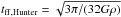 derived for gravitational collapse by Hunter (1962), where a constant envelope density ρ is assumed. However, the steep power-law density p = 1.4 in the envelope and the presence of COM emission towards the central source indicate that the early collapse phase described by Hunter (1962) is over and that a sizeable point mass has formed in the center that now dominates the gravitational field on the small scales considered.
Acknowledgments
We are grateful to an anonymous referee for useful comments that helped to strengthen the paper. The research leading to these results has received funding from the French Agence Nationale de la Recherche (ANR), under reference ANR-12-JS05-0005. The project has received further support from the European Research Council under the European Union’s Seventh Framework Programme (ERC Advanced Grant Agreement No. 291294 – ORISTARS). L.P. has received funding from the European Union Seventh Framework Programme (FP7/2007-2013) under grant agreement No. 267251. We would also like to thank Bilal Ladjelate for his help in estimating the internal luminosities of the target sources from Herschel data. Furthermore, the authors would like to thank Edith Fayolle, Stéphane Guilloteau, Lars Kristensen, Karin Öberg, and Magnus Persson for valuable discussions, comments, and suggestions.
References
- Aikawa, Y., Umebayashi, T., Nakano, T., & Miyama, S. M. 1997, ApJ, 486, L51 [NASA ADS] [CrossRef] [Google Scholar]
- Alonso-Albi, T., Fuente, A., Crimier, N., et al. 2010, A&A, 518, A52 [NASA ADS] [CrossRef] [EDP Sciences] [Google Scholar]
- Andre, P., Ward-Thompson, D., & Barsony, M. 2000, Protostars and Planets IV, 59 [Google Scholar]
- André, P., Ward-Thompson, D., & Barsony, M. 1993, ApJ, 406, 122 [NASA ADS] [CrossRef] [Google Scholar]
- André, P., Men’shchikov, A., Bontemps, S., et al. 2010, A&A, 518, L102 [NASA ADS] [CrossRef] [EDP Sciences] [Google Scholar]
- Asplund, M., Grevesse, N., Sauval, A. J., & Scott, P. 2009, ARA&A, 47, 481 [NASA ADS] [CrossRef] [Google Scholar]
- Belloche, A., & André, P. 2004, A&A, 419, L35 [NASA ADS] [CrossRef] [EDP Sciences] [Google Scholar]
- Bachiller, R., Andre, P., & Cabrit, S. 1991, A&A, 241, L43 [NASA ADS] [Google Scholar]
- Bachiller, R., & Pérez Gutiérrez, M. 1997, ApJ, 487, L93 [NASA ADS] [CrossRef] [Google Scholar]
- Bachiller, R., Martin-Pintado, J., Tafalla, M., Cernicharo, J., & Lazareff, B. 1990, A&A, 231, 174 [NASA ADS] [Google Scholar]
- Bachiller, R., Guilloteau, S., Dutrey, A., Planesas, P., & Martin-Pintado, J. 1995, A&A, 299, 857 [NASA ADS] [Google Scholar]
- Bachiller, R., Pérez Gutiérrez, M., Kumar, M. S. N., & Tafalla, M. 2001, A&A, 372, 899 [NASA ADS] [CrossRef] [EDP Sciences] [Google Scholar]
- Belloche, A., André, P., Despois, D., & Blinder, S. 2002, A&A, 393, 927 [Google Scholar]
- Belloche, A., Hennebelle, P., & André, P. 2006, A&A, 453, 145 [NASA ADS] [CrossRef] [EDP Sciences] [Google Scholar]
- Bergin, E. A., Langer, W. D., & Goldsmith, P. F. 1995, ApJ, 441, 222 [NASA ADS] [CrossRef] [Google Scholar]
- Bergin, E. A., Ciardi, D. R., Lada, C. J., Alves, J., & Lada, E. A. 2001, ApJ, 557, 209 [NASA ADS] [CrossRef] [Google Scholar]
- Bisschop, S. E., Fraser, H. J., Öberg, K. I., van Dishoeck, E. F., & Schlemmer, S. 2006, A&A, 449, 1297 [NASA ADS] [CrossRef] [EDP Sciences] [Google Scholar]
- Blake, G. A., Sandell, G., van Dishoeck, E. F., et al. 1995, ApJ, 441, 689 [Google Scholar]
- Bottinelli, S., Ceccarelli, C., Lefloch, B., et al. 2004, ApJ, 615, 354 [NASA ADS] [CrossRef] [Google Scholar]
- Bottinelli, S., Ceccarelli, C., Williams, J. P., & Lefloch, B. 2007, A&A, 463, 601 [NASA ADS] [CrossRef] [EDP Sciences] [Google Scholar]
- Bottinelli, S., Ceccarelli, C., Neri, R., & Williams, J. P. 2008, in IAU Symp., 251, eds. S. Kwok, & S. Sanford, 117 [Google Scholar]
- Bottinelli, S., Boogert, A. C. A., Bouwman, J., et al. 2010, ApJ, 718, 1100 [NASA ADS] [CrossRef] [Google Scholar]
- Bringa, E. M., & Johnson, R. E. 2004, ApJ, 603, 159 [NASA ADS] [CrossRef] [Google Scholar]
- Chapillon, E., Guilloteau, S., Dutrey, A., & Piétu, V. 2008, A&A, 488, 565 [NASA ADS] [CrossRef] [EDP Sciences] [Google Scholar]
- Chiar, J. E., Adamson, A. J., Kerr, T. H., & Whittet, D. C. B. 1994, ApJ, 426, 240 [NASA ADS] [CrossRef] [Google Scholar]
- Choi, M. 2001, ApJ, 553, 219 [NASA ADS] [CrossRef] [Google Scholar]
- Cleeves, L. I., Bergin, E. A., Alexander, C. M. O., et al. 2014, Science, 345, 1590 [NASA ADS] [CrossRef] [Google Scholar]
- Codella, C., Lefloch, B., Ceccarelli, C., et al. 2010, A&A, 518, L112 [NASA ADS] [CrossRef] [EDP Sciences] [Google Scholar]
- Codella, C., Maury, A. J., Gueth, F., et al. 2014, A&A, 563, L3 [NASA ADS] [CrossRef] [EDP Sciences] [Google Scholar]
- Codella, C., Fontani, F., Ceccarelli, C., et al. 2015, MNRAS, 449, L11 [NASA ADS] [CrossRef] [Google Scholar]
- Collings, M. P., Dever, J. W., Fraser, H. J., McCoustra, M. R. S., & Williams, D. A. 2003, ApJ, 583, 1058 [NASA ADS] [CrossRef] [Google Scholar]
- Collings, M. P., Anderson, M. A., Chen, R., et al. 2004, MNRAS, 354, 1133 [NASA ADS] [CrossRef] [Google Scholar]
- Coutens, A., Vastel, C., Cabrit, S., et al. 2013, A&A, 560, A39 [NASA ADS] [CrossRef] [EDP Sciences] [Google Scholar]
- Cuppen, H. M., van Dishoeck, E. F., Herbst, E., & Tielens, A. G. G. M. 2009, A&A, 508, 275 [NASA ADS] [CrossRef] [EDP Sciences] [Google Scholar]
- Curiel, S., Raymond, J. C., Moran, J. M., Rodriguez, L. F., & Canto, J. 1990, ApJ, 365, L85 [NASA ADS] [CrossRef] [Google Scholar]
- Daniel, F., Dubernet, M.-L., Meuwly, M., Cernicharo, J., & Pagani, L. 2005, MNRAS, 363, 1083 [NASA ADS] [CrossRef] [Google Scholar]
- Daranlot, J., Hincelin, U., Bergeat, A., et al. 2012, Proc. Nat. Acad. Sci., 109, 10233 [Google Scholar]
- Di Francesco, J., Myers, P. C., Wilner, D. J., Ohashi, N., & Mardones, D. 2001, ApJ, 562, 770 [NASA ADS] [CrossRef] [Google Scholar]
- Dunham, M. M., Crapsi, A., Evans, II, N. J., et al. 2008, ApJS, 179, 249 [NASA ADS] [CrossRef] [Google Scholar]
- Dunham, M. M., Arce, H. G., Allen, L. E., et al. 2013, AJ, 145, 94 [NASA ADS] [CrossRef] [Google Scholar]
- Dutrey, A., Guilloteau, S., & Simon, M. 2003, A&A, 402, 1003 [NASA ADS] [CrossRef] [EDP Sciences] [Google Scholar]
- Favre, C., Cleeves, L. I., Bergin, E. A., Qi, C., & Blake, G. A. 2013, ApJ, 776, L38 [NASA ADS] [CrossRef] [Google Scholar]
- Fayolle, E. C., Öberg, K. I., Cuppen, H. M., Visser, R., & Linnartz, H. 2011, A&A, 529, A74 [NASA ADS] [CrossRef] [EDP Sciences] [Google Scholar]
- Fayolle, E. C., Balfe, J., Loomis, R., et al. 2016, ApJ, 816, L28 [NASA ADS] [CrossRef] [Google Scholar]
- Fuente, A., Caselli, P., McCoey, C., et al. 2012, A&A, 540, A75 [NASA ADS] [CrossRef] [EDP Sciences] [Google Scholar]
- Garrod, R. T., & Herbst, E. 2006, A&A, 457, 927 [NASA ADS] [CrossRef] [EDP Sciences] [Google Scholar]
- Gueth, F., Guilloteau, S., & Bachiller, R. 1996, A&A, 307, 891 [NASA ADS] [Google Scholar]
- Hasegawa, T. I., Herbst, E., & Leung, C. M. 1992, ApJS, 82, 167 [NASA ADS] [CrossRef] [Google Scholar]
- Hincelin, U., Wakelam, V., Hersant, F., et al. 2011, A&A, 530, A61 [NASA ADS] [CrossRef] [EDP Sciences] [Google Scholar]
- Hirano, N., Ho, P. P. T., Liu, S.-Y., et al. 2010, ApJ, 717, 58 [NASA ADS] [CrossRef] [Google Scholar]
- Hirota, T., Bushimata, T., Choi, Y. K., et al. 2008, PASJ, 60, 37 [NASA ADS] [CrossRef] [Google Scholar]
- Hirota, T., Honma, M., Imai, H., et al. 2011, PASJ, 63, 1 [NASA ADS] [CrossRef] [Google Scholar]
- Hogerheijde, M. R., & van der Tak, F. F. S. 2000, A&A, 362, 697 [NASA ADS] [Google Scholar]
- Hogerheijde, M. R., van Dishoeck, E. F., Blake, G. A., & van Langevelde, H. J. 1998, ApJ, 502, 315 [NASA ADS] [CrossRef] [PubMed] [Google Scholar]
- Hunter, C. 1962, ApJ, 136, 594 [NASA ADS] [CrossRef] [Google Scholar]
- Jennings, R. E., Cameron, D. H. M., Cudlip, W., & Hirst, C. J. 1987, MNRAS, 226, 461 [NASA ADS] [CrossRef] [Google Scholar]
- Jørgensen, J. K. 2004, A&A, 424, 589 [NASA ADS] [CrossRef] [EDP Sciences] [Google Scholar]
- Jørgensen, J. K., & van Dishoeck, E. F. 2010a, ApJ, 725, L172 [NASA ADS] [CrossRef] [Google Scholar]
- Jørgensen, J. K., & van Dishoeck, E. F. 2010c, ApJ, 710, L72 [NASA ADS] [CrossRef] [Google Scholar]
- Jørgensen, J. K., Schöier, F. L., & van Dishoeck, E. F. 2002, A&A, 389, 908 [NASA ADS] [CrossRef] [EDP Sciences] [Google Scholar]
- Jørgensen, J. K., Harvey, P. M., Evans, II, N. J., et al. 2006, ApJ, 645, 1246 [NASA ADS] [CrossRef] [Google Scholar]
- Jørgensen, J. K., Bourke, T. L., Myers, P. C., et al. 2007, ApJ, 659, 479 [NASA ADS] [CrossRef] [Google Scholar]
- Jørgensen, J. K., Visser, R., Sakai, N., et al. 2013, ApJ, 779, L22 [NASA ADS] [CrossRef] [Google Scholar]
- Jørgensen, J. K., Visser, R., Williams, J. P., & Bergin, E. A. 2015, A&A, 579, A23 [NASA ADS] [CrossRef] [EDP Sciences] [Google Scholar]
- Karska, A., Herczeg, G. J., van Dishoeck, E. F., et al. 2013, A&A, 552, A141 [NASA ADS] [CrossRef] [EDP Sciences] [Google Scholar]
- Knee, L. B. G., & Sandell, G. 2000, A&A, 361, 671 [NASA ADS] [Google Scholar]
- Kristensen, L. E., van Dishoeck, E. F., Bergin, E. A., et al. 2012, A&A, 542, A8 [NASA ADS] [CrossRef] [EDP Sciences] [Google Scholar]
- Kun, M. 1998, ApJS, 115, 59 [NASA ADS] [CrossRef] [Google Scholar]
- Lauck, T., Karssemeijer, L., Shulenberger, K., et al. 2015, ApJ, 801, 118 [NASA ADS] [CrossRef] [Google Scholar]
- Liseau, R., Sandell, G., & Knee, L. B. G. 1988, A&A, 192, 153 [NASA ADS] [Google Scholar]
- Looney, L. W., Mundy, L. G., & Welch, W. J. 2000, ApJ, 529, 477 [NASA ADS] [CrossRef] [Google Scholar]
- Looney, L. W., Tobin, J. J., & Kwon, W. 2007, ApJ, 670, L131 [NASA ADS] [CrossRef] [Google Scholar]
- Maret, S., Ceccarelli, C., Caux, E., Tielens, A. G. G. M., & Castets, A. 2002, A&A, 395, 573 [NASA ADS] [CrossRef] [EDP Sciences] [Google Scholar]
- Maret, S., & Bergin, E. A. 2015, Astrophysics Source Code Library [record ascl:1507.010] [Google Scholar]
- Maret, S., Bergin, E. A., & Lada, C. J. 2006, Nature, 442, 425 [NASA ADS] [CrossRef] [PubMed] [Google Scholar]
- Maret, S., Belloche, A., Maury, A. J., et al. 2014, A&A, 563, L1 [NASA ADS] [CrossRef] [EDP Sciences] [Google Scholar]
- Martín-Doménech, R., Muñoz Caro, G. M., Bueno, J., & Goesmann, F. 2014, A&A, 564, A8 [NASA ADS] [CrossRef] [EDP Sciences] [Google Scholar]
- Mathews, G. S., Klaassen, P. D., Juhász, A., et al. 2013, A&A, 557, A132 [NASA ADS] [CrossRef] [EDP Sciences] [Google Scholar]
- Maury, A. J., Belloche, A., André, P., et al. 2014, A&A, 563, L2 [NASA ADS] [CrossRef] [EDP Sciences] [Google Scholar]
- Motte, F., & André, P. 2001, A&A, 365, 440 [NASA ADS] [CrossRef] [EDP Sciences] [Google Scholar]
- Noble, J. A., Congiu, E., Dulieu, F., & Fraser, H. J. 2012, MNRAS, 421, 768 [NASA ADS] [Google Scholar]
- Öberg, K. I., van Broekhuizen, F., Fraser, H. J., et al. 2005, ApJ, 621, L33 [NASA ADS] [CrossRef] [Google Scholar]
- Öberg, K. I., Boogert, A. C. A., Pontoppidan, K. M., et al. 2008, ApJ, 678, 1032 [NASA ADS] [CrossRef] [Google Scholar]
- Öberg, K. I., Linnartz, H., Visser, R., & van Dishoeck, E. F. 2009a, ApJ, 693, 1209 [NASA ADS] [CrossRef] [Google Scholar]
- Öberg, K. I., van Dishoeck, E. F., & Linnartz, H. 2009b, A&A, 496, 281 [NASA ADS] [CrossRef] [EDP Sciences] [Google Scholar]
- Penteado, E. M., Boogert, A. C. A., Pontoppidan, K. M., et al. 2015, MNRAS, 454, 531 [NASA ADS] [CrossRef] [Google Scholar]
- Persson, M. V., Jørgensen, J. K., & van Dishoeck, E. F. 2012, A&A, 541, A39 [NASA ADS] [CrossRef] [EDP Sciences] [Google Scholar]
- Podio, L., Lefloch, B., Ceccarelli, C., Codella, C., & Bachiller, R. 2014, A&A, 565, A64 [NASA ADS] [CrossRef] [EDP Sciences] [Google Scholar]
- Pontoppidan, K. M. 2006, A&A, 453, L47 [NASA ADS] [CrossRef] [EDP Sciences] [Google Scholar]
- Pontoppidan, K. M., Fraser, H. J., Dartois, E., et al. 2003, A&A, 408, 981 [NASA ADS] [CrossRef] [EDP Sciences] [Google Scholar]
- Pontoppidan, K. M., Boogert, A. C. A., Fraser, H. J., et al. 2008, ApJ, 678, 1005 [NASA ADS] [CrossRef] [Google Scholar]
- Prisinzano, L., Micela, G., Flaccomio, E., et al. 2008, ApJ, 677, 401 [NASA ADS] [CrossRef] [Google Scholar]
- Qi, C., D’Alessio, P., Öberg, K. I., et al. 2011, ApJ, 740, 84 [NASA ADS] [CrossRef] [Google Scholar]
- Qi, C., Öberg, K. I., Wilner, D. J., et al. 2013, Science, 341, 630 [NASA ADS] [CrossRef] [PubMed] [Google Scholar]
- Qi, C., Öberg, K. I., Andrews, S. M., et al. 2015, ApJ, 813, 128 [NASA ADS] [CrossRef] [Google Scholar]
- Rabli, D., & Flower, D. R. 2010, MNRAS, 406, 95 [NASA ADS] [CrossRef] [Google Scholar]
- Reboussin, L., Wakelam, V., Guilloteau, S., Hersant, F., & Dutrey, A. 2015, A&A, 579, A82 [NASA ADS] [CrossRef] [EDP Sciences] [Google Scholar]
- Ripple, F., Heyer, M. H., Gutermuth, R., Snell, R. L., & Brunt, C. M. 2013, MNRAS, 431, 1296 [NASA ADS] [CrossRef] [Google Scholar]
- Sadavoy, S. I., Di Francesco, J., André, P., et al. 2014, ApJ, 787, L18 [NASA ADS] [CrossRef] [Google Scholar]
- Sakai, N., Sakai, T., & Yamamoto, S. 2006, PASJ, 58, L15 [NASA ADS] [Google Scholar]
- Sakai, N., Ceccarelli, C., Bottinelli, S., Sakai, T., & Yamamoto, S. 2012, ApJ, 754, 70 [NASA ADS] [CrossRef] [Google Scholar]
- Sandell, G., Aspin, C., Duncan, W. D., Russell, A. P. G., & Robson, E. I. 1991, ApJ, 376, L17 [NASA ADS] [CrossRef] [Google Scholar]
- Sandford, S. A., & Allamandola, L. J. 1988, Icarus, 76, 201 [NASA ADS] [CrossRef] [Google Scholar]
- Sandford, S. A., & Allamandola, L. J. 1993, ApJ, 417, 815 [NASA ADS] [CrossRef] [PubMed] [Google Scholar]
- Santangelo, G., Codella, C., Cabrit, S., et al. 2015, A&A, 584, A126 [NASA ADS] [CrossRef] [EDP Sciences] [Google Scholar]
- Schöier, F. L., van der Tak, F. F. S., van Dishoeck, E. F., & Black, J. H. 2005, A&A, 432, 369 [NASA ADS] [CrossRef] [EDP Sciences] [Google Scholar]
- Scott, P. C., Asplund, M., Grevesse, N., & Sauval, A. J. 2006, A&A, 456, 675 [NASA ADS] [CrossRef] [EDP Sciences] [Google Scholar]
- Stäuber, P., Benz, A. O., Jørgensen, J. K., et al. 2007, A&A, 466, 977 [NASA ADS] [CrossRef] [EDP Sciences] [Google Scholar]
- Tafalla, M., Bachiller, R., Lefloch, B., et al. 2015, A&A, 573, L2 [NASA ADS] [CrossRef] [EDP Sciences] [Google Scholar]
- Taquet, V., López-Sepulcre, A., Ceccarelli, C., et al. 2015, ApJ, 804, 81 [NASA ADS] [CrossRef] [Google Scholar]
- Tobin, J. J., Looney, L. W., Mundy, L. G., Kwon, W., & Hamidouche, M. 2007, ApJ, 659, 1404 [NASA ADS] [CrossRef] [Google Scholar]
- Visser, R., Kristensen, L. E., Bruderer, S., et al. 2012, A&A, 537, A55 [NASA ADS] [CrossRef] [EDP Sciences] [Google Scholar]
- Visser, R., Bergin, E. A., & Jørgensen, J. K. 2015, A&A, 577, A102 [NASA ADS] [CrossRef] [EDP Sciences] [Google Scholar]
- Wakelam, V., & Herbst, E. 2008, ApJ, 680, 371 [NASA ADS] [CrossRef] [Google Scholar]
- Whittet, D. C. B., Shenoy, S. S., Bergin, E. A., et al. 2007, ApJ, 655, 332 [NASA ADS] [CrossRef] [Google Scholar]
- Whittet, D. C. B., Cook, A. M., Chiar, J. E., et al. 2009, ApJ, 695, 94 [NASA ADS] [CrossRef] [Google Scholar]
- Whittet, D. C. B., Cook, A. M., Herbst, E., Chiar, J. E., & Shenoy, S. S. 2011, ApJ, 742, 28 [NASA ADS] [CrossRef] [Google Scholar]
- Yang, B., Stancil, P. C., Balakrishnan, N., & Forrey, R. C. 2010, ApJ, 718, 1062 [NASA ADS] [CrossRef] [Google Scholar]
- Yıldız, U. A., van Dishoeck, E. F., Kristensen, L. E., et al. 2010, A&A, 521, L40 [NASA ADS] [CrossRef] [EDP Sciences] [Google Scholar]
- Yıldız, U. A., Kristensen, L. E., van Dishoeck, E. F., et al. 2012, A&A, 542, A86 [NASA ADS] [CrossRef] [EDP Sciences] [Google Scholar]
- Zhang, Q., Ho, P. T. P., & Wright, M. C. H. 2000, AJ, 119, 1345 [NASA ADS] [CrossRef] [Google Scholar]
Appendix A: The full sample of sources
Among the 16 sources that were observed in the CALYPSO programme, we chose the four sources that show a clear anti-correlation in their emission of C18O and N2H+, for our analysis. In the remaining sources, we detect C18O at a level of more than 3σ in all cases, and in six sources at a level of more than 9σ (L1527, IRAS2A, SVS-13A, L1448-2A, GF9-2, SERP-SMM4). In two cases, C18O is detected towards two positions (SVS13, AQU-MMS1, SERP-SMM4) at a level of more than 6σ. N2H+ is detected in all fields of a size of 10′′ around the main source at a level of more than 3σ. Three sources show only weak emission (<6σ: L1527, L1521F, AQU-MMS2), while the other sources show emission levels of 7−11σ.
In the sample, four different morphologies can be distinguished:
-
1.
One-sided anticorrelation, where the source appears located at the edge of an N2H+ filament, strong emission in C18O and adjacent peak in N2H+.
-
2.
No or weak emission of N2H+, or no or weak emission of C18O in our data.
-
3.
C18O and N2H+ are both detected towards the source without a clear anti-correlation, relatively weak emission in C18O, strong, relatively uniform emission in N2H+.
-
4.
Compact C18O emission towards the source, no N2H+ emission towards the source, large N2H+ ring around the source not adjacent to the C18O emission.
According to this scheme, the observed sources could be classified as follows:
-
1.
IRAS2A, L1448-2A, SVS-13A, GF9-2, SERP-S68N, SERP-SMM4, AQU-MMS1.
-
2.
L1527, L1521-F, AQU-MMS2.
-
3.
L1448-N, SVS13-B.
-
4.
IRAM04191.
We show four sources representing each of the different morphologies in Fig. A.1: IRAS2A representing class 1, L1527 representing class 2, L1448-N representing class 3, and IRAM04191 representing class 4. The different morphologies seem to suggest that if (a) the source emits strongly in C18O and if (b) the source is fully embedded in an N2H+-rich environment, an anti-correlation is always seen. If the source emits strongly in C18O and sits at the edge of an N2H+ filament, the anti-correlation appears only one-sided (Case 1). On the other hand, if there is either no C18O or no N2H+, obviously no anti-correlation is observed at all (Case 2). There also seems
to be cases where C18O does not appear abundant enough to significantly destroy N2H+ towards the source (Case 3). As already mentioned in Sect. 4.3, IRAM04191 stands out in the sense that the large ring emission of N2H+ might hint at a past accretion burst (Case 4).
 |
Fig. A.1 N2H+ and C18O integrated intensity maps for IRAS2A (top left), L1527 (top right), L1448-N (bottom left), and IRAM04191 (bottom right) as prototypical sources for the four morphology classes we find in the full sample of sources. Color background: N2H+ (1–0) emission integrated over all seven hyperfine components. The noise in these maps is σ = (0.043, 0.012, 0.033, 0.032) Jy beam-1 km s-1 for IRAS2A, L1527, L1448-N, and IRAM04191, respectively. The wedges show the N2H+ intensity scale in Jy beam-1 km s-1. Note that while for the first three sources the FOV is 20′′× 20′′, it is 40′′× 40′′ for IRAM04191 to show the full ring-like morphology. Contours show integrated emission of C18O (2–1) in steps of 3σ, starting at 3σ up to 60σ, with σ = (0.037, 0.022, 0.038, 0.018) Jy beam-1 km s-1 for IRAS2A, L1527, L1448-N, and IRAM04191, respectively. The C18O emission was integrated over ±3 km s-1 around the systemic velocity of each source. The inlay in the upper right corners of the top left panel shows the methanol emission towards IRAS2A as color background and contours in steps of 3σ, starting at 3σ up to 60σ inside the central 2′′. The filled ellipses in the lower left corner of the panels indicate the synthesized beam sizes of the N2H+ observations at 3 mm. The dashed white lines illustrate the small-scale outflow directions (See Codella et al. 2014; Hogerheijde et al. 1998; Podio et al. in prep.; Belloche et al. 2002). |
Appendix B: CO and CH3OH uv data
In Sect. 3.3, we followed the standard procedure of using circular and elliptical Gaussian uv-fits in order to measure the size of the source emission in C18O and CH3OH. Figures B.1 and B.2 show plots of the uv data, obtained by radially averaging the data that was used for the fits listed in Tables 3 and 4. While the radial average hides all the complex spatial morphological structure that is visible in the maps shown in Fig. 1, it may still give an impression of the quality of the data. For comparison, the results of the elliptical and circular Gaussian fits are shown as well, which may hint at the strength of radial variations mirrored in the eccentricity of the elliptical fits.
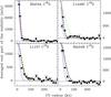 |
Fig. B.1 C18O uv plots for IRAS4A (top left), L1448C (top right), L1157 (bottom left) and IRAS4B (bottom right). The data is integrated over ±3 km s-1 around the line center and radially averaged in bins of 20 m with task uv_circle in MAPPING. Red lines show the results of the circular Gaussian fits to the un-averaged uv data, while the blue and green lines show the results of the elliptical Gaussian fits to the un-averaged uv data along the major and minor axes, respectively. Black dashed lines show the result of the elliptical Gaussian fits with fixed PA along the outflow. The parameters of the fits are listed in Table 3. |
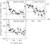 |
Fig. B.2 Same as Fig. B.1, but for CH3OH in IRAS4A (top left), L1448C (top right), and IRAS4B (bottom left). The data is radially averaged in bins of 50 m with task uv_circle in MAPPING. The parameters of the fits are listed in Table 4. |
Appendix C: Model parameter dependences
Figure C.1 illustrates the dependence of the chemical model on the most important free parameters. As discussed in Sect. 4.1, the computed C18O abundance is independent of the assumed chemical age, while CH3OH and N2H+ get destroyed with time (see top left panel). Therefore, our observations do not constrain the
initial fractional abundances for these two latter species, because the inference from the final abundances fed into Ratran to the initial abundances of CH3OH and N2H+ relies on the unknown chemical age. The top right panel of Fig. C.1 shows how the CO emission size varies with the assumed CO-binding energy. This plot also demonstrates that for the anti-correlation between CO and N2H+ to be established, the N2 binding energy has to be smaller than the binding energy of CO. The bottom left panel shows that all C18O that is initially put into ices will be found in the gas phase inside of the snow line, such that the resulting CO peak intensity can directly be fine-tuned by varying the initial fractional CO abundance. Finally, as already discussed in Sect. 4.1, the bottom right panel demonstrates that both the CO and CH3OH abundance profiles do not depend on the assumed initial water abundance.
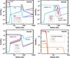 |
Fig. C.1 Dependences of the chemical model on various free parameters. Top left: the fractional abundances of CH3OH, C18O, and N2H+ are shown for four different chemical ages. Same colors identify abundance curves at the same chemical time for chemical ages as indicated in the legend. Top right: the fractional abundances of C18O (dashed lines) and N2H+ (full lines) are displayed for different values of the CO binding energy. Same colors identify abundance curves computed with the same CO binding energy as indicated in the legend. Bottom left: the fractional abundances of C18O (dashed lines) and N2H+ (full lines) are displayed for different values of the initial fractional CO abundance. Same colors identify abundance curves computed with the same CO initial abundance as indicated in the legend. Bottom right: the fractional abundances of H2O, CH3OH, and C18O are shown for four different values of the initial fractional H2O abundance. Same colors identify abundance curves computed with the same H2O initial abundance as indicated in the legend. |
Appendix D: Initial abundances for Astrochem
Table D.1 lists the initial fractional abundances relative to H2 used in the chemical computations with Astrochem. For the metals, the low-metal case, as described in Wakelam & Herbst (2008), was adopted. The molecules were initially put into ices, because the sublimation timescale is much smaller than the desorption timescale inside of the snow line (see Fig. 7) such that the molecules quickly return into the gas phase in that region.
Initial fractional abundances used in Astrochem, relative to H2.
All Tables
Synthesized beam sizes and rms noise per channel in the final datacubes for the observed lines and sources.
Results of elliptical and circular Gaussian fits in the uv plane to the C18O emission integrated over ±3 km s-1, performed with task uv_fit in MAPPING.
Results of elliptical and circular Gaussian fits in the uv plane to the CH3OH emission integrated over ±3 km s-1, performed with task uv_fit in MAPPING.
All Figures
|
Fig. 1 Anticorrelation between N2H+ and C18O. Color background: N2H+ (1–0) emission integrated over all seven hyperfine components. The noise in these maps is σ = (0.030, 0.027, 0.025, 0.029) Jy beam-1 km s-1 for IRAS4A, L1448C, L1157, and IRAS4B, respectively. The wedges show the N2H+ intensity scale in Jy beam-1 km s-1. For the two lower panels the scaling is the same. Contours show emission of C18O (2–1) in steps of 6σ (IRAS4A) or 3σ (L1448C, L1157, and IRAS4B), starting at 3σ, with σ = (0.044, 0.029, 0.031, 0.033) Jy beam-1 km s-1 for IRAS4A, L1448C, L1157, and IRAS4B, respectively. The inlays in the upper right corners show the methanol emission as color background and contours in steps of 3σ, starting at 3σ inside the central 2′′, with σ = (0.028, 0.019, 0.027) Jy beam-1 km s-1 for IRAS4A, L1448C, and IRAS4B. In L1157, the methanol line has not been detected at a 3σ level. The filled ellipses in the lower left corner of the panels indicate the synthesized beam sizes of the N2H+ observations at 3 mm. The dashed white lines illustrate the small-scale outflow directions (see Table 3 and Sect. 3.1), and the white crosses show the positions of the sources as listed in Table 1. |
| In the text | |
|
Fig. 2 Top row: comparison of the observations (contours) with the synthetic maps (color background) produced by the best fit model for IRAS4B with Eb(CO) = 1200 K and Eb(N2) = 1000 K. Top left: C18O (2−1), center: N2H+ (1–0), right: CH3OH (51−42), integration intervals are the same as in Fig. 1, while the contour spacing is in steps of 3σ, starting at 3σ. The white dashed lines show the outflow direction, while the dotted lines show the direction of the intensity cuts. The scaling of the maps can be understood in comparison with the cuts in the bottom row. Bottom row: cuts perpendicular to the outflow direction (PA = 0°) for C18O, N2H+, and CH3OH (left to right). Gray lines show the data, red lines the model. The blue bars in the top right corners of the bottom panels show the HPBW along the cut. |
| In the text | |
|
Fig. 3 Fractional chemical abundances, relative to H2, of C18O (red lines), N2H+ (blue lines), and CH3OH (green lines), computed by Astrochem for the envelope structures of IRAS4A (top left), L1448C (top right), L1157 (bottom left), and IRAS4B (bottom right). The light gray dotted lines show the HWHM of the modeled emission, the dark gray dotted lines the HWHM of the observed emission in C18O (see Table 3), while the light blue dashed line shows the location of the CO snow line in the model (see Table 5). The figure also indicates the dust temperature values at the respective radii. In IRAS4B, the observed and modeled HWHM are the same. |
| In the text | |
|
Fig. 4 Same as Fig. 2, but for IRAS4A. The cuts are performed at a PA of 90° perpendicular to the outflow direction (PA = 0°). |
| In the text | |
|
Fig. 5 Same as Fig. 2, but for L1448C. The cuts are performed at a PA of 70° perpendicular to the outflow direction (PA = 160°). |
| In the text | |
|
Fig. 6 Same as Fig. 2, but without methanol, for L1157. The cuts are performed at a PA of 71°, perpendicular to the outflow direction (PA = 161°). |
| In the text | |
|
Fig. 7 CO ice depletion timescale (dark blue line) and thermal desorption timescales for binding energies of 855 K (orange line) and 1200 K (red line) as a function of the dust temperature for the density profiles of IRAS4B. The light blue line shows the free-fall time for an enclosed mass of 0.5 M⊙. The points of intersection at ~17 K and ~24 K indicate the locations of the CO snow line for the two different values of the binding energy. The gray area shows the range of depletion timescales if the dust density is varied by a factor of ten. For a binding energy of 855 K, the variation of the density translates into a variation of the snow line location at ~16 K or ~17 K, while for a binding energy of 1200 K, the modified snow line locations would be at ~23 K or ~25 K. |
| In the text | |
|
Fig. A.1 N2H+ and C18O integrated intensity maps for IRAS2A (top left), L1527 (top right), L1448-N (bottom left), and IRAM04191 (bottom right) as prototypical sources for the four morphology classes we find in the full sample of sources. Color background: N2H+ (1–0) emission integrated over all seven hyperfine components. The noise in these maps is σ = (0.043, 0.012, 0.033, 0.032) Jy beam-1 km s-1 for IRAS2A, L1527, L1448-N, and IRAM04191, respectively. The wedges show the N2H+ intensity scale in Jy beam-1 km s-1. Note that while for the first three sources the FOV is 20′′× 20′′, it is 40′′× 40′′ for IRAM04191 to show the full ring-like morphology. Contours show integrated emission of C18O (2–1) in steps of 3σ, starting at 3σ up to 60σ, with σ = (0.037, 0.022, 0.038, 0.018) Jy beam-1 km s-1 for IRAS2A, L1527, L1448-N, and IRAM04191, respectively. The C18O emission was integrated over ±3 km s-1 around the systemic velocity of each source. The inlay in the upper right corners of the top left panel shows the methanol emission towards IRAS2A as color background and contours in steps of 3σ, starting at 3σ up to 60σ inside the central 2′′. The filled ellipses in the lower left corner of the panels indicate the synthesized beam sizes of the N2H+ observations at 3 mm. The dashed white lines illustrate the small-scale outflow directions (See Codella et al. 2014; Hogerheijde et al. 1998; Podio et al. in prep.; Belloche et al. 2002). |
| In the text | |
|
Fig. B.1 C18O uv plots for IRAS4A (top left), L1448C (top right), L1157 (bottom left) and IRAS4B (bottom right). The data is integrated over ±3 km s-1 around the line center and radially averaged in bins of 20 m with task uv_circle in MAPPING. Red lines show the results of the circular Gaussian fits to the un-averaged uv data, while the blue and green lines show the results of the elliptical Gaussian fits to the un-averaged uv data along the major and minor axes, respectively. Black dashed lines show the result of the elliptical Gaussian fits with fixed PA along the outflow. The parameters of the fits are listed in Table 3. |
| In the text | |
|
Fig. B.2 Same as Fig. B.1, but for CH3OH in IRAS4A (top left), L1448C (top right), and IRAS4B (bottom left). The data is radially averaged in bins of 50 m with task uv_circle in MAPPING. The parameters of the fits are listed in Table 4. |
| In the text | |
|
Fig. C.1 Dependences of the chemical model on various free parameters. Top left: the fractional abundances of CH3OH, C18O, and N2H+ are shown for four different chemical ages. Same colors identify abundance curves at the same chemical time for chemical ages as indicated in the legend. Top right: the fractional abundances of C18O (dashed lines) and N2H+ (full lines) are displayed for different values of the CO binding energy. Same colors identify abundance curves computed with the same CO binding energy as indicated in the legend. Bottom left: the fractional abundances of C18O (dashed lines) and N2H+ (full lines) are displayed for different values of the initial fractional CO abundance. Same colors identify abundance curves computed with the same CO initial abundance as indicated in the legend. Bottom right: the fractional abundances of H2O, CH3OH, and C18O are shown for four different values of the initial fractional H2O abundance. Same colors identify abundance curves computed with the same H2O initial abundance as indicated in the legend. |
| In the text | |
Current usage metrics show cumulative count of Article Views (full-text article views including HTML views, PDF and ePub downloads, according to the available data) and Abstracts Views on Vision4Press platform.
Data correspond to usage on the plateform after 2015. The current usage metrics is available 48-96 hours after online publication and is updated daily on week days.
Initial download of the metrics may take a while.