| Issue |
A&A
Volume 591, July 2016
|
|
|---|---|---|
| Article Number | A65 | |
| Number of page(s) | 9 | |
| Section | Stellar structure and evolution | |
| DOI | https://doi.org/10.1051/0004-6361/201527193 | |
| Published online | 13 June 2016 | |
Suzaku observations of the 2013 outburst of KS 1947+300
1 Dr. Karl-Remeis-Sternwarte and Erlangen Centre for Astroparticle Physics, Sternwartstr. 7, 96049 Bamberg, Germany
2 Department of Physics, University of Maryland Baltimore County, Baltimore, MD 21250, USA
3 CRESST and NASA Goddard Space Flight Center, Astrophysics Science Division, Code 661, Greenbelt, MD 20771, USA
4 Cahill Center for Astronomy and Astrophysics, California Institute of Technology, Pasadena, CA 91125, USA
5 Center for Astrophysics and Space Sciences, University of California, San Diego, 9500 Gilman Dr., La Jolla, CA 920093-0424, USA
6 Kavli Institute for Astrophysics and Space Research, Massachusetts Institute of Technology, Cambridge, MA 02139, USA
7 Science Operations Division, Science Operations Department of ESA, ESAC, 28692 Villanueva de la Cañada, Madrid, Spain
Received: 14 August 2015
Accepted: 1 March 2016
We report on the timing and spectral analysis of two Suzaku observations with different flux levels of the high-mass X-ray binary KS 1947+300 during its 2013 outburst. In agreement with simultaneous NuSTAR observations, the continuum is well described by an absorbed power law with a cutoff and an additional blackbody component. In addition, we find fluorescent emission from neutral, He-like, and even H-like iron. We determine a pulse period of ~18.8 s with the source showing a spin-up between the two observations. Both Suzaku observations show very similar behavior of the pulse profile, which is strongly energy dependent. This profile has an evolution from a profile with one peak at low energies to a profile with two peaks of different widths toward higher energies seen in both the Suzaku and NuSTAR data. Such an evolution to a more complex profile at higher energies is rarely seen in X-ray pulsars, most cases show the opposite behavior. Pulse phase-resolved spectral analysis shows a variation in the absorbing column density, NH, over pulse phase. Spectra taken during the pulse profile minima are intrinsically softer compared to the pulse phase-averaged spectrum.
Key words: pulsars: individual: KS 1947+300 / X-rays: binaries / accretion, accretion disks
© ESO, 2016
1. Introduction
KS 1947+300 is an accretion powered X-ray pulsar in the constellation Cygnus. It was discovered on 1989 June 8 by the TTM instrument on the Kvant module of the Mir space station at a flux level of 70 ± 10 mCrab in the 2–27 keV band (Borozdin et al. 1990). The energy spectrum of this pulsar can be described by an absorbed power law of photon index 1.72 ± 0.31 and an equivalent hydrogen column density of (3.4 ± 3.0) × 1022 cm-2.
In 1994, this source was rediscovered as GRO J1948+32 by the Burst and Transient Science Experiment on the Compton Gamma-Ray Observatory. It was identified as an X-ray pulsar with a pulse period of ~18.7 s. This observation also allowed for a first estimate of the orbital parameters (Chakrabarty et al. 1995). Further RXTE observations of an outburst in 2000–2001 proved that KS 1947+300 and GRO J1948+32 are the same object (Levine & Corbet 2000; Swank & Morgan 2000). Its orbit was found to have an eccentricity e = 0.033 ± 0.013, an orbital period Porb = 40.415 ± 0.010 d, and a semimajor axis of asini = 137.4 lt-s (Galloway et al. 2004). The optical companion was identified as a B0Ve star (Negueruela et al. 2003).
Naik et al. (2006) presented a broadband spectral analysis using three BeppoSAX observations of the 2000 November to 2001 June outburst. Their spectral model consisted of a Comptonized continuum, a blackbody component with a temperature of ~0.6 keV, and an iron emission line at 6.7 keV. Tsygankov & Lutovinov (2005) reported on INTEGRAL observations taken from 2002 December to 2004 April and presented studies on the evolution of the pulse profile and period. These authors found a proportionality of the pulsation frequency and flux near the peak of the outburst, although at low significance, and they also observed a flux dependence of the pulse profile shape.
In this paper we report on the analysis of two Suzaku observations from 2013 October and 2013 November taken during the first outburst of this source since 2004. These observations were quasi-simultaneous with Nuclear Spectroscopic Telescope Array (NuSTAR) observations in which Fürst et al. (2014) present evidence for the presence of a Cyclotron Resonant Scattering Feature (CRSF or cyclotron line) at 12.2 keV. The detection of CRSFs allows us to directly infer the magnetic field strength in the emission region, which is a fundamental parameter of the neutron star (see, e.g., Harding & Lai 2006, for a review). Suzaku provides high sensitivity at low energies and therefore allows us to study the soft component of the broadband continuum, which is not available from NuSTAR alone, including the absorption and iron fluorescence emission.
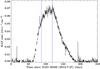 |
Fig. 1 Swift/BAT daily light curve in the 15–50 keV band of the outburst in 2013. The blue vertical lines indicate the times covered by Suzaku observations. |
The paper is organized as follows: Sect. 2 gives an overview of the data acquisition and reduction. In Sect. 3, we investigate the shape, energy dependence, and evolution of the pulse profiles. Phase-averaged and phase-resolved spectral analyses are presented in Sects. 4 and 5, respectively. In Sect. 6, we summarize and discuss our results.
2. Observation and data reduction
2.1. Suzaku
Suzaku is a joint mission of JAXA and NASA. It carries two main detectors: the X-ray Imaging Spectrometer (XIS; Takahashi et al. 2007) and the Hard X-ray Detector (HXD; Koyama et al. 2007). The XIS consists of four individual but identical Type-I Wolter telescopes (XRT), focusing the X-rays on CCD cameras. The XIS1 camera is back-illuminated, providing higher sensitivity at lower energies than the other front-illuminated configurations with a maximum energy range of 0.2–12 keV for all XIS (Takahashi et al. 2007). In 2006, XIS2 was damaged by a micro-meteorite impact and became unusable. The HXD consists of a collimated PIN silicon diode array (PIN) and a GSO/BGO phoswitch counter (GSO), covering a total energy range of 10–600 keV (Koyama et al. 2007).
Suzaku observed the 2013 outburst of KS 1947+300 twice, approximately one month apart and partially coinciding with NuSTAR observations. The observation log is summarized in Table 1. Figure 1 shows the Swift/BAT light curve of KS 1947+300 (Krimm et al. 2013) with times of the Suzaku observations marked. During both observations, XIS was operated in 1/4 window mode and clocking modes were set to “normal” and “burst” for the first (Obs. I) and second observations (Obs. II), respectively.
We used the software package HEAsoft (v. 6.15.1) for all Suzaku reprocessing and extraction. Standard screening criteria and calibration were applied by running aepipeline on both data sets. All event times were transferred to the solar barycenter using aebarycen. We used Suzaku CALDB v20110630 for XRT, v20110913 for HXD, and v20130916 and v20131231 for the first and second XIS data set, respectively.
Most likely because of incorrect attitude determination, the conversion of XIS detector to sky coordinates yields incorrect values for the first observation. As a result, the sky image cannot be properly reconstructed and shows two distinct sources. We therefore performed all data extractions for this observation in detector coordinates and regions are given in units of pixels. This method does not faciliate an additional attitude correction with the FTOOL aeattcor2 (see Uchiyama et al. 2008, for details). As the variation of the effective area with off-axis angle is small, the systematic error introduced by this choice is small and does not affect our analysis.
For the second observation, aeattcor2 was used for further improvement of the attitude of the spacecraft. We used annular extraction regions for XIS with outer radii of 125 pixels (Obs. I) and  (Obs. II). Inner radii were set individually to exclude all regions with pile-up fractions larger than 4% (65–72 pixels for Obs. I and 35″ for Obs. II), which were estimated using pileest. The XIS light curves were extracted with a 2 s time resolution, which is the highest possible resolution for the selected operating modes.
We applied the PIN response for calibration epoch 11 for the XIS nominal pointing position. We used the PIN “tuned” background (v2.2) as the non-X-ray background model (Fukazawa et al. 2009) for all analyses and also took the cosmic X-ray background into account (Boldt 1987). We applied the GSO correction ARF, provided by the Suzaku HXD team to improve the calibration of this instrument (see Yamada et al. 2011, for details) to both observations. The PIN has a nominal time resolution of 61 μs. Because the good time intervals corresponding to the phase bins are too short for an individual correction, the overall loss of artificially triggered “pseudo” events was used to estimate the dead time for the pulse profiles.
We extracted light curves and spectra for all available Suzaku instruments using xselect for the XIS, and the Suzaku specific FTOOLs hxdpinxbpi/hxdpinxblc and hxdgsoxbpi/hxdgsoxblc for the extraction of the PIN and the GSO data, respectively.
In order to avoid well-known uncertainties in the effective area and response matrix determination, we considered only the energy range of 1–10 keV for XIS0 and XIS3 and 1–8 keV for XIS1 for the spectral analysis. The energy ranges of 1.72–1.88 keV and 2.19–2.37 keV were excluded for all XIS because of known Au and Si calibration features (Nowak et al. 2011). For PIN and GSO, we used the energy ranges of 15–70 keV and 70–90 keV, respectively. We used the Interactive Spectral Interpretation System (ISIS v1.6.2; Houck & Denicola 2000). Uncertainties are given at the 90% confidence level (CL) for one parameter of interest unless otherwise noted.
Observation log for the two Suzaku and NuSTAR observations.
2.2. NuSTAR
As mentioned above, simultaneous to our Suzaku observations there were also two NuSTAR observations which were that previously published by Fürst et al. (2014). We use these data to better illustrate the interpretation of the pulse profile evolution with energy than what is possible with Suzaku alone (Sect. 3). We extracted the NuSTAR data from ObsID 80002015004 using the standard pipeline nupipline v. 1.4.1 as distributed with HEAsoft v. 6.16 and CALDB v. 20150316. We used the same extraction regions as Fürst et al. (2014), i.e., radii of 130″ and 105″, for the source and background, respectively. Light curves were extracted with 0.5 s time resolution. This time resolution is nominally faster than the available dead time calculation, which is only available on a 1 s basis. However, KS 1947+300 is varying smoothly on these timescales so that averaging over 1 s bins for the dead time does not introduce significant errors in the count rate estimate. The extracted light curves were barycentered to the solar system.
3. Timing analysis
The light curves of both Suzaku observations show no sign of flaring or significant variability and, therefore indicate that time resolved spectroscopy is not necessary. The absolute variability amplitude in the light curve is higher in Obs. II, but the relative variability is similar. We note that the hardness ratio was roughly the same in both observations (see Fig. 2).
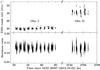 |
Fig. 2 Light curve and hardness ratio of XIS3 of both observations with 128 s time bins. The light curve covers the energy range 1–10 keV. The hardness ratio is defined as the ratio of the count rate in the 7–10 keV band to the count rate in the 1–4 keV band. |
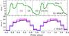 |
Fig. 3 Background-subtracted pulse profiles of Obs. I. The upper panel shows the PIN profiles with the phase intervals chosen for phase-resolved spectral analysis. The lower panel shows the XIS0 (blue), XIS1 (red), XIS3 (magenta) profiles. The pulse profiles are very similar to those of Obs. II. All profiles are shown twice for clarity. |
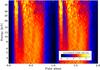 |
Fig. 4 Color-coded map of the count rate distribution of the NuSTAR observation as a function of energy and pulse phase. Each row represents a normalized pulse profile at the respective energy and each column, technically, indicates a phase-resolved spectrum. All profiles are shown twice for clarity. |
Pulse periods were determined for both observations using the epoch folding technique (Leahy et al. 1983): Pulse profiles are calculated for a series of test periods, assuming that for the correct period the corresponding pulse profile shows the most distinct shape, whereas for any other test period the averaging over a large number of pulses leads to a smoothing of the resulting profile. We did not use GSO for the pulse period determination because of its low statistics. Uncertainties of the pulse periods were estimated by simulating light curves based on the previously determined pulse profiles with additional Poisson noise. Epoch folding was then applied to a large number (in our case 10 000) of simulated light curves. The standard deviation of the pulse periods obtained with this simulation was taken as uncertainty of the pulse period of the data. All Suzaku detectors are in very good agreement with each other, but we quote the value of PIN, since it has the highest time resolution. The measured pulse periods are 18.80876(7) s and 18.78896(7) s for Obs. I and Obs. II, respectively. Thus, the source showed spin-up between the observations as was also observed by Fürst et al. (2014). We note, however, that the light curves have not been corrected for binary motion because of an accumulation of the uncertainties of the orbital parameters since 2000/2001. We estimated the possible impact of binary motion on the determined spin-up by correcting the photon arrival times using the orbital parameters of Galloway et al. (2004). We found that, even assuming that the phase information is lost completely, binary motion can only account for ~30% of the observed pulse period change. We therefore conclude that the observed spin-up is at least partly caused by the transfer of angular momentum to the neutron star.
The shape and evolution of the pulse profile look very similar for both observations and are therefore shown only for the first observation in Fig. 3. The pulse profiles in the XIS and PIN are significantly different from each other. The soft pulse profile consists of only one broad peak, whereas the hard profile is more complex and consists of a narrow peak and a broad peak at higher energies. This characteristic evolution of the pulse profile with energy has already been observed during previous outbursts (see, e.g., Tsygankov & Lutovinov 2005; Naik et al. 2006).
Using the Suzaku data alone, however, the analysis of evolution of the pulse profile at low energies is limited by the 2 s time resolution of the XIS. We took advantage of the excellent time resolution of NuSTAR to investigate the pulse profile evolution also at soft energies in more detail. We determined the local pulse period of the NuSTAR data to be 18.78779 s. We extracted light curves in 40 energy bins between 3–50 keV and folded them on this pulse period using 60 phase bins. Figure 4 shows the resulting count rate distribution of NuSTAR as a function of energy and pulse phase. To account for the high-energy rollover of the spectrum of the pulsar, all pulse profiles were normalized to their mean count rate and are given in units of their standard deviation. The pulse map shows that the secondary peak starts to form at ~6 keV and is of comparable strength to the main peak above ~15 keV. Interestingly, we do not find any significant phase shifts around the cyclotron line energy as predicted by theory (Schönherr et al. 2014) and as observed in 4U 0115+634 by Ferrigno et al. (2011).
4. Phase-averaged spectroscopy
We now turn to a description of the X-ray spectrum of the source in both observations. For the first observation, the XIS spectra were jointly rebinned to a minimum signal-to-noise ratio (S/N) of 80, except for the energy range of 6–7 keV, which was rebinned to a minimum S/N of 65 to ensure higher resolution in the iron line region. The intrinsic energy resolution of XIS, which is around 190 eV FWHM at ~6 keV (Ozawa et al. 2009), is oversampled by a factor of 4–5 in the iron line region. The PIN spectrum was rebinned to a minimum S/N of 25 and for GSO a channel binning factor of three was applied. For the second observation we chose a minimum S/N of 70 for XIS (50 for 6–7 keV) to account for the shorter exposure time, but rebinned PIN and GSO with the requirements of the first observation.
Figure 5 shows the phase-averaged spectrum with the best-fit model for the second observation and the best-fit parameters for both observations are given in Table 2.
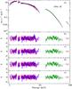 |
Fig. 5 a) Phase-averaged spectrum of Obs. II with best-fit model: XIS0 (blue), XIS1 (red), XIS3 (magenta), PIN (green) and GSO (brown). b) Residuals of continuum model without CRSF and Fe lines. c) Residuals of continuum model with narrow Kα and Kβ lines of neutral iron only and CRSF. d) Residuals of continuum model with both neutral and He-like Fe lines but without CRSF. e) Residuals of best-fit model including CRSF and Fe-lines. |
The best-fitting continuum model is an absorbed power law with an exponential cutoff of the form  (1)as used in ISIS/XSPEC with the photon index Γ and the folding energy Efold. An additional blackbody component with temperature kTBB was required to describe the spectrum below ~10 keV. Following Fürst et al. (2014), we used an updated version of the absorption model tbabs1, called tbnew with abundances and cross sections set according to Wilms et al. (2000) and Verner et al. (1996), respectively.
Tsujimoto et al. (2011) systematically investigated the cross-calibration of the individual XIS and reported that spectra observed with XIS1 tend to be slightly softer compared to XIS0 and XIS3. We therefore fitted the photon index of the back-illuminated XIS1 separately from the other XIS and HXD. The normalization and folding energy were required to be the same for all detectors during the fit. We confirm the result of Tsujimoto et al. (2011) that the photon index obtained from XIS1 is slightly higher compared to the other XIS and HXD, which agree with each other to within the confidence levels. As a result of the lower S/N of the phase-resolved spectra, this deviation of XIS1 and the other XIS can be ignored in the phase-resolved analysis.
Best-fit parameters and statistics for the phase-averaged spectra.
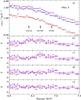 |
Fig. 6 Close-up plot of the iron line region for Obs. I. Panel a): XIS0 (blue), XIS1 (red), and XIS3 (magenta) data with the best-fitting model (black). Panel b): residuals for the continuum model only, i.e., without any emission lines. Panel c): residuals for the continuum model with the Kα line of neutral iron and panel d): residuals for the continuum model with both, neutral and He-like, Kα lines. Panel e): residuals for the continuum model with lines from neutral, He-like, and H-like iron included. All panels show the best fit for the respective model. |
Figure 6 shows the Fe line region of the spectrum for Obs. I and residuals for including different model components. For both observations, the Fe Kα and Kβ lines were modeled by two Gaussian emission lines. Furthermore, we fixed all line widths to 10-6 keV, assuming that line broadening is only due to the detector response. The Fe Kβ line is not significantly detected, i.e., adding it does not significantly improve the fit quality. However, if the line is due to fluorescence, then Fe Kβ emission has to be present at a known flux level and energy. We therefore included such a line at 0.65 keV higher than the Fe Kα line energy with a flux of 13% of the Kα line to the model (Palmeri et al. 2003). This did not introduce further fit parameters. Adding the Kα and Kβ line of neutral iron to our final continuum model reduced the χ2/ d.o.f from 1178.11/718 to 1016.06/716 for Obs I. and from 878.14/565 to 790.95/563 for Obs. II. It was furthermore necessary to add a third emission line at ~6.7 keV, the Kα line energy of He-like iron. Including this component again led to an improvement of χ2/ d.o.f to 906.22/714 for Obs. I and 741.03/561 for Obs. II. For the first observation, a fourth narrow emission line at ~6.9 keV, the Kα line energy of H-like iron, was also required, reducing the χ2/ d.o.f further to 893.53/712. This feature was not significantly detected in the second observation, possibly because of the lower exposure. The upper limit for the flux of this feature, however, is consistent with that measured during the first observation. We determined the significance of the H-like iron line with a Monte-Carlo approach (see, e.g., Protassov et al. 2002) and obtained a significance of 99.993% with 105 trials. For all other iron lines we found a significance of greater than 99.999%. Including a systematic uncertainty of 1.3% slightly reduces the detection significance of the H-like iron line to 99.978%. The other lines are not affected.
As mentioned above, Fürst et al. (2014) discovered a cyclotron line at 12.2 keV in the NuSTAR data. Unfortunately, this is exactly in the gap between the XIS and the HXD spectra. Since the line is rather wide, however, it can in principle still influence the Suzaku analysis. We therefore applied the continuum model both with and without the cyclotron line, describing the line by a Gaussian optical depth profile 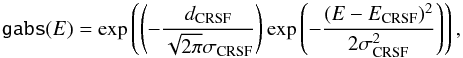 (2)with the line energy ECRSF, width σCRSF, and depth dCRSF.
As the Suzaku instruments do not cover the cyclotron line centroid energy, not all three parameters can be constrained simultaneously. We fixed the line energy and width to the values from Fürst et al. (2014) and only fitted the line strength. Fits that include the CRSF describe the data better, especially for Obs. II. In fact, Fürst et al. (2014) found the CRSF to be most prominent in the NuSTAR observation, which overlaps with the second Suzaku observation. Ignoring the CRSF leads to negative residuals near 15 keV (see Fig. 5b and d for Obs. II). We caution that this is by no means a detection or a confirmation of a CRSF in the Suzaku data. However, there is a qualitative agreement of the Suzaku data and the results by Fürst et al. (2014) regarding the CRSF. Although observed in a number of other sources (e.g., 4U 0115+634 or V 0332+53, Heindl et al. 1999; Pottschmidt et al. 2005, respectively), we find no indications of a second harmonic, which we would expect around 24 keV, although PIN and NuSTAR are both very sensitive in this energy range. We determined the upper limits for the optical depth of a second harmonic at 24.4 keV assuming a width of 2.5 keV and find dCRSF ≤ 0.05 for Obs. I and dCRSF ≤ 0.11 for Obs. II. Using the NuSTAR spectrum with exactly the same binning and energy range restriction criteria, as described by Fürst et al. (2014), we obtained dCRSF ≤ 0.10. There are, however, also other examples in which harmonic lines have not yet been detected (e.g., Cen X-3 or RX J0520.5−6932, Suchy et al. 2008; Tendulkar et al. 2014, respectively), although their energies are in principle accessible with current instruments.
The best-fit parameters are given in Table 2, and Fig. 5 shows the phase-averaged spectrum and best-fit model of the second observation.
The reduced χ2 values of our best fits are still somewhat larger than 1. We ascribe this to calibration uncertainties and potentially minor shortcomings of the source modeling. We tried adding a systematic error in quadrature to the data and found an assumed systematic error of 1.3% to result in reduced χ2 values of 0.93 for Obs. I and 1.06 for Obs. II for the same degrees of freedom as given in Table 2. However, the choice of the systematic uncertainty is rather arbitrary and not explicitly recommended by any dedicated calibration studies. We therefore do not include a systematic uncertainty in our analysis.
We note a strong difference for the XIS detector normalization constants between both observations. We attribute this difference to the different data extraction modes and the lacking attitude correction for the first observation, as the simulation of the effective area of XIS, which is performed by the FTOOL xissimarfgen in the course of data reduction, is highly sensitive to the source position and extent. Possible deviations of the apparent source position due to thermal wobbling might therefore introduce an unknown systematic uncertainty to the flux measured by XIS. For this reason, we normalized the detector constants with respect to PIN. The fitted fluxes in the 15–50 keV band are about 10% higher than the corresponding NuSTAR observations, which agrees with flux calibration uncertainties (Madsen et al. 2015).
For future reference, we also determined the continuum flux for other energy bands than those given in Table 2. For the first observation, the measured fluxes are (2.46 ± 0.05) × 10-9 erg s-1 cm-2 and (7.23 ± 0.07) × 10-9 erg s-1 cm-2 in the 2–10 keV and 3–60 keV band, respectively, and for the second observation  and (9.32 ± 0.10) × 10-9 erg s-1 cm-2 for the corresponding energy bands.
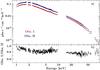 |
Fig. 7 a) Unfolded phase-averaged spectra of Obs. I (red) and Obs. II (blue) and b) ratio of the phase-averaged spectra of Obs. I and Obs. II. For clarity, only XIS3, PIN and GSO data are shown in both panels. The ratios of the individual detectors have been corrected for the respective cross-calibration constants given in Table 2. |
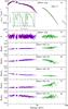 |
Fig. 8 Panels a) and b): phase-averaged spectrum of XIS0 (blue), XIS1 (red), XIS3 (magenta), PIN (green), and GSO (brown) of Obs. I with best-fit model and residuals. Panels c) through g): count rates of the respective phase-resolved spectra (1) to (5), divided by the count rate of the phase-averaged spectrum. |
Figure 7 shows the unfolded spectra of Obs. I and Obs. II in comparison and the photon ratio of both observations. We observe a slight change in spectral slope below ~2.5 keV, while the ratio is mainly flat above this energy with slight differences in the Fe band. Above the cyclotron line energy the spectra are very similar in shape. Comparing the fit parameters of both Suzaku observations, we find a decrease of the photon index and folding energies toward higher flux. Fürst et al. (2014) observed the opposite trend regarding the first and second NuSTAR observation. There is, however, an artificial correlation between these two parameters, which is not taken into account here, so we cannot conclude that the Suzaku and NuSTAR results contradict each other. The excess of soft photons in Obs. I below ~2.5 keV is at least partly explained by the increase of the blackbody temperature from Obs. I to Obs. II, while the relative normalization of the blackbody component is very similar in both observations. This behavior is consistent with NuSTAR. See Fürst et al. (2014) for a more detailed investigation of the parameter evolution over the outburst.
The fitted NH value is comparable to the value of 0.89 × 1022 cm-2 given by the Leiden/Argentine/Bonn (LAB) Survey of Galactic HI (Kalberla et al. 2005).
5. Phase-resolved spectroscopy
We extracted spectra for five individual pulse phase intervals (Phase bin [Pb] 1–5; see Fig. 3 for definition of phase intervals) to study the variation of the continuum with the viewing angle onto the neutron star. The width and location of the phase intervals were chosen to ensure sufficient S/N as well as to distinguish the most characteristic features of the pulse profiles. In order to account for lower statistics due to splitting the observations into phase bins, we reduced the required minimum S/N for rebinning the XIS spectra to 50 (45 for 6–7 keV) for all phase intervals with exception of the phase interval covering the pulse profile minimum (Pb 3), where we required a minimum S/N of 40 (35 for 6–7 keV). The PIN spectra were rebinned to a minimum S/N of 15. We ignored the GSO spectra for the phase-resolved analysis because of their low statistics.
We first calculated the ratio of all phase-resolved spectra with respect to the phase-averaged spectrum, allowing us to investigate the evolution of the phase-resolved spectra in a model-independent way (Fig. 8). The spectrum of Pb 1 is most similar in shape to the phase-averaged spectrum, which is not surprising as this phase interval covers the peak of the main pulse and, therefore, contributes heavily to the phase-averaged spectrum. All other ratios indicate changes in spectral shape. The spectrum of the main minimum (Pb 3) is softer than that of the main pulse and the spectrum of the emerging peak (Pb 4) is harder. The differences of the main pulse spectrum with respect to the spectra of the declining main pulse (Pb 2) and the emerging minimum (Pb 5) are more complex.
We used the same spectral model for the phase-resolved as for the phase-averaged analysis, but without the H-like iron emission for the first observation. Since we expect the detector cross-calibration constants and the iron line energies to be independent of the viewing angle onto the neutron star, these were constrained to be the same for all phase intervals. On our final fits, these parameters were identical to those of the phase-averaged analysis to within their confidence intervals. All other parameters were fitted individually for each phase interval.
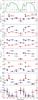 |
Fig. 9 Evolution of the best-fit parameters of Obs. I (red) and Obs. II (blue) over pulse phase. Upper panel: PIN pulse profile of Obs. II over its complete energy range. Dashed lines indicate the selected phase intervals. All fluxes (a) are given in units of 10-9 erg s-1 cm-2. Profiles and parameter evolutions are shown twice for clarity. |
Figure 9 presents the evolution of some of the fit parameters over pulse phase for both observations. We observe variations for all continuum parameters and of the CRSF strength over pulse phase. Variations of the hard power-law flux ℱ15−50 keV, blackbody flux ℱBB, and iron line flux (not shown) mostly follow the pulse profile. Trends are generally the same for Obs. I and Obs. II, while absolute parameter values can be moderately different. We calculated confidence contours for two parameters of interest for several parameter pairs to evaluate the significance of parameter differences in the presence of possible artificial dependencies; see Fig. 10.
The emerging minimum (Pb 5) shows the highest absorption and the main minimum (Pb 3) shows the lowest absorption and comparatively weak and cool blackbody. These two phase bins generally display the most distinct changes compared to their neighbors. The contour plots confirm that the difference in NH between the two extremes is significant. Regarding the blackbody temperature they reveal that, with exception of the main minimum, the phase intervals are consistent with a kTBB of ~0.6 keV and ~0.7 keV for the first and second observation, respectively2. Changes of the absorption column and blackbody temperature could not be constrained by the >3 keV phase-resolved NuSTAR analysis, where NH was fixed to 0.845 × 1022 cm-2 and kTBB to ~0.6 keV (Fürst et al. 2014).
Confirming the picture obtained from the spectral ratios of Fig. 8, the phase variation of Γ shows that the power law is comparatively soft during the main minimum (Pb 3) and the emerging minimum (Pb 5). For Obs. I, the contours show that the softest and hardest Γ values are indeed significantly different from each other. The folding energy is roughly correlated with Γ. The Efold-Γ contours reveal that this variation is at least in part due to the model intrinsic correlation between these two parameters. Our results indicate that Γ and Efold are high during the secondary minimum (Pb 5) and that the CRSF is strongest during the main minimum (Pb 3) and secondary peak (Pb 4), which is qualitatively consistent with the higher resolution NuSTAR analysis (20 phase bins, Fürst et al. 2014). The NuSTAR analysis also found a slight softening during the main minimum.
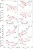 |
Fig. 10 Contour maps showing the 3σ confidence regions for the phase-resolved spectra of both observations. Top: blackbody temperature and flux versus NH. Bottom: folding energy Efold and blackbody flux versus photon index Γ. Tied parameters (iron line energies and detector cross-normalization constants) were held constant for the calculation. The labels (1)–(5) indicate the respective phase interval. |
6. Discussion and conclusions
In this paper we reported on spectral and timing analyses of two observations of the 2013 outburst of KS 1947+300. The phase-averaged spectrum shows emission features at energies ~6.4 keV, ~6.7 keV, and, for the first observation, also at ~6.9 keV, which we interpret as Kα emission from neutral, He-like, and H-like iron. This is the first time lines from different ionization states of iron are detected in this source. The neutral line could also be a blend of other ionization states, which cannot be distinguished with the available data.
Observations of the 2000/2001 outburst already found indications for the presence of neutral (Tsygankov & Lutovinov 2005, with RXTE) or He-like iron (Naik et al. 2006, with BeppoSAX), however, none of these observations showed the different ionization stages at the same time, probably owing to the lower energy resolution of the earlier instruments. NuSTAR, with an energy resolution that is a factor of ~2 worse than the XIS, only detected one line feature at 6.5 keV, hinting at the presence of ionization features (Fürst et al. 2014), similar to the variability of the line energy seen with RXTE (Tsygankov & Lutovinov 2005). The accreting pulsar that is best known for showing emission lines from neutral, He-like and H-like iron is the persistent source Cen X-3, where the individual line strengths vary over the binary orbit, constraining different emission regions (Naik et al. 2011a).
Although the ~12.2 keV center energy of the cyclotron line is not covered by the Suzaku instruments, this feature was included in the spectral model because the line wings affect the spectral shape. The correction due to the cyclotron line is most prominent during the pulse minimum and the emerging second peak, which is consistent with the NuSTAR-detected line variability (Fürst et al. 2014).
Consistent with earlier observations (e.g., Naik et al. 2006), the pulse profiles are highly energy dependent, in particular, we observe the evolution from one broad peak to one broad and one narrow peak toward higher energies. Many neutron star binaries show the opposite behavior with peaks vanishing at high energies, e.g., 4U 0115+634 (Müller et al. 2010), 4U 1909+07 (Fürst et al. 2011), Vela X-1 (Kreykenbohm et al. 2002), GX 304−1 (Devasia et al. 2011), 1A 1118−61 (Suchy et al. 2011; Maitra et al. 2012), GRO J1008−57 (Naik et al. 2011b), or EXO 2030+375 (Naik et al. 2013). We note, however, that IGR J16393−4643 shows an evolution with energy that is similar to that in KS 1947+300 (Islam et al. 2015). Islam et al. (2015) suggest that either additional soft photons from off-pulse regions or a more direct view into the emission region at the peak are the reason for the observed spectral variation.
The characteristic narrow and sharp peak observed in the pulse profiles of KS 1947+300 could be caused by relativistic light bending effects, allowing constraints on the inclination of the observer and the magnetic field. Such parameters are generally very difficult to determine. Any additional information on the geometry of the system, as provided, e.g., by a sharp feature, reduces the number of free parameters and thus simplifies the modeling of the pulse profiles. The energy dependence might be caused by an energy-dependent beam pattern and contributions from the accretion column, the neutron star surface, and a surrounding halo (Kraus et al. 1989, 2003; Falkner 2013). A quantitative modeling of the pulse profiles is, however, beyond the scope of this paper and will be presented in a forthcoming publication.
The high sensitivity of Suzaku XIS in the soft X-rays additionally allows us to investigate spectral variation over pulse phase below 3 keV. We find the spectrum to be softer during the two minimum phases Pb 3 and Pb 5. Despite strong correlations between the continuum parameters (Fig. 10), the soft spectrum during Pb 3 appears to be due to a combination of a lower NH together with a softening of the underlying continuum. If true, this overall phase dependence of NH would imply the presence of at most moderately ionized material that is located close to the neutron star and coupled to its magnetic field. In our model, we use a neutral absorption component, which is a common approach in accreting X-ray pulsars. This is valid because most of the absorption happens by K-shell electrons, so a moderately ionized medium can still be successfully modeled with a neutral absorber. We also applied the analytic warmabs model as part of the XSTAR3 software package and found that an ionized absorber does not improve our fit significantly in terms of χ2 and the resulting ionization fractions are very low in both observations (log ξ ~ −0.05).
While the general dependence of the spectral properties on pulse phase is in line with results from the 2000/2001 outburst (Galloway et al. 2004; Naik et al. 2006), our results differ in that no NH variability was seen in the older data. It is well known that NH in accreting neutron stars strongly depends on the assumed underlying continuum model (see, e.g., the modeling of the NH variability of 4U 1538−522; Hemphill et al. 2014). A possible explanation for this discrepancy could therefore be that the pulse phase variability of the earlier outburst was described by the variation of the optical depth and temperature of a thermal Comptonization model (compTTHua & Titarchuk 1995) to which a soft blackbody was added. This approach indeed resulted in much lower NH values (NH ~ 5 × 1021 cm-2, i.e., the minimum NH detectable with the RXTE-PCA, but well within the range accessible by BeppoSAX; Galloway et al. 2004; Naik et al. 2006). Our attempts to model the 2013 data with a Comptonization continuum resulted in a barely acceptable fit ( for Obs. I and
  for Obs. II), and even though NH turned out to be comparable with the 2000/2001 values, the fits still showed a similar pulse phase dependency of NH to that found with the empirical models employed in Sect. 5.
A next step in describing the data would be to replace empirical models such as our approach or single temperature Comptonization models with a fully self-consistent description of the physical processes in the accretion column (e.g., Becker & Wolff 2007, and references therein). The publicly available XSPEC model compmag (Farinelli et al. 2012) provides a numerical solution of the equation of radiative transfer given in Becker & Wolff (2007) modified by a second order bulk Componization term and allowing for other velocity profiles than considered in Becker & Wolff (2007). We have tried to fit the compmag model to the phase-averaged spectra, which turned out not to describe the data successfully. We note, however, the compmag model uses a blackbody seed spectrum to be convolved with the Green’s function, whereas in the full Becker & Wolff (2007) model, bremsstrahlung and cyclotron emission also contribute to the seed spectrum, which play a dominant role at high luminosities. The compmag model is therefore rather applicable to low luminosity observations and does not fit the bright observations of KS 1947+300 very well. Members of our team are currently in the process of preparing an implementation of the full model of Becker & Wolff (2007). An independent implementation of the Becker & Wolff (2007) model, together with a thermal Comptonization component has been applied successfully to the spectrum of 4U 0115+634 by Ferrigno et al. (2009).
For a full picture of the accretion mechanism, combined spectral and timing analysis is required. The self-consistent modeling of both the spectra and pulse profiles will finally allow us to disentangle artificial parameter correlations and track physical properties over pulse phase. This is, however, a very challenging undertaking owing to the large number of free parameters and because the required computing time is very high in both the spectral and geometrical models. Huge efforts in developing and improving these models have been made for several years now and we are still at a point where every successful application to observational data provides a valuable example. KS 1947+300 seems to be a promising candidate for more dedicated studies and we hope that additional constraints on the source geometry will eventually help to improve our understanding of the spectral and angular redistribution of radiation inside the accretion column.
The individual NH-kTBB and NH-ℱBB contours reveal artificial parameter dependencies in the sense that higher values of NH correspond to lower blackbody temperatures and fluxes, although at first glance one might expect the absorption component to “compensate” for emission in the soft range. The individual Γ-ℱBB contours show that the trade-off happens with a softer power law instead.
Acknowledgments
We thank the anonymous referee for very constructive comments that helped us to improve the quality of the paper. We acknowledge funding by the Bundesministerium für Wirtschaft und Technologie under Deutsches Zentrum für Luft- und Raumfahrt grants 50OR1113 and 50OR1207. V.G. acknowledges support provided by NASA through the Smithsonian Astrophysical Observatory (SAO) contract SV3-73016 to MIT for support of the Chandra X-Ray Center (CXC) and Science Instruments; CXC is operated by SAO for and on behalf of NASA under contract NAS8-03060. We thank John E. Davis for the development of the SLXfig module, which was used to create all figures presented in this paper. This research has made use of ISIS functions (isisscripts) provided by ECAP/Remeis observatory and MIT4.
References
- Becker, P. A., & Wolff, M. T. 2007, ApJ, 654, 435 [NASA ADS] [CrossRef] [Google Scholar]
- Boldt, E. 1987, in Observational Cosmology, eds. A. Hewitt, G. Burbidge, & L. Z. Fang, IAU Symp. 124 (Dordrecht: Reidel), 611 [Google Scholar]
- Borozdin, K., Gilfanov, M., Sunyaev, R., et al. 1990, Sov. Astron. Lett., 16, 345 [NASA ADS] [Google Scholar]
- Chakrabarty, D., Koh, T., Bildsten, L., et al. 1995, ApJ, 446, 826 [NASA ADS] [CrossRef] [Google Scholar]
- Devasia, J., James, M., Paul, B., & Indulekha, K. 2011, MNRAS, 417, 348 [NASA ADS] [CrossRef] [Google Scholar]
- Falkner, S. 2013, Master’s thesis, University of Erlangen-Nuremberg [Google Scholar]
- Farinelli, R., Ceccobello, C., Romano, P., & Titarchuk, L. 2012, A&A, 538, A67 [NASA ADS] [CrossRef] [EDP Sciences] [Google Scholar]
- Ferrigno, C., Becker, P. A., Segreto, A., Mineo, T., & Santangelo, A. 2009, A&A, 498, 825 [NASA ADS] [CrossRef] [EDP Sciences] [Google Scholar]
- Ferrigno, C., Falanga, M., Bozzo, E., et al. 2011, A&A, 532, A76 [NASA ADS] [CrossRef] [EDP Sciences] [Google Scholar]
- Fukazawa, Y., Mizuno, T., Watanabe, S., et al. 2009, PASJ, 61, 17 [NASA ADS] [Google Scholar]
- Fürst, F., Kreykenbohm, I., Suchy, S., et al. 2011, A&A, 525, A73 [NASA ADS] [CrossRef] [EDP Sciences] [Google Scholar]
- Fürst, F., Pottschmidt, K., Wilms, J., et al. 2014, ApJ, 784, L40 [NASA ADS] [CrossRef] [Google Scholar]
- Galloway, D. K., Morgan, E. H., & Levine, A. M. 2004, ApJ, 613, 1164 [NASA ADS] [CrossRef] [Google Scholar]
- Harding, A. K., & Lai, D. 2006, Rep. Prog. Phys., 69, 2631 [NASA ADS] [CrossRef] [Google Scholar]
- Heindl, W. A., Coburn, W., Gruber, D. E., et al. 1999, ApJ, 521, L49 [NASA ADS] [CrossRef] [Google Scholar]
- Hemphill, P. B., Rothschild, R. E., Markowitz, A., et al. 2014, ApJ, 792, 14 [NASA ADS] [CrossRef] [Google Scholar]
- Houck, J. C., & Denicola, L. A. 2000, in Astronomical Data Analysis Software and Systems IX, eds. N. Manset, C. Veillet, & D. Crabtree, ASP Conf. Ser. 216, 591 [Google Scholar]
- Hua, X.-M., & Titarchuk, L. 1995, ApJ, 449, 188 [NASA ADS] [CrossRef] [Google Scholar]
- Islam, N., Maitra, C., Pradhan, P., & Paul, B. 2015, MNRAS, 446, 4148 [NASA ADS] [CrossRef] [Google Scholar]
- Kalberla, P. M. W., Burton, W. B., Hartmann, D., et al. 2005, A&A, 440, 775 [NASA ADS] [CrossRef] [EDP Sciences] [Google Scholar]
- Koyama, K., Tsunemi, H., Dotani, T., et al. 2007, PASJ, 59, 23 [Google Scholar]
- Kraus, U., Herold, H., Maile, T., Nollert, H.-P., & Rebetzky, A. 1989, A&A, 223, 246 [NASA ADS] [Google Scholar]
- Kraus, U., Zahn, C., Weth, C., & Ruder, H. 2003, ApJ, 590, 424 [NASA ADS] [CrossRef] [Google Scholar]
- Kreykenbohm, I., Coburn, W., Wilms, J., et al. 2002, A&A, 395, 129 [NASA ADS] [CrossRef] [EDP Sciences] [Google Scholar]
- Krimm, H. A., Holland, S. T., Corbet, R. H. D., et al. 2013, ApJS, 209, 14 [NASA ADS] [CrossRef] [Google Scholar]
- Leahy, D. A., Darbro, W., Elsner, R. F., et al. 1983, ApJ, 266, 160 [NASA ADS] [CrossRef] [Google Scholar]
- Levine, A., & Corbet, R. 2000, IAU Circ. 7523 [Google Scholar]
- Madsen, K. K., Harrison, F. A., Markwardt, C., et al. 2015, ApJS, 220, 8 [NASA ADS] [CrossRef] [Google Scholar]
- Maitra, C., Paul, B., & Naik, S. 2012, MNRAS, 420, 2307 [NASA ADS] [CrossRef] [Google Scholar]
- Müller, S., Obst, M., Kreykenbohm, I., et al. 2010, PoS(INTEGRAL 2010)116 [Google Scholar]
- Naik, S., Callanan, P. J., Paul, B., & Dotani, T. 2006, ApJ, 647, 1293 [NASA ADS] [CrossRef] [Google Scholar]
- Naik, S., Paul, B., & Ali, Z. 2011a, ApJ, 737, 79 [NASA ADS] [CrossRef] [Google Scholar]
- Naik, S., Paul, B., Kachhara, C., & Vadawale, S. V. 2011b, MNRAS, 413, 241 [NASA ADS] [CrossRef] [Google Scholar]
- Naik, S., Maitra, C., Jaisawal, G. K., & Paul, B. 2013, ApJ, 764, 158 [NASA ADS] [CrossRef] [Google Scholar]
- Negueruela, I., Israel, G. L., Marco, A., Norton, A. J., & Speziali, R. 2003, A&A, 397, 739 [NASA ADS] [CrossRef] [EDP Sciences] [Google Scholar]
- Nowak, M. A., Hanke, M., Trowbridge, S. N., et al. 2011, ApJ, 728, 13 [NASA ADS] [CrossRef] [Google Scholar]
- Ozawa, M., Uchiyama, H., Matsumoto, H., et al. 2009, PASJ, 61, 1 [NASA ADS] [Google Scholar]
- Palmeri, P., Mendoza, C., Kallman, T. R., Bautista, M. A., & Meléndez, M. 2003, A&A, 410, 359 [NASA ADS] [CrossRef] [EDP Sciences] [Google Scholar]
- Pottschmidt, K., Kreykenbohm, I., Wilms, J., et al. 2005, ApJ, 634, L97 [NASA ADS] [CrossRef] [Google Scholar]
- Protassov, R., van Dyk, D. A., Connors, A., Kashyap, V. L., & Siemiginowska, A. 2002, ApJ, 571, 545 [NASA ADS] [CrossRef] [Google Scholar]
- Schönherr, G., Schwarm, F.-W., Falkner, S., et al. 2014, A&A, 564, L8 [NASA ADS] [CrossRef] [EDP Sciences] [Google Scholar]
- Suchy, S., Pottschmidt, K., Wilms, J., et al. 2008, ApJ, 675, 1487 [NASA ADS] [CrossRef] [Google Scholar]
- Suchy, S., Pottschmidt, K., Rothschild, R. E., et al. 2011, ApJ, 733, 15 [NASA ADS] [CrossRef] [Google Scholar]
- Swank, J., & Morgan, E. 2000, IAU Circ. 7531 [Google Scholar]
- Takahashi, T., Abe, K., Endo, M., et al. 2007, PASJ, 59, 35 [NASA ADS] [CrossRef] [EDP Sciences] [Google Scholar]
- Tendulkar, S. P., Fürst, F., Pottschmidt, K., et al. 2014, ApJ, 795, 154 [NASA ADS] [CrossRef] [Google Scholar]
- Tsujimoto, M., Guainazzi, M., Plucinsky, P. P., et al. 2011, A&A, 525, A25 [NASA ADS] [CrossRef] [EDP Sciences] [Google Scholar]
- Tsygankov, S. S., & Lutovinov, A. A. 2005, Astron. Lett., 31, 88 [NASA ADS] [CrossRef] [Google Scholar]
- Uchiyama, Y., Maeda, Y., Ebara, M., et al. 2008, PASJ, 60, 35 [NASA ADS] [Google Scholar]
- Verner, D. A., Ferland, G. J., Korista, K. T., & Yakovlev, D. G. 1996, ApJ, 465, 487 [NASA ADS] [CrossRef] [Google Scholar]
- Wilms, J., Allen, A., & McCray, R. 2000, ApJ, 542, 914 [NASA ADS] [CrossRef] [Google Scholar]
- Yamada, S., Makishima, K., Nakazawa, K., et al. 2011, PASJ, 63, 645 [NASA ADS] [Google Scholar]
All Tables
All Figures
|
Fig. 1 Swift/BAT daily light curve in the 15–50 keV band of the outburst in 2013. The blue vertical lines indicate the times covered by Suzaku observations. |
| In the text | |
|
Fig. 2 Light curve and hardness ratio of XIS3 of both observations with 128 s time bins. The light curve covers the energy range 1–10 keV. The hardness ratio is defined as the ratio of the count rate in the 7–10 keV band to the count rate in the 1–4 keV band. |
| In the text | |
|
Fig. 3 Background-subtracted pulse profiles of Obs. I. The upper panel shows the PIN profiles with the phase intervals chosen for phase-resolved spectral analysis. The lower panel shows the XIS0 (blue), XIS1 (red), XIS3 (magenta) profiles. The pulse profiles are very similar to those of Obs. II. All profiles are shown twice for clarity. |
| In the text | |
|
Fig. 4 Color-coded map of the count rate distribution of the NuSTAR observation as a function of energy and pulse phase. Each row represents a normalized pulse profile at the respective energy and each column, technically, indicates a phase-resolved spectrum. All profiles are shown twice for clarity. |
| In the text | |
|
Fig. 5 a) Phase-averaged spectrum of Obs. II with best-fit model: XIS0 (blue), XIS1 (red), XIS3 (magenta), PIN (green) and GSO (brown). b) Residuals of continuum model without CRSF and Fe lines. c) Residuals of continuum model with narrow Kα and Kβ lines of neutral iron only and CRSF. d) Residuals of continuum model with both neutral and He-like Fe lines but without CRSF. e) Residuals of best-fit model including CRSF and Fe-lines. |
| In the text | |
|
Fig. 6 Close-up plot of the iron line region for Obs. I. Panel a): XIS0 (blue), XIS1 (red), and XIS3 (magenta) data with the best-fitting model (black). Panel b): residuals for the continuum model only, i.e., without any emission lines. Panel c): residuals for the continuum model with the Kα line of neutral iron and panel d): residuals for the continuum model with both, neutral and He-like, Kα lines. Panel e): residuals for the continuum model with lines from neutral, He-like, and H-like iron included. All panels show the best fit for the respective model. |
| In the text | |
|
Fig. 7 a) Unfolded phase-averaged spectra of Obs. I (red) and Obs. II (blue) and b) ratio of the phase-averaged spectra of Obs. I and Obs. II. For clarity, only XIS3, PIN and GSO data are shown in both panels. The ratios of the individual detectors have been corrected for the respective cross-calibration constants given in Table 2. |
| In the text | |
|
Fig. 8 Panels a) and b): phase-averaged spectrum of XIS0 (blue), XIS1 (red), XIS3 (magenta), PIN (green), and GSO (brown) of Obs. I with best-fit model and residuals. Panels c) through g): count rates of the respective phase-resolved spectra (1) to (5), divided by the count rate of the phase-averaged spectrum. |
| In the text | |
|
Fig. 9 Evolution of the best-fit parameters of Obs. I (red) and Obs. II (blue) over pulse phase. Upper panel: PIN pulse profile of Obs. II over its complete energy range. Dashed lines indicate the selected phase intervals. All fluxes (a) are given in units of 10-9 erg s-1 cm-2. Profiles and parameter evolutions are shown twice for clarity. |
| In the text | |
|
Fig. 10 Contour maps showing the 3σ confidence regions for the phase-resolved spectra of both observations. Top: blackbody temperature and flux versus NH. Bottom: folding energy Efold and blackbody flux versus photon index Γ. Tied parameters (iron line energies and detector cross-normalization constants) were held constant for the calculation. The labels (1)–(5) indicate the respective phase interval. |
| In the text | |
Current usage metrics show cumulative count of Article Views (full-text article views including HTML views, PDF and ePub downloads, according to the available data) and Abstracts Views on Vision4Press platform.
Data correspond to usage on the plateform after 2015. The current usage metrics is available 48-96 hours after online publication and is updated daily on week days.
Initial download of the metrics may take a while.