| Issue |
A&A
Volume 588, April 2016
|
|
|---|---|---|
| Article Number | A23 | |
| Number of page(s) | 17 | |
| Section | Extragalactic astronomy | |
| DOI | https://doi.org/10.1051/0004-6361/201526397 | |
| Published online | 11 March 2016 | |
Molecular gas in low-metallicity starburst galaxies:
Scaling relations and the CO-to-H2 conversion factor⋆
1 INAF–Osservatorio Astronomico di Roma, via Frascati 33, 00040 Monte Porzio Catone, Roma, Italy
e-mail: This email address is being protected from spambots. You need JavaScript enabled to view it.
2 Instituto de Astrofísica de Canarias (IAC), vía Láctea S/N, 38200 La Laguna, Tenerife, Spain
3 Departamento de Astrofísica, Universidad de La Laguna, 38206 La Laguna, Tenerife, Spain
4 Observatorio Astronómico Nacional (IGN), Alfonso XII 3, 28014 Madrid, Spain
Received: 24 April 2015
Accepted: 16 December 2015
Abstract
Context. Tracing the molecular gas-phase in low-mass star-forming galaxies becomes extremely challenging due to significant UV photo-dissociation of CO molecules in their low-dust, low-metallicity ISM environments.
Aims. We aim to study the molecular content and the star-formation efficiency of a representative sample of 21 blue compact dwarf galaxies (BCDs), previously characterized on the basis of their spectrophotometric properties.
Methods. We present CO (1–0) and (2–1) observations conducted at the IRAM-30m telescope. These data are further supplemented with additional CO measurements and multiwavelength ancillary data from the literature. We explore correlations between the derived CO luminosities and several galaxy-averaged properties.
Results. We detect CO emission in seven out of ten BCDs observed. For two galaxies these are the first CO detections reported so far. We find the molecular content traced by CO to be correlated with the stellar and Hi masses, star formation rate (SFR) tracers, the projected size of the starburst, and its gas-phase metallicity. BCDs appear to be systematically offset from the Schmidt-Kennicutt (SK) law, showing lower average gas surface densities for a given ΣSFR, and therefore showing extremely low (≲0.1 Gyr) H2 and H2 +Hi depletion timescales. The departure from the SK law is smaller when considering H2 +Hi rather than H2 only, and is larger for BCDs with lower metallicity and higher specific SFR. Thus, the molecular fraction (ΣH2/ ΣHI) and CO depletion timescale (ΣH2/ ΣSFR) of BCDs is found to be strongly correlated with metallicity. Using this, and assuming that the empirical correlation found between the specific SFR and galaxy-averaged H2 depletion timescale of more metal-rich galaxies extends to lower masses, we derive a metallicity-dependent CO-to-H2 conversion factor αCO,Z ∝ (Z/Z⊙)− y, with y = 1.5(±0.3)in qualitative agreement with previous determinations, dust-based measurements, and recent model predictions. Consequently, our results suggest that in vigorously star-forming dwarfs the fraction of H2 traced by CO decreases by a factor of about 40 from Z ~ Z⊙ to Z ~ 0.1 Z⊙, leading to a strong underestimation of the H2 mass in metal-poor systems when a Galactic αCO,MW is considered. Adopting our metallicity-dependent conversion factor αCO,Z we find that departures from the SK law are partially resolved.
Conclusions. Our results suggest that starbursting dwarfs have shorter depletion gas timescales and lower molecular fractions compared to normal late-type disc galaxies, even accounting for the molecular gas not traced by CO emission in metal-poor environments, raising additional constraints to model predictions.
Key words: galaxies: ISM / radio lines: ISM / galaxies: starburst / galaxies: evolution / galaxies: general
Based on observations carried out with the IRAM 30m Telescope. IRAM is supported by INSU/CNRS (France), MPG (Germany) and IGN (Spain).
© ESO, 2016
1. Introduction
Blue compact galaxies (BCDs) are low luminosity gas-rich systems with an optical extent of a few kpc (Thuan & Martin 1981). They undergo intense bursts of star formation, as evidenced by their blue colours and strong nebular emission, with ongoing star-formation rates (SFR) typically ~0.1−10 M⊙ yr-1 (e.g., Gil de Paz et al. 2003). BCDs span a wide range of sub-solar metallicities 0.02 ≲ Z/Z⊙ ≲ 0.5), including the most metal-poor star-forming galaxies known in the local Universe (e.g., Terlevich et al. 1991; Kunth & Östlin 2000; Kniazev et al. 2004; Izotov et al. 2006; Papaderos et al. 2006, 2008; Morales-Luis et al. 2011; Filho et al. 2013). These extreme properties originally lead to conjecture that they are pristine galaxies that, at present, are experiencing the formation of their first stellar population (Sargent & Searle 1970). Subsequent work has shown, however, that most (>95%) BCDs are old systems (>5 Gyr) that have undergone previous starburst episodes (Gerola et al. 1980; Davies & Phillipps 1988; Sánchez Almeida et al. 2008). This conclusion relies mostly upon the detection of a more extended, evolved low-surface brightness host galaxy (Papaderos et al. 1996a,b; Cairós et al. 2001a, 2003; Noeske et al. 2003, 2005; Caon et al. 2005; Gil de Paz & Madore 2005; Vaduvescu et al. 2006; Hunter & Elmegreen 2006; Amorín et al. 2007, 2009; Micheva et al. 2013). Nonetheless, even though they are not pristine galaxies, nearby BCDs constitute ideal laboratories for studying vigorous star formation and galaxy evolution in great detail, under physical conditions that are comparable to those present in low-mass galaxies at higher redshift (e.g., Amorín et al. 2015, 2014a,b; Maseda et al. 2014; de Barros et al. 2016).
So far, our understanding of the main processes triggering and regulating star formation activity in BCDs remains very limited. This is largely due to our poor knowledge of the physical mechanisms behind starburst activity, as well as of the feedback induced by the massive star formation in the interstellar medium (ISM). The strong UV radiation and the mechanical energy from stellar winds and SNe are likely agents of feedback in starbursts like those present in BCDs, leading to the ejection of metal-enriched gas into the galactic halo, which limits the star formation and shapes the large-scale structure and kinematics of the surrounding ISM (e.g., Mac Low & Ferrara 1999; Silich & Tenorio-Tagle 2001; Tenorio-Tagle et al. 2006; Recchi & Hensler 2013).
Likewise, the triggering of the starburst in BCDs remains a puzzle: these low-mass, gas-rich galaxies generally lack density waves and only a small fraction of them are seen in strong tidal interactions or merging with more massive companions (e.g., Campos-Aguilar et al. 1993; Telles & Terlevich 1995; Pustilnik et al. 2001; Koulouridis et al. 2013). The origin of their ongoing star-formation activity has been predominantly associated with fainter interactions with low-mass companions (e.g., Noeske et al. 2001; Brosch et al. 2004; Bekki 2008), cold-gas accretion (e.g., Sánchez Almeida et al. 2014, 2015), and other, barely understood internal processes (e.g., Papaderos et al. 1996b; van Zee et al. 2001; Hunter & Elmegreen 2004).
Results from detailed surface photometry have shown that starbursting dwarfs are more compact, i.e., they have a higher stellar concentration than more quiescent dwarf irregulars (dIs), (e.g., Papaderos et al. 1996b; Gil de Paz & Madore 2005; Amorín et al. 2009). Moreover, spatially resolved Hi studies (van Zee et al. 1998, 2001; Ekta & Chengalur 2010; López-Sánchez et al. 2012; Lelli et al. 2014a,b) have shown both that the central gas surface density in BCDs can be a factor ≳2 higher and that their Hi gas kinematics is more disturbed than in dIs. Some of these studies suggest that inflows of gas onto a BCD might lead to a critical gas density and, in turn, to the ignition of star formation on a small (~1 kpc) spatial scale. In addition, it has been suggested that gravity-driven motions and torques induced by the formation and further interaction of large star-forming clumps may also lead to central gas accretion and angular momentum loss, feeding the current starburst (Elmegreen et al. 2012). Additional observational support to this picture has been recently provided by studies of chemical abundances and ionized gas kinematics in metal-poor starbursts (e.g., Amorín et al. 2010b, 2012; Zhao et al. 2013; Sánchez Almeida et al. 2013, 2014)
A complete understanding of the above scenarios must take into account the relation between the total gas content and the ongoing SFR. In a classic paper Schmidt (1959) suggested the existence of a power-law relation between gas and SFR volume densities in the Milky Way. Later, this relation was calibrated in terms of surface densities by Kennicutt (1998) for a large number of galaxies, including late-type disks and massive starburst galaxies. The tight correlation found between the disk-averaged SFR and the gas (atomic, molecular or the sum of both) surface density, is a power law usually referred to as the Schmidt-Kennicutt law (hereafter SK law) and is of the type ΣSFR ∝  , with an exponent N typically ranging 1.3–1.5 (e.g., Bigiel et al. 2008; Kennicutt & Evans 2012). Defining the star-formation efficiency (SFE) as the formation rate of massive stars per unit of gas mass that is able to form stars, or SFE ≡ ΣSFR/ Σgas, the above power law implies that galaxies with higher gas surface density will be more efficient at converting gas into stars.
Recent studies have identified the cold molecular gas density as the primary responsible for the observed star-formation rates in star-forming dwarf galaxies (e.g., Bigiel et al. 2008; Schruba et al. 2011). This is in agreement with the fact that massive star clusters occur in giant molecular clouds. The accumulation of large amounts of cold molecular gas would therefore be a prerequisite for the ignition of a starburst, leading to the assumption that galaxies with vigorous star formation must contain large amounts of H2. The knowledge of the H2 mass, spatial distribution and physical conditions is, therefore, essential for understanding the star-formation process itself, its ISM chemistry and the galaxy evolution as a whole. In spite of their relevance and the extensive observational effort conducted over the last decade (see e.g., Leroy et al. 2005, 2011; Bigiel et al. 2008; Bolatto et al. 2011; Schruba et al. 2012; Boselli et al. 2014; Cormier et al. 2014), these remain key open questions for star-forming dwarf galaxies.
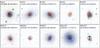 |
Fig. 1 Inverse ugriz color-composite SDSS-DR10 thumbnails of the observed galaxies. Each postage-stamp is 2′ on a side and a standard NE orientation, while the central circle indicates the center and size of the 22′′ CO (J = 1 → 0) beam. |
CO observations.
Owing to the lack of a permanent dipole, H2 emission only arises from hot or warm gas. For this reason, indirect methods are used to estimate the mass of the cold H2 phase of the ISM. The most widely applied tracer is the CO rotational line emission. However, the cold phase of H2, as traced by the 12CO molecule at millimetre wavelengths, seems to be mostly elusive in galaxies with metallicity below ~20% solar (e.g., Elmegreen et al. 2013; Rubio et al. 2015). In particular, BCDs are not only metal-poor but also strongly star-forming, a combination of properties that seems to disfavour high CO detection rates (≲25%, Israel 2005; Leroy et al. 2005). This problem becomes particularly severe in the lowest-metallicity BCDs (Z ≲ 0.1 Z⊙) for which only upper limits in CO luminosity exists and for which the CO-to-H2 conversion factor XCO seems to be extremely uncertain, e.g., in the most metal-poor BCDs I Zw 18 and SBS 0335-052 (Z ~ 0.02 Z⊙), where even very deep searches for CO have proved fruitless (Leroy et al. 2007; Hunt et al. 2014).
Low metallicity environments imply lower C and O abundances and low dust-to-gas ratios (Draine et al. 2007). This affects the relative CO to H2 abundances since dust is the site of H2 formation and also provides much of the far-UV shielding that is necessary to prevent CO – that is not strongly self-shielding – from photodissociating (Bolatto et al. 2013). Most recent model predictions point to a CO deficiency in low-metallicity star-forming galaxies as being due to a decrease in dust-shielding, which leads to strong photo-dissociation of CO by the intense UV radiation fields that are generated in the star-forming regions (e.g., Wolfire et al. 2010; Gnedin & Kravtsov 2010; Glover & Mac Low 2011). Most of these models predict that, while the H2 clouds survive – via self-shielding or dust shielding – in extreme, metal-poor ISM conditions, CO molecules are increasingly destroyed and, therefore, the conversion factor XCO depends strongly on the dust content and metallicity (e.g., Pelupessy & Papadopoulos 2009; Wolfire et al. 2010; Glover & Mac Low 2011; Glover & Clark 2012; Krumholz et al. 2011; Dib 2011; Narayanan et al. 2012).
In this paper we discuss the CO gas content and its relation with the main galaxy-averaged properties of a large sample of BCDs that have been previously studied in a series of papers (Amorín et al. 2009, and references therein). To this aim, we present a small survey of the lowest rotational transitions of 12CO for a sample of ten BCDs. These new data and additional CO measurements obtained from the literature for another eleven BCDs, are combined with a large multiwavelength ancillary data including metallicities, stellar and Hi masses and several SFR tracers. These are used to explore scaling relations between the CO luminosity and star formation in BCDs and, in particular, to study the apparent dependence of the molecular and total (Hi+H2) gas depletion timescales with metallicity. In this analysis, we are able to derive a tight power-law relation for XCO and metallicity, valid for vigorously star-forming dwarfs over nearly one order of magnitude in metallicity.
We organize this paper as follows. In Sects. 2 and 3, we describe the sample of galaxies, the CO observations, and the ancillary datasets. In Sect. 4, we present our results, including the derivation of the CO luminosities, masses and surface densities, and we study different correlations with other galaxy-averaged properties, such as metallicity, sizes, and stellar and gas masses. In Sect. 5, we study the position of the BCDs in the star formation laws, while in Sect. 6, we discuss these results in terms of the star-formation efficiency, specific star-formation rate and metallicity. Later, in Sect. 7, we use these results to derive a metallicity-dependent CO-to-H2 conversion factor and derive total molecular masses. We then revisit different scaling relations, which are compared with previous observational studies and discussed in terms of recent models. Finally, in Sect. 8, we summarize our conclusions. Throughout this paper we adopt H0 = 75 km s-1 Mpc-1, Ω0 = 0.3, Ωλ = 0.7, and solar metallicity 12 +log (O/H)= 8.7 (Allende Prieto et al. 2001).
Multiwavelength properties of the observed galaxies.
2. Sample of galaxies and CO observations
The sample of galaxies consists of 21 out of 28 BCD, which are presented and studied by Cairós et al. (2001a,b), and which were characterized later on the basis of their spectrophotometric properties in subsequent works (Cairós et al. 2003, 2007; Caon et al. 2005; Amorín et al. 2007, 2008, 2009; Amorín 2010a). As discussed in these previous studies, this sample was originally selected as being representative of the BCD class. Thus, it covers the entire range of morphological types, luminosities, colors, gas content, star-formation activity and metallicity properties seen in most BCD samples of the literature.
For the present study, we conducted CO observations for a subset of 10 BCDs (hereafter referred to as subsample I). The Sloan Digital Sky Survey (SDSS) false-color thumbnails for these galaxies are shown in Fig. 1. In Table 1, we summarize the basic observational information for the observed galaxies. For the remaining 11 BCDs in the sample (hereafter referred to as subsample II) we have compiled CO measurements from several sources in the literature, as described in Sect. 3.
The observed BCDs have been selected to favor their CO detectability in one or few pointings. They are small in size (optical diameter <2′), with declinations δ> 15° and show blue colours and strong Hα emission in their centres, indicative of the presence of intense star formation activity.
The observations of the 12CO J = 1 → 0 [ν 115 GHz] and J = 2 → 1 [ν 230 GHz] rotational transitions were obtained during April 25–28, 2006 at the IRAM 30 m telescope (Pico Veleta, Spain). The IRAM telescope provides beam sizes (HPBW1) of about 22′′ and 11′′ at 115 GHz and 230 GHz, respectively, which allowed us to measure the CO emission on the sample galaxies over physical sizes between ~1 and 8 kpc. In the most compact objects, where the star-forming regions are located within the host galaxy effective radius (re ~ 1–2 kpc, Amorín et al. 2009), a single central pointing was enough to cover the whole CO emission (see Fig. 1). On the other hand, in more extended BCDs the observed CO emission corresponds only to the most luminous regions of the starbursts, so it may be considered as a lower limit to the total CO emission. For all the observed galaxies our CO observations cover at least ~50% of the projected size of starburst (rSB, see Sect. 3), while for three objects this fraction, 100 × θb/ 2rSB, is ≳100%.
Multiwavelength properties of galaxies from the literature.
A wobbler switching mode was used at a frequency of 0.5 Hz with a beam throw up to 240′′ in azimuth. Two independent SIS receivers at each frequency (A100, B100 at 3 mm and A230, B230 at 1.3mm) were used to observe both polarizations of the CO J = 1→0 and J = 2→1 transitions simultaneously. The receivers were tuned in single side band, using only the lower band (LSB), which improves the calibration procedure and avoids contamination by other spectral lines in the image band, especially in observations of the calibration sources. The SIS receivers were connected to two filter-banks with resolutions of 1 MHz and 4 MHz at 115 GHz and 230 GHz, respectively, which yields velocity resolutions, δυ, of 2.6 km s-1 and 5.2 km s-1, respectively. These backends have 512 channels each, covering a total instantaneous velocity range of 1300 and 2600 km s-1. Pointing and focus were checked before each integration on continuum sources and planets. The pointing accuracy was better than 2.5′′ on average. Calibrations were done using the chopper wheel method, by observing strong radio sources (Orion A, CW Leo, and W51d). System temperatures at both frequencies varied between ~290–470 K, the higher values being due to bad weather conditions. Thus, we obtained a range for the antenna temperature sensitivity of δTrms ~ 5–15 mK.
The CO spectra was reduced using CLASS2 (Buisson et al. 1997). To increase the signal-to-noise ratio (S/N), averaged spectra for each pointing were obtained by weighting multiple scans by a factor of  , where t is the integration time and Tsys is the system temperature. In all cases, baselines of zeroth order were subtracted. The spectra was then scaled to a main-beam brightness temperature,
  , where Feff and Beff were the forward and beam efficiencies appropriate to the epoch of observations. These values were 0.95 and 0.75 at 115 GHz, and 0.91 and 0.52 at 230 GHz. Finally, all spectra were smoothed to a resolution δυ of 5 km s-1 or 10 km s-1, depending on the S/N.
3. Ancillary datasets
One goal of this paper is to investigate scaling relations between the CO emission and global properties of BCDs (e.g., luminosities, SFRs, metallicities). To this end, we collected a large multiwavelength dataset from public archives and from the literature, as summarized in Tables 2 and 3.
We supplemented our CO observations for subsample I with additional measurements for subsample II from different studies in the literature. With the aim of getting the more homogeneous dataset as possible, we compiled the most recent CO (1→0) fluxes, by giving a preference to those derived from observations at the IRAM 30 m telescope, if available.
We retrieved from theGALEX (Martin et al. 2005) archive3 a fully reduced set of far ultraviolet (FUV: λ1530 Å) galaxy images from the All-Sky Imaging Survey (AIS). The angular resolution of the images is about 6′′. Details on the data characteristics can be obtained from Morrissey et al. (2005). After background subtraction, we performed aperture photometry using circular apertures of 22′′, i.e., the same as the CO (1→0) beamsize. FUV luminosities have been corrected for galactic extinction, using the Schlegel, Finkbeiner, & Davis (1998) dust map and the Cardelli et al. (1989) extinction curve, and for dust attenuation using the prescriptions of Buat et al. (2005), i.e., using the FIR to UV flux ratio.
CO measurements.
We use B-band absolute magnitudes from Cairós et al. (2001a). Luminosities and sizes derived for both the BCD host galaxies and their starburst region were taken from the multi-band 2D surface photometry presented by Amorín et al. (2009). From their study we also collected stellar masses, which were derived using the luminosities and colours of the host galaxies and following Bell & de Jong (2001). Typical uncertainties for stellar masses are below a factor of ~2.
In addition, wecollected Hα integrated luminosities LHα from Cairós et al. (2001b), Gil de Paz et al. (2003) and López-Sánchez & Esteban (2010), which have been used to derive Hα-based SFRs. In the case of UM 462 we transformed Hβ integral luminosities from Lagos et al. (2007) to Hα luminosities using the theoretical Balmer ratio, assuming case B recombination with Te = 104 K and ne = 100 cm-3. For the SFRs, we used the calibration given by Kennicutt et al. (2009): ![Mathematical equation: \begin{equation} \label{eq1} {\it SFR}{\rm (H\alpha)} = 7.9 \times 10^{-42} (L_{\rm H\alpha} + 0.0024 L_{\rm TIR}) [\rm{erg \ s}^{-1}] \end{equation}](/articles/aa/full_html/2016/04/aa26397-15/aa26397-15-eq100.png) (1)that accounts for internal dust attenuation using the total infra-red (IR) luminosity, LTIR (Dale & Helou 2002).
(1)that accounts for internal dust attenuation using the total infra-red (IR) luminosity, LTIR (Dale & Helou 2002).
The collected IR data consist in K-band magnitudes4 from the 2MASS extended source catalogue (XSC; Jarrett et al. 2000), and 60 μm and 100 μm fluxes (F60 y F100) from theIRAS Faint Source Catalog (Moshir et al. 1990). The latter were obtained with a beamsize of 1.44′ and 2.94′ respectively, with a pointing error of about 30′′ that was used as the search radius around the central target coordinates. Detections have medium or good quality for most of the galaxies, with uncertainties below ~10%, and only for few galaxies, namely Mrk 324, Mrk 36, or III Zw 107 are the uncertainties between 20% and 30%. We calculated FIR and TIR fluxes and luminosities by following the prescriptions of Helou et al. (1988) and Dale & Helou (2002).
Furthermore, we use the Hi emission line fluxes, line widths, and systemic velocities from Thuan & Martin (1981) and Gordon & Gottesman (1981) (only for Haro 1, Mrk 297 and III Zw 107). The velocity resolution of the data is 13 and 10 km s-1, respectively. We also used 1.4 GHz continuum luminosities derived from the NRAO VLA Sky Survey (NVSS; Condon et al. 1998) total fluxes. The spatial resolution (FWHM) of the NVSS images is 45′′ and the sensitivity limit (rms noise level) is ~0.45 mJy beam-1.
Finally, we collected gas-phase metallicities for the entire BCD sample from the literature. They were derived following the direct (Te) method or strong-line methods that were calibrated through Hii galaxies or Giant Hii regions with good determination of the electron temperature, e.g., using the N2 (≡log([Nii]/Hα)) index and the relations by Pérez-Montero & Contini (2009). Although this was not possible for the entire sample, for some extended BCDs (e.g., Mrk 35, Mrk 297, Mrk 314, III Zw 102, or Mrk 401) instead of the average (integrated) metallicity, we used the metallicity measured in the star-forming regions covered by the CO observations. Taking into account the typical uncertainties associated with different metallicity calibrations and methods, we considered an average uncertainty value of ~0.2 dex.
4. CO emission in blue compact dwarfs
4.1. Detections and line measurements
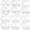 |
Fig. 2 CO detections: CO J = 1 → 0 and J = 2 → 1 spectra are shown for the target galaxies. Horizontal lines indicate the adopted baseline, while vertical lines mark the systemic (heliocentric) velocities as measured from the optical (dotted line) and in 21 cm (dashed lines). The velocity resolution δυ, CO transition, and the name of the galaxy are also labeled in each plot. |
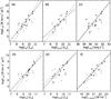 |
Fig. 4 CO luminosity as a function of luminosity in different wavelength bands: Ba), FUVb), Hαc), Kd), FIRe), and 1.4 GHz f). Black and gray points and lines show subsample I and subsample II BCDs, respectively. Arrows indicate CO upper limits. Dashed and solid lines indicate linear fits to detected only and all (detected and non-detected) galaxies, respectively. |
In Table 4 we summarize the results from the CO observations, including values for the CO line velocities, line widths, and integrated fluxes. We detect (≥3σ) CO emission in seven out of ten BCDs: Mrk 33, Mrk 35, Mrk 297, Mrk 401, Haro 1, III Zw 102, and III Zw 107. Two of them, Mrk 401 and III Zw 107, did not present previous CO detections in the literature5. For III Zw 107, we only have 3σ detection at 230 GHz and a marginal detection (<3σ) at 115 GHz after smoothing the spectra to 20 km s-1. For the three remaining galaxies, Mrk 36, and Mrk 324 are not detected, while Mrk 314 shows a tentative ~2σ detection only at 230 GHz, with fluxes in good agreement with previous IRAM observations (Garland et al. 2005). The spectra of the galaxies detected in CO are presented in Fig. 2, while spectra of marginally, or non-detected galaxies, are shown in Fig. 3.
For each detection, a Gaussian function was fitted to the CO emission line to determine the central velocity VCO, the velocity width at half maximum ΔVCO, and the integrated flux ICO = ∫Tmbδυ. For the BCDs that show more than one velocity component, e.g., Mrk 33 or Mrk 35, we fitted up to two Gaussians. For galaxies that show clear asymmetries in the CO line profile, e.g., Mrk 297 or I Zw 102, we have also estimated ICO by the numerical integration of the smoothed spectra within the limits set by the line. In all cases, line flux uncertainties were estimated following Elfhag et al. (1996) and Albrecht et al. (2004). Upper limits for non-detections have been estimated as ICO ≲ 3σ  , where σ is the rms noise level obtained in the baseline range, ΔVCO is the expected total velocity width of the CO line, and δυ is the channel velocity width. For non-detections, we have assumed ΔVCO as the total velocity width of the Hi profile. To check the validity of this approximation, we confirmed that, for clearly detected galaxies, the ratio between CO and Hi line widths is always below one, regardless of the number of Gaussian components.
4.2. CO luminosity
We derive the CO luminosity of the BCD sample as LCO = 23.5Ωobs ICO(1 + z)-3 [K km s-1 pc2] (Solomon et al. 1997), where Ico refers to the CO (1 → 0) integrated fluxes, Ωobs is the observed solid angle at the given frequency and DL is the luminosity distance of the galaxy. The LCO values for the observed galaxies have been listed in Table 4.
From Figs. 4 to 8, we investigate scaling relations between LCO and other key properties that are directly connected to star-formation activity, as well as stellar and gas content in galaxies. In particular, we use luminosities at different wavelengths such as LFUV, LB, LK, LFIR, L1.4 GHz and LHα, stellar (Mstar), and total Hi gas (MHI) masses, effective radius of the host galaxies (re) and projected sizes of the starburst region (rSB), as well as the gas-phase metallicity. Linear least-square fits to data in Figs. 4–8 were performed using the routine fitexy (Press et al. 1992). The results are presented in Table 5.
In Fig. 4 we show the tight correlation found between the CO luminosity and the luminosities in several wavelength bands, most of them classical tracers of the SFR in galaxies. Overall, we find that less luminous BCDs are also fainter in CO. The fitted relations have slopes between ~0.9–1.5. The derived Spearman rank indices ρ (see Table 5) indicate tight correlations between the luminosities considered. The statistical errors provided by the least-square fitting are typically a few %.
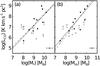 |
Fig. 5 CO luminosity as a function of stellar mass a) and Hi gas mass b). Symbols and colors are as in Fig. 4. |
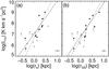 |
Fig. 6 Relation between CO luminosity and effective radius of the host galaxy a), and the size of the starburst emission in the optical b). Symbols and colors are as in Fig. 4. |
In Fig. 5, we also find tentative correlations between the CO luminosity and the total Hi gas mass and stellar mass of the BCD hosts. The latter is in relatively good agreement with the LCO–LK relation, as is expected since the LK is a proxy of stellar mass. Between these two, the relation between LCO and Mstar show a larger scatter, possibly due to larger uncertainties in the derivation of Mstar, i.e., in the colors of the host galaxy and given several assumptions made by models in the derivation of the mass-to-light ratios (e.g., initial mass function or the star-formation history, Amorín et al. 2009).
In Fig. 6 we find that the CO luminosity also scales with size. The correlations between both the effective radius of the host galaxy (re) and the optical size of their starburst (rSB) indicate that larger BCDs, which have extended and luminous starbursts (Amorín et al. 2009), are best detected in CO rather than smaller BCDs with more compact star-forming regions.
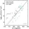 |
Fig. 7 CO luminosity as a function of metallicity. Black dots showsubsample I while open circles showsubsample II, as well as additional very low-metallicity BCDs compiled from the literature (Fumagalli et al. 2010). Green crosses show the compilation of nearby star forming disc galaxies in Krumholz et al. (2009). Lines indicate linear best-fits to all galaxies (solid) and BCDs only (dashed). Error bars indicate typical uncertainties for our sample. |
Finally, in Fig. 7, we show the CO luminosity-metallicity relation. In addition to our galaxy sample, we also include in Fig. 7 CO luminosities for several nearby late-type irregular and spiral galaxies from the literature, including upper limits for the most extremely metal-poor BCDs known, I Zw 18 (Vílchez & Iglesias-Páramo 1998; Leroy et al. 2007) and SBS 0335-052 (Dale et al. 2001; Papaderos et al. 2006). Despite the large scatter, we find a strong positive correlation, which shows the CO luminosity rapidly increasing with metallicity. The same slope is found if we use Ico instead of Lco, in agreement with previous studies (e.g., Taylor et al. 1998; Schruba et al. 2012).
Correlations.
4.3. Molecular mass and surface densities
The molecular hydrogen mass and surface densitytraced by CO can be estimated from CO luminosities. Unfortunately, this implies the assumption of a CO−to−H2 conversion factor, XCO, which strongly depends on the physical conditions of the gas (Bolatto et al. 2013, for an extended review). A frequently used XCO value is obtained from Milky Way virialised molecular clouds. For this reason their use in other galaxies must be taken with caution. This is especially true in metal-poor galaxies, since, as we will discuss later, several observational studies have found XCO as a strong function of metallicity (e.g., Rubio et al. 1993; Wilson 1995; Arimoto et al. 1996; Israel 1997; Leroy et al. 2011; Genzel et al. 2012; Schruba et al. 2012; Bolatto et al. 2013). Keeping this in mind, we have adopted as a first order approach a constant CO-to-H2 conversion factor XCO,MW = 2 × 1020 cm-2 (K km s-1) or αCO,MW = 3.2 M⊙ (K km s-1 pc2)-1 (Strong & Mattox 1996; Dame et al. 2001), which is roughly the mean of values estimated in the Milky Way and nearby galaxies. Including a factor of 1.36 because of the contribution of helium, the total molecular mass traced by CO (in solar units) and the CO surface density (in units of M⊙ pc-2) were then derived as MH2 = 1.36 LCO αCO,MW and ΣH2 = 1.36 cos iαCO,MWICO, where i is the inclination of the galaxies (see Tables 2 and 3).
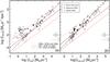 |
Fig. 8 Star-formation rate surface density as a function of H2 (left) and Hi+H2 (right) gas surface densities. Black dots showsubsample I and gray dots showsubsample II. The black dashed lines show the fits to the H2 and H2 +Hi SK law by Leroy et al. (2005) and Shi et al. (2011), respectively. Red lines indicate constant star-formation efficiencies (depletion timescales). Large arrows indicate the shift in H2 surface density by assuming a CO-to-H2 conversion factor 10 times larger than that of the Milky Way for the molecular mass. Error bars indicate typical uncertainties for our sample. |
Using the above prescriptions, our sample of BCDs show a wide range of CO masses, MH2 ~ 2 × 10⁶–4 × 10⁹M⊙, and CO surface densities, ΣH2 ~ 1–170 M⊙ pc-2. Most of these values are typical for late-type irregular and spiral galaxies (cf. e.g., Kennicutt 1998; Leroy et al. 2005), except for the three luminous BCDs of the sample, which are clearly more massive and dense in CO.
5. Star-formation laws
In this section we study the relation between star-formation rates and gas (molecular and neutral) content averaged over the entire starburst region. In addition to the natural interest of further comparing the results provided by studies on sub-kpc scales, studies of BCDs over larger spatial scales can provide an interesting benchmark for future comparison studies with analogues at higher redshifts, for which we can only measure properties at kpc-size scales, even using interferometry.
We explored the position of the BCD sample in the ΣSFR-Σgas plane and compared it with the SK law followed by normal galaxies and luminous starbursts. For that purpose we derived surface densities in Hi (ΣHI), SFR (ΣSFR) and total Hi+H2 gas (Σgas = ΣHI + H2). We followed Kennicutt (1998) and adopted a circular aperture for each galaxy that encloses the region where the star-forming regions are distributed. Thus, for the size of each aperture, we used alternatively r25, rSB, or the CO-beam size after correction for inclination. For the star-formation rate, we considered theongoing SFR, as given by the dust-corrected Hα luminosity. The uncertainties for the SFR and gas surface densities are mainly dominated by possible galaxy-to-galaxy variations in the apertures considered. For the following analysis, we acknowledge a conservative, average uncertainty of ~0.3 dex for surface densities, which do not account by uncertainties in the CO-to-H2 conversion factor and by assumptions involved in the derivation of SFR (e.g., the tracer and IMF in use or the adopted SF history).
In Fig. 8, we present the BCD SFR surface density as a function of their H2 and H2 +Hi surface densities. In this figure, we also included the data (spiral discs and starburst galaxies) used by Kennicutt (1998) for the calibration of the SK law. Instead of including the fit by Kennicutt (1998), we included in Fig. 8a a slightly different fit (ΣSFR = 10-3.4  ) found by Leroy et al. (2005) for a large sample of dwarf irregular galaxies and normal spirals. Similarly, in Fig. 8b, we included the fit presented by Shi et al. (2011) (ΣSFR = 10-3.9
  ) for a larger sample of late-type, early-type, and starburst galaxies at low and high redshift, which includes the sample of galaxies studied by Kennicutt (1998). The relation of Shi et al. (2011) is also in excellent agreement with the more recent update of the SK relation by Kennicutt & Evans (2012).
Overall, Fig. 8 shows the BCD sample located in a region corresponding to depletion timescales for both H2 and H2 +Hi of less than 1 Gyr, which shows surface densities that are smaller than starbusts but larger than spiral and irregulars discs. Remarkably, for most BCDs in our sample, the depletion timescales appear to be up to ~2 dex lower than expected from the SK-laws. In particular, Fig. 8a shows that most BCDs have lower ΣH2 than that predicted by the Leroy et al. (2005) relation for a given ΣSFR. Consequently, their H2 depletion timescales are extremely short (<0.1 Gyr). Considering the total gas (H2 +Hi) surface density, most BCDs still show a systematic departure of up to ~1 dex from the SK relation to low τH2 + HI that is slightly larger than observational uncertainties, as shown in Fig. 8b.
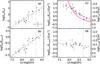 |
Fig. 9 The molecular to atomic ratio a), the molecular fraction b), and the H2 and H2 +Hi depletion timescale (c) and d), respectively) as a function of metallicity. Symbols are as in Fig. 8. Black and gray dashed lines show linear best fits to all data points and only secure detections, respectively. Solid, dotted, and dashed magenta lines in panel c show model predictions by Krumholz et al. (2011) for different values of ΣH2 + HI (80, 20 and 5 M⊙ pc-2, respectively). |
Large offsets from the SK law for metal-poor star-forming galaxies have been reported in previous studies. Rather than galaxies with enhanced SF efficiency or following a distinct SF law, these offsets have been attributed to changes in the CO-to-H2 conversion factor at low metallicities (e.g., Kennicutt & Evans 2012). If instead of using a Galactic conversion factor αCO,MW, we adopt a metallicity-dependent αCO value (e.g., Arimoto et al. 1996), those BCDs with strongly sub-solar metallicities would be displaced to higher gas surface densities and larger depletion timescales (large arrows in Fig. 8). Additional support to this interpretation comes from the most luminous galaxies of the sample, Mrk 297, III Zw 102, and Haro 1, which are the only BCDs that seem to follow the SK relations. These galaxies show significantly higher gas and SFR densities, placing them at the lower end of the trend followed by the IR-selected starbursts of Kennicutt (1998). Up to some point this is not surprising, since these objects are luminous in IR wavelengths, showing clear dust patches/lanes and complex/distorted morphologies in their inner regions (Cairós et al. 2001a,b, see also our Fig. 1) compatible with past or recent mergers. Perhaps most importantly, these galaxies are the most metal-rich starbursts in the sample.
In the following sections we discuss in detail how metallicity affects the molecular gas depletion timescales inextreme ISM conditions (i.e., high ionization and highspecific SFR) of BCDs. This will lead to us finding a method to derive a metallicity-dependent form of αCO that, in turn, allows us to derive corrected H2 masses and revise our scaling relations accordingly.
6. Gas depletion timescales and metallicity
In Fig. 9, we investigate as a function of metallicity the following quantities: (a) the molecular to atomic surface density ratio (i.e., RH2 = ΣH2/ ΣHI); (b) the molecular to total (H2 +Hi) gas surface density ratio (i.e., the molecular fraction fH2 = ΣH2/ ΣH2 + HI) and; (c) and (d) the molecular and total gas (H2 +Hi) SFE and their inverse quantity, the gas depletion timescale τH2 and τH2 + HI, respectively. The coefficients of the best-fit relations, shown in Fig. 9, are presented in Table 5.
In Figs. 9a, b we show that lower RH2 and fH2 are found for BCDs of increasingly lower metallicities. On the other hand, in Fig. 9c we find a strong anticorrelation, showing a fast decrease of the SFE from low- to high-metallicity BCDs. The latter implies that the H2 depletion timescale in BCDs is an increasing function of metallicity, showing a large variation in τH2 (up to a factor of ~50), from ~0.02 Gyr for BCDs with Z ~ 0.1 Z⊙ to ~1 Gyr for BCDs with nearly solar abundance. The relation found between ΣSFR/ ΣH2 and metallicity in Fig. 9c appears in good qualitative agreement with model predictions by Krumholz et al. (2011; magenta lines, see also Krumholz et al. 2009). Finally, the dependence of the SFE on metallicity is significantly weaker when we consider the total gas surface density, as shown in Fig. 9d.
Short depletion timescales for H2 in low-mass spirals and nearby dwarf galaxies have been previously reported in the literature (e.g., Leroy et al. 2006, 2007). Although, on average, molecular gas in nearby disk galaxies is consumed uniformly, i.e., the efficiency with which molecular gas forms stars does not depend on the surface density of H2 averaged over large scales (Bigiel et al. 2008, 2011; Leroy et al. 2008; Schruba et al. 2011), variations in the SFE among galaxies are usually found. Thus, least massive galaxies tend to show shorter depletion timescales for molecular gas than more massive systems (e.g., Gratier et al. 2010a; Schruba et al. 2011; Saintonge et al. 2011; Leroy et al. 2013).
In star-forming dwarf galaxies, where the range of metallicities is large, i.e., from nearly solar to few per cent solar, H2 depletion timescales are generally lower than ~2 Gyr, the galaxy-averaged value found in late-type disks (Bigiel et al. 2008). For example, using dust-based H2 masses at spatial scales ≥1 kpc of the Small Magellanic Cloud, Bolatto et al. (2011) find τH2 ~ 0.6–1.6 Gyr. Also, Schruba et al. (2012) find that τH2 for a sample of 16 nearby (D ~ 4 Mpc) star-forming dwarf galaxies from the HERACLES CO survey (Leroy et al. 2008) is one or two orders of magnitude smaller than in normal spiral disks. They concluded that the inferred low values of τH2 may either indicate low H2 masses coupled with high SFEs or that CO becomes a poor tracer of H2 for these galaxies.
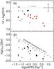 |
Fig. 10 Metallicity a) and H2 depletion timescale b) as a function of specific SFR. Symbols are as in Fig. 9, but red points in a) indicate BCDs with higher gas fractions (MHI/ (MHI + M∗) > 0.5) BCDs. The dotted line in a) indicates solar metallicity, while the dashed line in b) shows the correlation found by Saintonge et al. (2011) for local star-forming disk galaxies of stellar masses M∗ ≳ 1010M⊙. |
In the above studies, however, most nearby dwarfs studied in detail are dIs, while BCDs are strongly underrepresented. Dwarf irregulars form stars at lower rates and their star formation histories are predominantly continuous, i.e., they are main sequence galaxies in the SFR−M∗ relation (e.g., Brinchmann et al. 2004; Noeske et al. 2007; Lee et al. 2011; Hunt et al. 2012). In contrast, BCDs show more extreme conditions (e.g., high ISM ionization and higherspecific SFR (sSFR); Hunt et al. 2012; Amorín et al. 2014a, 2015), thus having predominantly “bursty” star-formation histories (e.g., Martín-Manjón et al. 2012).Therefore, one can argue that part of the enhancement in the SFE of BCDs seen in the SK law is due to a more bursty SF history. In this line, previous studies that are based on FIR/sub-mm data have found that even using a higher CO-to-H2 conversion factor, the depletion timescales for molecular gas in some metal-poor star forming galaxies appear considerably shorter than for normal spirals (e.g., Israel 1997; Gardan et al. 2007; Gratier et al. 2010a,b).
Following the above reasoning, in Fig. 10 we investigate the relation between sSFR and both H2 depletion timescale and metallicity. On average, we find that high sSFR BCDs have lower metallicity (Fig. 10a). These high sSFR galaxies also show higher Hi gas mass fractions (red circles). Despite the large scatter, Fig. 10b suggests that BCDs with higher sSFR tend to have shorter τH2. A similar trend was presented by Saintonge et al. (2011, dashed line in Fig. 106 for more massive (M⋆ ≳ 10 M⊙) star-forming galaxies of the COLDGASS survey (Saintonge et al. 2011). In their sample, however, the sSFR is not correlated with metallicity. In Fig. 10b, our BCDs follow the slope of the relation for the COLDGASS sample, but they appear shifted to significantly shorter H2 depletion timescales for a given sSFR. These results are consistent with Leroy et al. (2013), who found that the eight less massive (<1010M⊙) galaxies in the HERACLES survey are systematically offset to larger τH2 for a given sSFR when compared to more massive galaxies.
Taken together, results from Figs. 9 and 10 are mutually consistent and allow us to conclude that less massive and more metal-poor gas-rich galaxies, which form stars at higher rates, are those with shorter H2 depletion timescales.
In the next section, we use theses findings to derive a CO-to-H2 conversion factor for BCDs, derive their H2 masses, and revisit the scaling relations between star formation, gas content, and metallicity.
7. Deriving a metallicity-dependent CO-to-H2 conversion factor for starbursting dwarfs
To derive an expression for a metallicity-dependent CO-to-H2 conversion factor, we use αCO,Z/αCO,MW ≡ τH2 × ΣSFR/ ΣH2, where τH2 is the expected galaxy-averaged H2 depletion timescale for which metallicity effects have been accounted. Using the relation found between ΣSFR/ ΣH2 and metallicity (Table 5), we arrive at the following expression:  (2)with a 1σ dispersion of 0.32 in the slope. Possible systematic uncertainties not included in Eq. (2), e.g., those propagated from the derivation of integrated properties and driven by the numerous assumptions made, are likely larger and have not been taken into account.
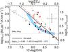 |
Fig. 11 CO-to-H2 conversion factor, αCO, as a function of the gas-phase metallicity. The right y-axis shows the ratio between the metallicity-dependent conversion factor and the constant value for the Milky Way (horizontal dashed line). A dotted vertical line indicates the solar metallicity. Black and gray dots show subsample I and subsample II BCDs, respectively, while the black solid line shows their best linear fit, indicated in the legend. Error bars indicate typical uncertainties for our sample. Red dots indicate dust-based measurements for five BCDs in our sample with Herschel data (see text). Triangles show dust-based measurements for Local Volume galaxies from Leroy et al. (2011), open circles show lower limits for the extremely metal-poor BCDs SBS 0335-052 and I Zw 18 (Hunt et al. 2014), and the magenta cross corresponds to the dIrr galaxy WLM from Elmegreen et al. (2013). Blue, red, and orange dashed lines show best fits for the same relation given by Arimoto et al. (1996), Genzel et al. (2012), and Schruba et al. (2012), respectively. The model prediction of Wolfire et al. (2010) (as presented in Sandstrom et al. 2013) is shown as a light blue band. |
To derive a suitable value for the CO-to-H2 conversion factor, Eq. (2) still requires the use of an appropriate value for τH2. One possibility would be to derive H2 masses from dust masses by assuming a dust-to-gas (D/G) ratio, and then computing τH2. Especially in compact low-metallicity galaxies, this approach is, however, not free of large uncertainties, which are mostly driven by variations in the D/G ratio with the ISM density (Schruba et al. 2012), uncertainties in its calibration at different metallicities, and variations with the SF history of each galaxy (Cormier et al. 2014; Rémy-Ruyer et al. 2014; see also Bolatto et al. 2013). In our case, only ~20% of the BCD sample have Herschel observations reported so far (see Rémy-Ruyer et al. 2015), thus precluding a complete analysis based on the dust masses.
Another method recently used in the literature relies on the underlying assumption of a constant SFE (τH2) for all galaxies (e.g., Schruba et al. 2012; Genzel et al. 2012; see also McQuinn et al. 2012). This method has been motivated by the relatively constant SFE found in nearby disk galaxies (Bigiel et al. 2008, 2011; Leroy et al. 2008) and recent theoretical works (e.g., Krumholz et al. 2011) that show that the H2 gas depletion timescale is uniform and does not depend on metallicity. However, in view of Fig. 10, the hypothesis of a constant τH2 does not appear particularly appropriate for dwarf galaxies with predominately bursty SF histories.
Therefore, in this work we choose an alternative method for obtaining τH2 for each galaxy, assuming that this quantity should follow a well established linear relation with sSFR at all masses (e.g., Saintonge et al. 2011; Boselli et al. 2014; Huang & Kauffmann 2014). In particular, we use the relation derived by Saintonge et al. (2011) for star-forming galaxies of stellar masses M ≳ 1010M⊙ in the COLDGAS survey (Fig. 10), under the reasonable assumption that it extends to lower stellar masses (dashed line in Fig. 10). Thus, we obtain the expected τH2 from the ratio between the observed τH2 computed via the galactic CO-to-H2 conversion factor and the linear fit of Saintonge et al. (2011) for a given sSFR (Fig. 10b). Finally, we use this value and Eq. (2) and derive αCO(Z) for each galaxy.
In Fig. 11, we show the derived αCO as a function of metallicity. Despite the large scatter log αCO appear to scale linearly with metallicity, meaning that αCO∝ (Z/Z⊙)-1.5. This relation is in qualitative agreement with previous determinations, dust-based measurements, and recent model predictions, as we discuss below. Figure 11 suggests that, in vigorously star-forming dwarfs, the fraction of H2 traced by CO decreases a factor of about 40 from Z ~ Z⊙ to Z ~ 0.1 Z⊙, leading to a strong underestimation of the H2 mass in metal-poor systems when a Galactic αCO,MW is considered.
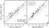 |
Fig. 12 Star-formation rate surface density as a function of the expected H2 (left) and Hi+H2 (right) gas surface densities after adopting the derived metallicity-dependent CO-to-H2 conversion factor αCO,Z from Eq. (2) (Fig. 11). Lines and symbols are as in Fig. 8. |
In Figure 11, we included dust-based αCO measurements for the five BCDs in the sample with Herschel data (red dots). We used the dust masses compiled by Rémy-Ruyer et al. (2014, 2015) to derive the H2 masses following Cormier et al. (2014) and assuming the metallicity dependent D/G ratio of Rémy-Ruyer et al. (2015). The resulting dust-based MH2 and αCO,dust are a factor of ~1.5–30 higher than those derived using the Galactic αCO,MW. Within the errors (larger than a factor of 2), the dust-based measurements are consistent with those based on our method and with the best-fit relation (αCO,Z∝ (Z/Z⊙)-1.5), as shown in Fig. 11.
Similarly, our relation is broadly consistent with independent measurements of αCO, based on different methods for other nearby star-forming galaxies of sub-solar metallicity. For example, our data are consistent with values based on dust-modelling along the lines of sight from IR emission of five Local Group galaxies (see Fig. 11) by Leroy et al. (2011). Also, our power law index is ~50% higher than the one found by Arimoto et al. (1996), based on the virial masses of giant molecular clouds of the Milky Way and eight additional nearby spirals and dIs (blue dashed line). Our index, instead, is in agreement within the uncertainties with an index of ~1.6 derived by Genzel et al. (2012) for more massive star-forming galaxies at z ≤ 1 assuming that galaxies follow a universal SK law of n = 1.3 (red line in Fig. 11). Also Schruba et al. (2012) studied the αCO−Z relation for five HERACLES dwarf galaxies, assuming a constant value for τH2 = 1.8 Gyr. They found a power law index ≳2 (orange line in Fig. 11), which is significantly higher than ours.
Although the above results are qualitatively similar, quantitative differences are likely associated with the underlying assumptions behind each method, biases towards a certain galaxy class, and different dynamic ranges in metallicity, as well as uncertainties in its determination. In particular, the method based on a constant τH2 has the caveat that it might mask out any true variation of the SFE with sSFR at different metallicities.
Finally, we find that in spite of the different parametrization (power law vs. exponential) our αCO−Z relation is broadly consistent with model predictions7 of Wolfire et al. (2010) from solar to ~10% solar metallicities.
7.1. Revisiting the molecular content and star-formation laws
We use now the metallicity dependent CO-to-H2 conversion factor αCO,Z that was obtained in the previous section to recompute H2 masses and surface densities8. Using these quantities, we revisit different scaling relations that have been presented before (Figs. 8–10). Thus, in Fig. 12 we show the corrected position of BCDs in the SK-law, while in Fig. 14 we show the same quantities as in Fig. 9, but using αCO,Z. In Figs. 14c, d, we included the predictions of models by Krumholz et al. (2011, magenta and blue lines, respectively).
We find that the use of a metallicity-dependent CO-to-H2 conversion factor αCO(Z) from Eq. (2) removes only part of the large offset position that is observed for BCDs in the SK law for molecular and total (Hi+H2) gas that is followed by more massive starbursts and late-type galaxies. In particular, our results suggest that BCDs have shorter depletion timescales compared to normal late-type disks. Starbursting dwarfs with larger gas fractions, low metallicity and higher SSFRs still show shorter depletion timescales for the molecular phase. This conclusion arises from Figs. 13 and 14c. While some galaxies seem to agree with Krumholz et al. (2011) models (magenta lines) that predict a constant SFE(H2) with metallicity, some metal-poor dwarfs show a significantly increased efficiency. We note, however, that this result is in qualitative agreement with other model predictions (Pelupessy & Papadopoulos 2009; Dib 2011), which predict pronounced variations of τH2 with metallicity during brief periods of intense star formation. BCDs with shorter molecular depletion timescales tend to show lower molecular fractions and higher sSFR, as shown in Figs. 14a, b and 13. The depletion timescales for molecular plus atomic gas, instead, do not appear to be a strong function of metallicity, in qualitative agreement with the models of Krumholz et al. (2011; blue lines).
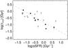 |
Fig. 13 Molecular depletion timescale, as derived using αCO,Z from Eq. (2) (see text), as a function of the specific SFR. Symbols and lines are as in Fig. 10b. |
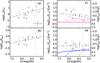 |
Fig. 14 Same as Fig. 9, but using the molecular masses derived using αCO(Z) from Eq. (2) (see text). Black and gray dashed lines show linear best fits tosubsample I andsubsample II. Solid, dotted and dashed magenta (blue) lines in panel c), d) show model predictions by Krumholz et al. (2011) for different values of Σgas (80, 20 and 5 M⊙ pc-2, respectively). |
8. Summary and conclusions
We have studied the molecular content of a large and representative sample of 21 blue compact dwarf galaxies that was selected from a series of previous works. To this end, we have conducted new CO (1–0) and (2–1) single-dish observations of a sub-sample of ten BCDs using the IRAM-30m telescope, further supplemented with similar data from the literature for the remaining 11 BCDs. Our CO observations have yielded seven (>3σ) detections, one marginal (~3σ) detection in CO(2–1), and two non-detections. For two BCDs (III Zw 107 and Mrk 401) CO emission has been detected for the first time. The derived CO luminosities, in combination with an extensive ancillary data set, have been used to study their relation to several galaxy-averaged properties, including SFR tracers, stellar and Hi masses, sizes, and metallicity, as well as their impact on star-formation laws. We summarize our conclusions in the following:
-
The amount of molecular mass that is traced by CO in BCDs scales with both stellar and Hi gas masses and all SFR tracers that have been studied so far, in good agreement with previous findings for dwarf galaxies in general. Our results suggest that, over galaxy-wide scales, more massive and luminous BCDs – i.e., those with strong and extended star-forming regions – are favoured for CO detections. However, CO luminosity is a strong function of the gas-phase metallicity, which puts the most stringent constraint (Z ≳ 0.3 Z⊙) on the CO detectability in BCDs.
-
In the context of the Schmidt-Kennicutt law, BCDs show larger SFR surface densities, compared with other late-type galaxies. Thus, they appear systematically offset to lower H2 and H2 +Hi depletion timescales from the general trend that is followed by dwarfs irregulars, spiral discs, and more massive and dusty starbursts. We find a strong correlation between the BCD metallicity and both the molecular gas fraction and the molecular gas-depletion timescale; more metal-poor BCDs show lower molecular gas fractions and shorter depletion timescales than more metal-rich BCDs. However, for the total (molecular plus atomic) gas-depletion timescale the metallicity dependence becomes significantly reduced. Overall, we find that more metal-poor, gas-rich, and high sSFR BCDs are those with shorter H2 depletion timescales, under the assumption of a constant (Milky Way) CO-to-H2 conversion factor.
-
We discuss the above results in the context of the CO-to-H2 conversion factor αCO. We have derived a metallicity-dependent CO-to-H2 conversion factor using the empirical relations found between τH2 and both metallicity and specific SFR. The result is log (αCO,Z) = 0.7−1.5 × (12 + log (O / H)−8.7) (or αCO,Z ∝ (Z/Z⊙)− y, with y = 1.5 ± 0.3). This power law is in qualitative agreement with previous determinations that are based on dust-based H2 masses and the model predictions of Wolfire et al. (2010). Our power-law index is, however, higher than values that are based on virial masses of molecular clouds, and slightly lower than values found, assuming a universal τH2 (e.g., Schruba et al. 2012; Genzel et al. 2012). This result suggest that, in vigorously star-forming dwarfs, the fraction of H2 traced by CO decreases by a factor of about 40 from Z ~ Z⊙ to Z ~ 0.1 Z⊙, leading to a strong underestimation of the H2 mass in metal-poor systems when a Galactic XCO,MW is considered. This supports previous work that suggests that, in metal-poor and highly ionized environments – such as those in high sSFR BCDs – massive star formation is found in increasingly CO-free molecular clouds. According to models (e.g., Wolfire et al. 2010) this is likely because of a rapid decrease in dust shielding and, consequently, strong UV photodissociation (see also Bolatto et al. 2013).
-
The observed relations between H2, SFR, and metallicity change when adopting the metallicity-dependent αCO, alleviating the offset position of BCDs in the SK laws, but not removing it completely. Our analysis suggest that starbursting dwarfs have shorter depletion gas timescales when compared to normal late-type discs, even accounting for the molecular gas not traced by CO emission in metal-poor environments. Thus, τmol does not appears constant with metallicity but shows a small increase with metallicity, which is mainly driven by galaxies with higher sSFR and gas fraction. While this produces some tension with some models (Krumholz et al. 2011), it appears to agree qualitatively with model predictions for brief and intense episodes of star formation (Pelupessy & Papadopoulos 2009; Dib et al. 2011). While the revised relations between the molecular to atomic gas surface density ratio and molecular fraction with metallicity show a shallower slope, the total (H2 +Hi) gas depletion timescale tends to become nearly constant with metallicity, in qualitative agreement with model predictions by Krumholz et al. (2011).
We note that in the process of refereeing the present paper, a work by Hunt et al. (2015), which tackles similar goals, has just been published. Their results on the CO emission of eight low-metallicity dwarf galaxies are certainly complementary to the work presented here, and their conclusions on the molecular depletion timescales of these galaxies appear in good agreement with ours.
Further insights on the above conclusions would benefit from future studies that use larger samples of star-forming dwarfs, for which large and homogeneous multiwavelength datasets are currently available (e.g., the AVOCADO project, Sánchez-Janssen et al. 2013).
Being rare in the Local Universe, BCDs are one of the best local analogues of low-mass star-forming galaxies at high redshift. The strong limitations found on the use of CO as a suitable tracer of the molecular gas that is involved in the onset of starburst activity in nearby BCDs clearly underline the strong challenge that exists when tracing the molecular content of chemically unevolved galaxies in the early Universe, even using the unprecedented sensitivity of ALMA.
HPBW [arcsec] = 2460/ν [GHz], where ν is the observed frequency.
The CLASS software package is part of the GILDAS software, and can be downloaded from the IRAM website: http://www.iram.fr/IRAMFR/GILDAS/
In all cases the K magnitudes are those obtained with the largest aperture (~4 times the J-band effective radius).
Based on the NED: http://ned.ipac.caltech.edu/
The relation given by Saintonge et al. (2011) does not include Helium in ΣH2, so we have corrected their relation upwards to be consistent with our measurements.
We use models from Wolfire et al. (2010) normalized to αCO = 4.4 M⊙ pc-2 (K km s-1)-1 at solar metallicity, as presented in Sandstrom et al. 2013, see also Leroy et al. (2013). The models assume a fixed gas mass surface-density for molecular clouds and a linear scaling between the dust-to-gas ratio and metallicity.
To distinguish these quantities from those derived through a Galactic CO-to-H2 conversion factor, we adopted a different subscript (mol), so Mmol and Σmol.
Acknowledgments
The authors would like to thank the referee, J. Braine, for his helpful reports which significantly contributed to improving this manuscript. We are grateful to the staff of the IRAM 30m telescope for their support during the observations, and in particular to Sergio Martin. We thank U. Lisenfeld, J. M. Vílchez, P. Papaderos and S. Dib for helpful comments on the analysis. A significant part of this work has been presented in the Ph.D. Thesis of R.A. (Universidad de La Laguna, Spain, October 2008). This work has been partially funded by the Spanish DGCyT, grants AYA2010-21887-C04-01, AYA2010-21887-C04-04, AYA2013-47742-C4-2-P, AYA2012-32295, AYA2013-43188-P, and FIS2012-32096. This research was partially funded by the Spanish MEC under the Consolider-Ingenio 2010 Program grant CSD2006-00070: First Science with the GTC (http://www.iac.es/consolider-ingenio-gtc/). R.A. also acknowledges the contribution of the FP7 SPACE project, ASTRODEEP, (Ref.No: 312725), supported by the European Commission. This research has made use of the NASA/IPAC Extragalactic Database (NED), which is operated by the Jet Propulsion Laboratory, California Institute of Technology, under contract with the National Aeronautics and Space Administration.
References
- Albrecht, M., Chini, R., Krügel, E., Müller, S. A. H., & Lemke, R. 2004, A&A, 414, 141 [NASA ADS] [CrossRef] [EDP Sciences] [Google Scholar]
- Allen de Prieto, C., Lambert, D. L., & Asplund, M. 2001, ApJ, 556, L63 [NASA ADS] [CrossRef] [Google Scholar]
- Amorín, R. O. 2010, PASP, 122, 495 [NASA ADS] [CrossRef] [Google Scholar]
- Amorín, R. O., Muñoz-Tuñón, C., Aguerri, J. A. L., Cairós, L. M., & Caon, N. 2007, A&A, 467, 541 [NASA ADS] [CrossRef] [EDP Sciences] [Google Scholar]
- Amorín, R. O., Pérez-Montero, E., & Vílchez, J. M. 2010, ApJ, 715, L128 [NASA ADS] [CrossRef] [Google Scholar]
- Amorín, R. 2008, Ph.D. Thesis, Universidad de La Laguna, Spain [Google Scholar]
- Amorín, R., Aguerri, J. A. L., Muñoz-Tuñón, C., & Cairós, L. M. 2009, A&A, 501, 75 [NASA ADS] [CrossRef] [EDP Sciences] [Google Scholar]
- Amorín, R., Pérez-Montero, E., Vílchez, J. M., & Papaderos, P. 2012, ApJ, 749, 185 [NASA ADS] [CrossRef] [Google Scholar]
- Amorín, R., Sommariva, V., Castellano, M., et al. 2014a, A&A, 568, L8 [NASA ADS] [CrossRef] [EDP Sciences] [Google Scholar]
- Amorín, R., Grazian, A., Castellano, M., et al. 2014b, ApJ, 788, L4 [NASA ADS] [CrossRef] [Google Scholar]
- Amorín, R., Pérez-Montero, E., Contini, T., et al. 2015, A&A, 578, A105 [NASA ADS] [CrossRef] [EDP Sciences] [Google Scholar]
- Arimoto, N., Sofue, Y., & Tsujimoto, T. 1996, PASJ, 48, 275 [NASA ADS] [CrossRef] [Google Scholar]
- Barone, L. T., Heithausen, A., Hüttemeister, S., Fritz, T., & Klein, U. 2000, MNRAS, 317, 649 [NASA ADS] [CrossRef] [Google Scholar]
- Bekki, K. 2008, MNRAS, 388, L10 [Google Scholar]
- Bell, E. F., & de Jong, R. S. 2001, ApJ, 550, 212 [NASA ADS] [CrossRef] [Google Scholar]
- Bigiel, F., Leroy, A., Walter, F., et al. 2008, AJ, 136, 2846 [NASA ADS] [CrossRef] [Google Scholar]
- Bigiel, F., Leroy, A. K., Walter, F., et al. 2011, ApJ, 730, L13 [NASA ADS] [CrossRef] [Google Scholar]
- Bolatto, A. D., Leroy, A. K., Jameson, K., et al. 2011, ApJ, 741, 12 [NASA ADS] [CrossRef] [Google Scholar]
- Bolatto, A. D., Wolfire, M., & Leroy, A. K. 2013, ARA&A, 51, 207 [Google Scholar]
- Boselli, A., Cortese, L., Boquien, M., et al. 2014, A&A, 564, A66 [NASA ADS] [CrossRef] [EDP Sciences] [Google Scholar]
- Brinchmann, J., Charlot, S., White, S. D. M., et al. 2004, MNRAS, 351, 1151 [NASA ADS] [CrossRef] [Google Scholar]
- Brosch, N., Almoznino, E., & Heller, A. B. 2004, MNRAS, 349, 357 [NASA ADS] [CrossRef] [Google Scholar]
- Buat, V., Iglesias-Páramo, J., Seibert, M., et al. 2005, ApJ, 619, L51 [NASA ADS] [CrossRef] [Google Scholar]
- Buisson, G., Desbats, L., Duvert, G., et al. 1997, Continuum and Line Analysis Single-dish Software, Observatoire de Grenoble and IRAM [Google Scholar]
- Campos-Aguilar, A., Moles, M., & Masegosa, J. 1993, AJ, 106, 1784 [NASA ADS] [CrossRef] [Google Scholar]
- Cairós, L. M., Vílchez, J. M., González Pérez, J. N., Iglesias-Páramo, J., & Caon, N. 2001a, ApJS, 133, 321 [NASA ADS] [CrossRef] [Google Scholar]
- Cairós, L. M., Caon, N., Vílchez, J. M., González-Pérez, J. N., & Muñoz-Tuñón, C. 2001b, ApJS, 136, 393 [NASA ADS] [CrossRef] [Google Scholar]
- Cairós, L. M., Caon, N., Papaderos, P., et al. 2003, ApJ, 593, 312 [NASA ADS] [CrossRef] [Google Scholar]
- Cairós, L. M., Caon, N., García-Lorenzo, B., et al. 2007, ApJ, 669, 251 [NASA ADS] [CrossRef] [Google Scholar]
- Caon, N., Cairós, L. M., Aguerri, J. A. L., & Muñoz-Tuñón, C. 2005, ApJS, 157, 218 [NASA ADS] [CrossRef] [Google Scholar]
- Cardelli, J. A., Clayton, G. C., & Mathis, J. S. 1989, ApJ, 345, 245 [NASA ADS] [CrossRef] [Google Scholar]
- Condon, J. J., Cotton, W. D., Greisen, E. W., et al. 1998, AJ, 115, 1693 [NASA ADS] [CrossRef] [Google Scholar]
- Cormier, D., Madden, S. C., Lebouteiller, V., et al. 2014, A&A, 564, A121 [NASA ADS] [CrossRef] [EDP Sciences] [Google Scholar]
- Dame, T. M., Hartmann, D., & Thaddeus, P. 2001, ApJ, 547, 792 [NASA ADS] [CrossRef] [Google Scholar]
- Dale, D. A., & Helou, G. 2002, ApJ, 576, 159 [NASA ADS] [CrossRef] [Google Scholar]
- Dale, D. A., Helou, G., Neugebauer, G., et al. 2001, AJ, 122, 1736 [NASA ADS] [CrossRef] [Google Scholar]
- Davies, J. I., & Phillipps, S. 1988, MNRAS, 233, 553 [NASA ADS] [CrossRef] [Google Scholar]
- de Barros, S., Vanzella, E., Amorín, R., et al. 2016, A&A, 585, A51 [NASA ADS] [CrossRef] [EDP Sciences] [Google Scholar]
- Dib, S. 2011, ApJ, 737, L20 [NASA ADS] [CrossRef] [Google Scholar]
- Dib, S., Piau, L., Mohanty, S., & Braine, J. 2011, MNRAS, 415, 3439 [NASA ADS] [CrossRef] [Google Scholar]
- Draine, B. T., Dale, D. A., Bendo, G., et al. 2007, ApJ, 663, 866 [NASA ADS] [CrossRef] [Google Scholar]
- Elfhag, T., Booth, R. S., Hoeglund, B., Johansson, L. E. B., & Sandqvist, A. 1996, A&AS, 115, 439 [NASA ADS] [Google Scholar]
- Elmegreen, B. G., Zhang, H.-X., & Hunter, D. A. 2012, ApJ, 747, 105 [NASA ADS] [CrossRef] [Google Scholar]
- Elmegreen, B. G., Rubio, M., Hunter, D. A., et al. 2013, Nature, 495, 487 [NASA ADS] [CrossRef] [Google Scholar]
- Ekta, B., & Chengalur, J. N. 2010, MNRAS, 403, 295 [NASA ADS] [CrossRef] [Google Scholar]
- Filho, M. E., Winkel, B., Sánchez Almeida, J., et al. 2013, A&A, 558, A18 [NASA ADS] [CrossRef] [EDP Sciences] [Google Scholar]
- Frayer, D. T., Seaquist, E. R., Thuan, T. X., & Sievers, A. 1998, ApJ, 503, 231 [NASA ADS] [CrossRef] [Google Scholar]
- Fumagalli, M., Krumholz, M. R., & Hunt, L. K. 2010, ApJ, 722, 919 [NASA ADS] [CrossRef] [Google Scholar]
- García-Lorenzo, B., Cairós, L. M., Caon, N., Monreal-Ibero, A., & Kehrig, C. 2008, ApJ, 677, 201 [NASA ADS] [CrossRef] [Google Scholar]
- Gardan, E., Braine, J., Schuster, K. F., Brouillet, N., & Sievers, A. 2007, A&A, 473, 91 [NASA ADS] [CrossRef] [EDP Sciences] [Google Scholar]
- Garland, C. A., Williams, J. P., Pisano, D. J., et al. 2005, ApJ, 624, 714 [NASA ADS] [CrossRef] [Google Scholar]
- Genzel, R., Tacconi, L. J., Combes, F., et al. 2012, ApJ, 746, 69 [NASA ADS] [CrossRef] [Google Scholar]
- Gerola, H., Seiden, P. E., & Schulman, L. S. 1980, ApJ, 242, 517 [NASA ADS] [CrossRef] [Google Scholar]
- Gil de Paz, A., & Madore, B. F. 2005, ApJS, 156, 345 [NASA ADS] [CrossRef] [EDP Sciences] [Google Scholar]
- Gil de Paz, A., Madore, B. F., & Pevunova, O. 2003, ApJS, 147, 29 [NASA ADS] [CrossRef] [Google Scholar]
- Glover, S. C. O., & Clark, P. C. 2012, MNRAS, 426, 377 [NASA ADS] [CrossRef] [Google Scholar]
- Glover, S. C. O., & Mac Low, M.-M. 2011, MNRAS, 412, 337 [NASA ADS] [CrossRef] [MathSciNet] [Google Scholar]
- Gnedin, N. Y., & Kravtsov, A. V. 2010, ApJ, 714, 287 [NASA ADS] [CrossRef] [Google Scholar]
- Gordon, D., & Gottesman, S. T. 1981, AJ, 86, 161 [NASA ADS] [CrossRef] [Google Scholar]
- Gratier, P., Braine, J., Rodriguez-Fernandez, N. J., et al. 2010a, A&A, 522, A3 [NASA ADS] [CrossRef] [EDP Sciences] [Google Scholar]
- Gratier, P., Braine, J., Rodriguez-Fernandez, N. J., et al. 2010b, A&A, 512, A68 [NASA ADS] [CrossRef] [EDP Sciences] [Google Scholar]
- Helou, G., Khan, I. R., Malek, L., & Boehmer, L. 1988, ApJS, 68, 151 [NASA ADS] [CrossRef] [Google Scholar]
- Huang, M.-L., & Kauffmann, G. 2014, MNRAS, 443, 1329 [NASA ADS] [CrossRef] [Google Scholar]
- Hunt, L., Magrini, L., Galli, D., et al. 2012, MNRAS, 427, 906 [NASA ADS] [CrossRef] [Google Scholar]
- Hunt, L. K., Testi, L., Casasola, V., et al. 2014, A&A, 561, A49 [NASA ADS] [CrossRef] [EDP Sciences] [Google Scholar]
- Hunt, L. K., García-Burillo, S., Casasola, V., et al. 2015, A&A, 583, A114 [NASA ADS] [CrossRef] [EDP Sciences] [Google Scholar]
- Hunter, D. A., & Elmegreen, B. G. 2004, AJ, 128, 2170 [NASA ADS] [CrossRef] [Google Scholar]
- Hunter, D. A., & Elmegreen, B. G. 2006, ApJS, 162, 49 [NASA ADS] [CrossRef] [Google Scholar]
- Israel, F. P. 1997, A&A, 328, 471 [NASA ADS] [Google Scholar]
- Israel, F. P. 2005, A&A, 438, 855 [NASA ADS] [CrossRef] [EDP Sciences] [Google Scholar]
- Izotov, Y. I., Papaderos, P., Guseva, N. G., Fricke, K. J., & Thuan, T. X. 2006, A&A, 454, 137 [NASA ADS] [CrossRef] [EDP Sciences] [Google Scholar]
- Jarrett, T. H., Chester, T., Cutri, R., et al. 2000, AJ, 119, 2498 [NASA ADS] [CrossRef] [Google Scholar]
- Kennicutt, R. C., Jr. 1998, ApJ, 498, 541 [NASA ADS] [CrossRef] [Google Scholar]
- Kennicutt, R. C., Jr., Hao, C. N., Calzetti, D., et al. 2009, ApJ, 703, 1672 [NASA ADS] [CrossRef] [Google Scholar]
- Kennicutt, R. C., & Evans, N. J. 2012, ARA&A, 50, 531 [NASA ADS] [CrossRef] [Google Scholar]
- Kniazev, A. Y., Pustilnik, S. A., Grebel, E. K., Lee, H., & Pramskij, A. G. 2004, ApJS, 153, 429 [NASA ADS] [CrossRef] [Google Scholar]
- Koulouridis, E., Plionis, M., Chávez, R., et al. 2013, A&A, 554, A13 [NASA ADS] [CrossRef] [EDP Sciences] [Google Scholar]
- Krumholz, M. R., McKee, C. F., & Tumlinson, J. 2009, ApJ, 699, 850 [NASA ADS] [CrossRef] [Google Scholar]
- Krumholz, M. R., Leroy, A. K., & McKee, C. F. 2011, ApJ, 731, 25 [NASA ADS] [CrossRef] [Google Scholar]
- Kunth, D., & Östlin, G. 2000, A&ARv, 10, 1 [NASA ADS] [CrossRef] [Google Scholar]
- Lagos, P., Telles, E., & Melnick, J. 2007, A&A, 476, 89 [NASA ADS] [CrossRef] [EDP Sciences] [Google Scholar]
- Lee, J. C., Gil de Paz, A., Kennicutt, R. C., Jr., et al. 2011, ApJS, 192, 6 [NASA ADS] [CrossRef] [Google Scholar]
- Leon, S., Combes, F., & Menon, T. K. 1998, A&A, 330, 37 [NASA ADS] [Google Scholar]
- Lelli, F., Fraternali, F., & Verheijen, M. 2014a, A&A, 563, A27 [NASA ADS] [CrossRef] [EDP Sciences] [Google Scholar]
- Lelli, F., Verheijen, M., & Fraternali, F. 2014b, A&A, 566, A71 [NASA ADS] [CrossRef] [EDP Sciences] [Google Scholar]
- Leroy, A., Bolatto, A. D., Simon, J. D., & Blitz, L. 2005, ApJ, 625, 763 [NASA ADS] [CrossRef] [Google Scholar]
- Leroy, A., Bolatto, A., Walter, F., & Blitz, L. 2006, ApJ, 643, 825 [NASA ADS] [CrossRef] [Google Scholar]
- Leroy, A., Cannon, J., Walter, F., Bolatto, A., & Weiss, A. 2007, ApJ, 663, 990 [NASA ADS] [CrossRef] [MathSciNet] [Google Scholar]
- Leroy, A. K., Walter, F., Brinks, E., et al. 2008, AJ, 136, 2782 [NASA ADS] [CrossRef] [Google Scholar]
- Leroy, A. K., Bolatto, A., Gordon, K., et al. 2011, ApJ, 737, 12 [NASA ADS] [CrossRef] [Google Scholar]
- Leroy, A. K., Walter, F., Sandstrom, K., et al. 2013, AJ, 146, 19 [NASA ADS] [CrossRef] [Google Scholar]
- López-Sánchez, Á. R., & Esteban, C. 2010, A&A, 517, A85 [NASA ADS] [CrossRef] [EDP Sciences] [Google Scholar]
- López-Sánchez, Á. R., Koribalski, B. S., van Eymeren, J., et al. 2012, MNRAS, 419, 1051 [NASA ADS] [CrossRef] [Google Scholar]
- Mac Low, M.-M., & Ferrara, A. 1999, ApJ, 513, 142 [NASA ADS] [CrossRef] [Google Scholar]
- Martin, D. C., Christopher, F., James, S., et al. 2005, ApJ, 619, L1 [Google Scholar]
- Martín-Manjón, M. L., Mollá, M., Díaz, A. I., & Terlevich, R. 2012, MNRAS, 420, 1294 [NASA ADS] [CrossRef] [Google Scholar]
- Maseda, M. V., van der Wel, A., Rix, H.-W., et al. 2014, ApJ, 791, 17 [CrossRef] [Google Scholar]
- McQuinn, K. B. W., Skillman, E. D., Dalcanton, J. J., et al. 2012, ApJ, 751, 127 [NASA ADS] [CrossRef] [Google Scholar]
- Micheva, G., Östlin, G., Bergvall, N., et al. 2013, MNRAS, 431, 102 [NASA ADS] [CrossRef] [Google Scholar]
- Morales-Luis, A. B., Sánchez Almeida, J., Aguerri, J. A. L., & Muñoz-Tuñón, C. 2011, ApJ, 743, 77 [NASA ADS] [CrossRef] [Google Scholar]
- Morrissey, P., chiminovich, D., Barlow, T. A., et al. 2005, ApJ, 619, L7 [NASA ADS] [CrossRef] [Google Scholar]
- Moshir, M., Kopan, G., Conrow, T., et al. 1990, IRAS Faint Source Catalogue, BAAS, 22, 1325 [NASA ADS] [Google Scholar]
- Narayanan, D., Krumholz, M. R., Ostriker, E. C., & Hernquist, L. 2012, MNRAS, 421, 3127 [NASA ADS] [CrossRef] [Google Scholar]
- Noeske, K. G., Iglesias-Páramo, J., Vílchez, J. M., Papaderos, P., & Fricke, K. J. 2001, A&A, 371, 806 [NASA ADS] [CrossRef] [EDP Sciences] [Google Scholar]
- Noeske, K. G., Papaderos, P., Cairós, L. M., & Fricke, K. J. 2003, A&A, 410, 481 [NASA ADS] [CrossRef] [EDP Sciences] [Google Scholar]
- Noeske, K. G., Papaderos, P., Cairós, L. M., & Fricke, K. J. 2005, A&A, 429, 115 [NASA ADS] [CrossRef] [EDP Sciences] [Google Scholar]
- Noeske, K. G., Weiner, B. J., Faber, S. M., et al. 2007, ApJ, 660, L43 [Google Scholar]
- Papaderos, P., Loose, H.-H., Thuan, T. X., & Fricke, K. J. 1996a, A&AS, 120, 207 [NASA ADS] [CrossRef] [EDP Sciences] [Google Scholar]
- Papaderos, P., Loose, H.-H., Fricke, K. J., & Thuan, T. X. 1996b, A&A, 314, 59 [NASA ADS] [Google Scholar]
- Papaderos, P., Guseva, N. G., Izotov, Y. I., et al. 2006, A&A, 457, 45 [NASA ADS] [CrossRef] [EDP Sciences] [Google Scholar]
- Papaderos, P., Guseva, N. G., Izotov, Y. I., & Fricke, K. J. 2008, A&A, 491, 113 [NASA ADS] [CrossRef] [EDP Sciences] [Google Scholar]
- Pelupessy, F. I., & Papadopoulos, P. P. 2009, ApJ, 707, 954 [NASA ADS] [CrossRef] [Google Scholar]
- Pérez-Montero, E., & Díaz, A. I. 2003, MNRAS, 346, 105 [NASA ADS] [CrossRef] [Google Scholar]
- Pérez-Montero, E., & Contini, T. 2009, MNRAS, 398, 949 [NASA ADS] [CrossRef] [Google Scholar]
- Press, W. H., Teukolsky, S. A., Vetterling, W. T., & Flannery, B. P. 1992 Numerical Computing, 2nd ed. (Cambridge: University Press) [Google Scholar]
- Pustilnik, S. A., Kniazev, A. Y., Lipovetsky, V. A., & Ugryumov, A. V. 2001, A&A, 373, 24 [NASA ADS] [CrossRef] [EDP Sciences] [Google Scholar]
- Recchi, S., & Hensler, G. 2013, A&A, 551, A41 [NASA ADS] [CrossRef] [EDP Sciences] [Google Scholar]
- Rémy-Ruyer, A., Madden, S. C., Galliano, F., et al. 2014, A&A, 563, A31 [NASA ADS] [CrossRef] [EDP Sciences] [Google Scholar]
- Rémy-Ruyer, A., Madden, S. C., Galliano, F., et al. 2015, A&A, 582, A121 [NASA ADS] [CrossRef] [EDP Sciences] [Google Scholar]
- Rubio, M., Lequeux, J., & Boulanger, F. 1993, A&A, 271, 9 [NASA ADS] [Google Scholar]
- Rubio, M., Elmegreen, B. G., Hunter, D. A., et al. 2015, Nature, 525, 218 [NASA ADS] [CrossRef] [MathSciNet] [PubMed] [Google Scholar]
- Sánchez Almeida, J., Muñoz-Tuñón, C., Amorín, R., et al. 2008, ApJ, 685, 194 [NASA ADS] [CrossRef] [Google Scholar]
- Saintonge, A., Kauffmann, G., Kramer, C., et al. 2011a, MNRAS, 415, 32 [NASA ADS] [CrossRef] [Google Scholar]
- Saintonge, A., Kauffmann, G., Wang, J., et al. 2011b, MNRAS, 415, 61 [NASA ADS] [CrossRef] [Google Scholar]
- Sánchez Almeida, J., Muñoz-Tuñón, C., Elmegreen, D. M., Elmegreen, B. G., & Méndez-Abreu, J. 2013, ApJ, 767, 74 [NASA ADS] [CrossRef] [Google Scholar]
- Sánchez Almeida, J., Morales-Luis, A. B., Muñoz-Tuñón, C., et al. 2014, ApJ, 783, 45 [NASA ADS] [CrossRef] [Google Scholar]
- Sánchez Almeida, J., Elmegreen, B. G., Muñoz-Tuñón, C., et al. 2015, ApJ, 810, L15 [NASA ADS] [CrossRef] [Google Scholar]
- Sánchez-Janssen, R., Amorín, R., García-Vargas, M., et al. 2013, A&A, 554, A20 [NASA ADS] [CrossRef] [EDP Sciences] [Google Scholar]
- Sandstrom, K. M., Leroy, A. K., Walter, F., et al. 2013, ApJ, 777, 5 [NASA ADS] [CrossRef] [Google Scholar]
- Sargent, W. L. W., & Searle, L. 1970, ApJ, 162, L155 [NASA ADS] [CrossRef] [Google Scholar]
- Shi, F., Kong, X., & Cheng, F. Z. 2006, A&A, 453, 487 [NASA ADS] [CrossRef] [EDP Sciences] [Google Scholar]
- Shi, Y., Helou, G., Yan, L., et al. 2011, ApJ, 733, 87 [NASA ADS] [CrossRef] [Google Scholar]
- Schlegel, D. J., Finkbeiner, D. P., & Davis, M. 1998, ApJ, 500, 525 [NASA ADS] [CrossRef] [Google Scholar]
- Schmidt, M. 1959, ApJ, 129, 243 [NASA ADS] [CrossRef] [Google Scholar]
- Schruba, A., Leroy, A. K., Walter, F., et al. 2011, AJ, 142, 37 [NASA ADS] [CrossRef] [Google Scholar]
- Schruba, A., Leroy, A. K., Walter, F., et al. 2012, AJ, 143, 138 [NASA ADS] [CrossRef] [Google Scholar]
- Silich, S., & Tenorio-Tagle, G. 2001, ApJ, 552, 91 [NASA ADS] [CrossRef] [Google Scholar]
- Solomon, P. M., Downes, D., Radford, S. J. E., & Barrett, J. W. 1997, ApJ, 478, 144 [NASA ADS] [CrossRef] [Google Scholar]
- Strong, A. W., & Mattox, J. R. 1996, A&A, 308, L21 [NASA ADS] [Google Scholar]
- Taylor, C. L., Kobulnicky, H. A., & Skillman, E. D. 1998, AJ, 116, 2746 [NASA ADS] [CrossRef] [Google Scholar]
- Tacconi, L. J., & Young, J. S. 1987, ApJ, 322, 681 [NASA ADS] [CrossRef] [Google Scholar]
- Telles, E., & Terlevich, R. 1995, MNRAS, 275, 1 [NASA ADS] [CrossRef] [Google Scholar]
- Tenorio-Tagle, G., Muñoz-Tuñón, C., Pérez, E., Silich, S., & Telles, E. 2006, ApJ, 643, 186 [NASA ADS] [CrossRef] [Google Scholar]
- Terlevich, R., Melnick, J., Masegosa, J., Moles, M., & Copetti, M. V. F. 1991, A&AS, 91, 285 [NASA ADS] [Google Scholar]
- Thuan, T. X., & Martin, G. E. 1981, ApJ, 247, 823 [NASA ADS] [CrossRef] [Google Scholar]
- Vaduvescu, O., Richer, M. G., & McCall, M. L. 2006, AJ, 131, 1318 [NASA ADS] [CrossRef] [Google Scholar]
- van Zee, L., Skillman, E. D., & Salzer, J. J. 1998, AJ, 116, 1186 [NASA ADS] [CrossRef] [Google Scholar]
- van Zee, L., Salzer, J. J., & Skillman, E. D. 2001, AJ, 122, 121 [NASA ADS] [CrossRef] [Google Scholar]
- Verdes-Montenegro, L., Yun, M. S., Perea, J., del Olmo, A., & Ho, P. T. P. 1998, ApJ, 497, 89 [NASA ADS] [CrossRef] [Google Scholar]
- Vílchez, J. M., & Iglesias-Páramo, J. 1998, ApJ, 508, 248 [NASA ADS] [CrossRef] [Google Scholar]
- Wei, L. H., Vogel, S. N., Kannappan, S. J., et al. 2010, ApJ, 725, L62 [NASA ADS] [CrossRef] [Google Scholar]
- Wilson, C. D. 1995, ApJ, 448, L97 [NASA ADS] [CrossRef] [Google Scholar]
- Wolfire, M. G., Hollenbach, D., & McKee, C. F. 2010, ApJ, 716, 1191 [NASA ADS] [CrossRef] [Google Scholar]
- Zhao, Y., Gao, Y., & Gu, Q. 2010, ApJ, 710, 663 [NASA ADS] [CrossRef] [Google Scholar]
- Zhao, Y., Gao, Y., & Gu, Q. 2013, ApJ, 764, 44 [NASA ADS] [CrossRef] [Google Scholar]
All Tables
All Figures
|
Fig. 1 Inverse ugriz color-composite SDSS-DR10 thumbnails of the observed galaxies. Each postage-stamp is 2′ on a side and a standard NE orientation, while the central circle indicates the center and size of the 22′′ CO (J = 1 → 0) beam. |
| In the text | |
|
Fig. 2 CO detections: CO J = 1 → 0 and J = 2 → 1 spectra are shown for the target galaxies. Horizontal lines indicate the adopted baseline, while vertical lines mark the systemic (heliocentric) velocities as measured from the optical (dotted line) and in 21 cm (dashed lines). The velocity resolution δυ, CO transition, and the name of the galaxy are also labeled in each plot. |
| In the text | |
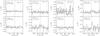 |
Fig. 3 CO tentative detections and non-detections: symbols, axis, and lines are as in Fig. 2. |
| In the text | |
|
Fig. 4 CO luminosity as a function of luminosity in different wavelength bands: Ba), FUVb), Hαc), Kd), FIRe), and 1.4 GHz f). Black and gray points and lines show subsample I and subsample II BCDs, respectively. Arrows indicate CO upper limits. Dashed and solid lines indicate linear fits to detected only and all (detected and non-detected) galaxies, respectively. |
| In the text | |
|
Fig. 5 CO luminosity as a function of stellar mass a) and Hi gas mass b). Symbols and colors are as in Fig. 4. |
| In the text | |
|
Fig. 6 Relation between CO luminosity and effective radius of the host galaxy a), and the size of the starburst emission in the optical b). Symbols and colors are as in Fig. 4. |
| In the text | |
|
Fig. 7 CO luminosity as a function of metallicity. Black dots showsubsample I while open circles showsubsample II, as well as additional very low-metallicity BCDs compiled from the literature (Fumagalli et al. 2010). Green crosses show the compilation of nearby star forming disc galaxies in Krumholz et al. (2009). Lines indicate linear best-fits to all galaxies (solid) and BCDs only (dashed). Error bars indicate typical uncertainties for our sample. |
| In the text | |
|
Fig. 8 Star-formation rate surface density as a function of H2 (left) and Hi+H2 (right) gas surface densities. Black dots showsubsample I and gray dots showsubsample II. The black dashed lines show the fits to the H2 and H2 +Hi SK law by Leroy et al. (2005) and Shi et al. (2011), respectively. Red lines indicate constant star-formation efficiencies (depletion timescales). Large arrows indicate the shift in H2 surface density by assuming a CO-to-H2 conversion factor 10 times larger than that of the Milky Way for the molecular mass. Error bars indicate typical uncertainties for our sample. |
| In the text | |
|
Fig. 9 The molecular to atomic ratio a), the molecular fraction b), and the H2 and H2 +Hi depletion timescale (c) and d), respectively) as a function of metallicity. Symbols are as in Fig. 8. Black and gray dashed lines show linear best fits to all data points and only secure detections, respectively. Solid, dotted, and dashed magenta lines in panel c show model predictions by Krumholz et al. (2011) for different values of ΣH2 + HI (80, 20 and 5 M⊙ pc-2, respectively). |
| In the text | |
|
Fig. 10 Metallicity a) and H2 depletion timescale b) as a function of specific SFR. Symbols are as in Fig. 9, but red points in a) indicate BCDs with higher gas fractions (MHI/ (MHI + M∗) > 0.5) BCDs. The dotted line in a) indicates solar metallicity, while the dashed line in b) shows the correlation found by Saintonge et al. (2011) for local star-forming disk galaxies of stellar masses M∗ ≳ 1010M⊙. |
| In the text | |
|
Fig. 11 CO-to-H2 conversion factor, αCO, as a function of the gas-phase metallicity. The right y-axis shows the ratio between the metallicity-dependent conversion factor and the constant value for the Milky Way (horizontal dashed line). A dotted vertical line indicates the solar metallicity. Black and gray dots show subsample I and subsample II BCDs, respectively, while the black solid line shows their best linear fit, indicated in the legend. Error bars indicate typical uncertainties for our sample. Red dots indicate dust-based measurements for five BCDs in our sample with Herschel data (see text). Triangles show dust-based measurements for Local Volume galaxies from Leroy et al. (2011), open circles show lower limits for the extremely metal-poor BCDs SBS 0335-052 and I Zw 18 (Hunt et al. 2014), and the magenta cross corresponds to the dIrr galaxy WLM from Elmegreen et al. (2013). Blue, red, and orange dashed lines show best fits for the same relation given by Arimoto et al. (1996), Genzel et al. (2012), and Schruba et al. (2012), respectively. The model prediction of Wolfire et al. (2010) (as presented in Sandstrom et al. 2013) is shown as a light blue band. |
| In the text | |
|
Fig. 12 Star-formation rate surface density as a function of the expected H2 (left) and Hi+H2 (right) gas surface densities after adopting the derived metallicity-dependent CO-to-H2 conversion factor αCO,Z from Eq. (2) (Fig. 11). Lines and symbols are as in Fig. 8. |
| In the text | |
|
Fig. 13 Molecular depletion timescale, as derived using αCO,Z from Eq. (2) (see text), as a function of the specific SFR. Symbols and lines are as in Fig. 10b. |
| In the text | |
|
Fig. 14 Same as Fig. 9, but using the molecular masses derived using αCO(Z) from Eq. (2) (see text). Black and gray dashed lines show linear best fits tosubsample I andsubsample II. Solid, dotted and dashed magenta (blue) lines in panel c), d) show model predictions by Krumholz et al. (2011) for different values of Σgas (80, 20 and 5 M⊙ pc-2, respectively). |
| In the text | |
Current usage metrics show cumulative count of Article Views (full-text article views including HTML views, PDF and ePub downloads, according to the available data) and Abstracts Views on Vision4Press platform.
Data correspond to usage on the plateform after 2015. The current usage metrics is available 48-96 hours after online publication and is updated daily on week days.
Initial download of the metrics may take a while.