| Issue |
A&A
Volume 586, February 2016
|
|
|---|---|---|
| Article Number | A134 | |
| Number of page(s) | 21 | |
| Section | Interstellar and circumstellar matter | |
| DOI | https://doi.org/10.1051/0004-6361/201425022 | |
| Published online | 09 February 2016 | |
Planck intermediate results
XXXI. Microwave survey of Galactic supernova remnants
1
APC, AstroParticule et Cosmologie, Université Paris Diderot,
CNRS/IN2P3, CEA/lrfu, Observatoire de Paris, Sorbonne Paris Cité, 10, rue Alice Domon et Léonie
Duquet, 75205
Paris Cedex 13,
France
2
Aalto University Metsähovi Radio Observatory and Dept of Radio
Science and Engineering, PO Box
13000, 00076
AALTO,
Finland
3
African Institute for Mathematical Sciences,
6–8 Melrose Road, Muizenberg,
7945
Cape Town, South
Africa
4
Agenzia Spaziale Italiana Science Data Center, via del Politecnico
snc, 00133
Roma,
Italy
5
Astrophysics Group, Cavendish Laboratory, University of
Cambridge, J J Thomson
Avenue, Cambridge
CB3 0HE,
UK
6
Astrophysics & Cosmology Research Unit, School of Mathematics,
Statistics & Computer Science, University of KwaZulu-Natal,
Westville Campus, Private Bag
X54001, 4000
Durban, South
Africa
7
Atacama Large Millimeter/submillimeter Array, ALMA Santiago Central
Offices, Alonso de Cordova 3107,
Vitacura, Casilla
763 0355, Santiago, Chile
8
CGEE, SCS Qd 9, Lote C, Torre C, 4° andar, Ed. Parque Cidade
Corporate, CEP
70308-200, Brasília,
DF,
Brazil
9
CITA, University of Toronto, 60 St. George St., Toronto, ON
M5S 3H8,
Canada
10
CNRS, IRAP, 9 Av.
colonel Roche, BP
44346, 31028
Toulouse Cedex 4,
France
11
California Institute of Technology, Pasadena, CA
91101
California,
USA
12
Centro de Estudios de Física del Cosmos de Aragón
(CEFCA), Plaza San Juan, 1, planta
2, 44001
Teruel,
Spain
13
Computational Cosmology Center, Lawrence Berkeley National
Laboratory, Berkeley,
CA
91101
California,
USA
14
DSM/Irfu/SPP, CEA-Saclay, 91191
Gif-sur-Yvette Cedex,
France
15
DTU Space, National Space Institute, Technical University of
Denmark, Elektrovej
327, 2800
Kgs. Lyngby,
Denmark
16
Département de Physique Théorique, Université de
Genève, 24, Quai E.
Ansermet, 1211
Genève 4,
Switzerland
17
Departamento de Física Fundamental, Facultad de Ciencias,
Universidad de Salamanca, 37008
Salamanca,
Spain
18
Departamento de Física, Universidad de Oviedo,
Avda. Calvo Sotelo s/n,
33003
Oviedo,
Spain
19
Department of Astrophysics/IMAPP, Radboud University
Nijmegen, PO Box
9010, 6500 GL
Nijmegen, The
Netherlands
20
Department of Physics & Astronomy, University of British
Columbia, 6224 Agricultural Road,
Vancouver, British
Columbia, Canada
21
Department of Physics and Astronomy, Dana and David Dornsife College
of Letter, Arts and Sciences, University of Southern California,
Los Angeles, CA
90089,
USA
22
Department of Physics and Astronomy, University College
London, London
WC1E 6BT,
UK
23
Department of Physics, Florida State University,
Keen Physics Building, 77 Chieftan
Way, Tallahassee,
Florida,
USA
24
Department of Physics, Gustaf Hällströmin katu 2a, University of
Helsinki, 00100
Helsinki,
Finland
25
Department of Physics, PrincetonUniversity,
Princeton, NJ
08544
New Jersey,
USA
26
Department of Physics, University of California,
Santa Barbara, CA
94612
California,
USA
27
Dipartimento di Fisica e Astronomia G. Galilei, Università degli
Studi di Padova, via Marzolo
8, 35131
Padova,
Italy
28
Dipartimento di Fisica e Scienze della Terra, Università di
Ferrara, via Saragat
1, 44122
Ferrara,
Italy
29
Dipartimento di Fisica, Università La Sapienza,
P. le A. Moro 2, 00185
Roma,
Italy
30
Dipartimento di Fisica, Università degli Studi di
Milano, via Celoria,
16
Milano,
Italy
31
Dipartimento di Fisica, Università degli Studi di
Trieste, via A. Valerio
2, 34128
Trieste,
Italy
32
Dipartimento di Fisica, Università di Roma Tor
Vergata, via della Ricerca Scientifica,
1
Roma,
Italy
33
Discovery Center, Niels Bohr Institute, Blegdamsvej 17, 2100
Copenhagen,
Denmark
34
Discovery Center, Niels Bohr Institute, Copenhagen
University, Blegdamsvej
17, 2100
Copenhagen,
Denmark
35
European Southern Observatory, ESO Vitacura, Alonso de Cordova 3107, Vitacura, Casilla
19001, Santiago,
Chile
36
European Space Agency, ESAC, Planck Science Office, Camino bajo del
Castillo, s/n, Urbanización
Villafranca del Castillo, Villanueva de la Cañada, 28692
Madrid,
Spain
37
European Space Agency, ESTEC, Keplerlaan 1, 2201 AZ
Noordwijk, The
Netherlands
38 Facoltà di Ingegneria, Università
degli Studi e-Campus, via Isimbardi
10, 22060
Novedrate
(CO),
Italy
39
Gran Sasso Science Institute, INFN, viale F. Crispi 7, 67100
L’Aquila,
Italy
40
Helsinki Institute of Physics, Gustaf Hällströmin katu 2, University
of Helsinki, 00100
Helsinki,
Finland
41
INAF–Osservatorio Astrofisico di Catania,
via S. Sofia 78, Catania, Italy
42
INAF–Osservatorio Astronomico di Padova,
Vicolo dell’Osservatorio 5,
Padova,
Italy
43
INAF–Osservatorio Astronomico di Roma, via di Frascati 33, Monte Porzio Catone,
Italy
44
INAF–Osservatorio Astronomico di Trieste,
via G.B. Tiepolo 11, Trieste, Italy
45
INAF/IASF Bologna, via Gobetti 101, 40126
Bologna,
Italy
46
INAF/IASF Milano, via E. Bassini 15, 20100
Milano,
Italy
47
INFN, Sezione di Bologna, via Irnerio 46, 40126
Bologna,
Italy
48
INFN, Sezione di Roma 1, Università di Roma Sapienza,
Piazzale Aldo Moro 2,
00185
Roma,
Italy
49
INFN/National Institute for Nuclear Physics,
via Valerio 2, 34127
Trieste,
Italy
50
IPAG: Institut de Planétologie et d’Astrophysique de Grenoble,
Université Grenoble Alpes, IPAG, 38000
Grenoble,
France
51
CNRS, IPAG, 38000
Grenoble,
France
52
Imperial College London, Astrophysics group, Blackett
Laboratory, Prince Consort
Road, London,
SW7 2AZ,
UK
53
Infrared Processing and Analysis Center, California Institute of
Technology, Pasadena,
CA
91125,
USA
54
Institut d’Astrophysique Spatiale, CNRS (UMR 8617) Université
Paris-Sud 11, Bâtiment
121, 91440
Orsay,
France
55
Institut d’Astrophysique de Paris, CNRS (UMR 7095),
98 bis Boulevard Arago,
75014
Paris,
France
56
Institute for Space Sciences, 077125
Bucharest-Magurale,
Romania
57
Institute of Astronomy, University of Cambridge,
Madingley Road, Cambridge
CB3 0HA,
UK
58
Institute of Theoretical Astrophysics, University of
Oslo, Blindern,
0371
Oslo,
Norway
59
Instituto de Física de Cantabria (CSIC-Universidad de
Cantabria), Avda. de los Castros
s/n, 39005
Santander,
Spain
60
Istituto Nazionale di Fisica Nucleare, Sezione di
Padova, via Marzolo
8, 35131
Padova,
Italy
61
Jet Propulsion Laboratory, California Institute of
Technology, 4800 Oak Grove
Drive, Pasadena,
California,
USA
62
Jodrell Bank Centre for Astrophysics, Alan Turing Building, School
of Physics and Astronomy, The University of Manchester, Oxford Road, Manchester, M13
9PL, UK
63
Kavli Institute for Cosmology Cambridge,
Madingley Road, Cambridge, CB3 0HA, UK
64
Kazan Federal University, 18 Kremlyovskaya St., 420008
Kazan,
Russia
65
LAL, Université Paris-Sud, CNRS/IN2P3, 91400
Orsay,
France
66
LERMA, CNRS, Observatoire de Paris, 61 Avenue de
l’Observatoire, 75014
Paris,
France
67
Laboratoire AIM, IRFU/Service d’Astrophysique – CEA/DSM – CNRS –
Université Paris Diderot, Bât. 709,
CEA-Saclay, 91191
Gif-sur-Yvette Cedex,
France
68
Laboratoire Traitement et Communication de l’Information, CNRS (UMR
5141) and Télécom ParisTech, 46 rue
Barrault, 75634
Paris Cedex 13,
France
69
Laboratoire de Physique Subatomique et Cosmologie, Université
Grenoble-Alpes, CNRS/IN2P3, 53 rue
des Martyrs, 38026
Grenoble Cedex,
France
70
Laboratoire de Physique Théorique, Université Paris-Sud 11 &
CNRS, Bâtiment 210,
91405
Orsay,
France
71
Lawrence Berkeley National Laboratory, Berkeley, CA
94720
California,
USA
72
Lebedev Physical Institute of the Russian Academy of
Sciences, Astro Space Centre, 84/32
Profsoyuznaya st., GSP-7, 117997
Moscow,
Russia
73
Max-Planck-Institut für Astrophysik, Karl-Schwarzschild-Str. 1, 85741
Garching,
Germany
74
Max-Planck-Institut für Radioastronomie,
Auf dem Hügel 69, 53121
Bonn,
Germany
75
National Radio Astronomy Observatory, 520 Edgemont Road, Charlottesville
VA
22903-2475,
USA
76
National University of Ireland, Department of Experimental
Physics, Maynooth,
Co. Kildare,
Ireland
77
Nicolaus Copernicus Astronomical Center, Bartycka 18,
00-716
Warsaw,
Poland
78
Niels Bohr Institute, Blegdamsvej 17, 2100
Copenhagen,
Denmark
79
Niels Bohr Institute, Copenhagen University,
Blegdamsvej 17, 2100
Copenhagen,
Denmark
80
Optical Science Laboratory, University College London,
Gower Street, London, UK
81
SETI Institute and SOFIA Science Center,
NASA Ames Research Center, MS
211-3, Mountain View,
CA
94035,
USA
82
SISSA, Astrophysics Sector, via Bonomea 265, 34136, Trieste, Italy
83
School of Physics and Astronomy, Cardiff University,
Queens Buildings, The Parade,
Cardiff, CF24 3AA, UK
84
Sorbonne Université-UPMC, UMR 7095, Institut d’Astrophysique de
Paris, 98 bis Boulevard
Arago, 75014
Paris,
France
85
Space Sciences Laboratory, University of California,
Berkeley, CA
94720
California,
USA
86
Special Astrophysical Observatory, Russian Academy of
Sciences, Nizhnij Arkhyz,
Zelenchukskiy region, Karachai-Cherkessian Republic, 369167, Russia
87
UPMC Univ Paris 06, UMR 7095, 98 bis Boulevard Arago, 75014
Paris,
France
88
Université de Toulouse, UPS-OMP, IRAP, 31028
Toulouse Cedex 4,
France
89
Universities Space Research Association, Stratospheric Observatory
for Infrared Astronomy, MS
232-11, Moffett
Field, CA
94035,
USA
90
University of Granada, Departamento de Física Teórica y del Cosmos,
Facultad de Ciencias, 18010
Granada,
Spain
91
University of Granada, Instituto Carlos I de Física Teórica y
Computacional, 18010
Granada,
Spain
92
Warsaw University Observatory, Aleje Ujazdowskie 4, 00-478
Warszawa,
Poland
Received: 17 September 2014
Accepted: 24 November 2015
Abstract
The all-sky Planck survey in 9 frequency bands was used to search for emission from all 274 known Galactic supernova remnants. Of these, 16 were detected in at least two Planck frequencies. The radio-through-microwave spectral energy distributions were compiled to determine the mechanism for microwave emission. In only one case, IC 443, is there high-frequency emission clearly from dust associated with the supernova remnant. In all cases, the low-frequency emission is from synchrotron radiation. As predicted for a population of relativistic particles with energy distribution that extends continuously to high energies, a single power law is evident for many sources, including the Crab and PKS 1209-51/52. A decrease in flux density relative to the extrapolation of radio emission is evident in several sources. Their spectral energy distributions can be approximated as broken power laws, Sν ∝ ν−α, with the spectral index, α, increasing by 0.5–1 above a break frequency in the range 10–60 GHz. The break could be due to synchrotron losses.
Key words: ISM: supernova remnants / cosmic rays / radio continuum: ISM
Corresponding author: W. T. Reach, This email address is being protected from spambots. You need JavaScript enabled to view it.
© ESO, 2016
1. Introduction
Supernovae leave behind remnants that take on several forms (McCray & Wang 1996). The core of the star that explodes is either flung out with the rest of the ejecta into the surrounding medium (in the case of a Type I supernova), or it survives as a neutron star or black hole (in the case of a Type II supernova). The neutron stars eject relativistic particles from jets, making them visible as pulsars and powering wind nebulae. These wind nebulae are sometimes called “plerions” and are exemplified by the Crab Nebula. Ejecta from the stellar explosion are only visible for young (~103 yr) supernova remnants (SNRs), before they are mixed with surrounding interstellar or residual circumstellar material; such objects are exemplified by the historical Tycho and Kepler supernova remnants and Cassiopeia A. Type I supernovae from white dwarf deflagration leave behind supernova remnants because their blast waves propagate into the interstellar medium. Most supernova remnants are from older explosions, and the material being observed is interstellar (and circumstellar in some cases) material shocked by the supernova blast waves. The magnetic field of the medium is enhanced in the compressed post-shock gas, and charged particles are accelerated to relativistic speeds, generating copious synchrotron emission that is the hallmark of a supernova remnant at radio frequencies.
At the highest radio frequencies and in the microwave, supernova remnants may transition from synchrotron emission to other mechanisms. The synchrotron brightness decreases as frequencies increase, and free-free emission (with its flatter spectrum) and dust emission (with its steeply rising spectrum) will gain prominence. Dipole radiation from spinning dust grains could possibly contribute (Scaife et al. 2007). Because the synchrotron radiation itself is an energy loss mechanism, the electrons decrease in energy over time, and relatively fewer higher-energy electrons should exist as the remnants age; therefore, the synchrotron emission will diminish at higher frequencies. For these reasons, a survey of supernova remnants at microwave frequencies could reveal some keys to the evolution of relativistic particles as they are produced and injected into the interstellar medium, as well as potentially unveiling new emission mechanisms that can trace the nature of the older supernova remnants.
2. Observations
2.1. Properties of the Planck survey
Planck1 (Tauber et al. 2010; Planck Collaboration I 2011) is the third generation space mission to measure the anisotropy of the cosmic microwave background (CMB). It observed the sky in nine frequency bands covering 30–857 GHz with high sensitivity and angular resolution from 31′ to 5′. The Low Frequency Instrument (LFI; Mandolesi et al. 2010; Bersanelli et al. 2010; Mennella et al. 2011) covers the 30, 44, and 70 GHz bands with amplifiers cooled to 20 K. The High Frequency Instrument (HFI; Lamarre et al. 2010; Planck HFI Core Team 2011a) covers the 100, 143, 217, 353, 545, and 857 GHz bands with bolometers cooled to 0.1 K. A combination of radiative cooling and three mechanical coolers produces the temperatures needed for the detectors and optics (Planck Collaboration II 2011). Two data processing centres (DPCs) check and calibrate the data and make maps of the sky (Planck HFI Core Team 2011b; Zacchei et al. 2011; Planck Collaboration V 2014; Planck Collaboration VIII 2014). Planck’s sensitivity, angular resolution, and frequency coverage make it a powerful instrument for Galactic and extragalactic astrophysics as well as cosmology. Early astrophysics results are given in Planck Collaboration VIII–XXVI 2011, based on data taken between 13 August 2009 and 7 June 2010. Intermediate astrophysics results are being presented in a series of papers based on data taken between 13 August 2009 and 27 November 2010.
Relevant properties of Planck are summarized for each frequency band in Table 1. The effective beam shapes vary across the sky and with data selection. Details are given in Planck Collaboration IV (2014) and Planck Collaboration VII (2014). Average beam sizes are given in Table 1. Calibration of the brightness scale was achieved by measuring the amplitude of the dipole of the cosmic microwave background (CMB) radiation, which has a known spatial and spectral form; this calibration was used for the seven lower frequency bands (30–353 GHz). At the two high frequencies (545 and 857 GHz), the CMB signal is relatively low, so calibration was performed using measurements of Uranus and Neptune. The accuracy of the calibration is given in Table 1; the Planck calibration is precise enough that it is not an issue for the results discussed in this paper.
The Planck image products are at Healpix (Górski et al. 2005) Nside = 2048 for frequencies 100–857 GHz and Nside = 1024 for frequencies 30–70 GHz, in units of CMB thermodynamic temperature up to 353 GHz. For astronomical use, the temperature units are converted to flux density per pixel by multiplication by the factor given in the last column of Table 1. At 545 and 857 GHz, the maps are provided in MJy sr-1 units, and the scaling simply reflects the pixel size.
Planck survey properties.
2.2. Flux density measurements
Flux densities were measured using circular aperture photometry. Other approaches to measuring the source fluxes were explored and could be pursued by future investigators. This includes model fitting (e.g. Gaussian or other source shape motivated by morphology seen at other wavelengths convolved with the beam) or non-circular aperture photometry (e.g. drawing a shape around the source and hand-selecting a background). We experimented with both methods and found they were highly dependent upon the choices made. The circular-aperture method used in this paper has the advantages of being symmetric about the source center (hence, eliminating all linear gradients in the background) as well as being objective about the shape of the source (hence, independent of assumptions about the microwave emitting region).
Properties of detected supernova remnants.
 |
Fig. 1 Top: Planck Images of the Crab nebula at frequencies increasing from 30 GHz at top left to 857 GHz at bottom right. Each image is 100′ on a side, with the three lowest-frequency images smoothed by 7′. Bottom: microwave spectral energy distribution of the Crab Nebula. Filled circles are Planck measurements with 3σ error bars. The open symbol at 1 GHz and the dashed line emanating from it are the flux and power law with spectral index from the Green catalogue. Open diamonds are from the compilation of flux densities by Macías-Pérez et al. (2010). |
Because of the wide range of Planck beam sizes and the comparable size
of the supernova remnants (SNRs), we took care to adjust the aperture sizes as a function
of frequency and to scale the results to a flux density scale. For each SNR, the source
size in the maps was taken to be the combination of the intrinsic source size from the
Green catalogue (Green 2009), θSNR in Table
2, and the Planck beam size,
θb in Table 1:  (1)The flux densities were measured using
standard aperture photometry, with the aperture size centred on each target with a
diameter scaled to θap = 1.5θs.
The background was determined in an annulus of inner and outer radii 1.5θap and
2θap. To correct for
loss of flux density outside of the aperture, an aperture correction as predicted for a
Gaussian flux density distribution with size θs was applied to each
measurement:
(1)The flux densities were measured using
standard aperture photometry, with the aperture size centred on each target with a
diameter scaled to θap = 1.5θs.
The background was determined in an annulus of inner and outer radii 1.5θap and
2θap. To correct for
loss of flux density outside of the aperture, an aperture correction as predicted for a
Gaussian flux density distribution with size θs was applied to each
measurement: ![Mathematical equation: \begin{equation} f_{\rm A} = \frac{1}{f(\theta_{\rm ap})-\left[f(\theta_{\rm out})-f(\theta_{\rm in})\right]} \label{eq:fap} \end{equation}](/articles/aa/full_html/2016/02/aa25022-14/aa25022-14-eq28.png) (2)where the flux density enclosed within a
given aperture is
(2)where the flux density enclosed within a
given aperture is  (3)and θin and
θout are the inner and outer radii of
annulus within which the background is measured. For the well-resolved sources (diameter
50% larger than the beam FWHM), no aperture correction was applied. Aperture corrections
are typically 1.5 for the compact sources and by definition unity for the large sources.
The use of a Gaussian source model for the intermediate cases (source comparable to beam)
is not strictly appropriate for SNRs, which are often limb-brightened (shell-like), so the
aperture corrections are only good to about 20%.
(3)and θin and
θout are the inner and outer radii of
annulus within which the background is measured. For the well-resolved sources (diameter
50% larger than the beam FWHM), no aperture correction was applied. Aperture corrections
are typically 1.5 for the compact sources and by definition unity for the large sources.
The use of a Gaussian source model for the intermediate cases (source comparable to beam)
is not strictly appropriate for SNRs, which are often limb-brightened (shell-like), so the
aperture corrections are only good to about 20%.
The uncertainties for the flux densities are a root-sum-square of the calibration uncertainty (from Table 1) and the propagated statistical uncertainties. The statistical uncertainties (technically, appropriate for white uncorrelated noise only) take into account the number of pixels in the on-source aperture and background annulus and using the robust standard deviation within the background annulus to estimate the pixel-to-pixel noise for each source. The measurements are made using the native Healpix maps, by searching for pixels within the appropriate apertures and background annuli and calculating the sums and robust medians, respectively. This procedure avoids the need of generating extra projections and maintains the native pixelization of the survey.
We verify the flux calibration scale by using the procedure described above on the well-measured Crab Nebula. The flux densities are compared to previous measurements in Fig. 1. The good agreement verifies the measurement procedure used for this survey, at least for a compact source. The Planck Early Release Compact Source Catalogue (Planck Collaboration VII 2011, hereafter ERCSC) flux density measurements for the Crab are lower than those determined in this paper, due to the source being marginally resolved by Planck at high frequencies.
Table 2 lists the basic properties of SNRs that were detected by Planck. Table 3 summarises the Planck flux-density measurements for detected SNRs. To be considered a detection, each SNR must have a statistically significant flux density measurement (flux density greater than 3.5 times the statistical uncertainty in the aperture photometry measurement) and be evident by eye for at least two Planck frequencies. Inspection of the higher-frequency images allows for identification of interstellar foregrounds for the supernova remnants, which are almost all best-detected at the lowest frequencies. A large fraction of the SNRs are located close to the Galactic plane and are smaller than the low-frequency Planck beam. Essentially none of those targets could be detected with Planck due to confusion from surrounding H ii regions. Dust and free-free emission from H ii regions makes them extremely bright at far-infrared wavelengths and moderately bright at radio frequencies. Supernova remnants in the Galactic plane would only be separable from H ii regions using a multi-frequency approach and angular resolution significantly higher than Planck. More detailed results from the flux measurements are provided in the Appendix.
As a test of the quality of the results and robustness to contamination from the CMB, we performed the flux density measurements using the total intensity maps as well as the CMB-subtracted maps. Differences greater than 1σ were seen only for the largest SNRs. Of the measurements in Table 3, only the following flux densities were affected at the 2σ or greater level: Cygnus Loop (44 and 70 GHz), HB 21 (70 GHz), and Vela (70 GHz).
3. Results and discussion of individual objects
The images and spectral energy distributions (SEDs) of detected SNRs are summarized in the
following subsections. A goal of the survey is to determine whether new emission mechanisms
or changes in the radio emission mechanisms are detected in the microwave range. Therefore,
for each target, the 1 GHz radio flux density (Green
2009) was used to extrapolate to microwave frequencies using a power law. The
extrapolation illustrates the expected Planck flux densities, if
synchrotron radiation is the sole source of emission and the high-energy particles have a
power-law energy distribution. The Green (2009) SNR
catalogue was compiled from an extensive and continuously updated literature search. The
radio spectral indices are gleaned from that same compendium. They represent a fit to the
flux densities from 0.4 to 5 GHz, where available, and are the value α in a SED
 . The spectral indices can be quite uncertain
in some cases, where observations with very different observing techniques are combined (in
particular, interferometric and single-dish). The typical spectral index for synchrotron
emission from SNRs is α ~
0.4−0.8. On theoretical grounds (Reynolds
2011), it has been shown that for a shock that compresses the gas by a factor
r, the
spectral index of the synchrotron emission from the relativistic electrons in the compressed
magnetic field has index α =
3/(2r − 2). For a strong adiabatic shock,
r = 4, so the
expected spectral index is α =
0.5, similar to the typical observed value for SNRs. Shallower spectra
are seen towards pulsar wind nebulae, where the relativistic particles are freshly injected.
. The spectral indices can be quite uncertain
in some cases, where observations with very different observing techniques are combined (in
particular, interferometric and single-dish). The typical spectral index for synchrotron
emission from SNRs is α ~
0.4−0.8. On theoretical grounds (Reynolds
2011), it has been shown that for a shock that compresses the gas by a factor
r, the
spectral index of the synchrotron emission from the relativistic electrons in the compressed
magnetic field has index α =
3/(2r − 2). For a strong adiabatic shock,
r = 4, so the
expected spectral index is α =
0.5, similar to the typical observed value for SNRs. Shallower spectra
are seen towards pulsar wind nebulae, where the relativistic particles are freshly injected.
Where there was a positive deviation relative to the radio power law, there would be an indication of a different emission mechanism. Free-free emission has a radio spectral index α ~ 0.1 that is only weakly dependent upon the electron temperature. Ionized gas near massive star-forming regions dominates the microwave emission from the Galactic plane and is a primary source of confusion for the survey presented here. Small SNRs in the Galactic plane are essentially impossible to detect with Planck due to this confusion. Larger SNRs can still be identified because their morphology can be recognized by comparison to lower-frequency radio images.
Planck integrated flux density measurements of supernova remnants.
At higher Planck frequencies, thermal emission from dust grains dominates the sky brightness. The thermal dust emission can be produced in massive star forming regions (just like the free-free emission), as well as in lower-mass star forming regions, where cold dust in molecular clouds contributes. Confusion due to interstellar dust makes identification of SNRs at the higher Planck frequencies essentially impossible without a detailed study of individual cases, and even then the results will require confirmation. For the present survey we only measure four SNRs at frequencies 353 GHz and higher; in all cases the targets are bright and compact, making them distinguishable from unrelated emission.
 |
Fig. 2 Top: images of the G21.5-0.9 environment at the nine Planck frequencies (Table 1), increasing from 30 GHz at top left to 857 GHz at bottom right. Each image is 100′ on a side, with galactic coordinate orientation. Bottom: microwave SED of G21.5-0.9. Filled circles are Planck measurements from this paper, with 3σ error bars. The open symbol at 1 GHz is from the Green catalogue. The dashed line emanating from the 1 GHz flux density is a flat spectrum, for illustration. The dotted line is a broken power law, with a break frequency at 40 GHz, a spectral index of 0.05 at lower frequencies and 0.55 at higher frequencies. Open diamonds show prior radio flux densities from Morsi & Reich (1987) and Salter et al. (1989). |
 |
Fig. 3 Top: images of the W 44 environment at the nine Planck frequencies (Table 1), increasing from 30 GHz at top left to 857 GHz at bottom right. Each image is 100′ on a side, with galactic coordinate orientation. Bottom: microwave SED of W 44. Filled circles are Planck measurements from this paper, with 3σ error bars. The open symbol at 1 GHz is from the Green catalogue, and the dashed line emanating from it is a power law with spectral index from the Green catalogue. Open diamonds are radio flux densities fromVelusamy et al. (1976) at 2.7 GHz, Sun et al. (2011) at 5 GHz and Kundu & Velusamy (1972) at 10.7 GHz. The dotted line illustrates a spectral break increasing the spectral index by 0.5 at 45 GHz to match the Planck 70 GHz flux density. Downward arrows show the flux density measurements that are contaminated by unrelated foreground emission. |
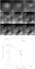 |
Fig. 4 Top: images of the CTB 80 environment at the nine Planck frequencies (Table 1), increasing from 30 GHz at top left to 857 GHz at bottom right. Each image is 100′ on a side, with galactic coordinate orientation. Bottom: microwave SED of CTB 80. Filled circles are Planck measurements from this paper, with 3σ error bars. The open symbol at 1 GHz is from the Green catalogue, and the dashed and dotted line emanating from it are power laws with spectral indices of 0.5 (Green catalogue) and 0.8 (approximate fit for 1–100 GHz), respectively, for illustration. Open diamonds are radio flux densities from Velusamy et al. (1976) at 0.75, 1.00 GHz;Mantovani et al. (1985) at 1.41, 1.72, 2.695 and 4.75 GHz; and Sofue et al. (1983) at 10.2 GHz. The downward arrow shows a flux density measurement that was contaminated by unrelated foreground emission. |
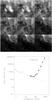 |
Fig. 5 Top: images of the Cygnus Loop environment at the nine Planck frequencies (Table 1), increasing from 30 GHz at top left to 857 GHz at bottom right. Each image is 435′ on a side, with galactic coordinate orientation. The SNR is clearly visible in the lowest-frequency images, but a nearby star-forming region (to the north) confuses the SNR at frequencies above 100 GHz. Bottom: spectral energy distribution of the Cygnus Loop including fluxes measured by us from WMAP using the same apertures as for Planck, and independent measurements from Uyanıker et al. (2004) and Reich et al. (2003). The dashed curve is a power law normalized through the radio fluxes. |
3.1. G21.5-0.9
G21.5-0.9 is a supernova remnant and pulsar wind nebula, powered by the recently-discovered PSR J1833-1034 (Gupta et al. 2005; Camilo et al. 2006), with an estimated age less than 870 yr based on the present expansion rate of the supernova shock (Bietenholz & Bartel 2008). The Planck images in the upper panels of Fig. 2 show the SNR as a compact source at intermediate frequencies. The source is lost in confusion with unrelated galactic plane structures at 30–44 GHz and at 217 GHz and higher frequencies. In addition to the aperture photometry as performed for all targets, we made a Gaussian fit at 70 GHz to the source to ensure the flux refers to the compact source and not diffuse emission. The fitted Gaussian had a lower flux (2.7 Jy) than aperture photometry (4.3 Jy), but the residual from the Gaussian fit still shows the source and is clearly an underestimate. Fitting with a more complicated functional form would yield a somewhat higher flux, so we are confident in the aperture photometry flux we report in Table 3.
The lower panel of Fig. 2 shows the Planck flux densities together with radio data. The SED is relatively flat, more typical of a pulsar wind nebula than synchrotron emission from an old SNR shock. The microwave SED has been measured at two frequencies, and the Planck flux densities are in general agreement. A single power law cannot fit the observations, as has been noted by Salter et al. (1989). Instead, we show in Fig. 2 a broken power law, which would be expected for a pulsar wind nebula, with a change in spectral index by +0.5 above a break frequency (Reynolds 2009). The data are consistent with a break frequency at 40 GHz and a relatively flat, α = 0.05 spectral index at lower frequencies.
3.2. W 44
W 44 is one of the brightest radio SNRs but is challenging for Planck because of its location in a very crowded portion of the Galactic plane. Figure 3 shows the Planck images and flux densities. The synchrotron emission is detected above the unrelated nearby regions at 30–70 GHz. Above 100 GHz, there is a prominent structure in the Planck images that is at the western (left-hand side in Fig. 3) border of the radio SNR but has a completely different morphology; we recognise this structure as being a compact H ii region in the radio images, unrelated to the W 44 SNR even if possibly due to a member of the same OB association as the progenitor. At 70 GHz, the H ii region flux is 22 Jy, comparable to the SNR; we ensured that there is no contamination of the SNR flux by slightly adjusting the aperture radius to exclude the H ii region. The Planck 70 GHz flux density is somewhat lower than the radio power law, while the 30 GHz flux density is higher. We consider the discrepancy at 30 GHz flux density as possibly due to confusion with unrelated large-scale emission from the Galactic plane. Figure 3 includes a broken power law that could explain the lower 70 GHz flux density, but the evidence from this single low flux density, especially given the severe confusion from unrelated sources in the field, does not conclusively demonstrate the existence of a spectral break for W 44.
3.3. CTB 80
CTB 80 is powered by a pulsar that has traveled so far from the centre of explosion that it is now within the shell and injecting high-energy electrons directly into the swept-up ISM. Figure 4 shows that the SNR is only clearly detected at 30 and 44 GHz, being lost in confusion with the unrelated ISM at higher frequencies. The SNR is marginally resolved at low Planck frequencies, and the flux measurements include the entire region evident in radio images (Castelletti et al. 2003). The Planck flux densities at 30 and 44 GHz are consistent with a spectral index around α ≃ 0.8, as shown in Fig. 4, continuing the trend that had previously been identified based on 10.2 GHz measurements (Sofue et al. 1983). The spectral index in the microwave is definitely steeper than that seen from 0.4 to 1.4 GHz, α = 0.45 ± 0.03 (Kothes et al. 2006), though the steepening is not as high as discussed above for pulsar wind nebulae where Δα = 0.5 can be due to significant cooling from synchrotron self-losses.
3.4. Cygnus Loop
The Cygnus Loop is one of the largest SNRs on the sky, with an angular diameter of nearly 4°. To measure the flux density, we use an on-source aperture of 120′ with a background annulus from 140′ to 170′. On these large scales, the CMB fluctuations are a significant contamination, so we subtracted the CMB using the SMICA map (Planck Collaboration XII 2014). The SNR is well detected at 30 GHz by Planck; a similar structure is evident in the 44 and 70 GHz maps, but the total flux density could not be accurately estimated at these frequencies due to uncertainty in the CMB subtraction. The NW part of the remnant, which corresponds to NGC 6992 optically, was listed in the ERCSC as an LFI source with “no plausible match in existing radio catalogues”. The actual match to the Cygnus Loop was made by AMI Consortium et al. (2012) as part of their effort to clarify the nature of such sources.
For the purpose of illustrating the complete SED, we estimated the fluxes at all Planck frequencies. Figure 5 shows the SED. The low-frequency emission is well matched by a power law with spectral index α = 0.46 ± 0.02 from 1 to 60 GHz. For comparison, a recent radio survey (Sun et al. 2006; Han et al. 2013) measured the spectral index for the synchrotron emission from the Cygnus Loop and found a synchrotron index α = 0.40 ± 0.06, in excellent agreement with the Planck results. There is no indication of a break in the power-law index all the way up to 60 GHz (where dust emission becomes important). As discussed by Han et al. (2013), previous indications of a break in the spectral index at much lower frequencies are disproved both by the 5 GHz flux density they reported and now furthermore by the 30 and 44 GHz flux densities reported here.
At high Planck frequencies, the images in Fig. 5 show bright structured emission toward the upper right corner (celestial E) and extending well outside the SNR; this unrelated emission is due to dust in molecular clouds illuminated by massive stars in the Cygnus-X region. The bright, unrelated emission makes the measurement of high-frequency fluxes of the Cygnus Loop problematic; the (heavily contaminated) aperture fluxes are well matched by a modified-blackbody fitted to the data with emissivity index β = 1.46 ± 0.16 and temperature Td = 17.6 ± 1.9 K, typical of molecular clouds. The infrared emission from the SNR shell itself was detected at 60–100 μm by Arendt et al. (1992), who derived a dust temperature of 31 K. The counterpart in the Planck images is not evident in Fig. 5. Because the dust in the SNR shell is warmer than the ISM, we can use the 545 GHz emission as a tracer of the unrelated emission and subtract it from the 857 GHz image to locate warmer dust. The subtracted image shows faint emission that is clearly associated the shell with a surface brightness (after subtracting the scaled 545 GHz image) at 857 GHz of 0.2 MJy sr-1, where the 100 μm surface brightness is 8 MJy sr-1. This surface brightness ratio can be explained by a modified blackbody for dust with a temperature Td = 31 ± 4 K and an emissivity index ≃1.5, confirming the temperature measurement by Arendt et al. (1992).
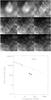 |
Fig. 6 Top: images of the HB 21 environment at the nine Planck frequencies (Table 1), increasing from 30 GHz at top left to 857 GHz at bottom right. Each image is 233′ on a side, with galactic coordinate orientation. Bottom: microwave SED of HB 21. Filled circles are Planck measurements from this paper, with 3σ error bars. The open symbol at 1 GHz is from the Green catalogue, and the dashed line emanating from it is a power law with spectral index from the Green catalogue. The dotted line is a broken power-law model discussed in the text. Open diamonds are radio flux densities from Reich et al. (2003), Willis (1973), Kothes et al. (2006), and Gao et al. (2011). The downward arrow shows a flux density measurement that was contaminated by unrelated foreground emission. |
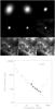 |
Fig. 7 Top: images of the Cas A environment at the nine Planck frequencies (Table 1), increasing from 30 GHz at top left to 857 GHz at bottom right. Each image is 100′ on a side, with galactic coordinate orientation. Bottom: microwave SED of Cas A. Filled circles are Planck measurements from this paper, with 3σ error bars. The open symbol at 1 GHz is from the Green catalogue, and the dashed line emanating from it is a power law with spectral index from the Green catalogue. Open circles show the flux densities from the ERCSC, the compilation by Baars et al. (1977) and Mason et al. (1999), after scaling for secular fading to the epoch of the Planck observations. |
3.5. HB 21
Figure 6 shows the microwave images and SED of the large SNR HB 21. The source nearly fills the displayed image and is only clearly seen at 30 and 44 GHz. A compact radio continuum source, 3C 418, appears just outside the northern boundary of the SNR and has a flux density of approximately 2 Jy at 30 and 44 GHz. The presence of this source at the boundary between the SNR and the background-subtraction annulus perturbs the flux density of the SNR by at most 1 Jy, less than the quoted uncertainty. The radio SED of HB 21 is relatively shallow, with α = 0.38 up to 5 GHz (Fig. 6). The Planck flux densities at 30 and 44 GHz are significantly below the extrapolation of this power law. The target is clearly visible at both frequencies, and we confirmed that the flux densities are similar in maps with and without CMB subtraction, so the low flux density does not appear to be caused by a cold spot in the CMB.
It therefore appears that the low flux densities in the microwave are due to a spectral break. For illustration, Fig. 6 shows a model where the spectral break is at 3 GHz and the spectral index changes by Δα = 0.5 above that frequency. An independent study of HB 21 found a spectral break at 5.9 ± 1.2 GHz which is reasonably consistent with our results (Pivato et al. 2013). This could occur if there have been significant energy losses since the time the high-energy particles were injected. This is probably the lowest frequency at which the break could occur and still be consistent with the radio flux densities. Even with this low value of νbreak, the Planck flux densities are over predicted. The spectral index change is likely to be greater than 0.5, which is possible for inhomogenous sources (Reynolds 2009). Given its detailed filamentary radio and optical morphology, HB 21 certainly fits in this category. The large size of the SNR indicates it is not young, so some significant cooling of the electron population is expected.
3.6. Cas A
Cas A is a very bright radio SNR, likely due to an historical supernova approximately 330 yr ago (Ashworth 1980). In the Planck images (Fig. 7), Cas A is a distinct compact source from 30–353 GHz. Cas A becomes confused with unrelated Galactic clouds at the highest Planck frequencies (545 and 857 GHz). Inspecting the much higher-resolution images made with Herschel, it is evident that at 600 GHz the cold interstellar dust would not be separable from the SNR (Barlow et al. 2010). Confusion with the bright and structured interstellar medium has made it difficult to assess the amount of material directly associated with the SNR. Figure 7 shows that from 30 to 143 GHz, the Planck SED closely follows an extrapolation of the radio power law. Cas A was used as a calibration verification for the Planck Low-Frequency Instrument, and the flux densities at 30, 44, and 70 GHz were shown to match very well the radio synchrotron power law and measurements by WMAP (Planck Collaboration V 2014).
The flux densities at 217 and 353 GHz appear higher than expected for synchrotron emission. We remeasured the excess at 353 GHz using aperture photometry with different background annuli, to check the possibility that unrelated Galactic emission is improperly subtracted and positively contaminates the flux density. At 353 GHz, the flux density could be as low as 45 Jy, which was obtained using a narrow aperture and background annulus centred on the source, or as high as 58 Jy, obtained from a wide aperture and background annulus, so we estimate a flux density and systematic uncertainty of 52 ± 7 Jy. The flux density in the ERCSC is 35.2 ± 2.0, which falls close to the radio synchrotron extrapolation. The excess flux density measured above the synchrotron prediction is 22 ± 7, using the techniques in this paper, which is significant. This excess could potentially be due to a coincidental peak in the unrelated foreground emission or to cool dust in the SNR, which is marginally resolved by Planck. Images at the lowest frequency (600 GHz) observed with the Herschel Space Observatory (Barlow et al. 2010) at much higher angular resolution than Planck show that the non-synchrotron microwave emission is a combination of both cold interstellar dust and freshly formed dust.
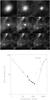 |
Fig. 8 Top: images of the Tycho SNR environment at the nine Planck frequencies (Table 1), increasing from 30 GHz at top left to 857 GHz at bottom right. Each image is 100′ on a side , with galactic coordinate orientation. Bottom: microwave SED of Tycho. Filled circles are Planck measurements from this paper, with 3σ error bars. The open symbol at 1 GHz is from the Green catalogue, and the dashed line emanating from it is a power law with spectral index from the Green catalogue. Open diamonds are a 10.7 GHz measurement from Klein et al. (1979) and Herschel flux density from Gomez et al. (2012). The dotted lines are a revised synchrotron power law with spectral index α = 0.6 at low frequency, based on the radio including 10.7 GHz and the Planck 30–143 GHz flux densities, and a modified blackbody with emissivity index β = 1 and temperature 21 K at high frequency, based on the Herschel data. Downward arrows are upper limits (99.5% confidence) to the flux density from high-frequency Planck data. The solid line is a combination of the synchrotron and dust models. |
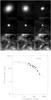 |
Fig. 9 Top: images of the 3C 58 environment at the nine Planck frequencies (Table 1), increasing from 30 GHz at top left to 857 GHz at bottom right. Each image is 100′ on a side,with galactic coordinate orientation. Bottom: microwave SED of 3C 58. Filled circles are Planck measurements from this paper, with 3σ error bars. The open symbol at 1 GHz is from the Green catalogue, and the dashed line emanating from it is a power law with spectral index from the Green catalogue. Open circles are from the Planck ERCSC. Diamonds show published flux densities: Salter et al. (1989) measured 15 ± 2 Jy at 84.2 GHz; Morsi & Reich (1987) measured 25.2 ± 1.4 Jy at 32 GHz; Green et al. (1975) measured 26.7 ± 0.5 Jy at 15 GHz; and Green (1986) measured 30 ± 3 Jy at 2.7 GHz. Flux densities from Weiland et al. (2011) are also included as open diamonds, together with a solid line showing a fit to their data. The dotted line is the broken power-law model for a pulsar wind nebula with energy injection spectrum matching the radio (low-frequency) data and a break at 25 GHz due to synchrotron cooling (see Sect. 3.8). |
 |
Fig. 10 Multi-colour Herschel/SPIRE image of 3C 58 created from images at 510 μm (587 GHz; red), 350 μm (857 GHz; green) and 250 μm (1200 GHz; blue). A white ellipse of 9′ × 5′ diameter shows the size of the radio SNR. The diffuse interstellar medium is mostly white in this image, while the emission within the ellipse is distinctly red, being brightest at 510 μm while the diffuse interstellar medium is brightest at 250 μm. The red, compact source at the centre of the ellipse is coincident with PSR J0205+6449 that is thought to be the compact remnant of the progenitor star. |
3.7. Tycho
The Tycho SNR comprises ejecta from a supernova explosion in 1572 AD. Planck detects the SNR from 30 to 545 GHz and tentatively at 857 GHz, as can be seen in the images in Fig. 8. The SED shows at least two emission mechanisms. A continuation of the synchrotron spectrum dominates the 30–143 GHz flux density, while a steeply-rising contribution, most likely due to dust, dominates above 143 GHz. The SNR is well-detected by Herschel (Gomez et al. 2012), with its excellent spatial resolution. The Herschel image shows that cold dust emission is predominantly outside the boundary of the ejecta-dominated portion of the SNR. While some is correlated with unrelated molecular clouds, much of this emission is attributed to swept-up ISM (as opposed to ejecta). From the Herschel study, the dust emission was fit with a cold component at temperature 21 K. The emissivity index of the modified blackbody that fits the Herschel and Planck SED is β = 1. (The value of the emissivity index we report, β = 1, is different from the β = 1.5 described by Gomez et al. 2012 in the text of their paper, but the cold dust model plotted in their Fig. 12 appears closer to β ≃ 1, in agreement with our Fig. 8.)
3.8. 3C 58
3C 58 is a compact source at Planck frequencies, with a 9′ × 5′ radio image size, so it becomes gradually resolved at frequencies above 100 GHz. The adopted aperture photometry and correction procedure in this survey should recover the entire flux density of this SNR at all frequencies. Figure 9 shows the SED. The flux density at 30 GHz is just a bit lower than that predicted by extrapolating the 1 GHz flux density with the radio spectral index. However, it is clear from the Planck data that the brightness declines much more rapidly than predicted by an extrapolation of the radio SED.
The Planck flux densities are in agreement with the low 84 GHz flux density that had been previously measured by Salter et al. (1989), who noted that their flux density measurement was 3σ below an extrapolation from lower frequencies. The Planck data show that the decline in flux density, relative to an extrapolation from lower frequencies, begins around or before 30 GHz and continues to at least 353 GHz.
There is a large gap in frequencies between the microwave and near-infrared detections of the pulsar wind nebula. To fill in the SED, we reprocessed the IRAS survey data using the HIRES algorithm (Aumann et al. 1990), and we find a tentative detection of the SNR at 60 μm with a flux density of 0.4 Jy. At 100 μm the SNR is expected to be brighter, but is confused with the relatively-brighter diffuse interstellar medium. In the far-infrared, we obtained the Herschel/SPIRE map, created for 3C 58 as part of a large guaranteed-time key project led by M. Groenewegen, from the Herschel Science Archive. Figure 10 shows a colour combination of the SPIRE images. The SNR is clearly evident due to its distinct colours with respect to the diffuse ISM. In addition to the diffuse emission of the SNR, there is a compact peak in the emission at the location of the pulsar J0205+6449. We measure the flux density of the SNR to be 2.1 ± 0.4 Jy using an elliptical aperture of the same size as the radio image, and we measure the compact peak from the pulsar to be 0.05 ± 0.02 Jy using a small circular aperture centred on the pulsar with a background region surrounding the pulsar and within the SNR. Table 4 summarizes the flux densities for 3C 58 from radio through infrared frequencies. For the Planck fluxes, because the source is compact, a conservative uncertainty estimate of 10% is included.
Flux densities for 3C 58.
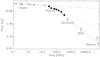 |
Fig. 11 Microwave SED of 3C 58 from the radio through infrared. Data are as in Fig. 9 with the addition of lower-frequency radio flux densities (Green 2009) and higher-frequency IRAS and Spitzer flux densities, and omission of the ERCSC flux densities. The dashed line is the power-law fit to the radio flux densities; the dotted line is the pulsar wind nebula model; and the dash-dotted line is that model with the addition of a second break with spectral index 0.92 above 200 GHz. |
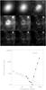 |
Fig. 12 Top: images of the IC 443 environment at the nine Planck frequencies (Table 1), increasing from 30 GHz at top left to 857 GHz at bottom right. Each image is 100′ on a side, with galactic coordinate orientation. Bottom: microwave SED of IC 443. Filled circles are Planck measurements from this paper, with 3σ error bars. The open symbol at 1 GHz is from the Green catalogue, and the dashed line emanating from it is a power law with spectral index from the Green catalogue. Open diamonds are other radio flux densities from the compilation by Castelletti et al. (2011). The dotted line is a model (dust plus broken-power-law synchrotron) discussed in the text in Sect. 3.9. The solid grey curve is an extrapolation from Onić et al. (2012). |
3C 58 is a pulsar wind nebula, like the Crab. The shallow spectral index (Sν ∝ ν− α with α = 0.07) at low frequencies is due to injection of energetic particles into the nebula from the pulsar with an energy spectrum dN/dE ∝ E− s, with s = 2α + 1 = 1.14. The electrons cool (become non-relativistic), which leads to a steepening of the spectrum, α → α + 0.5 (Reynolds 2009), above a break frequency that depends upon the magnetic field and age. As an alternative to the idea of electron cooling, breaks in the synchrotron spectral index could also simply reflect breaks in the energy distribution of the relativistic particles injected into the pulsar wind nebula. Determining the location of the microwave spectral break was deemed “crucial, as are flux measurements in the sub-mm band” (Slane et al. 2008). The present paper provides both such measurements.
The Planck flux densities match the electron-cooling model for a break frequency around 20 GHz. Figure 11 shows a wider-frequency version of the SED for 3C 58. The existence of a break in the radio spectrum was previously indicated by a measurement at 84 GHz (Salter et al. 1989) that is now confirmed by the Planck data with six independent measurements at frequencies from 30 to 217 GHz. The Wilkinson Microwave Anisotropy Probe also clearly shows the decrease in flux density at microwave frequencies (Weiland et al. 2011), and the curved spectral model from their paper is at least as good a fit to the data as the broken power law. At higher frequencies, the IRAS and Spitzer measurements are significantly over-predicted by the extrapolation of the microwave SED that matches the Planck data. Green & Scheuer (1992) had already used the IRAS upper limit to show the synchrotron spectral index must steepen before reaching the far-infrared. There may be, as indicated by Slane et al. (2008), a second spectral break. We found that a good match to the radio through infrared SED can be made with a second break frequency at 200 GHz. The nature of this second break frequency is not yet understood.
3.9. IC 443
The SNR IC 443 is well known from radio to high-energy astrophysics, due to the interaction of a blast wave with both low and high-density material. The SNR is detected at all nine Planck frequencies. The utility of the microwave flux densities is illustrated by comparing the observations of IC 443 to extrapolations based only on lower-frequency data. In one recent paper, there is a claim for an additional emission mechanism at 10 GHz and above, with thermal free-free emission contributing at a level comparable to or higher than synchrotron radiation (Onić et al. 2012). The highest-frequency data point considered in that paper was at 8 GHz. In Fig. 12 it is evident that the proposed model including free-free emission is no better fit than a power-law scaling of the 1 GHz flux density using the spectral index from the Green catalogue. The 10.7 GHz and 30 GHz flux densities are consistent with a single power law from 1–30 GHz, with the single outlier at 8 GHz being little more than 1σ away. Both the model of Onić et al. (2012) and the single power law predict the flux density at 30 GHz perfectly, but they over predict the higher-frequency emission at 40 and143 GHz by factors of more than 3 and 2, respectively. Therefore, the shape of the IC 443 SED requires a dip in emissivity in the microwave, rather than an excess due to free-free emission. The decrease in flux density could be due to a break in the synchrotron power law from the injection mechanism of the energetic particles, or due to cooling losses by the energetic particles.
At the higher Planck frequencies, another emission mechanism besides synchrotron radiation dominates the brightness. The horseshoe-shaped eastern portion of the SNR is evident with similar morphology at 100 GHz and higher frequencies. The southern part of the SNR, where shocks are impacting a molecular cloud (Rho et al. 2001), is physically distinct; this region becomes significantly brighter at frequencies of 217 GHz and above. While uncertainty in background subtraction makes an accurate flux difficult to measure, the fluxes were estimated all the way to 857 GHz for the purpose of Fig. 12. Based on the steep rise to higher frequency, and the similarity between the image at high and low frequencies, the higher-frequency emission is likely due to dust grains that survive the shock. Contamination by unrelated Galactic plane emission is significant at these frequencies. Inspecting Fig. 12, it is evident that the SNR is well detected even at the highest Planck frequencies, because it is well resolved and its spatial pattern can be recognised in the images. To determine whether the 857 GHz flux density is due to the SNR or unrelated emission, we inspect the image along the ring of the SNR, finding an average brightness of 7 Kcmb above the surrounding background, which is equivalent to an average surface brightness of 21 MJy sr-1. The solid angle of the ring is 2πθΔθ, with θ = 80′ being the radius of the SNR and Δθ ≃ 5′ being the thickness of the ring. The total flux density from this rough estimate is 3000 Jy, which is in order-of-magnitude agreement with the flux density shown in Fig. 12. This affords some quality verification of the measured flux density of the SNR dust emission.
The shape of the SED across radio and microwave frequencies can be reasonably approximated by a combination of synchrotron and dust emission. A fit to the SED shows the dust emission has a temperature of T = 16 K with emissivity index β = 1.5, where the dust emission depends on frequency as ν− βBν(T), and Bν(T) is the Planck function at temperature T. The precise values are not unique and require combination with infrared data and multiple temperature components given the complex mixture of dust in molecular, atomic, and shocked gas; dust dominates at frequencies above 140 GHz. The synchrotron emission follows a power law with spectral index of 0.36 from radio frequencies up to 40 GHz, after which the spectral index steepens to 1.5. The increase in spectral index is what makes IC 443 relatively faint in the range 70–143 GHz, compared to what might be expected from an extrapolation of the radio power law. Possible causes for spectral breaks are discussed for other SNRs in sections that follow.
3.10. Puppis A
The bright SNR Puppis A is evident in the Planck images at 30–143 GHz. The flux densities measured from the Planck images at 30–70 GHz roughly follow an extrapolation of the radio power law, suggesting the emission mechanism is synchrotron emission. The 100 GHz measurement is below the power law. While this measurement is challenging due to contamination from unrelated emission evident in images at higher frequencies, the flux density at 100 GHz does appear lower than the power law. A simple fit of a broken power law in Fig. 13 has a break frequency νbreak = 40 GHz above which the spectral index increases from 0.46 to 1.46. This fit is consistent with results from a study of WMAP observations (Hewitt et al. 2012).
 |
Fig. 13 Top: images of the Puppis A environment at the nine Planck frequencies (Table 1), increasing from 30 GHz at top left to 857 GHz at bottom right. Each image is 100′ on a side, with galactic coordinate orientation. Bottom: microwave SED of Puppis A. Filled circles are Planck measurements from this paper, with 3σ error bars. The open symbol at 1 GHz is from the Green catalogue, and the dashed line emanating from it is a power law with spectral index from the Green catalogue. Open diamonds are radio flux densities from the Milne et al. (1993) and WMAP fluxes from Hewitt et al. (2012). |
 |
Fig. 14 Top: images of the Vela environment at the nine Planck frequencies (Table 1), increasing from 30 GHz at top left to 857 GHz at bottom right. Each image is 400′ on a side, with galactic coordinate orientation, centred 1° north of Vela-X. Bottom: microwave SED of Vela. Filled circles are Planck measurements from this paper, with 3σ error bars. The open symbol at 1 GHz is from the Green catalogue, and the dashed line emanating from it is a power law with spectral index from the Green catalogue. Downward arrows show the Planck high-frequency flux density measurements that are contaminated by unrelated foreground emission. |
3.11. Vela
The very large Vela SNR is prominent in the lowest-frequency Planck images; Fig. 14 shows a well-resolved shell even at 30 GHz. The centre of the image is shifted (by 1° upward in galactic latitude) from the Green catalogue position, so as to include the entire SNR shell. The object at the right-hand edge of the lower-frequency panels of Fig. 14 is actually the previous SNR from the survey, Puppis A.
At frequencies above 70 GHz, the SNR is confused with unrelated emission from cold molecular clouds and cold cores. However, some synchrotron features remain visible at higher frequencies. The relatively bright feature near the lower centre of the image is Vela-X, the bright nest part of the radio SNR. This feature can be traced all the way to 353 GHz, with contrast steadily decreasing at higher and higher frequencies. Some dust-dominated features are visible at low frequencies. The bright feature at the centre-top of the low-frequency panels of Fig. 14 overlap with the very prominent set of knots and filaments in the high-frequency images, with a steadily decreasing brightness for the knots and filaments. At frequencies above 100 GHz, the dust features dominate here, while at 30–70 GHz the synchrotron from the SNR dominates.
The 30–70 GHz Planck flux densities follow an extrapolation of the radio power law with slightly higher spectral index, indicating the microwave emission mechanism is synchrotron, with no evidence for a spectral break.
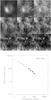 |
Fig. 15 Top: images of the PKS 1209-51/52 environment at the nine Planck frequencies (Table 1), increasing from 30 GHz at top left to 857 GHz at bottom right. Each image is 180′ on a side, with galactic coordinate orientation. Bottom: microwave SED of PKS 1209-52. Filled circles are Planck measurements from this paper, with 3σ error bars. The open symbol at 1 GHz is from the Green catalogue, and the dashed line emanating from it is a power law with spectral index from the Green catalogue. Open diamonds are radio flux densities from Milne & Haynes (1994). The downward arrow shows a Planck high-frequency flux density measurement that was contaminated by unrelated foreground emission. |
 |
Fig. 16 Top: images of the RCW 86 environment at the nine Planck frequencies (Table 1), increasing from 30 GHz at top left to 857 GHz at bottom right. Each image is 100′ on a side, with galactic coordinate orientation. Bottom: microwave SED of RCW 86. Filled circles are Planck measurements from this paper, with 3σ error bars. The open symbol at 1 GHz is from the Green catalogue, and the dashed line emanating from it is a power law with spectral index from the Green catalogue. The open diamonds is the 5 GHz flux density from Caswell et al. (1975). |
 |
Fig. 17 Top: images of the MSH 15-56 environment at the nine Planck frequencies (Table 1), increasing from 30 GHz at top left to 857 GHz at bottom right. Each image is 100′ on a side, with galactic coordinate orientation. Bottom: microwave SED of MSH 15-56. Filled circles are Planck measurements from this paper, with 3σ error bars. The open symbol at 1 GHz is from the Green catalogue, and the dashed line emanating from it is a power law with spectral index from the Green catalogue. Open diamonds are radio flux densities from the Dickel et al. (2000) and Milne et al. (1979) that constrain the slope through the Planck data. |
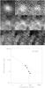 |
Fig. 18 Top: images of the SN 1006 environment at the nine Planck frequencies (Table 1), increasing from 30 GHz at top left to 857 GHz at bottom right. Each image is 100′ on a side, with galactic coordinate orientation. Bottom: microwave SED of SN 1006. Filled circles are Planck measurements from this paper, with 3σ error bars. The open symbol at 1 GHz is from the Green catalogue, and the dashed line emanating from it is a power law with spectral index from the Green catalogue. The dotted line is a broken power-law fit discussed in the text. |
3.12. PKS 1209-51/52
The barrel-shaped (Kesteven & Caswell 1987)SNR PKS1209-51/52 is detected by Planck at low frequencies. The angular structure of the SNR overlaps in spatial scales with the CMB, so PKS1209-51/52 was masked in the CMB maps. Therefore, Fig. 15 shows the total intensity for this SNR, rather than the CMB-subtracted intensity. At 30–70 GHz, the SNR is clearly evident because it is significantly brighter than the CMB and has the location and size seen in lower-frequency radio images. At 100–217 GHz, the SNR is lost in CMB fluctuations. At 353–857 GHz, the region is dominated by interstellar dust emission. The object near the centre of the SNR in the high-frequency images is a reflection nebula, identified by Brand et al. (1986, object 381) on optical places as a 3′ possible reflection nebula; it was also noted as a far-infrared source without corresponding strong H I emission (Reach et al. 1993, object 9095). There is no evidence for this object to be associated with the SNR nor the neutron star suspected to be the remnant of the progenitor (Vasisht et al. 1997, X-ray source 1E 1207.4-5209), located 12′ away. It is nonetheless remarkable that the source is right at the centre of the SNR.
Figure 15 shows the low-frequency emission seen by Planck continues the radio synchrotron spectrum closely up to 70 GHz, with no evidence for a spectral break.
3.13. RCW 86
The RCW 86 supernova remnant, possibly that of a Type I SN within a stellar wind bubble (Williams et al. 2011), is evident in the low-frequency 30–70 GHz Planck images. At higher frequencies the synchrotron emission from the SNR is confused with other emission. The feature near the left-centre of the highest 6 frequency images of RCW 86 in Fig. 16 is a dark molecular cloud, DB 315.7-2.4 (Dutra & Bica 2002). The Planck emission from this location is due to dust, with brightness steadily increasing with frequency over the Planck domain. The cloud is located near the edge of the SNR, and the CO velocity (–37 km s-1; Otrupcek et al. 2000) is approximately as expected for a cloud at the distance estimate for the SNR (2.3 kpc). Any relation between the cold molecular cloud and the SNR is only plausible; there is no direct evidence for interaction. In any event, the dust in this cloud makes it impossible to measure the synchrotron brightness at 100 GHz, and the 70 GHz flux has higher uncertainty.
For the SNR synchrotron emission, the Planck flux densities, shown in Fig. 16, are consistent within 1σ with an extrapolation of the radio synchrotron power law. The existence of X-ray synchrotron emission (Rho et al. 2002) suggests that the energy distribution of relativistic electrons continues to high energy.
3.14. MSH 15-56
The radio-bright SNR MSH 15-56 is well detected in the first five Planck frequencies, 30–143 GHz. The SNR is a “composite”, with a steep-spectrum shell and a brighter, flat-spectrum plerionic core. The Planck flux densities do not follow a single power law matching the published radio flux densities. Just connecting the 1 GHz radio flux densities to the Planck flux densities, the spectral index is in the range 0.3–0.5. The Planck flux densities themselves follow a steeper power law than can match the radio flux densities, and suggest a break in the spectral index. Figure 17 shows a broken-power-law fit, where the spectral index steepens from 0.31 to 0.9 at 30 GHz. Low-frequency radio observations show that the plerionic core of the SNR has a flatter spectral index than the shell, while higher-frequency flux densities of the core alone from 4.8 to 8.6 GHz have a spectral index of 0.85 (Dickel et al. 2000). The relatively flat spectral index at radio frequencies and up to about 30 GHz may indicate injection of fresh electrons, as in the Crab and 3C 58, which are driven by pulsar wind nebulae. However, there has been, to date, no pulsar detected in MSH 15-56, and the spectral index is not as flat as in the known, young pulsar wind nebulae. The apparent break in spectral index to a stepper slope above 30 GHz suggests possible energy loss of the highest-energy particles.
3.15. SN 1006
SN 1006 is well-detected at 30–44 GHz. At higher frequencies it becomes faint and possibly confused with unrelated emission. However, the field is not as crowded as it is for most other SNRs, and we suspect that the observed decrement in flux density below the extrapolation of the radio power law at 70 and 100 GHz may be due to a real break in the spectral index. If so, then the frequency of that break is in the range 20 <νbreak< 30 GHz. For illustration, Fig. 18 shows a broken power-law fit with νbreak = 22 GHz, above which the spectral index steepens from α = 0.5 to α = 1 as predicted for synchrotron losses. The Planck data appear to match this model well.
4. Conclusions
The flux densities of 16 known Galactic supernova remnants were measured from the Planck microwave all-sky survey with the following conclusions. We find new evidence for spectral index breaks in G21.5-0.9, HB 21, MSH 15-56, SN 1006, and we confirm the previously detected spectral break in 3C 58, including a new detection with Herschel.
Table 5 summarizes the new spectral indices required to fit the radio through microwave SED of SNRs. These values correspond to the dashed lines in the SEDs for each SNR in this paper. For each SNR in this paper for which the Planck data indicated in a spectrum noticeably different from the radio power-law extrapolation, the frequency of the spectral break (νbreak) and the spectral index at lower and higher frequencies (α1 and α2, respectively) are listed. The actual SEDs should be consulted before using the spectral index values by themselves, because they are only applicable over the region shown, and they are only mathematical approximations to what is more likely a continuous distribution of energies with evolving losses.
The breaks in spectral index are consistent with synchrotron losses of electrons injected by a central source. We extend the radio synchrotron spectrum for young SNRs Cas A and Tycho with no evidence for extra emission mechanisms. The distinction in properties between those supernova remnants that do or do not show a break in their power-law spectral index is not readily evident. The supernova remnants with spectral breaks include examples that range from bright to faint and young to mature, and they also include examples both with and without stellar remnants. A combination of cosmic-ray acceleration by the shocks and the pulsars, deceleration in denser environments, and ageing may lead to the variation in synchrotron shapes.
Sychrotron spectral indices.
Planck (http://www.esa.int/Planck) is a project of the European Space Agency (ESA) with instruments provided by two scientific consortia funded by ESA member states and led by Principal Investigators from France and Italy, telescope reflectors provided through a collaboration between ESA and a scientific consortium led and funded by Denmark, and additional contributions from NASA (USA).
Acknowledgments
The Planck Collaboration acknowledges the support of: ESA; CNES, and CNRS/INSU-IN2P3-INP (France); ASI, CNR, and INAF (Italy); NASA and DoE (USA); STFC and UKSA (UK); CSIC, MINECO, JA and RES (Spain); Tekes, AoF, and CSC (Finland); DLR and MPG (Germany); CSA (Canada); DTU Space (Denmark); SER/SSO (Switzerland); RCN (Norway); SFI (Ireland); FCT/MCTES (Portugal); ERC and PRACE (EU). A description of the Planck Collaboration and a list of its members, indicating which technical or scientific activities they have been involved in, can be found at http://www.cosmos.esa.int/web/planck/planck-collaboration.
References
- AMI Consortium, Perrott, Y. C., Green, D. A., et al. 2012, MNRAS, 421, L6 [NASA ADS] [CrossRef] [Google Scholar]
- Arendt, R. G., Dwek, E., & Leisawitz, D. 1992, ApJ, 400, 562 [NASA ADS] [CrossRef] [Google Scholar]
- Ashworth, Jr., W. B. 1980, Journal for the History of Astronomy, 11, 1 [Google Scholar]
- Aumann, H. H., Fowler, J. W., & Melnyk, M. 1990, AJ, 99, 1674 [NASA ADS] [CrossRef] [Google Scholar]
- Baars, J. W. M., Genzel, R., Pauliny-Toth, I. I. K., & Witzel, A. 1977, A&A, 61, 99 [NASA ADS] [Google Scholar]
- Barlow, M. J., Krause, O., Swinyard, B. M., et al. 2010, A&A, 518, L138 [NASA ADS] [CrossRef] [EDP Sciences] [Google Scholar]
- Bersanelli, M., Mandolesi, N., Butler, R. C., et al. 2010, A&A, 520, A4 [NASA ADS] [CrossRef] [EDP Sciences] [Google Scholar]
- Bietenholz, M. F., & Bartel, N. 2008, MNRAS, 386, 1411 [NASA ADS] [CrossRef] [Google Scholar]
- Brand, J., Blitz, L., & Wouterloot, J. G. A. 1986, A&AS, 65, 537 [NASA ADS] [Google Scholar]
- Camilo, F., Ransom, S. M., Gaensler, B. M., et al. 2006, ApJ, 637, 456 [NASA ADS] [CrossRef] [Google Scholar]
- Castelletti, G., Dubner, G., Golap, K., et al. 2003, AJ, 126, 2114 [NASA ADS] [CrossRef] [Google Scholar]
- Castelletti, G., Dubner, G., Clarke, T., & Kassim, N. E. 2011, A&A, 534, A21 [NASA ADS] [CrossRef] [EDP Sciences] [Google Scholar]
- Caswell, J. L., Clark, D. H., & Crawford, D. F. 1975, Austr. J. Phys. Astrophys. Suppl., 37, 39 [Google Scholar]
- Dickel, J. R., Milne, D. K., & Strom, R. G. 2000, ApJ, 543, 840 [NASA ADS] [CrossRef] [Google Scholar]
- Dutra, C. M., & Bica, E. 2002, A&A, 383, 631 [NASA ADS] [CrossRef] [EDP Sciences] [Google Scholar]
- Gao, X. Y., Han, J. L., Reich, W., et al. 2011, A&A, 529, A159 [NASA ADS] [CrossRef] [EDP Sciences] [Google Scholar]
- Gomez, H. L., Clark, C. J. R., Nozawa, T., et al. 2012, MNRAS, 420, 3557 [NASA ADS] [CrossRef] [Google Scholar]
- Górski, K. M., Hivon, E., Banday, A. J., et al. 2005, ApJ, 622, 759 [NASA ADS] [CrossRef] [Google Scholar]
- Green, D. A. 1986, MNRAS, 218, 533 [NASA ADS] [CrossRef] [Google Scholar]
- Green, D. A. 2009, BASI, 37, 45 (Green catalogue) [NASA ADS] [Google Scholar]
- Green, D. A., & Scheuer, P. A. G. 1992, MNRAS, 258, 833 [NASA ADS] [CrossRef] [Google Scholar]
- Green, A. J., Baker, J. R., & Landecker, T. L. 1975, A&A, 44, 187 [NASA ADS] [Google Scholar]
- Gupta, Y., Mitra, D., Green, D. A., & Acharyya, A. 2005, Curr. Sci., 89, 853 [Google Scholar]
- Han, J. L., Reich, W., Sun, X. H., et al. 2013, Inter. J. Mod. Phys. Conf. Ser., 23, 82 [CrossRef] [Google Scholar]
- Hewitt, J. W., Grondin, M.-H., Lemoine-Goumard, M., et al. 2012, ApJ, 759, 89 [NASA ADS] [CrossRef] [Google Scholar]
- Kesteven, M. J., & Caswell, J. L. 1987, A&A, 183, 118 [NASA ADS] [Google Scholar]
- Klein, U., Emerson, D. T., Haslam, C. G. T., & Salter, C. J. 1979, A&A, 76, 120 [NASA ADS] [Google Scholar]
- Kothes, R., Fedotov, K., Foster, T. J., & Uyanıker, B. 2006, A&A, 457, 1081 [NASA ADS] [CrossRef] [EDP Sciences] [Google Scholar]
- Kundu, M. R., & Velusamy, T. 1972, A&A, 20, 237 [NASA ADS] [Google Scholar]
- Lamarre, J., Puget, J., Ade, P. A. R., et al. 2010, A&A, 520, A9 [NASA ADS] [CrossRef] [EDP Sciences] [Google Scholar]
- Macías-Pérez, J. F., Mayet, F., Aumont, J., & Désert, F.-X. 2010, ApJ, 711, 417 [NASA ADS] [CrossRef] [Google Scholar]
- Mandolesi, N., Bersanelli, M., Butler, R. C., et al. 2010, A&A, 520, A3 [NASA ADS] [CrossRef] [EDP Sciences] [Google Scholar]
- Mantovani, F., Reich, W., Salter, C. J., & Tomasi, P. 1985, A&A, 145, 50 [NASA ADS] [Google Scholar]
- Mason, B. S., Leitch, E. M., Myers, S. T., Cartwright, J. K., & Readhead, A. C. S. 1999, AJ, 118, 2908 [NASA ADS] [CrossRef] [Google Scholar]
- McCray, R., & Wang, Z., eds. 1996, Supernovae and Supernova Remnants: IAU Coll. 145 (Cambridge University Press) [Google Scholar]
- Mennella, A., Butler, R. C., Curto, A., et al. 2011, A&A, 536, A3 [NASA ADS] [CrossRef] [EDP Sciences] [Google Scholar]
- Milne, D. K., & Haynes, R. F. 1994, MNRAS, 270, 106 [NASA ADS] [CrossRef] [Google Scholar]
- Milne, D. K., Goss, W. M., Haynes, R. F., et al. 1979, MNRAS, 188, 437 [NASA ADS] [CrossRef] [Google Scholar]
- Milne, D. K., Stewart, R. T., & Haynes, R. F. 1993, MNRAS, 261, 366 [NASA ADS] [CrossRef] [Google Scholar]
- Morsi, H. W., & Reich, W. 1987, A&AS, 69, 533 [NASA ADS] [Google Scholar]
- Onić, D., Urošević, D., Arbutina, B., & Leahy, D. 2012, ApJ, 756, 61 [NASA ADS] [CrossRef] [Google Scholar]
- Otrupcek, R. E., Hartley, M., & Wang, J.-S. 2000, PASA, 17, 92 [NASA ADS] [CrossRef] [Google Scholar]
- Pivato, G., Hewitt, J. W., Tibaldo, L., et al. 2013, ApJ, 779, 179 [NASA ADS] [CrossRef] [Google Scholar]
- Planck Collaboration I. 2011, A&A, 536, A1 [NASA ADS] [CrossRef] [EDP Sciences] [Google Scholar]
- Planck Collaboration II. 2011, A&A, 536, A2 [NASA ADS] [CrossRef] [EDP Sciences] [Google Scholar]
- Planck Collaboration VII. 2011, A&A, 536, A7 (ERCSC) [NASA ADS] [CrossRef] [EDP Sciences] [Google Scholar]
- Planck Collaboration IV. 2014, A&A, 571, A4 [NASA ADS] [CrossRef] [EDP Sciences] [Google Scholar]
- Planck Collaboration V. 2014, A&A, 571, A5 [NASA ADS] [CrossRef] [EDP Sciences] [Google Scholar]
- Planck Collaboration VII. 2014, A&A, 571, A7 [NASA ADS] [CrossRef] [EDP Sciences] [Google Scholar]
- Planck Collaboration VIII. 2014, A&A, 571, A8 [NASA ADS] [CrossRef] [EDP Sciences] [Google Scholar]
- Planck Collaboration XII. 2014, A&A, 571, A12 [NASA ADS] [CrossRef] [EDP Sciences] [Google Scholar]
- Planck HFI Core Team 2011a, A&A, 536, A4 [NASA ADS] [CrossRef] [EDP Sciences] [Google Scholar]
- Planck HFI Core Team 2011b, A&A, 536, A6 [NASA ADS] [CrossRef] [EDP Sciences] [Google Scholar]
- Reach, W. T., Heiles, C., & Koo, B.-C. 1993, ApJ, 412, 127 [NASA ADS] [CrossRef] [Google Scholar]
- Reich, W., Zhang, X., & Fürst, E. 2003, A&A, 408, 961 [NASA ADS] [CrossRef] [EDP Sciences] [Google Scholar]
- Reynolds, S. P. 2009, ApJ, 703, 662 [NASA ADS] [CrossRef] [Google Scholar]
- Reynolds, S. P. 2011, Ap&SS, 336, 257 [NASA ADS] [CrossRef] [Google Scholar]
- Rho, J., Jarrett, T. H., Cutri, R. M., & Reach, W. T. 2001, ApJ, 547, 885 [NASA ADS] [CrossRef] [Google Scholar]
- Rho, J., Dyer, K. K., Borkowski, K. J., & Reynolds, S. P. 2002, ApJ, 581, 1116 [NASA ADS] [CrossRef] [Google Scholar]
- Salter, C. J., Reynolds, S. P., Hogg, D. E., Payne, J. M., & Rhodes, P. J. 1989, ApJ, 338, 171 [NASA ADS] [CrossRef] [Google Scholar]
- Scaife, A., Green, D. A., Battye, R. A., et al. 2007, MNRAS, 377, L69 [NASA ADS] [Google Scholar]
- Slane, P., Helfand, D. J., Reynolds, S. P., et al. 2008, ApJ, 676, L33 [NASA ADS] [CrossRef] [Google Scholar]
- Sofue, Y., Takahara, F., Hirabayashi, H., Inoue, M., & Nakai, N. 1983, PASJ, 35, 437 [NASA ADS] [Google Scholar]
- Sun, X. H., Reich, W., Han, J. L., Reich, P., & Wielebinski, R. 2006, A&A, 447, 937 [NASA ADS] [CrossRef] [EDP Sciences] [Google Scholar]
- Sun, X. H., Reich, P., Reich, W., et al. 2011, A&A, 536, A83 [NASA ADS] [CrossRef] [EDP Sciences] [Google Scholar]
- Tauber, J. A., Mandolesi, N., Puget, J., et al. 2010, A&A, 520, A1 [NASA ADS] [CrossRef] [EDP Sciences] [Google Scholar]
- Uyanıker, B., Reich, W., Yar, A., & Fürst, E. 2004, A&A, 426, 909 [NASA ADS] [CrossRef] [EDP Sciences] [Google Scholar]
- Vasisht, G., Kulkarni, S. R., Anderson, S. B., Hamilton, T. T., & Kawai, N. 1997, ApJ, 476, L43 [NASA ADS] [CrossRef] [Google Scholar]
- Velusamy, T., Kundu, M. R., & Becker, R. H. 1976, A&A, 51, 21 [NASA ADS] [Google Scholar]
- Weiland, J. L., Odegard, N., Hill, R. S., et al. 2011, ApJS, 192, 19 [Google Scholar]
- Williams, B. J., Blair, W. P., Blondin, J. M., et al. 2011, ApJ, 741, 96 [NASA ADS] [CrossRef] [Google Scholar]
- Willis, A. G. 1973, A&A, 26, 237 [NASA ADS] [Google Scholar]
- Zacchei, A., Maino, D., Baccigalupi, C., et al. 2011, A&A, 536, A5 [NASA ADS] [CrossRef] [EDP Sciences] [Google Scholar]
Appendix A: Aperture photometry details
Aperture photometry details for Planck flux density measurements of supernova remnants.
More details on the aperture photometry are provided in Table A.1. For each flux density measurement, the following quantities are listed.
-
1
The supernova remnant (SNR) name, in the same order as inTables 2 and 3.
-
2
The observing frequency in GHz.
-
3
“Flux” is the aperture-corrected, background-subtracted flux of the source with its uncertainty. The uncertainty is a quadrature combination of the statistical uncertainty and the flux calibration uncertainty. The flux calibration uncertainty is the flux multiplied by the mission calibration uncertainty from Table 1. The statistical uncertainty is the rms of the pixel values in the background annulus, Irms, multiplied by the number of pixels in the on-source aperture and divided by the square-root of the number of pixels in the off-source annulus, then scaled by the same aperture correction as was applied to the flux.
-
4
θap is the aperture radius, within which the source flux was summed.
-
5
fA is the aperture correction factor, from Eq. (2).
-
6
Fbg is the flux of the background that was subtracted from the on-source sum of the source flux. This was calculated by taking the median brightness within the background annulus, then multiplying by the area of the on-source aperture. To aid direct comparison we also applied the same aperture correction as was applied to the source flux. Because of the long lines of sight through the Galactic disk at the locations of most of the SNRs, the backgrounds are high, and Fbg is often higher than the flux of the SNR. In itself, this is not a fundamental limitation, because a smooth background can be much brighter than the target without affecting the photometry.
-
7
Ipeak is the peak intensity in the on-source aperture, in the units of the map for which the photometry was being performed. For frequencies 30–353 GHz, the units are mK in thermodynamic CBM brightness temperature units. For 545–857 GHz, the units are MJy sr-1.
-
8
Ibg is the median intensity in the background annulus, in the same units units as Ipeak.
-
9
Irms is the standard deviation (rms) of the pixel values in the background annulus, in the same units as Ipeak. The peak, per-pixel signal-to-noise for each target can be estimated as Ipeak/Irms because the target causes the brightest pixel in the on-source aperture. This gives a quantitative measure of how readily visible the target is, at the angular scale of the Planck beam.
All Tables
Aperture photometry details for Planck flux density measurements of supernova remnants.
All Figures
|
Fig. 1 Top: Planck Images of the Crab nebula at frequencies increasing from 30 GHz at top left to 857 GHz at bottom right. Each image is 100′ on a side, with the three lowest-frequency images smoothed by 7′. Bottom: microwave spectral energy distribution of the Crab Nebula. Filled circles are Planck measurements with 3σ error bars. The open symbol at 1 GHz and the dashed line emanating from it are the flux and power law with spectral index from the Green catalogue. Open diamonds are from the compilation of flux densities by Macías-Pérez et al. (2010). |
| In the text | |
|
Fig. 2 Top: images of the G21.5-0.9 environment at the nine Planck frequencies (Table 1), increasing from 30 GHz at top left to 857 GHz at bottom right. Each image is 100′ on a side, with galactic coordinate orientation. Bottom: microwave SED of G21.5-0.9. Filled circles are Planck measurements from this paper, with 3σ error bars. The open symbol at 1 GHz is from the Green catalogue. The dashed line emanating from the 1 GHz flux density is a flat spectrum, for illustration. The dotted line is a broken power law, with a break frequency at 40 GHz, a spectral index of 0.05 at lower frequencies and 0.55 at higher frequencies. Open diamonds show prior radio flux densities from Morsi & Reich (1987) and Salter et al. (1989). |
| In the text | |
|
Fig. 3 Top: images of the W 44 environment at the nine Planck frequencies (Table 1), increasing from 30 GHz at top left to 857 GHz at bottom right. Each image is 100′ on a side, with galactic coordinate orientation. Bottom: microwave SED of W 44. Filled circles are Planck measurements from this paper, with 3σ error bars. The open symbol at 1 GHz is from the Green catalogue, and the dashed line emanating from it is a power law with spectral index from the Green catalogue. Open diamonds are radio flux densities fromVelusamy et al. (1976) at 2.7 GHz, Sun et al. (2011) at 5 GHz and Kundu & Velusamy (1972) at 10.7 GHz. The dotted line illustrates a spectral break increasing the spectral index by 0.5 at 45 GHz to match the Planck 70 GHz flux density. Downward arrows show the flux density measurements that are contaminated by unrelated foreground emission. |
| In the text | |
|
Fig. 4 Top: images of the CTB 80 environment at the nine Planck frequencies (Table 1), increasing from 30 GHz at top left to 857 GHz at bottom right. Each image is 100′ on a side, with galactic coordinate orientation. Bottom: microwave SED of CTB 80. Filled circles are Planck measurements from this paper, with 3σ error bars. The open symbol at 1 GHz is from the Green catalogue, and the dashed and dotted line emanating from it are power laws with spectral indices of 0.5 (Green catalogue) and 0.8 (approximate fit for 1–100 GHz), respectively, for illustration. Open diamonds are radio flux densities from Velusamy et al. (1976) at 0.75, 1.00 GHz;Mantovani et al. (1985) at 1.41, 1.72, 2.695 and 4.75 GHz; and Sofue et al. (1983) at 10.2 GHz. The downward arrow shows a flux density measurement that was contaminated by unrelated foreground emission. |
| In the text | |
|
Fig. 5 Top: images of the Cygnus Loop environment at the nine Planck frequencies (Table 1), increasing from 30 GHz at top left to 857 GHz at bottom right. Each image is 435′ on a side, with galactic coordinate orientation. The SNR is clearly visible in the lowest-frequency images, but a nearby star-forming region (to the north) confuses the SNR at frequencies above 100 GHz. Bottom: spectral energy distribution of the Cygnus Loop including fluxes measured by us from WMAP using the same apertures as for Planck, and independent measurements from Uyanıker et al. (2004) and Reich et al. (2003). The dashed curve is a power law normalized through the radio fluxes. |
| In the text | |
|
Fig. 6 Top: images of the HB 21 environment at the nine Planck frequencies (Table 1), increasing from 30 GHz at top left to 857 GHz at bottom right. Each image is 233′ on a side, with galactic coordinate orientation. Bottom: microwave SED of HB 21. Filled circles are Planck measurements from this paper, with 3σ error bars. The open symbol at 1 GHz is from the Green catalogue, and the dashed line emanating from it is a power law with spectral index from the Green catalogue. The dotted line is a broken power-law model discussed in the text. Open diamonds are radio flux densities from Reich et al. (2003), Willis (1973), Kothes et al. (2006), and Gao et al. (2011). The downward arrow shows a flux density measurement that was contaminated by unrelated foreground emission. |
| In the text | |
|
Fig. 7 Top: images of the Cas A environment at the nine Planck frequencies (Table 1), increasing from 30 GHz at top left to 857 GHz at bottom right. Each image is 100′ on a side, with galactic coordinate orientation. Bottom: microwave SED of Cas A. Filled circles are Planck measurements from this paper, with 3σ error bars. The open symbol at 1 GHz is from the Green catalogue, and the dashed line emanating from it is a power law with spectral index from the Green catalogue. Open circles show the flux densities from the ERCSC, the compilation by Baars et al. (1977) and Mason et al. (1999), after scaling for secular fading to the epoch of the Planck observations. |
| In the text | |
|
Fig. 8 Top: images of the Tycho SNR environment at the nine Planck frequencies (Table 1), increasing from 30 GHz at top left to 857 GHz at bottom right. Each image is 100′ on a side , with galactic coordinate orientation. Bottom: microwave SED of Tycho. Filled circles are Planck measurements from this paper, with 3σ error bars. The open symbol at 1 GHz is from the Green catalogue, and the dashed line emanating from it is a power law with spectral index from the Green catalogue. Open diamonds are a 10.7 GHz measurement from Klein et al. (1979) and Herschel flux density from Gomez et al. (2012). The dotted lines are a revised synchrotron power law with spectral index α = 0.6 at low frequency, based on the radio including 10.7 GHz and the Planck 30–143 GHz flux densities, and a modified blackbody with emissivity index β = 1 and temperature 21 K at high frequency, based on the Herschel data. Downward arrows are upper limits (99.5% confidence) to the flux density from high-frequency Planck data. The solid line is a combination of the synchrotron and dust models. |
| In the text | |
|
Fig. 9 Top: images of the 3C 58 environment at the nine Planck frequencies (Table 1), increasing from 30 GHz at top left to 857 GHz at bottom right. Each image is 100′ on a side,with galactic coordinate orientation. Bottom: microwave SED of 3C 58. Filled circles are Planck measurements from this paper, with 3σ error bars. The open symbol at 1 GHz is from the Green catalogue, and the dashed line emanating from it is a power law with spectral index from the Green catalogue. Open circles are from the Planck ERCSC. Diamonds show published flux densities: Salter et al. (1989) measured 15 ± 2 Jy at 84.2 GHz; Morsi & Reich (1987) measured 25.2 ± 1.4 Jy at 32 GHz; Green et al. (1975) measured 26.7 ± 0.5 Jy at 15 GHz; and Green (1986) measured 30 ± 3 Jy at 2.7 GHz. Flux densities from Weiland et al. (2011) are also included as open diamonds, together with a solid line showing a fit to their data. The dotted line is the broken power-law model for a pulsar wind nebula with energy injection spectrum matching the radio (low-frequency) data and a break at 25 GHz due to synchrotron cooling (see Sect. 3.8). |
| In the text | |
|
Fig. 10 Multi-colour Herschel/SPIRE image of 3C 58 created from images at 510 μm (587 GHz; red), 350 μm (857 GHz; green) and 250 μm (1200 GHz; blue). A white ellipse of 9′ × 5′ diameter shows the size of the radio SNR. The diffuse interstellar medium is mostly white in this image, while the emission within the ellipse is distinctly red, being brightest at 510 μm while the diffuse interstellar medium is brightest at 250 μm. The red, compact source at the centre of the ellipse is coincident with PSR J0205+6449 that is thought to be the compact remnant of the progenitor star. |
| In the text | |
|
Fig. 11 Microwave SED of 3C 58 from the radio through infrared. Data are as in Fig. 9 with the addition of lower-frequency radio flux densities (Green 2009) and higher-frequency IRAS and Spitzer flux densities, and omission of the ERCSC flux densities. The dashed line is the power-law fit to the radio flux densities; the dotted line is the pulsar wind nebula model; and the dash-dotted line is that model with the addition of a second break with spectral index 0.92 above 200 GHz. |
| In the text | |
|
Fig. 12 Top: images of the IC 443 environment at the nine Planck frequencies (Table 1), increasing from 30 GHz at top left to 857 GHz at bottom right. Each image is 100′ on a side, with galactic coordinate orientation. Bottom: microwave SED of IC 443. Filled circles are Planck measurements from this paper, with 3σ error bars. The open symbol at 1 GHz is from the Green catalogue, and the dashed line emanating from it is a power law with spectral index from the Green catalogue. Open diamonds are other radio flux densities from the compilation by Castelletti et al. (2011). The dotted line is a model (dust plus broken-power-law synchrotron) discussed in the text in Sect. 3.9. The solid grey curve is an extrapolation from Onić et al. (2012). |
| In the text | |
|
Fig. 13 Top: images of the Puppis A environment at the nine Planck frequencies (Table 1), increasing from 30 GHz at top left to 857 GHz at bottom right. Each image is 100′ on a side, with galactic coordinate orientation. Bottom: microwave SED of Puppis A. Filled circles are Planck measurements from this paper, with 3σ error bars. The open symbol at 1 GHz is from the Green catalogue, and the dashed line emanating from it is a power law with spectral index from the Green catalogue. Open diamonds are radio flux densities from the Milne et al. (1993) and WMAP fluxes from Hewitt et al. (2012). |
| In the text | |
|
Fig. 14 Top: images of the Vela environment at the nine Planck frequencies (Table 1), increasing from 30 GHz at top left to 857 GHz at bottom right. Each image is 400′ on a side, with galactic coordinate orientation, centred 1° north of Vela-X. Bottom: microwave SED of Vela. Filled circles are Planck measurements from this paper, with 3σ error bars. The open symbol at 1 GHz is from the Green catalogue, and the dashed line emanating from it is a power law with spectral index from the Green catalogue. Downward arrows show the Planck high-frequency flux density measurements that are contaminated by unrelated foreground emission. |
| In the text | |
|
Fig. 15 Top: images of the PKS 1209-51/52 environment at the nine Planck frequencies (Table 1), increasing from 30 GHz at top left to 857 GHz at bottom right. Each image is 180′ on a side, with galactic coordinate orientation. Bottom: microwave SED of PKS 1209-52. Filled circles are Planck measurements from this paper, with 3σ error bars. The open symbol at 1 GHz is from the Green catalogue, and the dashed line emanating from it is a power law with spectral index from the Green catalogue. Open diamonds are radio flux densities from Milne & Haynes (1994). The downward arrow shows a Planck high-frequency flux density measurement that was contaminated by unrelated foreground emission. |
| In the text | |
|
Fig. 16 Top: images of the RCW 86 environment at the nine Planck frequencies (Table 1), increasing from 30 GHz at top left to 857 GHz at bottom right. Each image is 100′ on a side, with galactic coordinate orientation. Bottom: microwave SED of RCW 86. Filled circles are Planck measurements from this paper, with 3σ error bars. The open symbol at 1 GHz is from the Green catalogue, and the dashed line emanating from it is a power law with spectral index from the Green catalogue. The open diamonds is the 5 GHz flux density from Caswell et al. (1975). |
| In the text | |
|
Fig. 17 Top: images of the MSH 15-56 environment at the nine Planck frequencies (Table 1), increasing from 30 GHz at top left to 857 GHz at bottom right. Each image is 100′ on a side, with galactic coordinate orientation. Bottom: microwave SED of MSH 15-56. Filled circles are Planck measurements from this paper, with 3σ error bars. The open symbol at 1 GHz is from the Green catalogue, and the dashed line emanating from it is a power law with spectral index from the Green catalogue. Open diamonds are radio flux densities from the Dickel et al. (2000) and Milne et al. (1979) that constrain the slope through the Planck data. |
| In the text | |
|
Fig. 18 Top: images of the SN 1006 environment at the nine Planck frequencies (Table 1), increasing from 30 GHz at top left to 857 GHz at bottom right. Each image is 100′ on a side, with galactic coordinate orientation. Bottom: microwave SED of SN 1006. Filled circles are Planck measurements from this paper, with 3σ error bars. The open symbol at 1 GHz is from the Green catalogue, and the dashed line emanating from it is a power law with spectral index from the Green catalogue. The dotted line is a broken power-law fit discussed in the text. |
| In the text | |
Current usage metrics show cumulative count of Article Views (full-text article views including HTML views, PDF and ePub downloads, according to the available data) and Abstracts Views on Vision4Press platform.
Data correspond to usage on the plateform after 2015. The current usage metrics is available 48-96 hours after online publication and is updated daily on week days.
Initial download of the metrics may take a while.