| Issue |
A&A
Volume 580, August 2015
|
|
|---|---|---|
| Article Number | A127 | |
| Number of page(s) | 15 | |
| Section | Galactic structure, stellar clusters and populations | |
| DOI | https://doi.org/10.1051/0004-6361/201424599 | |
| Published online | 18 August 2015 | |
Evolution of the Milky Way with radial motions of stars and gas
II. The evolution of abundance profiles from H to Ni
1
Institut d’Astrophysique de Paris, UMR 7095 CNRS,
Univ. P. & M. Curie, 98bis Bd
Arago,
75104
Paris,
France
e-mail: kubryk@iap.fr; prantzos@iap.fr
2
Aix-Marseille Université, CNRS, LAM (Laboratoire d’Astrophysique
de Marseille) UMR 7326, 13388
Marseille,
France
e-mail:
lia@lam.fr
Received: 14 July 2014
Accepted: 1 May 2015
Aims. We study the role of the radial motions of stars and gas on the evolution of abundance profiles in the Milky Way disk. We investigate, in a parametrized way, the impact of radial flows of gas and radial migration of stars induced mainly by the Galactic bar and its iteraction with the spiral arms.
Methods. We use a model with several new or up-dated ingredients (atomic and molecular gas phases, star formation depending on molecular gas, recent sets of metallicity-dependent stellar yields from H to Ni, observationally inferred SNIa rates), which reproduces most global and local observables of the Milky Way well.
Results. We obtain abundance profiles flattening both in the inner disk (because of radial flows) and in the outer disk (because of the adopted star formation law). The gas abundance profiles flatten with time, but the corresponding stellar profiles appear to be steeper for younger stars, because of radial migration. We find a correlation between the stellar abundance profiles and O/Fe, which is a proxy for stellar age. Our final abundance profiles are in overall agreement with observations, but slightly steeper (by 0.01−0.02 dex kpc-1) for elements above S. We find an interesting “odd-even effect” in the behaviour of the abundance profiles (steeper slopes for odd elements) for all sets of stellar yields; however, this behaviour does not appear in observations, suggesting that the effect is, perhaps, overestimated in current stellar nucleosynthesis calculations.
Key words: Galaxy: general / Galaxy: abundances / Galaxy: disk / Galaxy: evolution
© ESO, 2015
1. Introduction
The abundance profiles of chemical elements constitute one of the key properties of galactic disks. They depend on the past history of the disk and the various physical phenomena that affected it: star formation, infall and outflows, radial flows of gas, radial motions of stars, tidal interactions or mergers with other galaxies. Most semi-analytical studies of abundance profiles were performed in the framework of the so-called “independent-ring” model, where the galactic disk is simulated as an ensemble of independently evolving annuli (e.g. Guesten & Mezger 1982; Tosi 1988; Matteucci et al. 1989; Ferrini et al. 1994; Prantzos & Aubert 1995; Prantzos et al. 1996; Chiappini et al. 1997; Boissier & Prantzos 1999; Hou et al. 2000; Prantzos & Boissier 2000) and concerned the Milky Way (MW) disk, for which a large number of other constraints, both local and global ones are available. Those studies focused mainly on the interplay between the local star formation and infall rates, or on the impact of variable stellar initial mass function (IMF). They also revealed the key issue of the evolution of the abundance profile, some studies supporting a flattening of it with time (e.g. Ferrini et al. 1994; Prantzos & Aubert 1995; Hou et al. 2000) while others concluded the opposite (e.g. Tosi 1988; Chiappini et al. 1997).
The pioneering work of Tinsley & Larson (1978) and Mayor & Vigroux (1981) noticed the potential importance of radial gaseous flows for the chemical evolution of galactic disks. Lacey & Fall (1985) presented a systematic investigation of the causes of such flows, and explored the impact of such effects on the chemical evolution of the Galaxy with parametrized calculations. Further parametrized investigations with simple 1D models of disk evolution are made in, for instance Tosi (1988), Clarke (1989), Sommer-Larsen & Yoshii (1990), Goetz & Koeppen (1992), Chamcham & Tayler (1994), Edmunds & Greenhow (1995), Portinari & Chiosi (2000) and more recently in Spitoni & Matteucci (2011), Bilitewski & Schönrich (2012), Mott et al. (2013), Cavichia et al. (2014). They have various motivations (mostly to study the abundance profiles, but also gas and star profiles) and they are generally applied to the study of the MW disk. As expected, results are not conclusive, because they depend not only on the parametrization of the unknown inflow velocity patterns, but also on the other unknown (and parameterized) ingredients of the models, especially the adopted star formation rate (SFR) and infall profiles as functions of time.
Amongst the alleged causes of radial inflows, the impact of a galactic bar is well established, both from simulations and from observations. Numerical simulations (Athanassoula 1992; Friedli & Benz 1993; Shlosman & Noguchi 1993) have shown that the presence of a non-axisymmetric potential from a bar can drive important amounts of gas inwards of corotation (CR) fuelling star formation in the galactic nucleus, while at the same time gas is pushed outwards outside corotation. In a disk galaxy, this radial flow mixes gas of metal-poor regions into metal-rich ones (and vice versa) and may flatten the abundance profile − (e.g. Friedli et al. 1994; Zaritsky et al. 1994; Martin & Roy 1994; Dutil & Roy 1999) − although Sánchez et al. (2012) find little difference in that respect between barred and non-barred disks. The study of Kubryk et al. (2013) suggests that bars may be changing the chemical abundance profile inside the corotation radius but they only have a small impact outside it, while Martel et al. (2013) find a rather complex situation of continuous exchange of gas and metals between the bar and the central region of the disk.
The investigation of radial motions of stars − which is due to inhomogeneities of the galactic gravitational potential − on the chemical evolution of disks, has a more recent history. The role of the bar has been studied to some extent with N-body+SPH codes by Friedli & Benz (1993) and Friedli et al. (1994). The properties of the MW bar (which was revealed by observations in the 90ies, e.g. Blitz & Spergel 1991), i.e. its size and age, are not well known yet, and its role in the overall evolution of the Galaxy is poorly understood. On the other hand, Sellwood & Binney (2002) showed that recurring transient spirals may induce important radial displacements of the corotating stars in a galactic disk, scattering them to different galactocentric radii (inwards or outwards); overall angular momentum distribution is preserved by the process, which does not contribute to the radial heating of the stellar disk. In contrast, the process can increase the dispersion in the local metallicity vs. age relation, well above the amount due to the epicyclic motion. Minchev & Famaey (2010) suggested that resonance overlap of the bar and spiral structure (Sygnet et al. 1988) produces a more efficient redistribution of angular momentum in the disk. This bar-spiral coupling has been studied in detail with N-body simulations by Brunetti et al. (2011) who found that radial migration can be described as a diffusion process with time- and position-dependent diffusion coefficients. Kubryk et al. (2013) confirmed that with a N-body+SPH simulation of a disk galaxy and showed that radial migration may have a strong impact on the chemical evolution of the disk, by moving around some long-lived sources of nucleosynthesis (SNIa and AGB stars).
The implications of radial migration for the chemical evolution of MW-type disks were studied with N-body codes by Roškar et al. (2008), who found that the stellar abundance profiles flatten with stellar age; thus their evolution does not reflect faithfully the one of the gaseous abundance profiles: gas has steep profiles early on in inside-out models of disk galay evolution, but radial migration makes them progressively flatter. Schönrich & Binney (2009) used a semi-analytical chemical evolution code and introduced a parametrised prescription of radial migration. They suggested that radial mixing could also explain the formation of the Galaxy’s thick disk, with a kinematically “hot” stellar population from the inner disk being brought in the solar annulus. Subsequent investigations with N-body models lead to controversial results: Loebman et al. (2011) find that radial migration may explain the properties of the local thick disk, while Minchev et al. (2012) find such secular processes insufficient and propose external agents (e.g. early mergers) for that.
Following the pioneering work of Schönrich & Binney (2009), the properties of the MW disk were studied in detail with semi-analytical models accounting for radial migration by Minchev et al. (2013) and Kubryk et al. (2015). The three models differ in several ways: Schönrich & Binney (2009) use a toy-model of star transfer between adjacent radial zones (with coefficients tuned to reproduce properties of the local disk), whereas the other two are inspired by the results of N-body simulations (but they adopt different implementation techniques of those results). Radial gaseous flows are included in Schönrich & Binney (2009) and Kubryk et al. (2015), but not in Minchev et al. (2013); however, in Schönrich & Binney (2009) the radial flows mainly concern the outer disk, where in Kubryk et al. (2015) they concern the inner disk, since that work simulates the action of a bar. The dimension vertical to the galactic plane is considered in Schönrich & Binney (2009) and Minchev et al. (2013), but not in Kubryk et al. (2015). Finally, the star formation and radial infall laws are different in the three works. All models explicitly consider Fe production by SNIa (albeit with different prescriptions for the SNIa rate) and the finite lifetimes of stars.
Despite those differences, all three models find good agreement with the main observables of the MW, both locally (dispersion in age-metallicity relation, metallicity distribution, the characteristic “two-branch” behaviour between thick and thin disk in the O/Fe vs. Fe/H plane) and globally (stellar and abundance profiles). This agreement suggests that, despite their sophistication, such models still involve too many parameters and suffer from degeneracy problems. We note here the difference in the final abundance gradient of Fe/H between Schönrich & Binney (2009) and Minchev et al. (2014), who find slopes of the corresponding exponential profiles of −0.1 dex kpc-1 and −0.06 dex kpc-1, respectively. Recent observations of statistically significant samples of Cepheids are consistent with the latter value, as we discuss in Sect. 3.
In this work, we study the evolution of abundance profiles of all elements from H to Ni in the MW, using the model presented in Kubryk et al. (2015, hereafter KPA15). The plan of the paper is as follows: the main ingredients of the model are briefly presented in Sect. 2, where we also discuss some of the results concerning the impact of radial migration on the disk properties. We illustrate that impact by comparing a model with radial migration to one without it. In Sect. 3 we discuss in some detail the profiles of the most important metals, namely O (Sect. 3.1) and Fe (Sect. 3.2) and we compare them to a large number of recent observations from various metallicity tracers. The impact of radial migration on the evolution of the abundance profiles is discussed in Sect. 3.3, where we compare our results to those of a similar study (Minchev et al. 2014) and to a compilation of extragalactic observations by Jones et al. (2013). In Sect. 3.4 we address the issue of the O/Fe ratio; in view of the small dispersion displayed by that ratio as a function of time, it can be used as a robust proxy for stellar age in studies of the evolution of the abundance profiles in the disk. In Sect. 3.5 we present our results for all elements from H to Ni and we compare them to several sets of observational data. We find good overall agreement with observations, but a systematically steeper (in absolute value) slope of the abundance profiles for the Fe-peak elements compared to observations. We also reveal − and we draw attention to − interesting differences between the results obtained with different sets of stellar yields, as well as a manifestation of the “odd-even” effect of nucleosynthesis, which does not appear, however, in the observational data. A summary of the results is presented in Sect. 4.
2. The model
The model presented in Kubryk et al. (2015, hereafter KPA15) for the evolution of the MW disk, involves radial motions of both gas and stars. The MW disk is built gradually by infall of primordial gas1 in the potential well of a “typical” dark matter halo of final mass 1012M⊙, the evolution of which is extracted from numerical simulations (from Li et al. 2007). The infall rate is a parametrized function, its timescale increasing monotonically with galactocentric radius and ranging from 1 Gyr at 1 kpc to 7 Gyr at 7 kpc and slightly increasing further outwards (see Fig. 1). Star formation depends on the local surface density of molecular gas, which is calculated by the semi-empirical prescriptions of Blitz & Rosolowsky (2006): it depends on a combination of the stellar surface density profile (steeply decreasing with radius) and the gas surface density profile (essentially flat today). This allows us to use the final profiles of atomic and molecular gas as supplementary constraints to the model (see Fig. 6 in KPA15). The adopted prescription produces a steep profile of H2 (as observed in the Galaxy) and a steep SFR profile in the inner disk during most of the Galactic evolution. This affects directly the corresponding abundance profiles, as we discuss below. For the radial flows of gas, we consider only the case of a MW-like bar operating for the past 6 Gyr and driving gas inwards and outwards from corotation. The radial velocity profile of the gas flow induced by the bar is similar to the one adopted in Portinari & Chiosi (2000, their Case B for the bar), but not exactly the same. Portinari & Chiosi (2000) consider additional radial flows inwards, acting all over the disk, while we limit ourselves to the case of the bar alone. The adopted radial velocity profile is given in Fig. 1.
We considered the epicyclic motion of stars (blurring) separately from the true variation in their guiding radius (churning), as in Schönrich & Binney (2009). For the former, we developed an analytic formalism based on the epicyclic approximation; for the latter, we adopted a parametrised description, using time- and radius-dependent diffusion coefficients, extracted from the N-body+SPH simulation of Kubryk et al. (2013), which concerns a disk galaxy with a strong bar. As discussed in KPA15, we adapted those transfer coefficients taking the smaller size of the MW bar into account. For the chemical evolution, we adopted recent sets of metallicity-dependent yields from Nomoto et al. (2013), providing a homogeneous and fine grid of data, which is well adapted to the case of the MW disk. For comparison purposes, we also used older yields from Woosley & Weaver (1995) and Chieffi & Limongi (2004). We adopted the stellar IMF of Kroupa (2002) with a slope of X = 1.7 (the Scalo slope) for the high masses. For the rate of SNIa, we adopted the empirical law of RSNIa ∝ t-1.1, after the observed delayed time distribution of those objects in external galaxies (see e.g. Maoz et al. 2012, and references therein). In contrast to usual practice in studies of galactic chemical evolution, we adopted the formalism of single particle population (SPP), which is the only one applicable to the case of radial migration, since it allows one to consider the radial displacements of nucleosynthesis sources and in particular of SNIa (see Kubryk et al. 2013, for a discussion of that effect). Finally, we adopted a large and diverse set of recent observational data to constrain our model.
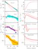 |
Fig. 1 Left (from top to bottom): model profiles of stars, gas, SFR and molecular gas fraction fMol at 4, 8 (thin curves) and 12 Gyr (thick curve). The curve at 12 Gyr is compared to observational data for the present-day profiles of the correspoding quantities (shaded aereas for the stars, gas and fMol and points with error bars for the SFR); data sources are provided in KPA15. Right (from top to bottom): infall timescales, infall rates, velocity profiles of radial inflow (positive values towards the Galactic centre), ratio of SNIa/CCSN; in all panels but the top one, the three curves correspond to 4, 8 and 12 Gyr (thickest curve). |
Our model reproduces the current values of most of the main global observables of the MW bulge (assumed to correspond to radii r< 2 kpc) and disk (r> 2 kpc): present-day masses of stars, atomic and molecular gas, SFRs and core collapse supernova (CCSN) and SNIa rates (see Fig. 2 in KPA15). The corresponding radial profiles of all those quantities (azimuthally averaged) are also reproduced in a satisfactory way (Fig. 6 in KPA15). The azimuthally averaged radial velocity of gas inflow in the bar region is constrained to be less than a few tenths of km/s in the framework of that model. The local properties of the MW disk, i.e. metallicity distribution and age-metallicity relation, are also reproduced well. In particular, following Sellwood & Binney (2002), we showed how radial migration can be constrained by the observed dispersion in the age-metallicity relation. We emphasise, however, that the observational samples that we used − from Bensby et al. (2014) for the age-metallicity relation and from Adibekyan et al. (2011) and Bensby et al. (2014) for the metallicity distribution − have various selection biases (kinematic, limited by magnitude or volume), which have not been applied to our results: the model predictions for the solar neighbourhood concern the “solar cylinder”, of diameter 0.5 kpc (the size of our radial bin), centred on the Sun.
Assuming that the thick disk is the oldest (>9 Gyr) part of the disk, we found that the adopted radial migration scheme can reproduce quantitatively the main local properties of the thin and thick disks: metallicity-distributions, the characteristic “two-branch” behaviour of the local O/Fe vs. Fe/H relation, local surface densities of stars (10 M⊙/pc2 and 28 M⊙/pc2 for the thick and thin disk, respectively). The thick disk extends up to ~11 kpc and has a scale length of 1.8 kpc; this is consistent with recent evaluations (e.g. Bovy & Rix 2013, and references therein) and it is considerably shorter than the one of the thin disk, consistent with the inside-out formation scheme.
Some of the main results of the model relevant for this work appear in Fig. 1. The inside-out formation of the disk is shown by the evolution of both the infall rate profile and the stellar profile. The gaseous profile, mostly flat today, with a local surface density of ~12 M⊙/pc2, is reproduced. The profile of the molecular fraction  is also reproduced well, after the prescriptions of Blitz & Rosolowsky (2006). As already mentioned, this profile plays an important role in our model, because it determines the molecular profile and, hence the profile of the SFR Ψ(r) = fMol(r)ΣGas(r).
The profile of the SNIa/CCSN ratio (bottom right panel) becomes steeper as one moves from the outer to the inner Galaxy, because the SNIa rate − which is a mixture of old and young population objects − follows a combination of the stellar and gas profiles. The steep stellar profile increases the SNIa/CCSN ratio in the inner disk substantially. The outer disk, populated mostly by gas and young stars, essentially has SNIa belonging to the young stellar population, as the CCSN: as a result, the SNIa/CCSN ratio in the outer disk is practically constant. Similar results for the SNIa/CCSN ratio are obtained in the independent-ring model for the MW disk by Boissier & Prantzos (2009), both with the numerical prescription of Greggio (2005) and with an analytical prescription for the SNIa rate (their Fig. 11). In the present study, a fraction of SNIa − those belonging to the old stellar population − is affected by radial migration, mostly in the region 3−12 kpc (see next paragraph). All these features directly affect the resulting O and Fe profiles, as well as those of all other elements (see discussion in next section).
Some aspects of the stellar radial migration of the model appear in Fig. 2. It can be seen that the action of the bar brings a large fraction of the stars in the inner disk into the outer regions. Some stars born in r = 3 kpc are found in the solar neighbourhood at the end of the simulation. As we show in KPA15, these are the most metallic stars presently found in the solar annulus, with metallicities [ Fe / H ] ~ 0.4 and they are 3−5 Gyr old. In contrast, a negligible fraction of the stars born in r> 12 kpc reaches the solar circle2.
As can be seen in the third panel of Fig. 2, stars found in the radial range 3−14 kpc have been formed, on average, inwards from their present position. The effect is most pronounced for stars in the region 6−9 kpc, where the average outwards displacement reaches Δr ~ 1.5 kpc, and it is reduced to negligible values inside 4 kpc and outside 14 kpc. Also, the dispersion around those average values is large in the 6−9 kpc range and decreases outside it. Clearly, however, radial migration affects regions at all galactocentric distances to some extent. We stress that the extent of radial migration depends strongly on the adopted (time- and radius-dependent) diffusion coefficients and on the morphology of the disk galaxy: a larger amount of radial migration is expected in the case of barred disks, through the coupling of the bar to the spiral arms (Minchev & Famaey 2010).
Finally, the average age of stars in the region 4−9 kpc is modified by radial migration (bottom panel in Fig. 2): the age of stars formed in situ varies little with radius outside r = 6 kpc, because the adopted profile of the infall timescale (Fig. 1) varies little in that region. However, radial migration brings older (on average) stars from the inner disk in intermediate radii: as a result, a clear age gradient is developed throughout the disk (Fig. 2 bottom).
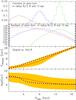 |
Fig. 2 Top: fractions of stars born in radii rOrigin = 3, 8 and 13 kpc and found in radius rFinal at t = 12 Gyr. 2nd row: numbers of stars born in annuli of radius rOrigin = 3, 8 and 13 kpc and width Δr = 0.5 kpc and found in radius rFinal at t = 12 Gyr. 3d row: Original vs. final guiding radii of stars (solid curve); the shaded area includes ±1σ values (i.e. from 16% to 84% of the stars) and the dotted diagonal line indicates the stellar guiding radii in the absence of radial migration. Bottom: average age of stars vs. Galactocentric radius (solid curve); the shaded aerea includes ±1σ values and the dotted curve indicates the average age of stars formed in situ. |
As emphasized in KPA15, the impact of radial migration on the properties of the disk is not intuitively straightforward, because migrating stars may return their gas (metal-rich, if originating in the inner disk or metal-poor if originating in the outer disk) in places far away from their home radius. This gas may affect the local metallicity and also fuel star formation (depending on the local star formation efficiency). The situation becomes even more complex in the case of a bar, because the bar drives gas inwards. This gas is more metal poor, in general, than the local gas and fuels star formation in the inner disk, making the metallicity in the inner disk to decrease. The overall result also depends on the ratio of the local infall rate to the SFR and on the previous history of the disk (which determines the metallicity at any given time). Oxygen is affected differently than Fe, because the main source of the latter, namely SNIa, is affected by radial migration, while the source of O (massive stars) is not.
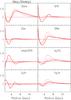 |
Fig. 3 Top: comparison of various properties of our model, expressed as the ratio of a given quantity in the case of radial migration to the same quantity when stars do not migrate. From top to bottom, left: star surface density, gas surface density, gas fraction, O/H profile; right: SFR surface density, SNIa rate, ratio of SNIa/CCSN, Fe/H profile. In all panels, thick curves represent results at 12 Gyr and thin curves at 8 and 4 Gyr, respectively (as in Fig. 1). |
We attempt an illustration of this complex behaviour in Fig. 3, where we plot the ratio of several quantities of the model (with radial migration and radial inflow) to those same quantities obtained by an identical model (same boundary conditions, same SFR and infall rates) without radial migration or radial inflow. One can easily see that the quantities affected mostly by radial migration are the long-lived stars and SNIa and their radial profiles are affected over most of the disk. The radial profiles of SNIa are affected to a smaller extent than those of stars, because a substantial fraction of SNIa results from a young population, unaffected by radial migration (~40% of them explode within 1 Gyr after the formation of their progenitor system, see Fig. C1 of Kubryk et al. (2015); in contrast, most stars are low-mass and long-lived (~90% by number for a normal IMF) and their population is affected by radial migration.
Gas is mainly affected not by radial migration, but by the radial inflow induced by the bar. Its surface density is depleted in the 2−4 kpc region and slightly increased outside it. The latter increase is to a small extent, also due to the gas returned to the interstellar medium (ISM) by the migrating, dying stars. The evolution of the gas profile is reflected in the one of the SFR profile, which is also affected by the radially dependent fraction fH2 of molecular gas, because there is less SFR in the 2−4 kpc region than without radial migration and gas inflow. That region is also the one that corresponds to the peak of the infall rate during the late evolution of the disk (see Fig. 1), and it shows a higher infall/SFR ratio than the model with no radial migration. For those reasons (lower SFR and higher dilution of the metallicity through the primordial infall), this region is found to have a lower O/H ratio than in the model with no radial migration. The decrease in the Fe/H ratio is smaller, because some Fe is contributed in those zones by SNIa migrating inwards. But the largest impact on the chemical evolution concerns the SNIa migrating outwards: they increase the Fe content of the region between 5 and 8 kpc by ~30% after 4 Gyr and by ~10% in the end of the simulation. As a result, the final Fe/H radial profile is somewhat steeper than in the model without radial migration.
Overall, the effects of radial migration on the profiles of stars, SNIa, SNIa/CCSN ratio and Fe/H appear to become less important at late times. This result appears counter-intuitive, at first sight, because more radial migration occurs on longer timescales (everything else kept equal). Our counter-intuitive result is due to the inside-out formation of the disk. At early times, there are few stars (and SNIa) in the outer Galaxy: any radial transfer from the inner regions (where a large stellar population has been formed) to the outer ones, increases the surface density of the latter by a large amount. At late times, the stellar population is in place throughout the disk: the impact of radial migration from the inner to the outer disk (where a lot of stars are formed in situ) is proportionally weaker then.
Kubryk et al. (2013) performed a similar exploration of the effects of radial migration for the case of an N-body+SPH simulation concerning a barred disk galaxy, evolving without gaseous infall (as a closed box). They found, in that case, that the strong bar induced a much larger amount of radial migration throughout the disk, affecting particularly its outmost regions. As discussed in KPA15, we adapted the description of the radial migration of that model to the one of the MW, by taking the size of the bar in the two cases into account. The smaller bar of the MW implies a smaller extent of radial migration than in the barred disk of Kubryk et al. (2013).
3. Abundance evolution
Our model includes the detailed evolution of 83 isotopes, from H to Zn. The abundances of the corresponding 32 elements are obtained at each time step by summing over the isotopic ones.
In KPA15 we have found that the adopted parameters of the model (SFR efficiency, infall timescale, SNIa rate, IMF, etc.) allow us to reproduce the solar abundance of O and Fe for the average 4.5 Gyr old star in the solar neighbourhood3 The average birth radius of those stars is found to be at a Galactocentric distance of ~6.5 kpc, i.e. ~1.5 kpc inwards from the present day position of the Sun. This implies that the Sun is an average star of 4.5 Gyr in the solar neighbourhood as far as its chemistry is concerned, but such stars are not born in situ, they have migrated here from the inner disk.
Regarding the other elements and isotopes, we find that the agreement with the solar abundances is quite good for most of them (to better than a factor of 2, see Fig. 17 in KPA15). In several cases, however, and in particular in the region of Sc to Mn, a clear underabundance is obtained with the adopted yields of Nomoto et al. (2013). The reason for that disagreement is obviously a deficiency in the yields. A similar deficiency is obtained when using those yields to study the evolution of the halo (see Fig. 10 in Nomoto et al. 2013). To cure for that, we normalised the model results as to have the average abundances of the 4.5 Gyr old stars currently present in the solar neighbourhood equal to their solar values, i.e. we corrected the stellar yields (integrated over the IMF) to various degrees (by 2% for O, up to a factor of 4 for V). In that way, we were able to compare the corresponding evolution of all the abundance ratios X/Fe vs. Fe/H to observational data from two recent surveys (Adibekyan et al. 2011; Bensby et al. 2014) concerning the local thin and thick disks separately. We showed how such detailed comparisons in the future will provide valuable constraints to both stellar nucleosynthesis and chemical evolution models.
Here we extend the investigation of the abundance evolution to the whole disk for all the elements of our model and leave the isotopic evolution for a future paper. We use abundance data from various sources and different classes of objects: Cepheids, B-stars, HII regions, planetary nebulae (PN), and open clusters. The first three concern young objects: Cepheids have masses >3 M⊙ and, depending on their metallicity, they are younger than 300−400 Myr, while B-stars and HII regions are less than a few 107 Myr old; on the other hand, PN and open clusters correspond to objects with ages up to several Gyr. The sources of the adopted data are presented in Table 1.
References for adopted data on Cepheids, B-stars, HII-regions, planetary nebulae (PN), and open clusters (OC).
3.1. Oxygen profiles
Oxygen is a major product of the nucleosynthesis of massive stars (M> 10M⊙). Because they are short-lived (lifetime <20 Myr), such stars have no time to migrate away from their birth sites (less than a 100 pc) as suggested by the fact that all CCSN localised up to now in external galaxies are within spiral arms and/or regions of active star formation. As a result, the radial O profile is not affected by radial migration. It is strongly affected, however, by gas radial inflows, as found in numerous studies, with semi-analytical and N-body+SPH models, e.g. Mayor & Vigroux (1981), Lacey & Fall (1985), Tosi (1988), Friedli et al. (1994), Portinari & Chiosi (2000), Spitoni & Matteucci (2011), Bilitewski & Schönrich (2012), Cavichia et al. (2014), etc. The results presented here depend directly on the adopted treatment of radial inflow, which corresponds to the action of the galactic bar, as described in Sect. 2. Among the aforementioned studies, only Portinari & Chiosi (2000) and Cavichia et al. (2014) explicitly considered radial flows induced by the Galactic bar.
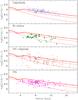 |
Fig. 4 Oxygen abundance profiles of Cepheids, B-stars, HII regions, and planetary nebulae (PN); data sources are in Table 1. The adopted solar value of log (O / H) + 12 = 8.73 is from Asplund et al. (2009). Model curves (from bottom to top, in all panels) represent the gaseous abundance profile at times 4, 8 and 12 Gyr (thick curve), respectively. |
In Fig. 4 we display the evolution of the gaseous profile of oxygen in our model. The O profile results from the joint action of three different factors:
-
the inside-out formation of the disk, affected by both the adopted infall profile (shorter timescale in the inner disk, Fig. 1, top right) and the greater efficiency of star formation in the inner disk (because of the larger molecular fraction there, Fig. 1, bottom left).
-
the radial inflow, which affects the gaseous profile and all the abundance profiles in the inner galaxy (r< 6 kpc).
In the 2−4 kpc region, the combination of the action of the bar (which pushes gas partly towards the centre and partly towards the outer disk) and the metal-poor infall leads to a local depression of O/H with respect to adjacent regions. This is because the O-rich gas pushed inwards and outwards from that region is replenished by the metal-poor infall, the rate of which happens to be at maximum in that region (Fig. 1). In adjacent regions the effect is weaker, because the late infall rate is less intense there.
The disk beyond radius r ~ 6 kpc is not affected by radial inflows. The resulting O/H profile is smoothly decreasing outwards, but it cannot be described by a single exponential over the whole radial range: its slope is steeper at small radii and flatter at larger ones. If it is fitted with a single exponential, then the slope depends on the radial range considered. In this work, we shall consider the range 5−14 kpc, where most of the observational data are available.
There are several shortcomings and uncertainties in the analysis of the observed O abundances of different types of objects across the Galactic disk, which are presented in the recent monograph of Stasińska et al. (2012). The various surveys lead to widely different results for the O/H abundance gradient dlog (O / H) / dr (in dex kpc-1), ranging from low values (−0.023 ± 0.06 in the PN sample of Stanghellini & Haywood 2010 in the 2−17 kpc range) to high ones (−0.056 ± 0.013 in the Cepheid sample of Luck & Lambert 2011 in the 5−16 kpc range).
In Fig. 4 we compare our results to the data of some recent, representative surveys, of those tracers. We do not plot all the data in the same figure, since this would create confusion and artificially increase the scatter, because of systematic uncertainties between different analysis techniques (see Stasińska et al. 2012). It can be seen that our results are in overall agreement with the various observations. There are practically no data that correspond to the inner disk (r< 4 kpc), where our model predicts lower values than in adjacent reasons, as discussed above. We notice, however, that in their study of PN in the direction of the Galactic bulge, Chiappini et al. (2009) identified a subsample of 44 objects that actually belong to the inner disk population (a few kpc from the Galactic centre) and have an average value of log (O / H) + 12 = 8.52 ± 0.23, i.e. less than expected from the extrapolation of the Henry et al. (2010) data for PN in that region. It is not yet clear whether that difference is due to systematic uncertainties between the two studies −Chiappini (2009) collected line intensities from the literature, unlike Henry et al. (2010)− or to a genuine decline in the oxygen profile in the inner disk, in qualitative agreement with our results.
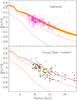 |
Fig. 5 Iron abundance profiles of Cepheids (top) and open clusters (bottom). Data sources are provided in Table 1. Symbols in the upper panel correspond to Ref. 3 and in the lower panel to Refs. 9 (blue filled squares), 10 (brown asterisks) and 11 (green open squares), respectively. Curves corespond to model results at time 4, 8 and 12 Gyr (thick curve), respectively). The thick red curve in the top panel corresponds to the average metallicity of a young stellar population of age 0.2 ± 0.2 Gyr (Cepheids) and the shaded aerea represents the corresponding ±1σ dispersion. |
3.2. Iron profiles
While O is exclusively the product of massive stars, Fe has two sources: massive stars and thermonuclear supernovae. From the nucleosynthesis and chemical evolution points of view, Fe is then far more complicated to deal with than O. The reasons are as follows:
-
The Fe yield of massive stars, exploding as CCSN, are difficult to calculate from first principles, since CCSN explosions are not well understood yet. Observations suggest that Fe yields depend on the energy of the explosion (e.g. Hamuy 2003) but this parameter is not systematically taken into account in yield calculations.
-
Most solar Fe appears to come not from CCSN but from SNIa (on the basis of the observed decline in O/Fe in disk stars), but it is difficult to relate the rate of SNIa to that of CCSN in a unique way (see, however, Appendix C in KPA15).
Radial migration introduces one more layer of complexity in the story of Fe. As shown in Kubryk et al. (2013), a fraction of SNIa − mainly those resulting from the oldest stellar populations − may be affected by radial migration as single stars are. The effect is quite important in the disk of the simulation of Kubryk et al. (2013), which displays a long and strong bar, its semi-major axis reaching between 6 and 8 kpc in the last evolutionary stages.
In this work, the effect of radial migration appears to be rather weak for SNIa and Fe production (see right panels in Fig. 3). The reason is that star formation proceeds at a quasi-constant rate over most of the disk, creating a large number of SNIa at late times; in those conditions, the migration of some old SNIa progenitors from the inner disk, modifies the situation very little (and, in any case not beyond a galactocentric radius of r ~ 12 kpc). In contrast, in the simulation of Kubryk et al. (2013), there is very little star formation in the whole disk after the first couple of Gyr, owing to the lack of accreting gas; as a result, the radial migration of SNIa progenitors from the inner disk during the subsequent 8 Gyr of evolution (under the action of the strong bar), increases the SNIa population and the concomitant Fe production in the outer disk considerably.
Our results for the evolution of the Fe/H profile are displayed in Fig. 5. In the upper panel we also display the average metallicity of stars aged between 0 and 0.4 Gyr, (i.e. covering the range of Cepheid ages), along with the corresponding range of ±1σ values. As young objects, Cepheids have no time to migrate away from their birth places and their radial profile after migration (displayed here) is practically the same as the one they have at their birth. The upper panel shows clearly that radial migration introduces very little dispersion in [Fe/H] for such young objects. If the observed dispersion in the sample of Genovali et al. (2014) is real and not due to measurement errors in the abundances, then its origin should be the result of other factors (e.g. uncertainties in radial distance estimates, azimuthal variation of Fe/H)
A few other features of the Fe/H profile in Fig. 5 are worth noticing:
-
The profile flattens off in the 3−5 kpc region, instead of presenting a decrease there, as the O profile does. The reason is that in this region, at late times there is a population of old progenitors of SNIa (formed early on) that produces some Fe and compensates for the deficiency of CCSN there. This is not the case for O, as we discussed in the previous section. This contribution of old SNIa turns out to be sufficient to smooth the Fe/H profile in that region.
-
Outside that region, the Fe/H profile decreases rather steeply, more steeply in any case than the corresponding O profile. The reason is that the ratio of SNIa/CCSN is always higher in the inner disk than in the outer disk (see right bottom panel of Fig. 1), because the former has both an old and a young population of progenitors, while the latter only has a young population. As a result, Fe production is more important proportionally to the one of O in the inner disk, and the resulting Fe profile is steeper.
-
In the outer disk, the Fe profile is less steeply decreasing, for the same reasons as the O profile (see previous section), namely the star formation efficiency of the adopted prescription for the SFR. Again, the profile cannot be described by a single exponential.
Comparison to observations is reasonably good, given the dispersion in the data. In the case of the open clusters, dispersion appears to be even greater than in the case of Cepheids; here, however, the (poorly determined) age of the clusters, which covers a range of several Gyr, certainly contributes to this effect. Although our Fe profile flattens in the outer disk, we never obtain a quasi-constant Fe/H abundance beyond r ~ 15 kpc, in contrast to the observational findings of Yong et al. (2012) and Heiter et al. (2014) for open clusters.
Compared to other models in the literature, our results are closer to those of Naab & Ostriker (2006), as far as the overall Fe profile is concerned, which is also steeper in the inner disk and progressively flattens outwards. Apparently, this is due to the similar dependence of the SFR on radius in both cases, steeper in the inner disk and flatter in the outer disk. In our case, this dependence results from the adopted SFR proportional to the molecular gas (Fig. 1, left panels), while in the case of Naab & Ostriker (2006) it results from the adopted law SFR ∝ ΣGAS/τDYN, with the dynamical timescale τDYN ∝ r for a flat rotation curve: the factor 1 /τDYN varies considerably in the inner disk and much less outside 10 kpc. On the other hand, the model of Magrini et al. (2009) does produce a nearly flat Fe profile in the outer disk − even for intermediate ages − presumably through some appropriate combination of SFR and infall rate there
3.3. Evolution of abundance profiles
The abundance profiles of gas and stars depend on the interplay between star formation, infall, radial inflow and radial migration of stars. Observations of the final profiles alone can hardly shed light on this complex interplay. If observed through some tracer of well determined age, the history of the abundance profiles could help in that respect; indeed, some semi-analytical models predict gradients steeper in the past (e.g. Hou et al. 2000) while others predict that gradients are flatter for older objects (e.g. Chiappini et al. 2001). As discussed in Pilkington et al. (2012), who surveyed 25 models (both semi-analytical and with N-body+SPH codes), models may also differ widely as to the rate of change of the gradients with time (see Gibson et al. 2013, for an update).
Observations of planetary nebulae of different age classes suggested that O gradients were steeper in the past (Maciel & Costa 2009). However, the systematic uncertainties affecting age and distance estimates of those objects make it difficult to use them as tracers of the past gradient evolution at present. Even worse, radial migration modifies the radial profiles of stellar populations considerably, as found in Roškar et al. (2008), by mixing metal-rich stars from the inner regions in the outer disk. In those conditions, it becomes difficult to use abundance profiles of old objects to directly infer chemical evolution history of a galactic disk. Still, such observations, combined with other data (e.g. photometry profiles or stellar gradients as a function of distance from the galactic plane) and with appropriate models − if properly taking the observational biases into account − may provide valuable information on the history of the Galaxy.
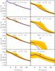 |
Fig. 6 Top: evolution of the Fe profile for stars of different ages, born in situ (dotted curves) and presently found at radius Rfin (solid); the shaded area indicates the ±1σ range of values. |
In Fig. 6 we display the evolution of the Fe profiles of our model for all the stars ever born (right bottom panel) and for stars of different age ranges. We show the average metallicity for stars formed in situ4 and for all stars found in radius r at the end of the simulation; the latter population has been affected by radial migration. It can be seen that for the younger stars (up to 4 Gyr old) the differences between the corresponding profiles is small, for two reasons: i) radial migration does not have time to shuffle stars away from their birth places; and (most importantly) ii) at late times, the abundance profile is flatter than in earlier period, so that even an efficient radial migration cannot produce a strong effect, because the abundance differences between different radii are small in any case. Still, radial migration steadily increases the dispersion in metallicity with age at all radii.
For stars older than the Sun, the effect of radial migration on the abundance profiles becomes more and more important, because it makes the profiles appear flatter today than they were at the time of the stellar birth, and flatter than the ones of younger stellar populations (even though the corresponding gaseous profile was steeper in the past). In particular, the oldest stars (presumably belonging to the thick disk) have a quasi-flat profile in the inner region, extending up to 6 kpc; beyond 9−10 kpc, however, the corresponding metallicity drops rapidly to values that are characteristic of halo stars.
The impact of radial migration on the past abundance profiles of a galactic disk was first identified by Roškar et al. (2008). In their Fig. 2 they show how the older stars of their simulation (>5 Gyr) have a quasi-flat metallicity profile throughout the disk. Although it is difficult to compare our results directly with other models of similar scope, because of the many different assumptions involved (see KPA15 for a brief description of the differences between the models of Schönrich & Binney 2009; Minchev et al. 2013; and KPA15), we attempt such a comparison here to the results of Minchev et al. (2014). In their Fig. 9 (top left), they provide results for the stellar abundances of practically all stars of their model (found at the end of the simulation within a distance of 3 kpc from the galactic plane), as function of galactocentric radius and stellar age. There are differences and similarities with our results, but it is not clear whether the latter are due to similarities in the models or to different boundary conditions. In particular, they also find that the older stars have a flatter abundance profile than the younger ones; however, this is probably due not to radial migration, but to the fact that in their case the abundance profile of gas is also flatter in early time than later times, a characteristic feature of the model of Chiappini et al. (2001). In their case, dispersion in metallicity is more important for older stars than for young ones, as in our case and probably for the same reason, i.e. more time for radial migration being available to older objects and/or larger epicyclic motions; however, this dispersion appears to extend further outwards for the younger stellar population, whereas the opposite is obtained in our case. Finally, the older stars in their simulation display a quasi-flat abundance profile over the whole disk, whereas our corresponding metallicity profiles plummet beyond 9−10 kpc. This difference is simply because we start our simulation with gas of primordial composition, whereas they adopt an initial metallicity of 0.1 Z⊙. Such differences may have negligible impact in some cases (i.e. for almost any observable concerning the solar neighbourhood), but turn out to be crucial in others.
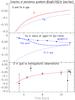 |
Fig. 7 Top: evolution of the gaseous O and Fe abundance gradients. Middle: the evolution of the gaseous Fe gradient (dotted, same as in top panel) is compared to the evolution of the stellar Fe gradient, as it appears today after stellar migration (thick dashed). The squares, connected by solid segments represent the results of Minchev et al. (2014, their Table 2), for all stars found within distance Z< 3 kpc from the galactic plane. Bottom: the evolution of the O abundance gradient in the gas (same as in top panel) is compared to the extragalactic data compiled from Jones et al. (2013). The three open symbols correspond to an evaluation of MW data, which is superseded by the recent one of Maciel & Costa (2013), who find no clear indications for any evolution of the abundance gradient. |
We show the evolution of the O and Fe abundance gradients in Fig. 7. As already discussed, gaseous gradients decrease in absolute value with time; i.e., the abundance profiles become flatter with time (at least in the framework of this type of model). Hou et al. (2000) performed the first comparison between the evolution of the O and Fe abundance gradients and found that Fe gradients are steeper than those of O − by ~0.1 dex − because of the role of SNIa: the ratio of SNIa/CCSN is larger in the inner disk than in the outer one (see Fig. 1). We confirm this result here, but we obtain a larger difference between the two gradients −~0.25 dex − because of the more efficient star formation in the inner disk and the role of radial migration: the latter increases the abundance of Fe by ~10%, but not the one of O, in the region outside 6 kpc (see bottom panels in Fig. 3).
As discussed in the previous paragraphs, radial migration modifies the presently observed evolution of stellar profiles. This is illustrated in the middle panel of Fig. 7, where the evolution of the Fe gradient in the gas is compared to the Fe gradient of stellar population as a function of their age. The gradients have been the same for the past ~2 Gyr (see also Fig. 6) but beyond that age the two curves start deviating: the one corresponding to the stellar population becomes flatter with age. For the oldest stars, the gradient is close to zero (the abundance profile is practically flat). Our results are qualitatively similar to those of Minchev et al. (2014), also displayed in Fig. 7, although the evolution is milder in their case.
It is difficult to directly compare the “age effect” of radial migration on the abundance profile to observations, because of the uncertainties in stellar age estimates. However, there is an indirect way through the fact that older stars are, on average, located farther away from the plane of the disk than younger ones, because of the increase in the vertical velocity dispersion with stellar age. Thus, analysing a sample of old, main sequence stars belonging to the thin and thick disks from the SEGUE survey, Cheng et al. (2012) find that the Fe gradient in the region 6 <r(kpc) < 16 increase from −0.065 dex kpc-1 at a vertical distance from the plane Z = 0.2 kpc to a positive value at Z> 1 kpc. This is a clear signature of older stellar populations having flatter abundance profiles, as found in Roškar et al. (2008), Minchev et al. (2014) and in this work. However, our model lacks the vertical dimension to the galactic plane, so we cannot compare directly to the data of Cheng et al. (2012). At each distance from the plane there is a mixture of stellar populations, and the contributions of older stars increase with that distance. Our results presented in Fig. 7 (middle panel) include all stars found today between galactocentric radii of 4 and 11 kpc. Qualitatively, they agree with the observations, since they suggest a gradient close to nought for the oldest stars and close to −0.07 dex/kpc for the youngest ones. A detailed comparison to the observations would require a model including the z dimension (vertical to the plane), including the observational biases, i.e. slices at appropriate distances from the plane, as in Minchev et al. (2014). Alternatively, such a comparison would be possible if a volume-limited sample with accurate stellar ages were available.
The bottom panel of Fig. 7 illustrates another way of comparing model results to observations of abundance gradient evolution. The results concern the evolution of the oxygen abundance gradient in the gas (as in top panel). The data are from observations of oxygen in high-redshift lensed disk galaxies, from the recent compilation of Jones et al. (2013); they find that the metallicity gradients flatten with time, by a factor of 2.6 ± 0.9, on average, between redshifts 2.2 and 0, although they acknowledge that the discrepancy with the MASSIV data − the highest data point in the bottom panel of Fig. 7− warrants further investigation. Barring that puzzling discrepancy, we find rather fair agreement of the high redshift data with our results. It should be stressed, however, that the comparison may not be meaningful after all, because its not clear whether those isolated high redshift systems are progenitors of MW-like disks.
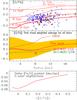 |
Fig. 8 Top: evolution of the O/Fe profile. Data are for Cepheids (filled circles, from Luck & Lambert 2011) and for open clusters (Yong et al. 2012, asterisks and Frinchaboy et al. 2013, squares). Dotted curves correspond to model stars of average ages 11, 8, 4 and 0.2 Gyr (from top to bottom) formed in situ and solid curves to stellar populations of the same age found today at radius r. Middle: mass-weighted stellar [O/Fe] profile vs. radius. The solid red curve indicates our results and the shaded area the corresponding ±1σ range. The dashed curves are from Fig. 2 of Gibson et al. (2013) and indicate results of Schönrich & Binney (2009) and Gibson et al. (2013), the latter obtained with two different models (see text). Bottom: the stellar Fe/H gradient of stars found today in the region 5−11 kpc is plotted vs. the average [O/Fe] ratio of those stars (see text). |
3.4. O/Fe profile
The variation in the O/Fe ratio provides important information on the evolutionary status of a galactic system: high O/Fe values (typically ~3 times solar) indicate a chemically young system, enriched only by the ejecta of CCSN, while close to solar values indicate systems that are several Gyr old, also enriched by SNIa. The transition from high O/Fe (and, more generally, high α/Fe) to low O/Fe values constitutes one of the key tracers of the chemical evolution of the local Galaxy (the halo-to-disk transition) and of nearby dwarf galaxies as well.
In the case of the MW disk,the O/Fe ratio is expected to vary, from high values in the “young” outer disk to lower ones in the older inner disk, in the framework of the inside-out formation scheme. In Fig. 8 (top panel), we plot the O/Fe radial profile for stellar populations of various ages, for all the stars found in a given region in the end of the simulation, and for stars formed in situ. The decrease (with time) of O/Fe occurs first in the inner galaxy and progressively moves outwards. The youngest objects have [ O / Fe ] ~ 0.1 in the outer disk and ~−0.25 in the innermost regions, whereas the ratio varies from 0.5 to 0.4 for the oldest objects. As in the case of the Fe/H profile, radial migration modifies the O/Fe profiles by bringing evolved stellar populations (of lower O/Fe) into outer regions; the effect is more important for the oldest stars and affects the region between 4 and 12 kpc.
Similar results, at least qualitatively, appear in Fig. 9 (bottom left panel) of Minchev et al. (2014), where the [Mg/Fe] profile is plotted for stars of different ages. Since Mg is an α element, a comparison to the O/Fe profile is meaningful5. They obtain a variation in [Mg/Fe] for their youngest stars ranging from ~−0.16 at r = 6 kpc to ~0.1 at r = 16 kpc, as well as a flat Mg/Fe profile for the oldest stars; both results are in fair agreement with ours.
Figure 8 (top panel) displays observational data from Cepheids and open clusters of various ages. As with the corresponding Fe/H profile of Fig. 5, the dispersion in the O/Fe ratio at every galactocentric radius is quite large and cannot be explained with our models; radial migration can only play a marginal role in that respect for such young objects. No clear trend with radius appears in the case of Cepheids, while the data for open clusters are marginally consistent with such a trend, as discussed in Yong et al. (2012).
In the middle panel of Fig. 8, we plot the results for the mass-weighted average of all stars at the end of our simulation. We obtain a rather flat profile in the inner disk. The average [ O / Fe ] ~ 0.1 in that region corresponds to stars older than 8 Gyr, as inferred through a comparison to the upper panel, which have been mixed throughout the inner disk by radial migration. In the outer disk, which is less affected by radial migration, the average [O/Fe] ratio increases slowly but steadily, up to a value of 0.2. The overall 1σ dispersion is much larger in the inner disk than in the outer one. We compare our results to the corresponding ones reported in Fig. 2 of Gibson et al. (2013) and reproduced in the middle panel of our Fig. 8. The semi-analytical model of Schönrich & Binney (2009) displays a much steeper slope of [O/Fe] vs. radius, which may result from less radial mixing than in our case or from a much larger gradient of stars formed in situ. We think that both reasons contribute to the difference with our results, considering that Schönrich & Binney (2009) obtain quite large Fe gradients (dlog (Fe / H) / dr ~−0.1 dex kpc-1) and that they consider radial mixing that is induced only by the transient spiral mechanism of Sellwood & Binney (2002) and not by the more efficient bar-spiral interaction of our model. On the other hand, both models of Gibson et al. (2013) display a very flat profile of [O/Fe] over the whole disk, which is rather difficult to understand in view of the enhanced SNIa/CCSN ratio in the inner disk expected from inside-out formation schemes (as discussed in Sect. 2), unless if a very efficient radial mixing occurs for the stars over the whole disk. It is clear, however, that for different reasons, which have not necessarily been analysed well yet, different models make different predictions for the profiles of metallicity and of various abundance ratios and only observations will help clarify the situation.
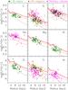 |
Fig. 9 Abundance profiles from C to Ar and comparison to data from PN (magenta triangles), B-stars (green squares) and HII-regions (brown dots); data sources are provided in Table 1. Model curves correspond to gaseous profiles at time 4, 8 and 12 Gyr (thick), respectively. |
Finally, the bottom panel of Fig. 8 illustrates another use of the O/Fe ratio to probe the evolution of the Galactic disk. As found in KPA15, the O/Fe ratio declines monotonically with time and displays very little dispersion from radial mixing at any age. It constitutes thus a natural “chronometer” as argued in Bovy et al. (2012) and it can be used in cases where stellar ages are not known or accurately measured. Toyouchi & Chiba (2014) have analysed 18500 disk stars from the SDSS and HARPS surveys and plotted the Fe/H gradients as a function of the [α/Fe] values of the corresponding stellar populations. They find that, starting with the youngest stars (lowest [α/Fe] values), the gradient first decreases (it becomes more negative) and then increases, reaching positive values. However, they find large systematic differences between the samples of the two surveys (concerning the absolute values of the gradients and the turning points in [α/Fe]). We display our results in the bottom panel of Fig. 8, showing qualitative agreement with the findings of Toyouchi & Chiba (2014). Starting with the youngest stars, the Fe/H gradient first shows a small decline, as slightly older stellar populations are probed (with a steeper Fe gradient because too young to be affected by radial migration); then, older populations are probed, more and more affected by radial migration and displaying flatter Fe/H profiles (as also indicated in the middle panel of our Fig. 7). The oldest stars have a nearly flat Fe/H profile, but we never find a positive gradient, as Toyouchi & Chiba (2014) do. We stress again that a meaningful comparison to observations should involve models properly accounting for observational biases.
3.5. Other elements
Oxygen and iron are the most frequently observed elements in the solar neighbourhood and the MW disk. Their abundances (as a function of time and/or space) constitute important constraints on the chemical evolution of the Galaxy. The other elements play a marginal role in that respect: their observations mainly serve to support conclusions obtained through the observations of O and Fe or to constrain stellar nucleosynthesis models.
In Fig. 9 we present our results for eight more elements, with abundance profiles derived from observations of B stars, HII regions and planetary nebulae. In most cases, available data are for the region 4−12 kpc, with the exceptions of N and S (and, of course, O) where observations of H-II regions and PN extend up to 17 kpc. The inclusion of PN, presumably covering a wide range of ages, increases the dispersion considerably at every radius.
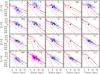 |
Fig. 10 Abundance profiles from C to Zn and comparison to Cepheid data (from Luck & Lambert 2011; except for Fe data, provided in Genovali et al. 2014). Model curves correspond to the gaseous profiles after 4, 8 and 12 (thick curve) Gyr, respectively. |
Among the nine elements of Fig. 9, those heavier than N are almost exclusively products of massive stars; Si and heavier elements receive a small, but non-negligible contribution from SNIa, which we take into account through the adopted yields of SNIa from Iwamoto et al. (1999). All those elements are produced as “primaries”; i.e., their stellar yields depend little on the initial metallicity of the stars. C and N have a complex nucleosynthetic origin, since they are produced both by massive and and intermediate mass stars. Their yields from massive stars are sensitive to still poorly understood (and metallicity-dependent) stellar properties, such as mass loss and rotation. In lower mass stars, C is produced in the shell He-burning of the asymptotic giant branch (AGB) phase and ejected in the ISM through the 3d dredge-up, while N may be produced in the bottom of the convective envelope of the AGB star (“hot-bottom burning”) at the expense of C. N is, in principle, a “secondary” element (being synthesized from the initial C and O during the CNO cycle, its yield depends on the initial metallicity); however, it may be also produced as primary in the “hot-bottom burning” of intermediate mass asymptotic giant branch (AGB) stars and in fast-rotating massive stars.
The yields from Nomoto et al. (2013) that we adopted in this work include yields from low mass stars from Karakas (2010), but the ones for massive star concern non-rotatings stars. Given the complexity of the nucleosynthesis of C and N, we consider that a dedicated study for the evolution of those two elements would be necessary, so we do not attempt it here.
The results displayed in Fig. 9 present similar features to those already discussed for O, namely a flattening of the abundance profiles with time (due to the inside-out formation) and a slightly hollow profile in the bar region at late times (due to the combined action of the bar and of metal-poor infall). Available data, however, display either differences that are too large (e.g. between B-stars and PN for S) or dispersion that is too large (in the case of PN data), or else they are too scarce (e.g. for C) to allow for any serious constrains, either on the model or on the yields (Fig. 7, middle panel)
In Fig. 10 we compare our results for all elements between C and Ni to a homogeneous data set for Cepheids (Luck & Lambert 2011), which is large enough for a statistically meaningful comparison with models. Still, Cepheids are relatively massive (>3 M⊙) and evolved stars, having gone through the first dredge-up. This implies that they are expected to exhibit large amounts of N at their surface, formed in situ at the expense of C, and perhaps of O; Na is also possibly affected by H-burning in those stars. In consequence, none of those four elements observed in Cepheids can be used as tracer of the chemical evolution of the Galaxy (but they may certainly be used as probes of the internal nucleosynthesis of Cepheids).
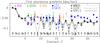 |
Fig. 11 Present day abundance gradients from H to Ni: models vs. observations. Observations are from H-II regions (Rudolph et al. 2006), B-stars (Daflon & Cunha 2004), Planetary nebulae (Henry et al. 2004) and Cepheids (Luck & Lambert 2011; Luck et al. 2011; Lemasle et al. 2013). Model results are obtained with the model described here and three different sets of yields, from Nomoto et al. (2013), Woosley & Weaver (1995) and Chieffi & Limongi (2004), as indicated by the open symbols and discussed in the text. |
Concerning the other elements, one sees that observed abundances are systematically higher than solar in the solar neighbourhood (except for Mn and Ni), in rough agreement with theoretical expectations. Our final abundance profiles are globally in agreement with the data, although the obtained slope is, in general, slightly larger than the observationally inferred one, as we discuss below. Finally, the Cepheid data do not extend into the bar region, as to allow us to probe the predictions of the model there.
In Fig. 11, we present a quantitative comparison of the gradients of all elements between H and Ni to the data set of Cepheids from Luck & Lambert (2011), complemented by a few other data presented here for completeness. We notice, however, that the abundance profiles are not necessarily perfect exponentials to be fit by straight lines of a single slope in logarithmic space. In our case they are not, and the slope depends on the radial range considered: here we take the range 4−17 kpc, to compare directly with the slopes provided by Luck & Lambert (2011) for that same range. The other data sets correspond, however, to different radial ranges, making a direct comparison difficult.
To have an idea of the theoretical uncertainties, we provide results for three runs of the same model using three different sets of yields. The first one is from Nomoto et al. (2013; mass range for massive stars: 13−40 M⊙) using the low-mass yields of Karakas (2010; 1−6 M⊙), as discussed throughout this work. The second set adopts the massive star yields of Woosley & Weaver (1995; 12−40 M⊙) and the ones of van den Hoek & Groenewegen (1997; 0.9−8 M⊙) for intermediate mass stars. The third one adopts the massive star yields of Chieffi & Limongi (2004; 13−35 M⊙) and those of van den Hoek & Groenewegen (1997) for intermediate mass stars. All those yields are metallicity-dependent, but they cover different ranges of masses and metallicities.
The limited cover of the mass grid by all the data sets implies the need for interpolation between the low-mass and massive star ranges, and extrapolation between the most massive star of the calculated yields and the most massive star of the adopted IMF, here taken to be 100 M⊙. These operations introduce numerical biases into the results. For the metallicities, the yields of Nomoto et al. (2013) are provided for a finer grid and extend to supersolar metallicities, with both features essential for a consistent study of the evolution of the MW disk. The calculations of massive stars involve different ingredients, e.g. no mass loss in Woosley & Weaver (1995) and Chieffi & Limongi (2004) vs. mass loss in Nomoto et al. (2013), different prescriptions for some key nuclear reaction rates or the various mixing mechanisms and the description of the final supernova explosion.
Similar differences characterise the physics underlying the yields of intermediate mass stars, for example, the treatment of hot-bottom burning. Those differences, as well as other important ingredients (not considered in those calculation, like e.g. rotation) make any attempt for a systematic comparison between sets of yields rather futile. We provide such a comparison only for illustrative purposes, and he reader should be aware that the overall theoretical uncertainties should be larger than found here. We simply notice that, in all cases we keep the same IMF and the same prescription for the rate and yields of SNIa.
An inspection of Fig. 11 shows that the observed gradients of all elements between C and Ni lie in the narrow range of dlog X / dr ~−0.04 to −0.06 dex kpc-1, with the exception of C and (curiously) S. Taking the larger error bars into account, the data for other tracers are in good agreement with those of Cepheids.
Theoretical results present some features that are common to all sets of adopted yields.
-
i)
quasi-identical slopes for the Fe-peak elements, dominated bySNIa;
-
ii)
quasi-identical slopes for all α-elements beyond Ne;
-
iii)
a distinctive difference in the slopes of even vs. odd elements, the former being smaller in absolute value than the latter. To our knowledge, it is the first time that the “odd-even” effect of nucleosynthesis, known to affect the behaviour of the abundance ratios in low metallicity stars (e.g. Goswami & Prantzos 2000), is put in evidence in the case of the Galactic abundance gradients.
-
The yields of Nomoto et al. (2013) produce flatter profiles for C, N and O than those of Woosley & Weaver (1995) or Chieffi & Limongi (2004). We find that this is due mainly to the impact of the yields of low-mass stars (from Karakas 2010 in the former case), which have more pronounced “hot-bottom burning” than the yields of van den Hoek & Groenewegen (1997) adopted in the last two cases.
-
The “odd-even” effect appears to be more pronounced with the yields of Woosley & Weaver (1995) than with those of Nomoto et al. (2013), and even more so with the yields of Chieffi & Limongi (2004).
-
F is a particular case, since Woosley & Weaver (1995) and Nomoto et al. (2013) include the effect of ν-induced nucleosynthesis during the final SN explosion, while Chieffi & Limongi (2004) do not.
Comparing model results to observations, one sees a significant offset of the former − by ~0.02 dex downwards − for all elements beyond Cl except Fe. For lighter elements, there is satisfactory agreement (within error bars) for the even elements, but significant discrepancy for the odd ones.
Some conclusions may be drawn from the comparison between model and observations on the one hand, and between different sets of yields on the other. First, if the systematic discrepancy of ~0.01−0.02 dex between model results and observations is confirmed, some key ingredients of the model should be revised: this could be the case, for instance, of the timescales of the infall rate, which should be lower in the outer disk than adopted here (as to favour a more rapid evolution and larger final abundances in that region); alternatively, a metal-enriched composition of the infalling gas could be adopted, instead of the primordial one adopted here. We find, however, that in the framework of this model the required infall metallicity is ~0.4 Z⊙, too large for the infalling gas (acceptable metallicities, up to 0.2 Z⊙, increase the slope by only 0.01 dex/kpc). Second, it is interesting to see whether the abundance gradients present any systematic trends with the atomic number of the element, i.e. either steeper profiles for Fe-peak elements or the “odd-even” effect. If this turns out not to be the case, then the yields of nucleosynthesis should be revised and the role of the IMF scrutinized (because more massive stars produce larger ratios of α/Fe). In any case, the abundance profiles of a large number of elements should be accurately established, on as large a radial basis as possible. Then, the abundance profiles could be used to probe stellar nucleosynthesis, a role played already by abundance ratios in low metallicity halo stars.
We notice that the study of Romano et al. (2010), concerning the impact of different sets of yields on the chemical evolution of the MW, reaches conclusions that present similarities to our own, but also some differences. Their model has no radial migration or radial inflows and uses different prescriptions for the SFR and infall rate than ours; thus, they obtain different abundance profiles, flatter than ours by ~0.02 dex/kpc for C and O (their Fig. 17 left). Still, they adopt the same IMF, while their Models 1 and 15 adopt similar sets of yields with our study. The former adopts Woosley & Weaver (1995) for massive stars and van den Hoek & Groenewegen (1997) for low and intermediate mass stars (LIMS), while the latter uses the yields of Nomoto et al. (2013) which include those of Karakas (2010) for LIMS. Thus, some comparison with our results becomes possible. Romano et al. (2010) find that “... for some elements, different choices for the yields provide also different slopes for the gradients; this is the case for carbon and oxygen, while a negligible effect is seen for other elements, including those heavier than Si”. We confirm the case for C and O, but attribute it to the differences in the corresponding yields of LIMS, while Romano et al. (2010) attribute it to the yields of rotating, massive stars with mass loss.We did not study that case here. On the other hand, we confirm that the impact on the slope of the abundance profiles is negligible for other even elements, but we find a significant effect for the odd elements, as we emphasized in the previous paragraphs.
4. Summary
In this work we studied the abundance profiles of elements between H and Ni in the MW disk, using a semi-analytical model that inncludes the radial motions of gas and stars. We adopted parametrised descriptions of those radial motions, which are based on N-body simulations for the case of stars and on a simple analytical prescription for the gas radial velocity profile and are inspired by the presence of a bar in the Milky Way. Other key ingredients of the model is the assumption of a SFR dependent on the molecular gas and the use of a fine grid of recent stellar yields from Nomoto et al. (2013), which include up-dated yields of low-mass stars from Karakas (2010) and cover a wide range of initial metallicities. The model successfully reproduces a large number of observations concerning the solar neighbourhood and the disk of the MW, as discussed in KPA15. They include the local age-metallicity relation and metallicity distribution, the α/Fe vs. Fe/H relation and the surface density profiles of the thin and thick disks, as well as the profiles of stars, SFR, HI and H2, and the total amounts of gas, stars, SFR, CCSN and SNIa rates in the disk and the bulge of the MW.
In Sect. 2 we presented the key model ingredients and showed how the radial motions affect the profiles of stars, gas, SFR, SNIa and Fe. We found that the effect mainly concerns the inner disk, because of the key role played by the Galactic bar in radial migration according to our assumptions. Its effect on the disk was found to be negligible beyond 12 kpc, with the adopted prescriptions. The effect on the Fe profile in the inner disk is rather small (of the order of 10% and it is due to the role of SNIa from long-lived progenitors, which have enough time to migrate away from their birth place.
In Sect. 3 we presented our results and compared them to a large number of observational data from various metallicity tracers (H-II regions, B-stars, PN, Cepheids and open clusters). We notice that the data base is not homogeneous and does not cover the radial extent of the MW disk uniformly.
Our abundance profiles cannot be characterised by a unique slope, since they flatten progressively towards the outer disk (as a result of the adopted SFR prescription) and towards the inner disk (as a result of the radial flow induced by the bar). We found that the abundance profiles flatten with time, as a result of the inside-out formation of the disk. But the observational confirmation of this effect in the MW becomes impossible because of the effect of radial migration, which cancels and even inverts it. We confirmed (Sect. 3.3) the main effect of radial migration on the abundance profiles found by Roškar et al. (2008), namely the flattening of the past abundance profiles of stars, which becomes more pronounced for the older stellar populations. We quantitatively compared our results (Fig. 7, middle panel) to those of Minchev et al. (2014), who find similar, albeit somewhat flatter, abundance profiles.
The evolution of our gaseous abundance profiles is in fair agreement with the extragalactic, high redshift, data compiled by Jones et al. (2013), which are too uncertain at present, however, to draw firm conclusions (Fig. 7, bottom panel). In Sect. 3.4 we present the evolution of our [O/Fe] profiles. The evolution of both [Fe/H] and [O/Fe] profiles, modified by radial migration, is encoded in the stellar populations currently present in the local disk and is revealed by preliminary observations of those quantities in stars at different distances from the plane of the disk. Our 1D model lacks the dimension vertical to the plane that would allow us to perform a meaningful comparison to such observations, but the results discussed in Sect. 3.4 are in qualitative agreement with the data. (The profiles are expected to flatten with distance from the plane.)
In Sect. 3.5 we present our results for all elements between C and Ni. From the theoretical point of view, we stressed the systematic differences in the final abundance profiles due to the different sets of stellar yields (the physics of both low and high mass stars still suffering from several uncertainties). We found rather good agreement with observationally derived slopes of abundance profiles (assuming they can be described by a single exponential) but also some systematic differences (see Fig. 11: in particular, we obtained slopes that are systematically 0.01−0.02 dex larger (in absolute value) than the observed ones). We argued that this difference, if definitively established, could be cured by some revision of basic ingredients in the model, namely the need for smaller infall timescales in the outer disk or a non-primordial composition for the infalling gas. We also find an interesting “odd-even” effect of larger slopes for odd elements. This metallicity-dependent effect, already discussed in the context of abundance ratios X/Fe in halo stars, is found here for the first time and is generic, i.e. it concerns all sets of stellar yields. However, it does not appear in the observational data; if observations are confirmed, then some of the stellar nucleosynthesis results should be revised.
The composition of the infall is equally important when it comes to discussing the evolution of abundances and abundance ratios in the MW disk. Observations are of little help at present because they generally find low metallicities for gas clouds presently falling to the MW disk (~0.1 Z⊙, e.g. Wakker et al. 1999), but they provide no information on the past metallicity of such clouds or on their abundance ratios. Here we adopt the simplest possible assumption, namely that the infalling gas always has primordial composition. This assumption hardly affects the results for the chemical evolution of the disk, but it allows for the existence of disk stars with metallicities lower than [ Fe / H ] = −1 (see Bensby 2014, and references therein).
For each “birth radius” there are approximately as many stars migrating outwards as inwards. However, there are more stars in the inner regions than in the outer ones, because of the exponentially declining outwards surface density profile. As a result, the outer regions receive more stars from the inner ones than what they send to them: the radial profile of the fraction of stars that each region receives from the others is not symmetric but biased towards the inner regions, i.e. each disk annulus receives more stars from the inner regions than from the outer ones.
![\hbox{$<[{\rm Z/H}]>=\frac{\Sigma N_i[{\rm Z/H}]_i}{\Sigma N_i}$}](/articles/aa/full_html/2015/08/aa24599-14/aa24599-14-eq65.png)
Acknowledgments
We are grateful to an anonymous referee for the constructive report. E.A. acknowledges financial support to the DAGAL network from the People Programme (Marie Curie Actions) of the European Union’s Seventh Framework Programme FP7/2007-2013/ under REA grant agreement number PITN-GA-2011-289313 and from the CNES (Centre National d’Études Spatiales − France). We also acknowledge partial support from the PNCG (Programme National Cosmologie et Galaxies − France).
References
- Adibekyan, V. Z., Santos, N. C., Sousa, S. G., & Israelian, G. 2011, A&A, 535, L11 [NASA ADS] [CrossRef] [EDP Sciences] [Google Scholar]
- Asplund, M., Grevesse, N., Sauval, A. J., & Scott, P. 2009, ARA&A, 47, 481 [NASA ADS] [CrossRef] [Google Scholar]
- Athanassoula, E. 1992, MNRAS, 259, 345 [NASA ADS] [CrossRef] [Google Scholar]
- Bensby, T. 2014, IAU Symp., 298, 17 [NASA ADS] [Google Scholar]
- Bensby, T., Feltzing, S., & Oey, M. S. 2014, A&A, 562, A71 [NASA ADS] [CrossRef] [EDP Sciences] [Google Scholar]
- Bilitewski, T., & Schönrich, R. 2012, MNRAS, 426, 2266 [NASA ADS] [CrossRef] [Google Scholar]
- Blitz, L., & Rosolowsky, E. 2006, ApJ, 650, 933 [NASA ADS] [CrossRef] [Google Scholar]
- Blitz, L., & Spergel, D. N. 1991, ApJ, 379, 631 [NASA ADS] [CrossRef] [Google Scholar]
- Boissier, S., & Prantzos, N. 1999, MNRAS, 307, 857 [NASA ADS] [CrossRef] [Google Scholar]
- Boissier, S., & Prantzos, N. 2009, A&A, 503, 137 [NASA ADS] [CrossRef] [EDP Sciences] [Google Scholar]
- Bovy, J., & Rix, H.-W. 2013, ApJ, 779, 115 [NASA ADS] [CrossRef] [Google Scholar]
- Bovy, J., Rix, H.-W., Liu, C., et al. 2012, ApJ, 753, 148 [NASA ADS] [CrossRef] [Google Scholar]
- Brunetti, M., Chiappini, C., & Pfenniger, D. 2011, A&A, 534, A75 [NASA ADS] [CrossRef] [EDP Sciences] [Google Scholar]
- Cavichia, O., Mollá, M., Costa, R. D. D., & Maciel, W. J. 2014, MNRAS, 437, 3688 [NASA ADS] [CrossRef] [Google Scholar]
- Chamcham, K., & Tayler, R. J. 1994, MNRAS, 266, 282 [NASA ADS] [CrossRef] [Google Scholar]
- Cheng, J. Y., Rockosi, C. M., Morrison, H. L., et al. 2012, ApJ, 746, 149 [NASA ADS] [CrossRef] [Google Scholar]
- Chiappini, C. 2009, in IAU Symp. 254, eds. J. Andersen, B. M., Nordströara, & J. Bland-Hawthorn, 191 [Google Scholar]
- Chiappini, C., Matteucci, F., & Gratton, R. 1997, ApJ, 477, 765 [NASA ADS] [CrossRef] [Google Scholar]
- Chiappini, C., Matteucci, F., & Romano, D. 2001, ApJ, 554, 1044 [NASA ADS] [CrossRef] [Google Scholar]
- Chiappini, C., Górny, S. K., Stasińska, G., & Barbuy, B. 2009, A&A, 494, 591 [NASA ADS] [CrossRef] [EDP Sciences] [Google Scholar]
- Chieffi, A., & Limongi, M. 2004, ApJ, 608, 405 [NASA ADS] [CrossRef] [Google Scholar]
- Clarke, C. J. 1989, MNRAS, 238, 283 [NASA ADS] [CrossRef] [Google Scholar]
- Daflon, S., & Cunha, K. 2004, ApJ, 617, 1115 [NASA ADS] [CrossRef] [Google Scholar]
- Dutil, Y., & Roy, J.-R. 1999, ApJ, 516, 62 [NASA ADS] [CrossRef] [Google Scholar]
- Edmunds, M. G., & Greenhow, R. M. 1995, MNRAS, 272, 241 [NASA ADS] [CrossRef] [Google Scholar]
- Ferrini, F., Molla, M., Pardi, M. C., & Diaz, A. I. 1994, ApJ, 427, 745 [NASA ADS] [CrossRef] [Google Scholar]
- Friedli, D., & Benz, W. 1993, A&A, 268, 65 [NASA ADS] [Google Scholar]
- Friedli, D., Benz, W., & Kennicutt, R. 1994, ApJ, 430, L105 [NASA ADS] [CrossRef] [Google Scholar]
- Frinchaboy, P. M., Thompson, B., Jackson, K. M., et al. 2013, ApJ, 777, L1 [NASA ADS] [CrossRef] [Google Scholar]
- Genovali, K., Lemasle, B., Bono, G., et al. 2014, A&A, 566, A37 [NASA ADS] [CrossRef] [EDP Sciences] [Google Scholar]
- Gibson, B. K., Pilkington, K., Brook, C. B., Stinson, G. S., & Bailin, J. 2013, A&A, 554, A47 [NASA ADS] [CrossRef] [EDP Sciences] [Google Scholar]
- Goetz, M., & Koeppen, J. 1992, A&A, 262, 455 [NASA ADS] [Google Scholar]
- Goswami, A., & Prantzos, N. 2000, A&A, 359, 191 [NASA ADS] [Google Scholar]
- Greggio, L. 2005, A&A, 441, 1055 [NASA ADS] [CrossRef] [EDP Sciences] [Google Scholar]
- Guesten, R., & Mezger, P. G. 1982, Vistas Astron., 26, 159 [NASA ADS] [CrossRef] [Google Scholar]
- Gummersbach, C. A., Kaufer, A., Schaefer, D. R., Szeifert, T., & Wolf, B. 1998, A&A, 338, 881 [NASA ADS] [Google Scholar]
- Hamuy, M. 2003, ArXiv e-prints [arXiv:astro-ph/0301006] [Google Scholar]
- Heiter, U., Soubiran, C., Netopil, M., & Paunzen, E. 2014, A&A, 561, A93 [NASA ADS] [CrossRef] [EDP Sciences] [Google Scholar]
- Henry, R. B. C., Kwitter, K. B., & Balick, B. 2004, AJ, 127, 2284 [NASA ADS] [CrossRef] [Google Scholar]
- Henry, R. B. C., Kwitter, K. B., Jaskot, A. E., et al. 2010, ApJ, 724, 748 [NASA ADS] [CrossRef] [MathSciNet] [Google Scholar]
- Hou, J. L., Prantzos, N., & Boissier, S. 2000, A&A, 362, 921 [NASA ADS] [Google Scholar]
- Iwamoto, K., Brachwitz, F., Nomoto, K., et al. 1999, ApJS, 125, 439 [NASA ADS] [CrossRef] [MathSciNet] [Google Scholar]
- Jones, T., Ellis, R. S., Richard, J., & Jullo, E. 2013, ApJ, 765, 48 [NASA ADS] [CrossRef] [Google Scholar]
- Karakas, A. I. 2010, MNRAS, 403, 1413 [NASA ADS] [CrossRef] [Google Scholar]
- Kroupa, P. 2002, Science, 295, 82 [NASA ADS] [CrossRef] [PubMed] [Google Scholar]
- Kubryk, M., Prantzos, N., & Athanassoula, E. 2013, MNRAS, 436, 1479 [NASA ADS] [CrossRef] [Google Scholar]
- Kubryk, M., Prantzos, N., & Athanassoula, L. 2015, A&A, 580, A126 [NASA ADS] [CrossRef] [EDP Sciences] [Google Scholar]
- Lacey, C. G., & Fall, S. M. 1985, ApJ, 290, 154 [NASA ADS] [CrossRef] [Google Scholar]
- Lemasle, B., François, P., Genovali, K., et al. 2013, A&A, 558, A31 [NASA ADS] [CrossRef] [EDP Sciences] [Google Scholar]
- Li, Y., Mo, H. J., van den Bosch, F. C., & Lin, W. P. 2007, MNRAS, 379, 689 [NASA ADS] [CrossRef] [Google Scholar]
- Loebman, S. R., Roškar, R., Debattista, V. P., et al. 2011, ApJ, 737, 8 [NASA ADS] [CrossRef] [Google Scholar]
- Luck, R. E., & Lambert, D. L. 2011, AJ, 142, 136 [NASA ADS] [CrossRef] [Google Scholar]
- Luck, R. E., Andrievsky, S. M., Kovtyukh, V. V., Gieren, W., & Graczyk, D. 2011, AJ, 142, 51 [NASA ADS] [CrossRef] [Google Scholar]
- Maciel, W. J., & Costa, R. D. D. 2009, in IAU Symp. 254, eds. J. Andersen, Nordströara, B. M., & J. Bland-Hawthorn, 38 [Google Scholar]
- Maciel, W. J., & Costa, R. D. D. 2013, Rev. Mex. Astron. Astrofis., 49, 333 [NASA ADS] [Google Scholar]
- Magrini, L., Sestito, P., Randich, S., & Galli, D. 2009, A&A, 494, 95 [NASA ADS] [CrossRef] [EDP Sciences] [Google Scholar]
- Maoz, D., Mannucci, F., & Brandt, T. D. 2012, MNRAS, 426, 3282 [NASA ADS] [CrossRef] [Google Scholar]
- Martel, H., Kawata, D., & Ellison, S. L. 2013, MNRAS, 431, 2560 [NASA ADS] [CrossRef] [Google Scholar]
- Martin, P., & Roy, J.-R. 1994, ApJ, 424, 599 [NASA ADS] [CrossRef] [Google Scholar]
- Matteucci, F., Franco, J., Francois, P., & Treyer, M.-A. 1989, Rev. Mex. Astron. Astrofis., 18, 145 [NASA ADS] [Google Scholar]
- Minchev, I., & Famaey, B. 2010, ApJ, 722, 112 [NASA ADS] [CrossRef] [Google Scholar]
- Minchev, I., Famaey, B., Quillen, A. C., et al. 2012, A&A, 548, A127 [NASA ADS] [CrossRef] [EDP Sciences] [Google Scholar]
- Minchev, I., Chiappini, C., & Martig, M. 2013, A&A, 558, A9 [NASA ADS] [CrossRef] [EDP Sciences] [Google Scholar]
- Minchev, I., Chiappini, C., & Martig, M. 2014, A&A, 572, A92 [NASA ADS] [CrossRef] [EDP Sciences] [Google Scholar]
- Mayor, M., & Vigroux, L. 1981, A&A, 98, 1 [NASA ADS] [Google Scholar]
- Mott, A., Spitoni, E., & Matteucci, F. 2013, MNRAS, 435, 2918 [NASA ADS] [CrossRef] [Google Scholar]
- Naab, T., & Ostriker, J. P. 2006, MNRAS, 366, 899 [NASA ADS] [CrossRef] [Google Scholar]
- Nomoto, K., Kobayashi, C., & Tominaga, N. 2013, ARA&A, 51, 457 [NASA ADS] [CrossRef] [Google Scholar]
- Pilkington, K., Few, C. G., Gibson, B. K., et al. 2012, A&A, 540, A56 [NASA ADS] [CrossRef] [EDP Sciences] [Google Scholar]
- Portinari, L., & Chiosi, C. 2000, A&A, 355, 929 [NASA ADS] [Google Scholar]
- Prantzos, N., & Aubert, O. 1995, A&A, 302, 69 [NASA ADS] [Google Scholar]
- Prantzos, N., & Boissier, S. 2000, MNRAS, 313, 338 [NASA ADS] [CrossRef] [Google Scholar]
- Prantzos, N., Aubert, O., & Audouze, J. 1996, A&A, 309, 760 [NASA ADS] [Google Scholar]
- Romano, D., Karakas, A. I., Tosi, M., & Matteucci, F. 2010, A&A, 522, A32 [NASA ADS] [CrossRef] [EDP Sciences] [Google Scholar]
- Roškar, R., Debattista, V. P., Quinn, T. R., Stinson, G. S., & Wadsley, J. 2008, ApJ, 684, L79 [NASA ADS] [CrossRef] [Google Scholar]
- Rudolph, A. L., Fich, M., Bell, G. R., et al. 2006, ApJS, 162, 346 [NASA ADS] [CrossRef] [Google Scholar]
- Sánchez, S. F., Rosales-Ortega, F. F., Marino, R. A., et al. 2012, A&A, 546, A2 [NASA ADS] [CrossRef] [EDP Sciences] [Google Scholar]
- Schönrich, R., & Binney, J. 2009, MNRAS, 396, 203 [NASA ADS] [CrossRef] [Google Scholar]
- Sellwood, J., & Binney, J. 2002, MNRAS, 336, 785 [NASA ADS] [CrossRef] [Google Scholar]
- Shlosman, I., & Noguchi, M. 1993, ApJ, 414, 474 [NASA ADS] [CrossRef] [Google Scholar]
- Sommer-Larsen, J., & Yoshii, Y. 1990, MNRAS, 243, 468 [NASA ADS] [Google Scholar]
- Spitoni, E., & Matteucci, F. 2011, A&A, 531, A72 [NASA ADS] [CrossRef] [EDP Sciences] [Google Scholar]
- Stanghellini, L., & Haywood, M. 2010, ApJ, 714, 1096 [NASA ADS] [CrossRef] [Google Scholar]
- Stasińska, G., Prantzos, N., Meynet, G., et al., 2012, in Oxygen in the Universe, EAS Pub. Ser., 54, 1 [Google Scholar]
- Sygnet, J. F., Tagger, M., Athanassoula, E., & Pellat, R. 1988, MNRAS, 232, 733 [NASA ADS] [CrossRef] [Google Scholar]
- Tinsley, B. M., & Larson, R. B. 1978, ApJ, 221, 554 [NASA ADS] [CrossRef] [Google Scholar]
- Tosi, M. 1988, A&A, 197, 33 [NASA ADS] [Google Scholar]
- Toyouchi, D., & Chiba, M. 2014, ApJ, 788, 89 [Google Scholar]
- van den Hoek, L. B., & Groenewegen, M. A. T. 1997, A&AS, 123, 305 [NASA ADS] [CrossRef] [EDP Sciences] [Google Scholar]
- Wakker, B. P., Howk, J. C., Savage, B. D., et al. 1999, Nature, 402, 388 [NASA ADS] [CrossRef] [PubMed] [Google Scholar]
- Woosley, S. E., & Weaver, T. A. 1995, ApJS, 101, 181 [NASA ADS] [CrossRef] [Google Scholar]
- Yong, D., Carney, B. W., & Friel, E. D. 2012, AJ, 144, 95 [NASA ADS] [CrossRef] [Google Scholar]
- Zaritsky, D., Kennicutt, Jr., R. C., & Huchra, J. P. 1994, ApJ, 420, 87 [NASA ADS] [CrossRef] [Google Scholar]
All Tables
References for adopted data on Cepheids, B-stars, HII-regions, planetary nebulae (PN), and open clusters (OC).
All Figures
|
Fig. 1 Left (from top to bottom): model profiles of stars, gas, SFR and molecular gas fraction fMol at 4, 8 (thin curves) and 12 Gyr (thick curve). The curve at 12 Gyr is compared to observational data for the present-day profiles of the correspoding quantities (shaded aereas for the stars, gas and fMol and points with error bars for the SFR); data sources are provided in KPA15. Right (from top to bottom): infall timescales, infall rates, velocity profiles of radial inflow (positive values towards the Galactic centre), ratio of SNIa/CCSN; in all panels but the top one, the three curves correspond to 4, 8 and 12 Gyr (thickest curve). |
| In the text | |
|
Fig. 2 Top: fractions of stars born in radii rOrigin = 3, 8 and 13 kpc and found in radius rFinal at t = 12 Gyr. 2nd row: numbers of stars born in annuli of radius rOrigin = 3, 8 and 13 kpc and width Δr = 0.5 kpc and found in radius rFinal at t = 12 Gyr. 3d row: Original vs. final guiding radii of stars (solid curve); the shaded area includes ±1σ values (i.e. from 16% to 84% of the stars) and the dotted diagonal line indicates the stellar guiding radii in the absence of radial migration. Bottom: average age of stars vs. Galactocentric radius (solid curve); the shaded aerea includes ±1σ values and the dotted curve indicates the average age of stars formed in situ. |
| In the text | |
|
Fig. 3 Top: comparison of various properties of our model, expressed as the ratio of a given quantity in the case of radial migration to the same quantity when stars do not migrate. From top to bottom, left: star surface density, gas surface density, gas fraction, O/H profile; right: SFR surface density, SNIa rate, ratio of SNIa/CCSN, Fe/H profile. In all panels, thick curves represent results at 12 Gyr and thin curves at 8 and 4 Gyr, respectively (as in Fig. 1). |
| In the text | |
|
Fig. 4 Oxygen abundance profiles of Cepheids, B-stars, HII regions, and planetary nebulae (PN); data sources are in Table 1. The adopted solar value of log (O / H) + 12 = 8.73 is from Asplund et al. (2009). Model curves (from bottom to top, in all panels) represent the gaseous abundance profile at times 4, 8 and 12 Gyr (thick curve), respectively. |
| In the text | |
|
Fig. 5 Iron abundance profiles of Cepheids (top) and open clusters (bottom). Data sources are provided in Table 1. Symbols in the upper panel correspond to Ref. 3 and in the lower panel to Refs. 9 (blue filled squares), 10 (brown asterisks) and 11 (green open squares), respectively. Curves corespond to model results at time 4, 8 and 12 Gyr (thick curve), respectively). The thick red curve in the top panel corresponds to the average metallicity of a young stellar population of age 0.2 ± 0.2 Gyr (Cepheids) and the shaded aerea represents the corresponding ±1σ dispersion. |
| In the text | |
|
Fig. 6 Top: evolution of the Fe profile for stars of different ages, born in situ (dotted curves) and presently found at radius Rfin (solid); the shaded area indicates the ±1σ range of values. |
| In the text | |
|
Fig. 7 Top: evolution of the gaseous O and Fe abundance gradients. Middle: the evolution of the gaseous Fe gradient (dotted, same as in top panel) is compared to the evolution of the stellar Fe gradient, as it appears today after stellar migration (thick dashed). The squares, connected by solid segments represent the results of Minchev et al. (2014, their Table 2), for all stars found within distance Z< 3 kpc from the galactic plane. Bottom: the evolution of the O abundance gradient in the gas (same as in top panel) is compared to the extragalactic data compiled from Jones et al. (2013). The three open symbols correspond to an evaluation of MW data, which is superseded by the recent one of Maciel & Costa (2013), who find no clear indications for any evolution of the abundance gradient. |
| In the text | |
|
Fig. 8 Top: evolution of the O/Fe profile. Data are for Cepheids (filled circles, from Luck & Lambert 2011) and for open clusters (Yong et al. 2012, asterisks and Frinchaboy et al. 2013, squares). Dotted curves correspond to model stars of average ages 11, 8, 4 and 0.2 Gyr (from top to bottom) formed in situ and solid curves to stellar populations of the same age found today at radius r. Middle: mass-weighted stellar [O/Fe] profile vs. radius. The solid red curve indicates our results and the shaded area the corresponding ±1σ range. The dashed curves are from Fig. 2 of Gibson et al. (2013) and indicate results of Schönrich & Binney (2009) and Gibson et al. (2013), the latter obtained with two different models (see text). Bottom: the stellar Fe/H gradient of stars found today in the region 5−11 kpc is plotted vs. the average [O/Fe] ratio of those stars (see text). |
| In the text | |
|
Fig. 9 Abundance profiles from C to Ar and comparison to data from PN (magenta triangles), B-stars (green squares) and HII-regions (brown dots); data sources are provided in Table 1. Model curves correspond to gaseous profiles at time 4, 8 and 12 Gyr (thick), respectively. |
| In the text | |
|
Fig. 10 Abundance profiles from C to Zn and comparison to Cepheid data (from Luck & Lambert 2011; except for Fe data, provided in Genovali et al. 2014). Model curves correspond to the gaseous profiles after 4, 8 and 12 (thick curve) Gyr, respectively. |
| In the text | |
|
Fig. 11 Present day abundance gradients from H to Ni: models vs. observations. Observations are from H-II regions (Rudolph et al. 2006), B-stars (Daflon & Cunha 2004), Planetary nebulae (Henry et al. 2004) and Cepheids (Luck & Lambert 2011; Luck et al. 2011; Lemasle et al. 2013). Model results are obtained with the model described here and three different sets of yields, from Nomoto et al. (2013), Woosley & Weaver (1995) and Chieffi & Limongi (2004), as indicated by the open symbols and discussed in the text. |
| In the text | |
Current usage metrics show cumulative count of Article Views (full-text article views including HTML views, PDF and ePub downloads, according to the available data) and Abstracts Views on Vision4Press platform.
Data correspond to usage on the plateform after 2015. The current usage metrics is available 48-96 hours after online publication and is updated daily on week days.
Initial download of the metrics may take a while.