© ESO, 2015

1. Introduction

The lambda cold dark matter (ΛCDM) cosmological paradigm has been extremely successful in reproducing the observed expansion history and large-scale structure of the universe. Remarkably, measurements of sub-percent accuracy of the cosmic microwave background and similarly accurate measurements of the large scale distribution of galaxies have yielded no evidence of any deviations from the “standard” cosmological model (Planck Collaboration XVI 2014; Samushia et al. 2013). However, testing ΛCDM on galactic and subgalactic scales is considerably more difficult (both from an observational and a theoretical point of view), and several potential discrepancies between theoretical predictions of ΛCDM and observations have been pointed out in the literature.

The “missing satellites problem” is perhaps the most widely known and most investigated issue. It refers to the large discrepancy between the number of low-mass subhalos expected within a Milky Way (MW)-sized halo and the number of actual MW satellites observed (Klypin et al. 1999; Moore et al. 1999). Similar discrepancies have been discovered in the field in various contexts, such as those related to the paucity of low-mass galaxies in voids (“void phenomenon”; Peebles 2001), the sizes of mini-voids in the Local Volume (Tikhonov & Klypin 2009), or the slowly rising galaxy velocity function (Zwaan et al. 2010; Papastergis et al. 2011; Klypin et al. 2014). All these concerns are different aspects of the same “overabundance problem”, whereby ΛCDM predicts a quickly rising number of halos with decreasing halo mass, while the number of low-mass galaxies increases much more slowly.

Unfortunately, the cosmological interpretation of overabundance issues is ambiguous. For example, it is not clear whether the missing satellites problem signals a failure of ΛCDM on small scales or if it implies that most MW subhalos remain dark and therefore undetectable. In fact, there are a number of internal baryonic processes (such as supernova and radiation pressure feedback; e.g., Governato et al. 2010; Trujillo-Gomez et al. 2015) and environmental mechanisms (photoionization feedback, tidal and ram-pressure stripping, etc.; e.g., Bullock et al. 2000; Somerville 2002; Okamoto et al. 2008; Arraki et al. 2014; Zolotov et al. 2012; Collins et al. 2013; Kravtsov et al. 2004) that are expected to inhibit the formation of galaxies in the smallest MW subhalos. Low-mass halos in the field would also be affected by internal baryonic processes, resulting in galaxies that are faint and therefore hard to detect in surveys (e.g., proposed solution to the void phenomenon by Tinker & Conroy 2009). Even the potential challenges based on galactic rotational velocities (Tikhonov & Klypin 2009; Zwaan et al. 2010; Papastergis et al. 2011; Klypin et al. 2014) are subject to baryonic complications, which are related to the shape of the rotation curve of dwarf galaxies.

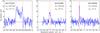Fig. 1 HI-line profiles for three representative ALFALFA sources. For each galaxy the velocity width, W50, is measured between the two outermost points where the flux density falls to 50% of the peak value (red vertical lines). Left panel: MW analog with a typical “double horned” profile, indicative of a mostly flat outer rotation curve. Central panel: dwarf galaxy with a “boxy” profile shape. Right panel: extreme dwarf galaxy with a clearly “single-peaked” profile, suggestive of a rising rotation curve. Keep in mind that narrow profiles can also correspond to intrinsically high-width objects that are oriented close to face-on. Note also that the velocity span of the x-axis in all three panels is the same (1800 km s-1), and so profile widths are plotted to scale.

Even though number counts of low-mass galaxies do not provide a stringent test of ΛCDM by themselves, they provide the basis for a different challenge that is much more difficult to resolve. Boylan-Kolchin et al. (2011) first identified the potential issue in the context of the MW satellites, and dubbed it the “too big to fail” (TBTF) problem. Given the low number of observed MW satellites, galaxy formation should be restricted to the few most massive subhalos of the MW. However, according to dark-matter-only (DM-only) simulations (Aquarius simulation; Springel et al. 2008), the likely hosts are too dense to be compatible with the measured kinematics of the MW satellites (Fig. 2 in Boylan-Kolchin et al. 2012).

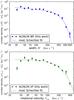Fig. 2 ALFALFA measurement of the width and rotational velocity functions. Top panel: data points represent the velocity width function (WF) of galaxies measured by ALFALFA, for galaxies with . The errorbars represent the 1σ counting noise (see Eq. (A.1)), and do not include any systematic uncertainties. The dotted line is a modified Schechter fit to the data (Eq. (1)), with parameters: $\log \mathrm{\left(}{\mathit{n}}_{\mathrm{\ast }}\mathrm{\right)}\mathrm{=}\mathrm{-}\mathrm{1.68}\mathrm{\pm }\mathrm{0.20}\hspace{0.17em}{\mathit{h}}_{\mathrm{70}}^{\mathrm{3}}{\mathrm{Mpc}}^{-3}\hspace{0.17em}{\mathrm{dex}}^{-1}$, log (W∗) = 2.52 ± 0.076 km s-1, α = −0.45 ± 0.24 and β = 2.39 ± 0.50. Bottom panel: data points represent the rotational velocity function (VF) of galaxies measured by ALFALFA, again for galaxies with . Rotational velocities, Vrot, have been obtained from inclination-corrected velocity widths according to Eq. (2). Errorbars again represent the 1σ counting noise, and do not include any systematic uncertainties. The dotted line is a modified Schechter fit to the data, with parameters: $\log \mathrm{\left(}{\mathit{n}}_{\mathrm{\ast }}\mathrm{\right)}\mathrm{=}\mathrm{-}\mathrm{1.17}\mathrm{\pm }\mathrm{0.25}{\mathit{h}}_{\mathrm{70}}^{\mathrm{3}}{\mathrm{Mpc}}^{-3}\hspace{0.17em}{\mathrm{dex}}^{-1}$, log (V∗) = 2.04 ± 0.18 km s-1, α = 0.14 ± 0.41 and β = 1.46 ± 0.37.

Despite its theoretical appeal, the TBTF problem as stated above has its own weak points as a test of ΛCDM. For example, it relies on observations of the satellites of just one galaxy, the MW. In addition, actual MW satellites are expected to be affected more by environmental effects than their DM-only counterparts. These considerations highlight the importance of assessing whether a similar issue is also present beyond the context of the MW. Recently, Tollerud et al. (2014) showed that the satellites of the Andromeda galaxy (M 31) also face a TBTF problem. Based on statistical arguments, Rodríguez-Puebla et al. (2013) further suggested that the TBTF problem should be generically present for MW-sized galaxies. Most importantly however, the work of Ferrero et al. (2012) showed that an analogous issue may be present for dwarf galaxies in the field¹. They argued that, based on the number density of galaxies measured by the Sloan Digital Sky Survey (e.g., Baldry et al. 2008; Li & White 2009), virtually all galaxies in a ΛCDM universe should be hosted by halos with M_vir ≳ 10¹⁰ M_⊙. However, the rotation curves of many low-mass dwarfs indicate that they are hosted by halos below this expected mass “threshold”. The result of Ferrero et al. (2012) is also supported by the very recent work of Kirby et al. (2014) and Garrison-Kimmel et al. (2014), who show that the TBTF problem is present for non-satellite galaxies in the Local Group, as well.

In this work, we perform a similar analysis to that of Ferrero et al. (2012), but we use a highly complementary observational dataset: the sample of galaxies detected by the Arecibo Legacy Fast ALFA (ALFALFA) survey in the emission line of atomic hydrogen (HI). This allows us to address a range of observational and theoretical uncertainties present in earlier works, which are all based on optically selected samples. For example, the current optical census of low-mass galaxies in the nearby universe is incomplete, because optical surveys are biased against low surface brightness objects. In addition, galaxies have so far been statistically connected to halos based on their measured stellar masses. However, recent observational evidence (Garrison-Kimmel et al. 2014) suggests that this approach may not be valid in the low-mass regime.

The present article is organized as follows: in Sect. 2² we describe the measurement of the galactic velocity function from the ALFALFA survey. Details regarding the measurement process can be found in Appendix A. In the same section we also describe the abundance matching (AM) procedure used for connecting galaxies to their host halos. In Sect. 3 we present a sample of galaxies with resolved HI kinematics drawn from the literature, and we describe how we use their measured rotation curves to test the derived AM relation. The main result of this work is presented in Sect. 3.3; readers with limited available time may choose to directly refer to this paragraph. Appendix B contains additional galactic data that are relevant for the result presented in Sect. 3.3. In Sect. 4 we elaborate on the importance of our findings in the context of small-scale tests of ΛCDM. In the same section we also point out the main uncertainties and assumptions that can have a significant impact on the results of this work. Lastly, we end with a brief summary in Sect. 5.

2. Connecting observed galaxies with their host DM halos

2.1. Measuring the velocity function of galaxies

We measure galaxy rotational velocities using data from the publicly available catalog of the ALFALFA survey, which covers about 40% of the final survey area (α.40 catalog; Haynes et al. 2011). Since ALFALFA is a spectroscopic survey, each α.40 source has a measured spectrum of its HI line emission. Figure 1 illustrates how velocity widths, W₅₀, are measured from each source’s lineprofile. The velocity width reflects the range of speeds at which atomic gas moves within the galactic potential (up to a projection on the line-of-sight), and therefore contains important information about the galactic kinematics.

The top panel of Fig. 2 shows the number density of galaxies as a function of their velocity width, as measured from the ALFALFA sample (blue datapoints). This distribution is referred to as the velocity width function (WF) of galaxies, and details on its calculation can be found in Appendix A. The measurement of the WF shown here refers to galaxies with HI masses of M_HI ≥ 10⁷ M_⊙ and velocity widths have been corrected for Doppler broadening as W = W₅₀/ (1 + z_⊙). We then perform an analytical fit to the WF (dotted blue line), of the modified Schechter functional form: $\begin{array}{ccc}\mathit{n}\mathrm{\left(}\mathit{W}\mathrm{\right)}\mathrm{=}\frac{\mathrm{d}{\mathit{n}}_{\mathrm{gal}}}{\mathrm{d}{\log }_{\mathrm{10}}\mathit{W}}\mathrm{=}\ln \mathrm{\left(}\mathrm{10}\mathrm{\right)}{\mathit{n}}_{\mathrm{\ast }}{\left(\frac{\mathit{W}}{{\mathit{W}}_{\mathrm{\ast }}}\right)}^{\mathit{\alpha }}{\mathrm{e}}^{\mathrm{-}{\left(\frac{\mathit{W}}{{\mathit{W}}_{\mathrm{\ast }}}\right)}^{\mathit{\beta }}}\mathit{.}& & \end{array}$(1)The best fit parameters are $\log \mathrm{\left(}{\mathit{n}}_{\mathrm{\ast }}\mathrm{\right)}\mathrm{=}\mathrm{-}\mathrm{1.68}\mathrm{\pm }\mathrm{0.20}{\mathit{h}}_{\mathrm{70}}^{\mathrm{3}}{\mathrm{Mpc}}^{-3}\hspace{0.17em}{\mathrm{dex}}^{-1}$, log (W_∗) = 2.52 ± 0.076 km s^-1, α = −0.45 ± 0.24 and β = 2.39 ± 0.50. We would like to stress that the quoted errors on the parameters do not include systematic uncertainties. We would also like to note that the fit parameters are strongly covariant, such that varying each of them independently within its 1σ range does not always produce an acceptable fit.

The WF has the distinct advantage of measuring the distribution of velocity width, W, which is a direct observable for an HI-line survey. At the same time however, W is measured in projection on the line-of-sight, and therefore does not correspond to any intrinsic galactic property. A more physically meaningful quantity can be derived from the inclination-corrected velocity width: if the inclination angle of a galaxy is i, we can define a measure of galactic rotational velocity as ${\mathit{V}}_{\mathrm{rot}\mathit{,}\mathrm{HI}}\mathrm{=}\mathit{W}\mathit{/}\mathrm{(}\mathrm{2}\mathrm{\times }\sin \mathit{i}\mathrm{)}\mathit{.}$(2)Given that all ALFALFA galaxies used in this work have assigned optical counterparts, we can indeed obtain estimates of V_rot for each object individually. In particular, we use the SDSS counterpart’s photometric axial ratio, b/a, to estimate galactic inclinations through the expression: 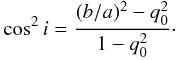$\begin{array}{ccc}{\cos }^{\mathrm{2}}\mathit{i}\mathrm{=}\frac{\mathrm{(}\mathit{b}\mathit{/}\mathit{a}{\mathrm{)}}^{\mathrm{2}}\mathrm{-}{\mathit{q}}_{\mathrm{0}}^{\mathrm{2}}}{\mathrm{1}\mathrm{-}{\mathit{q}}_{\mathrm{0}}^{\mathrm{2}}}\mathrm{·}& & \end{array}$(3)Here, q₀ = 0.13 is the assumed value of intrinsic axial ratio of galaxies viewed edge-on (Giovanelli et al. 1994). Then, the value of V_rot for each galaxy can be easily computed via Eq. (2), and the galactic number density as a function of V_rot can be measured according to Eq. (A.1). The resulting distribution is called the velocity function of galaxies (VF), and is shown in the bottom panel of Fig. 2. Low-inclination galaxies with sini< 2 / 3 were excluded from the measurement, in order to avoid making large inclination corrections. This restriction excludes about a quarter of the sample from the calculation (1657 out of 6770 galaxies), which we compensate for by uniformly increasing the normalization of the VF by the appropriate factor (6770 / 5113 ≈ 1.324). We also perform a modified Schechter fit to the measured VF (green dotted line). The best fit parameters are $\log \mathrm{\left(}{\mathit{n}}_{\mathrm{\ast }}\mathrm{\right)}\mathrm{=}\mathrm{-}\mathrm{1.17}\mathrm{\pm }\mathrm{0.25}{\mathit{h}}_{\mathrm{70}}^{\mathrm{3}}{\mathrm{Mpc}}^{-3}\hspace{0.17em}{\mathrm{dex}}^{-1}$, log (V_∗) = 2.04 ± 0.18 km s^-1, α = 0.14 ± 0.41 and β = 1.46 ± 0.37. We would like to stress again that the plotted errors on the VF datapoints do not include systematic uncertainties, and therefore neither do the quoted errors on the fit parameters. Note also that we exclude from the fit the lowest velocity bin, whose very low value may be an effect of measurement incompleteness.

2.2. Velocity abundance matching

Both the galactic VF and WF have been extensively used in the literature to test ΛCDM on galactic scales (Obreschkow et al. 2009, 2013; Zavala et al. 2009; Zwaan et al. 2010; Papastergis et al. 2011; Trujillo-Gomez et al. 2011; Schneider et al. 2014; Klypin et al. 2014). In particular, ΛCDM makes a concrete prediction for the halo velocity function (HVF), i.e., the number density of halos as a function of their maximum rotational velocity, V_h. As long as a theoretical model exists to compute the HI rotational velocity (or velocity width) of a galaxy inhabiting a given DM halo, one can make a prediction for the galactic VF that ought to be observed. In fact, semi-analytic and semi-empirical models have been relatively successful in reproducing the observed galactic VF at intermediate and high velocities, within the context of ΛCDM cosmology (Obreschkow et al. 2009, 2013; Trujillo-Gomez et al. 2011). However, theoretical predictions consistently overestimate the observed number density of dwarf galaxies with V_rot≲60−80 km s^-1 (Zavala et al. 2009; Trujillo-Gomez et al. 2011; Schneider et al. 2014). This is true even for more refined models based on hydrodynamic simulations, which have trouble reproducing observations at low velocities as well (see, e.g., Sawala et al. 2013, Fig. 10). At the same time, it is important to keep in mind that the models mentioned above implicitly assume that observed values of V_rot are effectively measuring the maximum rotational velocity of the host halos.

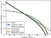Fig. 3 Cumulative velocity functions for galaxies and ΛCDM halos. The dashed black line represents the cumulative number density of halos as a function of their maximum circular velocity, Vh, in a ΛCDM universe (BolshoiP simulation; Hess et al., in prep.). The solid black line corresponds to the “galactic” HVF, which excludes massive halos that are unlikely to host individual galaxies (see Eq. (5)). The dotted green line shows the cumulative VF of ALFALFA galaxies. The red shaded region represents the VF of early-type galaxies, measured from SDSS data (Bernardi et al. 2010). The solid green line represents the VF of galaxies of all morphological types, obtained from the sum of the ALFALFA and early-type VFs.

In view of the difficulties faced by theoretical models in reproducing the observed VF of galaxies, we take here a more conservative approach: we use the galactic VF measured by ALFALFA to infer the expected relation between V_rot and V_h in a ΛCDM universe. Our approach therefore does away with the assumption that V_rot is approximately equal to V_h.

We then go ahead and infer a quantitative V_rot − V_h relation by using the statistical technique of abundance matching (AM). AM operates under the assumption that galaxies with higher V_rot are hosted on average by halos with higher V_h (see discussion in Sect. 4.3). Thus V_h(V_rot) can be derived by matching the cumulative number densities of galaxies and halos, i.e., by demanding that 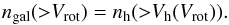${\mathit{n}}_{\mathrm{gal}}\mathrm{(}\mathit{>}{\mathit{V}}_{\mathrm{rot}}\mathrm{)}\mathrm{=}{\mathit{n}}_{\mathrm{h}}\mathrm{(}\mathit{>}{\mathit{V}}_{\mathrm{h}}\mathrm{(}{\mathit{V}}_{\mathrm{rot}}\mathrm{\left)}\mathrm{\right)}\mathit{.}$(4)The number density of halos on the right hand side of the equation above also includes the contribution of subhalos.

Figure 3 shows the cumulative velocity distributions of galaxies and halos used in the AM procedure. Specifically, we use the halo velocity function, n_h( >V_h), of the BolshoiP ΛCDM simulation (Hess et al., in prep.). The BolshoiP simulation assumes a Planck first-year cosmology (Planck Collaboration XVI 2014), and therefore predicts a higher normalization for the halo velocity function (HVF) than its WMAP7 predecessor (Bolshoi simulation; Klypin et al. 2011). The cumulative VF of ALFALFA galaxies is also shown in Fig. 3. It is calculated by integrating the fit to the differential galaxy VF (see bottom panel of Fig. 2). It is important to notice that the HVF in a ΛCDM universe is significantly steeper than the observed galactic VF, which is the reason why theoretical models generically overpredict the number of low-velocity galaxies.

Before we can proceed, we need to address here two complications: firstly, massive halos with M_vir ≳ 2 × 10¹³ M_⊙ are usually not the hosts of individual galaxies, but rather of galactic groups or clusters. We therefore use the factor ${\mathit{f}}_{\mathrm{g}}\mathrm{\left(}{\mathit{V}}_{\mathrm{h}}\mathrm{\right)}\mathrm{=}{\mathrm{e}}^{\mathrm{-}\mathrm{(}{\mathit{V}}_{\mathrm{h}}\mathit{/}\mathrm{330}\mathrm{km}{\mathrm{s}}^{-1}{\mathrm{)}}^{\mathrm{3}}}$(5)to suppress the high-velocity end of the HVF, n_g(V_h) = f_g(V_h) × n(V_h). The resulting “galactic” HVF approximately matches the results of Shankar et al. (2006) and Rodríguez-Puebla et al. (2011).

The second complication stems from the fact that blindly selected HI samples have a bias against gas-poor, early-type galaxies. This can be seen directly by placing ALFALFA detections on a color-magnitude diagram (Huang et al. 2012, Fig. 10), but also indirectly by measuring the clustering properties of ALFALFA galaxies (Papastergis et al. 2013, Fig. 13). To compensate for this effect we consider the work of Bernardi et al. (2010), who have used SDSS spectra to measure stellar velocity dispersions for galaxies of different morphological types. Their results for the cumulative VF for early-type galaxies is shown in Fig. 3. We use two empirical relations to transform the SDSS-based velocity dispersions into equivalent rotational velocities: Eq. (3) in Baes et al. (2003) and Eq. (2) in Ferrarese (2002; with the parameters appropriate for elliptical galaxies as given in their Table 2). The plotted range of the early-type VF reflects the difference between the two relations, and illustrates the typical (small) uncertainty associated with such transformations.

Lastly, we obtain the VF for all galaxies (regardless of type) from the sum of the ALFALFA VF and the VF of early-type objects measured by Bernardi et al. Keep in mind that the measurement of Bernardi et al. is restricted to velocities ≳100 km s^-1; Therefore, we implicitly assume that the HI-selected ALFALFA sample is a complete census of low-velocity galaxies (but see Sect. 4.2 for a discussion).

Fig. 4 Vrot − Vh relation in a ΛCDM universe. The blue line is the average relation between the galactic HI rotational velocity (Vrot) and the maximum circular velocity of the host halo (Vh), in a ΛCDM universe. This relation is obtained by abundance matching (AM), i.e., by matching the cumulative velocity distributions of all galaxies and “galactic” halos (see Fig. 3). The dashed blue line is the AM result when galaxies are matched to all halos. The dashed black line is a reference one-to-one line.

In Fig. 4 we present the average V_rot − V_h relation expected in a ΛCDM universe, derived through AM. Specifically, the relation is obtained by matching the cumulative number densities of “galactic” halos and galaxies of all types (see Fig. 3). V_rot is greater than V_h at intermediate and high velocities, reaching maximum ratios of V_rot/V_h ≈ 1.4. Ratios larger than unity can be achieved when there is a large baryonic contribution to the galactic rotation curve (RC), which leads to a substantial boost to the rotational velocity (see e.g., Trujillo-Gomez et al. 2011, Fig. 5). Keep in mind however, that the exact behavior of the AM relation at velocities V_rot≳ 250 km s^-1 is relatively uncertain. For example, Fig. 4 also shows the AM result when all halos are included. Moreover, the addition of a modest amount of scatter to the idealized Eq. (4) will have a similar effect, namely it will alter the high-velocity end of the relation.

Most importantly however, the relation displays a remarkable “downturn” at low velocities, whereby the V_rot of dwarf galaxies is predicted to significantly underestimate the V_h of their hosts. This effect is expected to become more pronounced as the measured HI velocity decreases: for example, galaxies with V_rot = 15−20 km s^-1 are expected to reside in halos with V_h≈ 40–45 km s^-1. This behavior has a simple and intuitive explanation: if halos with V_h< 40 km s^-1 were allowed to host galaxies that are detectable by ALFALFA, then the galactic number density in a ΛCDM universe would be much larger than observed (refer to Fig. 3). The discussion above does not change even in the presence of scatter in the V_rot − V_h relation, because scatter does not affect the AM result at the low end³.

3. Internal kinematics of dwarf galaxies

3.1. Data sample

In this section we aim to place individual galaxies on the V_rot − V_h diagram shown in Fig. 4, in order to observationally test the relation predicted by ΛCDM. Ideally, one would like to place on the diagram the same objects that went into calculating the galactic VF; this would ensure that the AM relation is derived using the same objects that are used for testing it. Unfortunately however, the data provided by ALFALFA are not sufficient to accomplish this task. In particular, even though ALFALFA data can be used to derive values of V_rot (in conjunction with optical inclinations), they do not contain enough information to constrain V_h.

We therefore use instead an extensive sample of galaxies with interferometric HI observations, gathered from the literature. In particular, we use 12 galaxies from Sanders (1996), 30 galaxies from Verheijen & Sancisi (2001), 19 galaxies from The HI Nearby Galaxy Survey (THINGS; de Blok et al. 2008; Oh et al. 2011a), 54 galaxies from the Westerbork HI Survey of Spiral and Irregular Galaxies (WHISP; Swaters et al. 2009, 2011), 12 galaxies from the Local Volume HI Survey (LVHIS; Kirby et al. 2012), 5 galaxies from Trachternach et al. (2009), 4 galaxies from Côté et al. (2000), 28 galaxies from the Faint Irregular Galaxies GMRT Survey (FIGGS; Begum et al. 2008a,b), 17 galaxies from the LITTLE THINGS survey (Hunter et al. 2012; Oh et al., in prep.), 11 galaxies from the SHIELD survey (Cannon et al. 2011), and the recently discovered galaxy Leo P (Bernstein-Cooper et al. 2014).

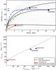Fig. 5 Kinematic analysis of galaxies with HI rotation curves. Top panel: three representative rotation curves (RCs) from the literature sample of galaxies with interferometric HI observations (red: UGC 7577, green: UGC 7323; blue: UGC 8490). The gray solid lines show the RCs of increasingly more massive NFW halos (from bottom to top). The concentration parameter for each halo is the median concentration expected for its mass in a Planck cosmology (Dutton & Macciò 2014). The three thick gray lines show the most massive NFW halos that are compatible with the last measured point of each galaxy’s RC (large colored symbols), to within 1σ. For each galaxy, only the last measured point of the RC is used for the analysis in this work. The peak velocity for each of these three halos is the value of Vh assigned to the corresponding galaxy. The colored horizontal marks denote the value of Vrot for the three galaxies, inferred from their inclination-corrected linewidths (see Eq. (2)). Bottom panel: small circles show the placement of UGC 7577, UGC 7323 and UGC 8490 on the Vrot − Vh diagram, according to the procedure outlined in the top panel. The large diamonds show their positions after a correction is applied to account for the cosmic baryon fraction (see text for details).

The sample of individual objects assembled above is inhomogeneous, but spans an impressive range of observed rotational velocities: from >300 km s^-1 for galaxy UGC2885 in the Sanders (1996) sample to ≈12 km s^-1 for galaxy KK44 in the FIGGS sample. This means that the kinematics of galaxies of very different sizes are modeled to different levels of detail. For example, most of the spiral galaxies in the THINGS sample analyzed by de Blok et al. (2008) have RCs of exquisite resolution, and mass models constrained by multiwavelength data. On the other hand, the velocity fields of the extremely low-mass SHIELD galaxies are significantly harder to model, and only outermost-measured-point velocity estimates are available for them at present. We would like to note that the objects in the literature sample do not share the same selection rules as the α.40 sample; for example, some of the galaxies with interferometric observations have D< 7 Mpc or M_HI< 10⁷ M_⊙. Keep also in mind that all galaxies have been observed as part of targeted HI interferometric campaigns. As a result, almost all galaxies are relatively gas-rich and fairly isolated; this means that the vast majority of the objects are field galaxies.

3.2. Kinematic analysis

Figure 5 illustrates the process used to place galaxies on the V_rot − V_h diagram. We use three galaxies as examples, taken from the Swaters et al. (2011) sample: UGC 7577, UGC 7323 and UGC 8490. Their RCs are shown in the top panel of Fig. 5. For each galaxy, the last measured point (LMP) of its RC is marked with a bold symbol; this is the only datapoint used in this work to constrain V_h.

We then consider a set of DM halos with monotonically increasing masses. The DM halos are assumed to have an NFW mass profile (Navarro et al. 1997) of the form $\mathit{\rho }\mathrm{\left(}\mathit{R}\mathrm{\right)}\mathrm{=}\frac{{\mathit{\rho }}_{\mathrm{0}}}{\frac{\mathit{R}}{{\mathit{R}}_{\mathrm{s}}}\left[\mathrm{1}\mathrm{+}{\mathrm{(}{\frac{\mathit{R}}{{\mathit{R}}_{\mathrm{s}}}}^{\mathrm{)}}}^{\mathrm{2}}\right]}\mathrm{·}$(6)R_s and ρ₀ are the scale radius and scale density, respectively. In practice, halos are more often described in terms of virial quantities: in this work we define the virial radius, R_vir, at a density contrast of 104 with respect to the critical density⁴ (R_vir = R_104c). Then we can define the virial velocity as the circular velocity of the halo at the virial radius, V_vir = V(R_vir), and the concentration parameter as c = R_vir/R_s. Therefore V_vir and c describe “how massive” and “how dense” a halo is, respectively. The RC of an NFW halo can now be written as ${\mathit{V}}_{\mathit{c}}\mathrm{\left(}\mathit{R}\mathrm{\right)}\mathrm{=}{\mathit{V}}_{\mathrm{vir}}\mathrm{\times }\sqrt{\frac{\ln \mathrm{(}\mathrm{1}\mathrm{+}\mathit{cx}\mathrm{)}\mathrm{-}\frac{\mathit{cx}}{\mathrm{1}\mathrm{+}\mathit{cx}}}{\mathit{x}\mathrm{(}\ln \mathit{c}\mathrm{-}{\frac{\mathit{c}}{\mathrm{1}\mathrm{+}\mathit{c}}}^{\mathrm{)}}}}\mathit{,}$(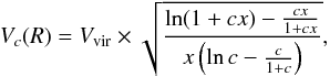7)where x = R/R_vir is the normalized radius.

We identify the most massive halo that is compatible with the velocity measured at the LMP for each of the three example galaxies, to within the 1σ velocity error. The peak RC amplitude for each of these three halos is the value of V_h assigned to the corresponding galaxy. It is important to keep in mind that for most objects the maximum halo velocity is reached beyond the extent of the galaxy’s RC. For example, the RC of UGC 7323 extends to R = 5.9 kpc, but its host halo achieves its maximum velocity of 117.1 km s^-1 at R = 32.9 kpc. The procedure above does not assume a priori that V_rot≈V_h, as is usual practice in many theoretical works. In fact, galaxies with less extended RCs (e.g., UGC 7323), can be assigned V_h values that are significantly higher than their V_rot.

The values of V_rot for each example galaxy are computed based on the observed width of the galactic lineprofile, W, and the galaxy inclination, i (Eq. (2)). The profile widths of galaxies in our literature sample can be obtained from either their interferometric or previous single-dish observations. Their inclinations, i, can be derived in a variety of ways, depending on the data quality: When the galactic velocity field is well resolved, the inclination can be measured by modeling the observed kinematics. When this is not possible, one can use the axial ratio of the spatially resolved HI emission to infer the inclination of the gaseous disk. If neither method is practical, the photometric axial ratio of the optical counterpart can be used instead (as per Eq. (3)). In general, kinematic inclinations and inclinations based on the HI axial ratio are thought to be more accurate than optical ones (Kirby et al. 2012; Verheijen & Sancisi 2001).

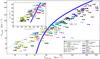Fig. 6 Placement of galaxies on the Vrot − Vh diagram. Main figure: the blue line is the average Vrot − Vh relation in a ΛCDM universe, inferred from abundance matching (same as in Fig. 4). The colored points represent a sample of 194 galaxies with interferometric HI observations, drawn from the literature. Their Vrot and Vh values are computed as described in Fig. 5. All points are drawn as upper limits, because we make the conservative assumption that the contribution of baryons to the galactic RC is negligible for all galaxies. Refer to Sects. 3.3 and 4 for the scientific interpretation of this figure. Inset panel: a zoom-in on the low-velocity region of the diagram (linear axes).

The bottom panel of Fig. 5 shows the positions of the three example galaxies on the V_rot − V_h diagram, based on the analysis described above. Note that for a fixed value of V_rot, galaxies with a more extended RC can place a more stringent constraint on V_h. This is immediately obvious by comparing the position of galaxies UGC 8490 and UGC 7323 on the V_rot − V_h diagram, and noting the extent of their RCs in the top panel of Fig. 5.

Let us now point out two complications related to the procedure described above: first, the AM result refers to V_h values for the halos in the BolshoiP simulation, where the total matter content of the universe (Ω_m = Ω_DM + Ω_bar) is treated as a dissipationless fluid. This means that, if f_bar ≈ 0.15 is the cosmic baryon fraction, a realistic halo would have a factor of (1 − f_bar) less DM mass than its corresponding BolshoiP halo. The rest of the mass would be in the form of baryons, part of which will end up in the galactic disk in the form of stars or gas. Ideally, one would subtract the contribution of baryonic components from a galaxy’s RC before using it to constrain the host halo mass. However, here we do not attempt to calculate baryon-subtracted RCs; we make instead the conservative assumption that the RCs of all galaxies in our sample are fully attributable to DM. Therefore, we simply increase the derived value of V_h by a factor of (1 − f_bar)^{− 1 / 3}, in order to reflect the higher DM content of the simulation (the 1 / 3 exponent follows from the ${\mathit{M}}_{\mathrm{vir}}\mathrm{\propto }{\mathit{V}}_{\mathrm{h}}^{\mathrm{3}}$ scaling for DM halos). These new V_h estimates are overly conservative in the case of large spiral galaxies, whose RCs have a sizable contribution from baryons. However, the rescaled V_h values are fairly realistic for dwarf galaxies, which are typically DM-dominated (e.g., Papastergis et al. 2012; Sawala et al. 2013).

Second, as one can realize from inspection of Eq. (7), it is not possible to determine a unique value for V_h given only one point of the galactic RC. The reason is that the RCs of NFW halos are a two-parameter family: one can find a wide range of compatible halos, by simply adjusting the values of V_vir and c. In this work, we fix c to the median value as a function of halo mass, as expected in a Planck cosmology (Table 3 in Dutton & Macciò 2014).

In principle, one could use the whole RC of a galaxy to simultaneously fit for V_h and c. In fact, such an analysis is available for several galaxies in our sample (de Blok et al. 2008; Oh et al. 2011a; Swaters et al. 2011). However, as shown by the RC of UGC 7577, these studies find that NFW halos of median concentration do not provide a good description of the inner velocity profiles of dwarf galaxies (e.g., Oh et al. 2011a). Recently, hydrodynamic simulations have shown that the inner DM profiles of halos can be affected by baryonic feedback processes (e.g., Governato et al. 2010), resulting in RCs that better match the observations of the inner velocity profiles of dwarfs (Oh et al. 2011b). Consequently, one may repeat the kinematic analysis described in this section using instead a velocity profile that captures the modification of the galactic RC induced by feedback (e.g., Di Cintio et al. 2014a,b). In such case, the value of V_h assigned to a given galaxy can, in principle, be substantially different from the value obtained from an NFW analysis (Brook & Di Cintio 2014). This fact represents an important caveat in the kinematic analysis described in this section, which we would like to fully acknowledge. At the same time, the NFW analysis can still produce reliable results, provided that the difference between the modified profile and its unmodified NFW counterpart is small at the radius of the galaxy’s LMP (see Appendix B). We devote Sect. 4.4 to assess to what extent the effect of feedback on the velocity profiles of halos can affect the results of this article.

3.3. Results

Figure 6 shows the placement on the V_rot − V_h diagram of all the 194 galaxies with literature HI rotation curves. Twelve galaxies have duplicate entries in more than one of the samples listed in Sect. 3.1, in which cases we plot the observation corresponding to the most extended RC (taking data quality into consideration as well). All galaxies are positioned as upper limits on the diagram, because their V_h values refer to the most massive compatible halo.

Over most of the range in HI rotational velocity, 30 km s^-1≲V_rot≲ 300 km s^-1, the AM relation is consistent with the upper limits obtained from individual galaxies. Most importantly though, the situation changes at the lowest velocities probed: for example, when one considers galaxies with V_rot< 25 km s^-1, all but three of the upper limits are inconsistent with the AM relation. We have verified that this result holds even if we substitute median concentration halos in our kinematic analysis with 2σ under-concentrated ones. The inconsistency arises because the AM relation predicts fairly massive hosts for the lowest-velocity galaxies in our sample; however, such massive halos would exceed the velocity measured at the LMP for these objects. A different way of phrasing the inconsistency is that, if halos with V_h≲ 30 km s^-1 were allowed to host the lowest-velocity galaxies in our sample (as the galactic kinematics indicate), then their number density in a ΛCDM universe would be much higher than what observed by ALFALFA. Figure B.1 offers yet another way to visualize the inconsistency in an intuitive fashion.

Before we proceed with a discussion of the scientific relevance of this result, we would like to point out a number of subtleties related to the positioning of objects on the V_rot − V_h diagram.

First, the RCs of DM halos described by Eq. (7) represent the halo circular velocity at each radius, which reflects the enclosed dynamical mass. However, the gas in actual galaxies undergoes some turbulent motion in addition to rotation, with typical amplitudes of 8–10 km s^-1. As a result, observed RCs should be corrected for pressure support before being compared to theoretical halo RCs. These corrections are most important for the lowest velocity galaxies in our sample, where ordered rotation and turbulent motion have similar amplitudes. Pressure support corrections have been performed in the original sources for the galaxies in the THINGS, LITTLE THINGS, FIGGS and Côté et al. (2000) samples, as well as for LeoP. On the other hand, no corrections have been originally applied to the galaxies in the WHISP and SHIELD samples. For galaxies in these two samples we apply a crude pressure support correction to their LMP, 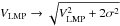${\mathit{V}}_{\mathrm{LMP}}\mathrm{\to }\sqrt{{\mathit{V}}_{\mathrm{LMP}}^{\mathrm{2}}\mathrm{+}\mathrm{2}{\mathit{\sigma }}^{\mathrm{2}}}$, assuming σ = 8 km s^-1. The correction increases the LMP velocity somewhat, and therefore results in a slightly higher value of V_h.

Second, galactic RCs have been checked for their quality, to the extent allowed by the material published in each original reference. In cases where the velocity for the originally published outermost radius was deemed unreliable, we adopted a measurement at a smaller radius as our LMP. Even though this process is highly subjective, any truncation of the original RC is conservative for the purposes of this work (see Sect. 3.2). Note also that for the extreme dwarf galaxies of the FIGGS, LITTLE THINGS and SHIELD samples no quality control was performed, since the only available data were LMP radii and velocities.

Third, we have given no information regarding the observational errors associated with the placement of each galaxy on the V_rot − V_h diagram. Unfortunately, we cannot quantify the errors on both V_rot and V_h for each galaxy in a rigorous way, but we would like to offer some qualitative guidance. The error on V_rot is determined by the measurement error on the velocity width and the uncertainty on the adopted inclination value. These errors are not always quoted in the original references. Typical values for the former are a few km s^-1, while values for the latter depend on the method used to determine the inclination (≈5° for kinematic inclinations of good quality, larger in other cases). In the case of low inclination galaxies, a small error in inclination can translate into a fairly large error on V_rot. Keep also in mind that it is difficult to quantify the systematic component of the inclination uncertainty, especially when different methods are used for different objects.

Errors on V_h are even harder to quantify: they depend on the error with which the LMP velocity and radius are measured. The LMP velocity error mainly depends on the inclination uncertainty (discussed above). However, keep in mind that if the velocity field is asymmetric, or if there are significant non-circular motions, systematic uncertainties arise that are difficult to quantify. The LMP radius, on the other hand, is affected by distance uncertainties; this is because the conversion from an angular extent on the sky to physical units (kpc) is distance-dependent. The uncertainty on the distance varies a lot form object to object: some galaxies in our sample have accurate primary distances (e.g., TRGB), while others have lower accuracy distances based on flow models or even pure Hubble flow.

In general, errors on inclination affect both V_rot and V_h. As a result, galaxies move roughly diagonally on the V_rot − V_h diagram. On the other hand, errors on the distance only affect V_h. This causes galaxies to move horizontally on the diagram.

4. Discussion

The TBTF issue was first identified in the MW system, as an incompatibility between the measured kinematics of the brightest MW satellites and the kinematics of their expected host subhalos in ΛCDM simulations (Boylan-Kolchin et al. 2011). However, a number of possible solutions to the MW TBTF problem within the ΛCDM model have been identified, thus disputing the cosmological significance of the discrepancy. For example, Wang et al. (2012) and Vera-Ciro et al. (2013) have argued that if the mass of the MW halo is M_vir< 1 × 10¹² M_⊙ then the TBTF problem would likely not occur. This is because the typical masses of the largest subhalos scale sensitively with the mass of the host halo. A MW mass in this range is on the low side of observational estimates (e.g., Watkins et al. 2010), and is lower than typically assumed in DM simulations of MW analogs. Another solution can come from considering the cosmic variance associated with observations of a single object. Purcell & Zentner (2012) have argued that the TBTF problem is expected to occur in at least 10% of MW-sized halos just due to halo-to-halo variation in the subhalo population.

The plausibility of the two solutions above has since been put into question, because the TBTF problem is likely present in the satellite populations of galaxies other than the MW. For example, Tollerud et al. (2014) finds that the TBTF problem is also present in the satellite system of the Andromeda galaxy (M 31). This finding weakens the “light” MW argument, because it is unlikely that both the MW and Andromeda are hosted by halos with M_vir< 1 × 10¹² M_⊙ (van der Marel et al. 2012). It also weakens the cosmic variance argument, because it is improbable that both the MW and M31 are outliers in terms of their subhalo populations. In addition, Rodríguez-Puebla et al. (2013) find based on statistical considerations that the MW satellites are a fairly typical population for a galaxy of this size (see also Strigari & Wechsler 2012).

Nonetheless, a different potential solution to the TBTF has been put forward by Zolotov et al. (2012), which is generically applicable to the satellite population of any MW-sized halo. This solution is related to baryonic effects that had not been taken into account in the original TBTF formulation. In particular, Zolotov et al. argue that internal feedback processes in low-mass halos (e.g., gas blowout due to star formation) will lead to the formation of low-density “cores” in their inner DM profiles. This fact, in conjunction with the presence of a stellar disk in the MW, will lead to significantly enhanced tidal stripping of subhalos compared to the DM-only case. As a result, a significant amount of mass can be removed from the central parts of subhalos, leading to velocity profiles that are consistent with measurements (see Fig. 3 in Brooks & Zolotov 2014). This baryonic solution to the TBTF problem has been regarded as a generic and robust way to resolve the discrepancy. However, the proposed mechanism relies on processes that are specific to satellite galaxies; this is why establishing whether the TBTF problem is also present for field galaxies has important scientific implications.

The first evidence for a positive answer came from the work of Ferrero et al. (2012). In particular, they used the stellar mass function (SMF) of galaxies to infer an M_∗ − M_h relation in a ΛCDM universe, via the technique of abundance matching. They then showed that the rotation curves of gas-rich galaxies with low stellar masses (M_∗ ≲ 10⁷ M_⊙) cannot accommodate host halos as massive as expected in ΛCDM (see their Fig. 3). The present work confirms the results of Ferrero et al., and at the same time addresses a number of systematic uncertainties present in their analysis. First, the SMF measured by current wide-area optical surveys, such as the SDSS, suffers from surface brightness incompleteness at low stellar masses (M_∗ ≲ 3 × 10⁸ M_⊙; see Fig. 6 in Baldry et al. 2008). As a result, the low-mass end of the SMF could be much steeper than the measured one, in which case the discrepancy reported by Ferrero et al. could be significantly alleviated or perhaps resolved (see Ferrero et al. 2012, Fig. 4). In the contrary, the measurement of the galactic VF from the ALFALFA HI-selected sample does not share the same surface brightness incompleteness; in fact, low surface brightness galaxies in the field are expected to be gas-rich, and therefore easily detectable by ALFALFA. Barring therefore the presence of a dominant population of low surface brightness and gas-poor galaxies in the field, the present estimates for the number density of low-mass galaxies seem robust (see also Sect. 4.2).

In addition, the AM procedure in Ferrero et al. is performed on the basis of stellar mass, as is the case in all previous works assessing the TBTF problem (Boylan-Kolchin et al. 2011; Tollerud et al. 2014; Garrison-Kimmel et al. 2014). This implicitly assumes that there is a monotonic relation between M_∗ and M_h (or V_h). However, Garrison-Kimmel et al. (2014) have used the stellar kinematics of local group galaxies to investigate whether such a relation is indeed present at very low masses; under the assumption of a universal halo mass profile, they find that for galaxies with M_∗ ≲ 10⁸ M_⊙ the stellar mass shows very little correlation with the inferred V_h,max (see their Fig. 12). By contrast, Fig. 6 seems to justify the velocity-based AM procedure used in this work. In particular, the datapoints show a clear monotonic trend between V_rot and V_h, down to the lowest velocities probed. In addition, V_rot values at fixed V_h show a well-behaved and relatively small scatter⁵ of 0.1 dex.

Lastly, most of the extremely low-velocity HI rotation curves analyzed by Ferrero et al. belong to galaxies in the FIGGS sample. This means that their results regarding the low-velocity end are susceptible to systematics or selection effects that are specific to this one sample. In this work we have significantly increased the number of extreme dwarf galaxies, by adding objects from the SHIELD and LITTLE THINGS projects. Reassuringly, Fig. 6 shows no discernible differences among the various dwarf samples.

Apart from the observational factors mentioned in Sect. 3.3, a number of other uncertainties and assumptions may affect the analysis performed this work. In the remainder of this section we consider in detail several such issues, and we show that they do not have a large impact on our main conclusions (at least when considered individually).

4.1. Measurement uncertainties on the galactic VF?

An accurate determination of the galactic VF is of great importance in the context of Fig. 6: in particular, the measured number density of galaxies with low velocities determines the exact behavior of the V_rot − V_h AM relation at the low-velocity end.

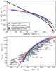Fig. 7 Observational uncertainties on the VF measurement. Top panel: the blue shaded region shows the range of ALFALFA cumulative VFs that correspond to modified Schechter parameters within 1σ from the best fit values (see Eq. (1)). The cyan line corresponds to the result of the HIPASS 21 cm survey (Zwaan et al. 2010), while the red line represents the cumulative VF measured in the Local Volume by Klypin et al. (2014). The two latter results are plotted to illustrate the magnitude of systematic uncertainties affecting the measurement of the VF. Bottom panel: the gray symbols represent our sample of galaxies with literature HI rotation curves (same as in Fig. 6). The colored lines represent the Vrot − Vh relation that corresponds to each of the cumulative VFs plotted in the upper panel, using the same color coding.

In Fig. 7 we illustrate how uncertainties on the measurement of the VF can impact the analysis in this article: The blue shaded region in the top panel of the figure shows the statistical uncertainty in the measurement of the ALFALFA VF. More specifically, the plotted range in the cumulative VF is derived from the 1σ parameter range of the modified Schechter fit to the differential ALFALFA VF (see Fig. 2).

We also plot in the same panel two recent literature determinations of the galactic VF, in order to illustrate the systematics affecting the measurement. First, we show the result obtained by the HI Parkes All Sky Survey (HIPASS), which is a blind, wide-area 21 cm survey that predated ALFALFA (Zwaan et al. 2010). Second, we show the distribution measured within the Local Volume by Klypin et al. (2014). The measurement is based on a nearly volume-complete catalog of galaxies within D< 10 Mpc (Karachentsev et al. 2013), and so it also includes gas-poor systems that may be missing from an HI-selected sample.

The bottom panel of Fig. 7 shows the resulting V_rot − V_h relations obtained from each of the cumulative VFs plotted in the upper panel. As we can clearly see by comparing the results of ALFALFA and HIPASS, a difference in the normalization of the VF leads to a shift in the inferred V_rot − V_h relation. Moreover, differences in the measured low-velocity slope of the VF affect the sharpness of the relation’s “downturn”. This is evident by comparing the ALFALFA and Local Volume results. Overall, however, the bottom panel demonstrates that random and systematic observational uncertainties on the inferred V_rot − V_h relation do not seem to strongly affect the conclusions reached in Sect. 3.3.

4.2. Low-velocity gas-poor galaxies?

The ALFALFA VF is not a complete census of galaxies in the universe, since objects with M_HI< 10⁷ M_⊙ are not included in the measurement. As shown in Sect. 2.2, HI selection can complicate the measurement of the VF at the high-velocity end, where massive early-type galaxies dominate (see also extensive discussion in Obreschkow et al. 2013). Similarly, we expect that HI selection will exclude a portion of the galactic population at low velocities, as well. Some of the excluded objects will be gas-poor early-type dwarfs, which are usually found in dense environments or as satellites of larger hosts (e.g., Geha et al. 2012). This population is not expected to be large, since the vast majority of dwarf galaxies correspond to star-forming systems with late-type morphologies (e.g., Karachentsev et al. 2013, Fig. 11; Baldry et al. 2012, Fig. 15). At the same time however, some fraction of late-type objects will also be excluded, simply because galaxies with low V_rot tend to have low gas masses.

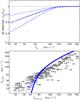Fig. 8 Incompleteness of the ALFALFA survey at low velocities. Top panel: the blue dotted, dashed and dash-dotted lines represent three relations for the “HI-selection” factor, fHI(Vrot), each accounting for progressively more low-velocity systems that are undetectable by ALFALFA due to their low HI mass (Eqs. (9)–(11)). Bottom panel: the blue dotted, dashed and dash-dotted lines are the average Vrot − Vh relations for the corresponding fHI(Vrot) relations shown in the top panel. For reference, we also plot our fiducial relation with a thick solid blue line (same as in Fig. 4). The gray symbols represent our sample of galaxies with HI rotation curves, same as in Fig. 6.

In order to explore this effect, we introduce here an “HI-selection” factor, f_HI(V_rot): it represents the fraction of galaxies at a given rotational velocity that are accounted for in the ALFALFA VF. We parametrize f_HI(V_rot) with the following analytical form: ${\mathit{f}}_{\mathrm{HI}}\mathrm{\left(}{\mathit{V}}_{\mathrm{rot}}\mathrm{\right)}\mathrm{=}{\mathit{f}}_{\mathrm{HI}\mathit{,}\mathrm{0}}\mathrm{\times }{\mathrm{2}}^{\mathrm{-}\frac{\mathit{\alpha }}{\mathit{\gamma }}}\mathrm{\times }{\left(\frac{{\mathit{V}}_{\mathrm{rot}}}{\begin{array}{c}\mathrm{˜}\\ \mathit{V}\end{array}}\right)}^{\mathit{\alpha }}\mathrm{\times }{\left[\frac{\mathrm{1}}{\mathrm{2}}\mathrm{+}\frac{\mathrm{1}}{\mathrm{2}}{\left(\frac{{\mathit{V}}_{\mathrm{rot}}}{\begin{array}{c}\mathrm{˜}\\ \mathit{V}\end{array}}\right)}^{\mathit{\gamma }}\right]}^{\mathrm{-}\frac{\mathit{\alpha }}{\mathit{\gamma }}}\mathrm{·}$(8)The equation above describes a power-law with exponent α at low velocities, that transitions to a constant value of f_HI,0 at high velocities. The parameter $\begin{array}{c}{\mathrm{˜}}_{}\\ \mathit{V}\end{array}$ determines the location of the transition, while γ controls its sharpness.

Since it is hard to observationally constrain f_HI(V_rot), we consider three cases that correspond to progressively larger populations of gas-poor galaxies at low velocities. They correspond to the following set of $\mathrm{\left[}{\mathit{f}}_{\mathrm{HI}\mathit{,}\mathrm{0}}\mathit{,}\begin{array}{c}{}_{\mathrm{˜}}\\ \mathit{V}\end{array}\mathit{,\alpha ,\gamma }\mathrm{\right]}$ parameters: $\begin{array}{ccc}{\mathit{f}}_{\mathrm{HI}}^{\mathrm{\left(}\mathrm{1}\mathrm{\right)}}\mathrm{\left(}{\mathit{V}}_{\mathrm{rot}}\mathrm{\right)}\mathrm{:}& & \mathrm{[}\mathrm{1.0}\mathit{,}\mathrm{126}\hspace{0.17em}\mathrm{km}\hspace{0.17em}{\mathrm{s}}^{-1}\mathit{,}\mathrm{0.19}\mathit{,}{\mathrm{5.}}^{\mathrm{]}}\\ {\mathit{f}}_{\mathrm{HI}}^{\mathrm{\left(}\mathrm{2}\mathrm{\right)}}\mathrm{\left(}{\mathit{V}}_{\mathrm{rot}}\mathrm{\right)}\mathrm{:}& & \mathrm{[}\mathrm{1.0}\mathit{,}\mathrm{126}\hspace{0.17em}\mathrm{km}\hspace{0.17em}{\mathrm{s}}^{-1}\mathit{,}\mathrm{0.35}\mathit{,}{\mathrm{5.}}^{\mathrm{]}}\\ {\mathit{f}}_{\mathrm{HI}}^{\mathrm{\left(}\mathrm{3}\mathrm{\right)}}\mathrm{\left(}{\mathit{V}}_{\mathrm{rot}}\mathrm{\right)}\mathrm{:}& & \end{array}$and they are shown in the top panel of Fig. 8. The bottom panel of Fig. 8 shows the V_rot − V_h relations that result from each choice of f_HI (same linestyle coding). To derive each of the three AM relations, we have first boosted the differential ALFALFA VF by the corresponding HI-selection factor, f_HI(V_rot)^-1 × n(V_rot).

Figure 8 shows that in all cases the main conclusion drawn from Fig. 6 does not change. This is true even for ${\mathit{f}}_{\mathrm{HI}}^{\mathrm{\left(}\mathrm{3}\mathrm{\right)}}$, which predicts that 68% of the galaxies at the lowest V_rot values should have too little HI to be included in the ALFALFA sample.

4.3. Stochastic galaxy formation?

The derivation of the V_rot − V_h relation rests on two fundamental assumptions inherent in the AM process: (i) that each (sub)halo hosts a detectable galaxy and (ii) that the average relation between V_rot and V_h is monotonic. However, it is difficult to observationally assess whether these two assumptions are valid, especially at the mass scales of extreme dwarf galaxies.

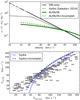Fig. 9 Baryonic effects on the number density of halos. Top panel: the green line is the VF of all galaxies, as measured by ALFALFA (same as in Fig. 3). The green dashed line assumes an incompleteness of the ALFALFA VF at low velocities, parameterized as ${\mathit{f}}_{\mathrm{HI}}^{\mathrm{\left(}\mathrm{2}\mathrm{\right)}}\mathrm{\left(}{\mathit{V}}_{\mathrm{rot}}\mathrm{\right)}$ (see Sect. 4.2). The solid black line represents the VF of halos in the DM-only BolshoiP simulation (also same as in Fig. 3). The dotted black line corresponds to the HVF of halos hosting a stellar counterpart, according to the results of the hydrodynamical simulations of Sawala et al. (2014). The flattening of the hydrodynamical HVF at velocities ≲25 km s-1 is due to the suppression of galaxy formation caused by reionization feedback (see text for details). Bottom panel: the blue dotted line is the average Vrot − Vh relation according to the hydrodynamical result. The dashed blue line additionally takes into account a possible incompleteness of the ALFALFA VF. The gray symbols represent our sample of galaxies with resolved HI rotation curves. These datapoints are slightly shifted with respect to their positions in Fig. 6, because a correction for the cosmic baryon fraction is not necessary when comparing against a hydrodynamical simulation.

In a recent article, Sawala et al. (2014) have explored this issue by means of hydrodynamical simulations. They find that DM-only halos with V_h≲ 70 km s^-1 have larger total masses than their counterparts in more realistic simulations incorporating baryonic physics; they attribute this mass difference to the loss of baryonic material by moderately low-mass halos. Interestingly, they also find that among halos with V_h≲ 25 km s^-1 only a small fraction host a detectable stellar component in the hydrodynamic run. This steep decrease in galaxy formation efficiency for the lowest-mass halos is due to the effects of cosmic reionization. Based on these findings they argue that AM results based on DM-only simulations are not accurate at low velocities.

In order to address these concerns, we re-derive here an average V_rot − V_h relation taking into account the baryonic effects described above. In particular, we use the cumulative HVF of halos that host a stellar counterpart in the hydrodynamic simulations of Sawala et al. (2014). As shown by the top panel of Fig. 9, the hydrodynamic HVF deviates from the HVF of a DM-only simulation at V_h≲ 70 km s^-1, and then flattens out at V_h≲ 25 km s^-1.

We then match the hydrodynamical HVF with the measured galactic VF measured by ALFALFA. The result is shown in the bottom panel of Fig. 9: even in the hydrodynamical case, the V_rot − V_h relation is not very different from the DM-only relation. This is because the number of halos exceeds the number of galaxies already at V_h≈ 35 km s^-1, in a regime where reionization is not yet effective (see top panel). As a result, the discrepancy between the AM relation and the internal kinematics of low-velocity dwarfs seems to persist, even when baryonic effects on the abundance of halos are considered.

The discrepancy is still present, even though somewhat alleviated, if one additionally assumes a substantial incompleteness of the ALFALFA VF (see bottom panel of Fig. 9). A similar result for the V_rot − V_h relation is also obtained when one considers the galactic VF measured by Klypin et al. (2014) in the Local Volume.

4.4. Baryonic effects on dwarf galaxy rotation curves?

Recent results from hydrodynamic simulations of galaxy formation have shown that repeated gas-blowout episodes, driven by bursty star-formation activity, can create a “cored” central DM profile in halos hosting dwarf galaxies (Governato et al. 2012; Pontzen & Governato 2012; but see also Del Popolo et al. 2014 for a different mechanism based on dynamical friction). As already discussed in Sect. 4, Zolotov et al. (2012) argue that accounting for this effect is critical in the context of the satellite TBTF problem (see also Brooks & Zolotov 2014).

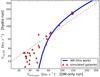Fig. 10 Baryonic effects on galactic rotation curves. The blue solid line is the average Vrot − Vh relation in a ΛCDM universe (same as in Fig. 4). The red triangles represent galaxies from a set of hydrodynamic simulations which include efficient baryonic feedback (Governato et al. 2012; Brooks & Zolotov 2014; Christensen et al. 2014). Simulated low-velocity galaxies fall in the same region of the Vrot − Vh diagram as the actual dwarfs plotted in Fig. 6. This demonstrates that baryonic modifications of the galaxies’ rotation curves do not significantly affect the simplified analysis performed in this work.

Here we try to assess whether baryonic modifications to the RC of low-mass halos can affect the main result of this work. To this end, we place on the V_rot − V_h diagram 28 galaxies produced in an ensemble of hydrodynamical simulations (Governato et al. 2012; Brooks & Zolotov 2014; Christensen et al. 2014); these are shown in Fig. 10. It is worth noting that the values of V_rot and V_h plotted here for the simulated objects have the same definition as for the AM analysis: V_rot is directly measured from simulated edge-on HI profiles (as per Fig. 1), and V_h is the maximum circular velocity of the host halo in the DM-only version of the simulation.

Low-velocity simulated galaxies share the same locus on the V_rot − V_h diagram as the observed dwarf galaxies. This is a crucial point, because it shows that the simplified kinematic analysis performed in this article (based on NFW profiles motivated by DM-only simulations) agrees with the results of the hydrodynamic simulations (which include DM profile modification by baryonic feedback). In particular, simulated galaxies with V_rot≲ 25 km s^-1 lie systematically to lower V_h values than predicted by the AM relation; this placement suggests that the number density of galaxies in the hydrodynamical simulation will be higher than what measured by ALFALFA. This statement is of course true only as long as the effects described in Sects. 4.1–4.3 are in the range explored in this work.

Before we conclude this section we would like to issue a few cautionary notes. First, the comparison between actual and simulated galaxies is only valid provided that the latter have realistic HI properties. Most importantly, simulated galaxies should have HI disk sizes similar to the ones measured in actual dwarfs. However, due to the fact that the HI data for the Governato/Brooks/Christensen et al. simulation sets are not publicly available at present, this analysis is deferred for a future publication (Brooks & Papastergis, in prep.). Second, the main conclusions of this section are drawn based on the results of the specific simulation sets considered here. We cannot therefore exclude the possibility that different simulations – or even the same simulations carried out with different feedback prescriptions – may give substantially different results (for example, cf. Brook & Di Cintio 2014).

4.5. Alternative dark matter models?

Besides baryonic effects, several alternative DM models have been considered to provide solutions to the small-scale challenges faced by ΛCDM. Perhaps the most well studied among them is the warm dark matter (WDM) model, characterized by a DM particle with mass in the ~keV range. Such “light” particles (compared to m_CDM ~ 10 GeV−1 TeV) result in a suppression of structure on spatial scales that are relevant for galaxy formation (e.g., Zavala et al. 2009; Menci et al. 2012). This property of WDM has been regarded as a natural way to resolve CDM overabundance issues. For example, several authors have argued that a WDM model with m_WDM ≈ 1 keV could plausibly reproduce the flatness of the velocity function (e.g., Zavala et al. 2009; Zwaan et al. 2010; Papastergis et al. 2011). In addition, a WDM model with m_WDM = 1.5−2 keV could potentially provide a solution to the satellite TBTF problem (e.g., Lovell et al. 2012; Schneider et al. 2014); this is because MW-sized halos in WDM have fewer – and less dense – massive subhalos compared to CDM.

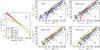Fig. 11 Vrot − Vh diagrams in WDM cosmologies. Panel a) the blue solid line corresponds to the cumulative halo velocity function in a CDM model (same as black solid line in Fig. 3). The red, orange and yellow solid lines correspond to WDM models with particle masses of 4 keV, 2 keV and 1 keV, respectively (Schneider et al. 2014). The dotted green line is the cumulative VF for galaxies of all morphological types (same as solid green line in Fig. 3). Panels b)–e) the colored solid lines correspond to the Vrot − Vh relations in each dark matter model (same color coding as in panel a), inferred by AM. The gray datapoints represent our sample of literature galaxies with HI rotation curves. The same galaxy can be assigned a different value of Vh in each of the four panels, because each model has a different median mass-concentration relation (Schneider et al. 2012).

Here we assess whether WDM can also provide a solution to the field TBTF problem. Panel a of Fig. 11 compares the cumulative HVF of CDM with the corresponding distributions for three WDM models, with m_WDM = 1, 2 and 4 keV. The halo counts for the WDM models have been obtained from the simulations of Schneider et al. (2014). The figure clearly shows that, as m_WDM decreases, the number density of low-velocity halos becomes increasingly more suppressed with respect to CDM. The difference in the cumulative HVFs translates then into different inferred V_rot − V_h relations for each model; the latter are shown in panels b–e of Fig. 11. At the same time, the typical concentration of halos in WDM models is lower than in CDM. In order to place galaxies on the V_rot − V_h diagram for each WDM model, we repeat the process described in Sect. 3.2 using each time the appropriate median c-M_vir relation (Schneider et al. 2012, Eq. (39)). Generally, a given galactic RC can accommodate a progressively more massive host halo, as m_WDM decreases.

Panel e shows that the AM relation predicted by the 1 keV model seems to be fully consistent⁶ with the upper limits derived from individual galaxies. The reason is that both WDM effects discussed above (suppression of the number of low-mass halos & lower halo concentrations) are very pronounced in this model. On the other hand, these same effects are much less prominent in the 2 keV case, even though they are still clearly discernible. Panel d shows that low-velocity galaxies are not fully consistent with the predicted V_rot − V_h relation, even for a model with a particle mass as low as m_WDM = 2 keV. Nonetheless, the inconsistency is significantly alleviated in this case, and perhaps accounting for any of the uncertainties in Sects. 4.1–4.4 could be sufficient to fully resolve the tension.

Despite their promise, WDM models with particle masses in the range 1–2 keV are at odds with a number of independent constraints (at least when interpreted as thermal relics). For example, measurements of the small-scale power of the Ly-α forest at high-z place a 2σ lower limit of m_WDM> 3.3 keV (Viel et al. 2013). In addition, WDM models with m_WDM< 2.3 keV are ruled out by the number of ultra-faint satellites observed around the MW (e.g., Polisensky & Ricotti 2011). As panel c shows, WDM models that do not violate the constraints mentioned above are practically indistinguishable from CDM. For example, in the 4 keV case galaxies with V_rot≲ 25 km s^-1 are clearly incompatible with the predicted AM relation. We therefore conclude that it is unlikely that (thermal relic) WDM can provide a solution to the field TBTF problem, without violating other independent astrophysical constraints.

5. Summary

We measure the distribution of galactic rotational velocities in the nearby universe, using the dataset of the ALFALFA 21 cm survey. Based on the measured velocity function (VF), we statistically connect galaxies with their host halos via the technique of abundance matching (AM). In a ΛCDM universe, linewidth-derived rotational velocities (V_rot,HI) of dwarf galaxies are expected to underestimate the maximum rotational velocity of their host halos (V_h,max). For example, galaxies with V_rot,HI≈ 15 km s^-1 are expected to be hosted by halos with V_h,max≳ 40 km s^-1 (see Fig. 4). This trend reflects the fact that, at the low end, the halo velocity function (HVF) in ΛCDM rises much faster than the observed galactic VF (see Fig. 3).

We then compile an up-to-date literature sample of galaxies with HI rotation curves, to observationally test the predicted V_rot − V_h relation. Our sample contains a large number of extremely low-velocity dwarfs, mainly drawn from the FIGGS, SHIELD and LITTLE THINGS samples. For each galaxy we find the most massive NFW halo that is compatible with the last measured point (LMP) of the galactic rotation curve. Galaxies can then be placed on the V_rot − V_h diagram as upper limits in V_h (see Fig. 5). As Fig. 6 shows, the upper limits derived from individual galaxies are consistent with the average AM relation, for most of the range in galactic rotational velocities (30 km s^-1 ≲ V_rot ≲ 300 km s^-1). Most importantly however, this is not the case for the lowest velocities probed: for example, at V_rot,HI≲ 25 km s^-1 the HI rotation curves of galaxies cannot accommodate host halos as massive as predicted by ΛCDM. This work therefore confirms the similar results previously found for field galaxies by Ferrero et al. (2012) and for non-satellite galaxies in the Local Group by Kirby et al. (2014) & Garrison-Kimmel et al. (2014). At the same time, the analysis performed in this work addresses several caveats present in these previous studies (see Sect. 4).

The discrepancy described above is directly analogous to the too big to fail problem (TBTF) faced by the bright satellites of the Milky Way, but here is observed for galaxies in the field. This finding has therefore important implications, because several of the proposed solutions to the satellite TBTF problem are not applicable in this case. For example, the galaxy population studied in this work mainly consists of gas-rich, fairly isolated objects, that have not been heavily affected by processes such as tidal stripping. As a result, potential solutions to the TBTF problem that rely on strong environmental effects (e.g., Zolotov et al. 2012) cannot explain the presence of a similar discrepancy in the field.

We furthermore consider a number of assumptions and sources of uncertainty that may impact the main conclusions of this work. These include, for example, observational uncertainties on the measurement of the VF and effects related to the bias of HI surveys against gas-poor galaxies. Perhaps the two most important among them, however, are baryonic modifications to the abundance of galaxy-hosting halos and to the velocity profiles of dwarf galaxies. We show that the former baryonic effect does not seem to be able to resolve the reported discrepancy, at least when considered on its own (Sect. 4.3). Furthermore, a preliminary analysis of a set of hydrodynamical simulations (Governato et al. 2012; Brooks & Zolotov 2014; Christensen et al. 2014) suggests that the latter effect is not able to resolve the discrepancy, as well (Sect. 4.4). At the same time, it is still possible that combinations of several of the effects mentioned above may prove sufficient to provide a solution. It is also possible that the baryonic effects considered here may be larger than indicated by the theoretical models used in this work.

Lastly, we check whether an alternative warm dark matter (WDM) model can provide a solution to the field TBTF problem. We find that the inconsistency is lifted in WDM models with particle masses of ≈1 keV. However, (thermal relic) particles with such light masses are in conflict with a number of independent observational constraints (see Sect. 4.5 for details).

Acknowledgments

The authors would like to thank an anonymous referee for their constructive comments and the language editor for their thorough work. The authors would particularly like to thank John Cannon, SeHeon Oh and Alyson Brooks for sharing their yet-to-be-published data. Erwin de Blok, John Cannon, Alyson Brooks, Thijs van der Hulst, Mike Boylan-Kolchin, Marla Geha, Tjitske Starkenburg and Mike Jones provided insightful feedback and comments. E.P. would also like to thank the Aspen Center for Physics for its hospitality (ACP is supported by NSF grant 1066293), and Mary Gooding for her valuable advice. E.P. is supported by a NOVA postdoctoral fellowship at the Kapteyn Institute. The ALFALFA team at Cornell is supported by U.S. NSF grant AST-1107390 to M.P.H. and R.G. and by grants from the Brinson Foundation.

References

Appendix A: Details on the measurement of the velocity function

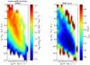Fig. A.1 ALFALFA mass-width function. Left panel: the colormap represents the mass-width function (MWF) measured by ALFALFA, i.e., the number density of galaxies within logarithmic bins of HI mass (MHI) and velocity width (W). The measurement spans the range MHI = 107−1011 M⊙ and W = 28−900 km s-1. Note that the stretch of the colormap is logarithmic. Right panel: colormap of the 1σ statistical error on the number density, expressed in dex (i.e., ${\mathit{\sigma }}_{\log \hspace{0.17em}\mathit{n}}\mathrm{=}\frac{{\mathit{\sigma }}_{\mathit{n}}\mathit{/}\mathit{n}}{\ln \mathrm{\left(}\mathrm{10}\mathrm{\right)}}$). The plotted errors are just due to counting statistics, and systematic uncertainties are not included.

In order to measure galactic number densities as accurately as possible, we apply well-defined selection rules and quality cuts to the α.40 sample. In particular:

• Sources are selected from two rectangular sky regions of the α.40 footprint, which span the same RA range of 08^h00^m<α< 16^h20^m and the Dec ranges 4°<δ< 16° and 24°<δ< 28°, respectively. Both regions are located in the northern Galactic cap, and have almost complete overlap with the SDSS DR7 footprint.

• Only confidently detected ALFALFA sources that are classified as extragalactic objects are considered. In particular, only sources designated as “Code 1” in α.40 and detected at (S/N)_HI> 6.5 are included in the sample.

• Only ALFALFA sources that are crossmatched with a photometric object in the SDSS DR7 are selected. This criterion aims at removing HI sources that are unlikely to be hosted by their own individual halo, such as tidal HI clouds or diffuse gas found in the vicinity of interacting systems. Bona fide galaxies detected by ALFALFA that lack a photometric counterpart in SDSS images are instead extremely rare⁷ (see Sect. 4.3 in Haynes et al. 2011).

• A minimum distance cutoff is imposed at D_min = 7 Mpc. This minimum distance limit is imposed in order to exclude from the sample objects that have a very large uncertainty on their distance, and can therefore introduce large errors in the measurement. At the same time however, this cutoff will exclude some genuinely very low-mass galaxies that can only be detected locally. The distances adopted here are the ones listed in the α.40 catalog, which are primarily based on the flow model of Masters (2005; for details refer to Sect. 3.2 in Martin et al. 2010). Keep in mind that flow model distances for very nearby objects can have large fractional errors (see e.g., McQuinn et al. 2014). In general, distance uncertainties result in an overestimate of the number density of low-velocity galaxies, even though the effect is not large (Papastergis et al. 2011, Sect. 4.2). A maximum distance cutoff is defined in terms of recessional velocity in the CMB frame of reference, as cz_max = 15 000 km s^-1 (D_max ≈ 214 Mpc). This maximum recessional velocity limit is imposed in order to avoid a spectral region that is heavily affected by radio frequency interference.

• HI sources that lie below the 50% completeness limit of the ALFALFA survey are excluded from the sample. The completeness limit of the ALFALFA survey has been measured in Sect. 6 of Haynes et al. (2011). In this work we use Eqs. (4) and (5) in Haynes et al. (2011), to define the flux values corresponding to 50% completeness as a function of velocity width⁸.

• We restrict our sample to the HI mass range of M_HI = 10⁷−10¹¹ M_⊙ and the velocity width range of W₅₀ = 28−900 km s^-1. These lower bounds on HI mass and velocity width are conservative, and do not reflect the performance limitations of the ALFALFA survey.

The above set of selection rules results in a final sample of 6770 sources, located over ≈2900 deg² of sky and within a volume of approximately 2 × 10⁶ Mpc³. This is the sample used to calculate the mass-width function (MWF) of galaxies, shown in the left panel of Fig. A.1. The horizontal axis of the panel is the rest frame velocity width, W, which is derived from the observed velocity width, W₅₀, after a Doppler broadening correction is applied: W = W₅₀/ (1 + z_⊙). The vertical axis is HI mass, M_HI, calculated from a source’s HI flux, S_HI, and distance, D, through the relation M_HI(M_⊙) = 235.6 × S_HI(mJykm s^-1) × D²(Mpc). The color scale shows the number density of galaxies within logarithmic bins in M_HI and W, i.e., 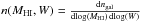$\mathit{n}\mathrm{\left(}{\mathit{M}}_{\mathrm{HI}}\mathit{,W}\mathrm{\right)}\mathrm{=}\frac{\mathrm{d}{\mathit{n}}_{\mathrm{gal}}}{\mathrm{d}\log \mathrm{\left(}{\mathit{M}}_{\mathrm{HI}}\mathrm{\right)}\hspace{0.17em}\mathrm{d}\log \mathrm{\left(}\mathit{W}\mathrm{\right)}}$. The right panel of Fig. A.1 shows the error on the number density, expressed in dex (i.e., ${\mathit{\sigma }}_{\log \hspace{0.17em}\mathit{n}}\mathrm{=}\frac{{\mathit{\sigma }}_{\mathit{n}}\mathit{/}\mathit{n}}{\ln \mathrm{\left(}\mathrm{10}\mathrm{\right)}}$). The error plotted here only includes the uncertainty from counting statistics, and is therefore lowest in the mass-width bins with the highest number of detections (and vice-versa). Several other sources of uncertainty, most of them systematic, are not included in the errors above (see however discussion in Sect. 4.1).

Since the ALFALFA sample is not volume-limited, the MWF shown in Fig. A.1 is not just a simple number count of detections normalized by the survey volume. In particular, galaxies with different masses and widths can be detected over different volumes, so each source has to be weighted by an appropriate volume-correction factor. In this work, we calculate weighting factors via the “1 /V_eff” maximum-likelihood method. A thorough description of the method and full details of its implementation can be found in Papastergis et al. (2011) and Zwaan et al. (2010) and references therein, but here we very briefly summarize its most important characteristics: For each galaxy i in the final sample we calculate an “effective” volume, V_eff,i, which depends on the object’s HI mass, velocity width and distance (M_HI,i, W_50,i & D_i, respectively). The value of the MWF in mass bin j and width bin k and its corresponding “counting” error can then be calculated as 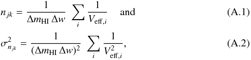$\begin{array}{ccc}& & {\mathit{n}}_{\mathit{jk}}\mathrm{=}\frac{\mathrm{1}}{\mathrm{\Delta }{\mathit{m}}_{\mathrm{HI}}\hspace{0.17em}\mathrm{\Delta }\mathit{w}}\sum _{\mathit{i}}\frac{\mathrm{1}}{{\mathit{V}}_{\mathrm{eff}\mathit{,i}}}\mathrm{and}\\ & & {\mathit{\sigma }}_{{\mathit{n}}_{\mathit{jk}}}^{\mathrm{2}}\mathrm{=}\frac{\mathrm{1}}{\mathrm{(}\mathrm{\Delta }{\mathit{m}}_{\mathrm{HI}}\hspace{0.17em}\mathrm{\Delta }\mathit{w}{\mathrm{)}}^{\mathrm{2}}}\sum _{\mathit{i}}\frac{\mathrm{1}}{{\mathit{V}}_{\mathrm{eff}\mathit{,i}}^{\mathrm{2}}}\mathit{,}\end{array}$where the summation runs over all galaxies i which belong to the specific bin. In the equations above, Δm_HI and Δw are the sizes of the logarithmic bins in mass and width (i.e., m_HI = log (M_HI/M_⊙) and w = log (W/ km s^-1)). The equations above have the same form as the equations used in the standard “1 /V_max” method. In the 1 /V_max case, the quantity entering Eq. (A.1) would be V_max,i, which is defined as the maximum volume over which galaxy i can be detected according to the survey sensitivity. In fact, V_eff,i exactly coincides with V_max,i for a spatially homogeneous sample. The advantage of the 1 /V_eff method is that it takes into account density fluctuations in the survey volume, and therefore the resulting estimates are less susceptible to biases introduced by the presence of large-scale structure.

If we marginalize the two-dimensional MWF along each axis in turn, we obtain the HI mass function (HIMF) and the velocity width function (WF) of galaxies. These distributions are of central importance in extragalactic astronomy, and their measurement and scientific interpretation has been the subject of a large body of literature (see e.g., Martin et al. 2010; Zwaan et al. 2005, 2010; Papastergis et al. 2011 for some of the most recent observational results).

Appendix B: Last measured point (LMP) radii and velocities for dwarf galaxy sample

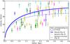Fig. B.1 Last measured point radii and velocities for dwarf galaxies. The datapoints represent the radii and velocities at the LMP for some of the galaxies with resolved HI observations (Sect. 3.1). This plot is restricted to VLMP< 50 km s-1, where most of the “failing” extreme dwarf galaxies in Fig. 6 are found. The datapoints are color coded according to their original data reference, same as in Fig. 6. The three blue lines represent the RCs of NFW halos that are assigned through AM to galaxies with Vrot = 15 km s-1. In particular, the solid line represents the fiducial AM result (Fig. 6), the dotted line represents the AM result including baryonic effects on the abundance of halos, and the dashed line represents the AM result including baryonic effects on the abundance of halos and observational incompleteness of the ALFALFA VF (see Fig. 9).

Figure B.1 shows the radii and velocities at the LMP for a subset of the interferometric galaxy sample described in Sect. 3.1. In particular, the figure zooms on the range R_LMP< 4.5 kpc and V_LMP< 50 km s^-1, where most of the “failing” dwarfs of Fig. 6 reside. Where appropriate, the plotted V_LMP values have been corrected for the effects of turbulent motions (see Sect. 3.3).

For reference, we also plot the RC of halos that are assigned through AM to a galaxy with V_rot = 15 km s^-1. In particular, the solid RC represents our fiducial AM analysis (Sect. 2.2 and Fig. 6), the dotted RC represents the AM analysis including baryonic effects on the abundance of halos (Sect. 4.3 and Fig. 9), and lastly the dashed RC refers to the AM analysis including baryonic effects and observational incompleteness of the ALFALFA VF (also Sect. 4.3 and Fig. 9). We note that the solid RC has been rescaled down according to the cosmic baryon fraction (see discussion in Sect. 3.2); as a result, the difference between the solid and dotted RCs reflects baryonic effects on the abundances of halos that are in addition to a simple rescaling.

Since 15 km s^-1 is approximately the lowest value of V_rot encountered in our sample, these halos are effectively the smallest halos that are expected to host galaxies according to each AM result. Consequently, galaxies whose LMP measurement lies below each of the plotted RCs, are (almost certainly) a “failure” in Fig. 6. At the same time, Fig. B.1 shows that most failing dwarfs have R_LMP ≲ 3 kpc. As a result, baryonic modifications to the inner velocity profiles of halos should be taken into account when interpreting the results of this article. Figure B.1 also illustrates the point that baryonic modifications to the RCs of halos can only resolve the issue if baryonic feedback can have a sizable impact at radii as large as 2–3 kpc. However, the preliminary analysis of hydrodynamic simulations described in Sect. 4.4 suggests that this is not the case (but keep also in mind cautionary notes in Sect. 4.4).

All Figures

Fig. 1 HI-line profiles for three representative ALFALFA sources. For each galaxy the velocity width, W50, is measured between the two outermost points where the flux density falls to 50% of the peak value (red vertical lines). Left panel: MW analog with a typical “double horned” profile, indicative of a mostly flat outer rotation curve. Central panel: dwarf galaxy with a “boxy” profile shape. Right panel: extreme dwarf galaxy with a clearly “single-peaked” profile, suggestive of a rising rotation curve. Keep in mind that narrow profiles can also correspond to intrinsically high-width objects that are oriented close to face-on. Note also that the velocity span of the x-axis in all three panels is the same (1800 km s-1), and so profile widths are plotted to scale.

In the text

Fig. 2 ALFALFA measurement of the width and rotational velocity functions. Top panel: data points represent the velocity width function (WF) of galaxies measured by ALFALFA, for galaxies with . The errorbars represent the 1σ counting noise (see Eq. (A.1)), and do not include any systematic uncertainties. The dotted line is a modified Schechter fit to the data (Eq. (1)), with parameters: $\log \mathrm{\left(}{\mathit{n}}_{\mathrm{\ast }}\mathrm{\right)}\mathrm{=}\mathrm{-}\mathrm{1.68}\mathrm{\pm }\mathrm{0.20}\hspace{0.17em}{\mathit{h}}_{\mathrm{70}}^{\mathrm{3}}{\mathrm{Mpc}}^{-3}\hspace{0.17em}{\mathrm{dex}}^{-1}$, log (W∗) = 2.52 ± 0.076 km s-1, α = −0.45 ± 0.24 and β = 2.39 ± 0.50. Bottom panel: data points represent the rotational velocity function (VF) of galaxies measured by ALFALFA, again for galaxies with . Rotational velocities, Vrot, have been obtained from inclination-corrected velocity widths according to Eq. (2). Errorbars again represent the 1σ counting noise, and do not include any systematic uncertainties. The dotted line is a modified Schechter fit to the data, with parameters: $\log \mathrm{\left(}{\mathit{n}}_{\mathrm{\ast }}\mathrm{\right)}\mathrm{=}\mathrm{-}\mathrm{1.17}\mathrm{\pm }\mathrm{0.25}{\mathit{h}}_{\mathrm{70}}^{\mathrm{3}}{\mathrm{Mpc}}^{-3}\hspace{0.17em}{\mathrm{dex}}^{-1}$, log (V∗) = 2.04 ± 0.18 km s-1, α = 0.14 ± 0.41 and β = 1.46 ± 0.37.

In the text

Fig. 3 Cumulative velocity functions for galaxies and ΛCDM halos. The dashed black line represents the cumulative number density of halos as a function of their maximum circular velocity, Vh, in a ΛCDM universe (BolshoiP simulation; Hess et al., in prep.). The solid black line corresponds to the “galactic” HVF, which excludes massive halos that are unlikely to host individual galaxies (see Eq. (5)). The dotted green line shows the cumulative VF of ALFALFA galaxies. The red shaded region represents the VF of early-type galaxies, measured from SDSS data (Bernardi et al. 2010). The solid green line represents the VF of galaxies of all morphological types, obtained from the sum of the ALFALFA and early-type VFs.

In the text

Fig. 4 Vrot − Vh relation in a ΛCDM universe. The blue line is the average relation between the galactic HI rotational velocity (Vrot) and the maximum circular velocity of the host halo (Vh), in a ΛCDM universe. This relation is obtained by abundance matching (AM), i.e., by matching the cumulative velocity distributions of all galaxies and “galactic” halos (see Fig. 3). The dashed blue line is the AM result when galaxies are matched to all halos. The dashed black line is a reference one-to-one line.

In the text

Fig. 5 Kinematic analysis of galaxies with HI rotation curves. Top panel: three representative rotation curves (RCs) from the literature sample of galaxies with interferometric HI observations (red: UGC 7577, green: UGC 7323; blue: UGC 8490). The gray solid lines show the RCs of increasingly more massive NFW halos (from bottom to top). The concentration parameter for each halo is the median concentration expected for its mass in a Planck cosmology (Dutton & Macciò 2014). The three thick gray lines show the most massive NFW halos that are compatible with the last measured point of each galaxy’s RC (large colored symbols), to within 1σ. For each galaxy, only the last measured point of the RC is used for the analysis in this work. The peak velocity for each of these three halos is the value of Vh assigned to the corresponding galaxy. The colored horizontal marks denote the value of Vrot for the three galaxies, inferred from their inclination-corrected linewidths (see Eq. (2)). Bottom panel: small circles show the placement of UGC 7577, UGC 7323 and UGC 8490 on the Vrot − Vh diagram, according to the procedure outlined in the top panel. The large diamonds show their positions after a correction is applied to account for the cosmic baryon fraction (see text for details).

In the text

Fig. 6 Placement of galaxies on the Vrot − Vh diagram. Main figure: the blue line is the average Vrot − Vh relation in a ΛCDM universe, inferred from abundance matching (same as in Fig. 4). The colored points represent a sample of 194 galaxies with interferometric HI observations, drawn from the literature. Their Vrot and Vh values are computed as described in Fig. 5. All points are drawn as upper limits, because we make the conservative assumption that the contribution of baryons to the galactic RC is negligible for all galaxies. Refer to Sects. 3.3 and 4 for the scientific interpretation of this figure. Inset panel: a zoom-in on the low-velocity region of the diagram (linear axes).

In the text

Fig. 7 Observational uncertainties on the VF measurement. Top panel: the blue shaded region shows the range of ALFALFA cumulative VFs that correspond to modified Schechter parameters within 1σ from the best fit values (see Eq. (1)). The cyan line corresponds to the result of the HIPASS 21 cm survey (Zwaan et al. 2010), while the red line represents the cumulative VF measured in the Local Volume by Klypin et al. (2014). The two latter results are plotted to illustrate the magnitude of systematic uncertainties affecting the measurement of the VF. Bottom panel: the gray symbols represent our sample of galaxies with literature HI rotation curves (same as in Fig. 6). The colored lines represent the Vrot − Vh relation that corresponds to each of the cumulative VFs plotted in the upper panel, using the same color coding.

In the text

Fig. 8 Incompleteness of the ALFALFA survey at low velocities. Top panel: the blue dotted, dashed and dash-dotted lines represent three relations for the “HI-selection” factor, fHI(Vrot), each accounting for progressively more low-velocity systems that are undetectable by ALFALFA due to their low HI mass (Eqs. (9)–(11)). Bottom panel: the blue dotted, dashed and dash-dotted lines are the average Vrot − Vh relations for the corresponding fHI(Vrot) relations shown in the top panel. For reference, we also plot our fiducial relation with a thick solid blue line (same as in Fig. 4). The gray symbols represent our sample of galaxies with HI rotation curves, same as in Fig. 6.

In the text

Fig. 9 Baryonic effects on the number density of halos. Top panel: the green line is the VF of all galaxies, as measured by ALFALFA (same as in Fig. 3). The green dashed line assumes an incompleteness of the ALFALFA VF at low velocities, parameterized as ${\mathit{f}}_{\mathrm{HI}}^{\mathrm{\left(}\mathrm{2}\mathrm{\right)}}\mathrm{\left(}{\mathit{V}}_{\mathrm{rot}}\mathrm{\right)}$ (see Sect. 4.2). The solid black line represents the VF of halos in the DM-only BolshoiP simulation (also same as in Fig. 3). The dotted black line corresponds to the HVF of halos hosting a stellar counterpart, according to the results of the hydrodynamical simulations of Sawala et al. (2014). The flattening of the hydrodynamical HVF at velocities ≲25 km s-1 is due to the suppression of galaxy formation caused by reionization feedback (see text for details). Bottom panel: the blue dotted line is the average Vrot − Vh relation according to the hydrodynamical result. The dashed blue line additionally takes into account a possible incompleteness of the ALFALFA VF. The gray symbols represent our sample of galaxies with resolved HI rotation curves. These datapoints are slightly shifted with respect to their positions in Fig. 6, because a correction for the cosmic baryon fraction is not necessary when comparing against a hydrodynamical simulation.

In the text

Fig. 10 Baryonic effects on galactic rotation curves. The blue solid line is the average Vrot − Vh relation in a ΛCDM universe (same as in Fig. 4). The red triangles represent galaxies from a set of hydrodynamic simulations which include efficient baryonic feedback (Governato et al. 2012; Brooks & Zolotov 2014; Christensen et al. 2014). Simulated low-velocity galaxies fall in the same region of the Vrot − Vh diagram as the actual dwarfs plotted in Fig. 6. This demonstrates that baryonic modifications of the galaxies’ rotation curves do not significantly affect the simplified analysis performed in this work.

In the text

Fig. 11 Vrot − Vh diagrams in WDM cosmologies. Panel a) the blue solid line corresponds to the cumulative halo velocity function in a CDM model (same as black solid line in Fig. 3). The red, orange and yellow solid lines correspond to WDM models with particle masses of 4 keV, 2 keV and 1 keV, respectively (Schneider et al. 2014). The dotted green line is the cumulative VF for galaxies of all morphological types (same as solid green line in Fig. 3). Panels b)–e) the colored solid lines correspond to the Vrot − Vh relations in each dark matter model (same color coding as in panel a), inferred by AM. The gray datapoints represent our sample of literature galaxies with HI rotation curves. The same galaxy can be assigned a different value of Vh in each of the four panels, because each model has a different median mass-concentration relation (Schneider et al. 2012).

In the text

Fig. A.1 ALFALFA mass-width function. Left panel: the colormap represents the mass-width function (MWF) measured by ALFALFA, i.e., the number density of galaxies within logarithmic bins of HI mass (MHI) and velocity width (W). The measurement spans the range MHI = 107−1011 M⊙ and W = 28−900 km s-1. Note that the stretch of the colormap is logarithmic. Right panel: colormap of the 1σ statistical error on the number density, expressed in dex (i.e., ${\mathit{\sigma }}_{\log \hspace{0.17em}\mathit{n}}\mathrm{=}\frac{{\mathit{\sigma }}_{\mathit{n}}\mathit{/}\mathit{n}}{\ln \mathrm{\left(}\mathrm{10}\mathrm{\right)}}$). The plotted errors are just due to counting statistics, and systematic uncertainties are not included.

In the text

Fig. B.1 Last measured point radii and velocities for dwarf galaxies. The datapoints represent the radii and velocities at the LMP for some of the galaxies with resolved HI observations (Sect. 3.1). This plot is restricted to VLMP< 50 km s-1, where most of the “failing” extreme dwarf galaxies in Fig. 6 are found. The datapoints are color coded according to their original data reference, same as in Fig. 6. The three blue lines represent the RCs of NFW halos that are assigned through AM to galaxies with Vrot = 15 km s-1. In particular, the solid line represents the fiducial AM result (Fig. 6), the dotted line represents the AM result including baryonic effects on the abundance of halos, and the dashed line represents the AM result including baryonic effects on the abundance of halos and observational incompleteness of the ALFALFA VF (see Fig. 9).

In the text

References

- Adams, E. A. K., Giovanelli, R., & Haynes, M. P. 2013, ApJ, 768, 77 [NASA ADS] [CrossRef] [Google Scholar]
- Arraki, K. S., Klypin, A., More, S., & Trujillo-Gomez, S. 2014, MNRAS, 438, 1466 [NASA ADS] [CrossRef] [Google Scholar]
- Baes, M., Buyle, P., Hau, G. K. T., & Dejonghe, H. 2003, MNRAS, 341, L44 [NASA ADS] [CrossRef] [Google Scholar]
- Baldry, I. K., Glazebrook, K., & Driver, S. P. 2008, MNRAS, 388, 945 [NASA ADS] [Google Scholar]
- Baldry, I. K., Driver, S. P., Loveday, J., et al. 2012, MNRAS, 421, 621 [NASA ADS] [Google Scholar]
- Begum, A., Chengalur, J. N., Karachentsev, I. D., Sharina, M. E., & Kaisin, S. S. 2008a, MNRAS, 386, 1667 [NASA ADS] [CrossRef] [Google Scholar]
- Begum, A., Chengalur, J. N., Karachentsev, I. D., & Sharina, M. E. 2008b, MNRAS, 386, 138 [NASA ADS] [CrossRef] [Google Scholar]
- Bernardi, M., Shankar, F., Hyde, J. B., et al. 2010, MNRAS, 404, 2087 [NASA ADS] [Google Scholar]
- Bernstein-Cooper, E. Z., Cannon, J. M., Elson, E. C., et al. 2014, AJ, 148, 35 [NASA ADS] [CrossRef] [Google Scholar]
- Boylan-Kolchin, M., Bullock, J. S., & Kaplinghat, M. 2011, MNRAS, 415, L40 [CrossRef] [Google Scholar]
- Boylan-Kolchin, M., Bullock, J. S., & Kaplinghat, M. 2012, MNRAS, 422, 1203 [NASA ADS] [CrossRef] [Google Scholar]
- Brook, C. B., & Di Cintio, A. 2014, MNRAS, submitted [arXiv:1410.3825] [Google Scholar]
- Brooks, A. M., & Zolotov, A. 2014, ApJ, 786, 87 [NASA ADS] [CrossRef] [Google Scholar]
- Bullock, J. S., Kravtsov, A. V., & Weinberg, D. H. 2000, ApJ, 539, 517 [NASA ADS] [CrossRef] [Google Scholar]
- Cannon, J. M., Giovanelli, R., Haynes, M. P., et al. 2011, ApJ, 739, L22 [NASA ADS] [CrossRef] [Google Scholar]
- Christensen, C. R., Governato, F., Quinn, T., et al. 2014, MNRAS, 440, 2843 [NASA ADS] [CrossRef] [Google Scholar]
- Collins, M. L. M., Chapman, S. C., Rich, R. M., et al. 2013, ApJ, 768, 172 [NASA ADS] [CrossRef] [Google Scholar]
- Côté, S., Carignan, C., & Freeman, K. C. 2000, AJ, 120, 3027 [NASA ADS] [CrossRef] [Google Scholar]
- de Blok, W. J. G., Walter, F., Brinks, E., et al. 2008, AJ, 136, 2648 [NASA ADS] [CrossRef] [Google Scholar]
- Del Popolo, A., Lima, J. A. S., Fabris, J. C., & Rodrigues, D. C. 2014, J. Cosmol. Astropart. Phys., 4, 21 [Google Scholar]
- Di Cintio, A., Brook, C. B., Macciò, A. V., et al. 2014a, MNRAS, 437, 415 [NASA ADS] [CrossRef] [Google Scholar]
- Di Cintio, A., Brook, C. B., Dutton, A. A., et al. 2014b, MNRAS, 441, 2986 [NASA ADS] [CrossRef] [Google Scholar]
- Dutton, A. A., & Macciò, A. V. 2014, MNRAS, 441, 3359 [NASA ADS] [CrossRef] [Google Scholar]
- Ferrarese, L. 2002, ApJ, 578, 90 [NASA ADS] [CrossRef] [Google Scholar]
- Ferrero, I., Abadi, M. G., Navarro, J. F., Sales, L. V., & Gurovich, S. 2012, MNRAS, 425, 2817 [Google Scholar]
- Garrison-Kimmel, S., Boylan-Kolchin, M., Bullock, J. S., & Kirby, E. N. 2014, MNRAS, 444, 222 [NASA ADS] [CrossRef] [Google Scholar]
- Geha, M., Blanton, M. R., Yan, R., & Tinker, J. L. 2012, ApJ, 757, 85 [NASA ADS] [CrossRef] [Google Scholar]
- Giovanelli, R., Haynes, M. P., Salzer, J. J., et al. 1994, AJ, 107, 2036 [NASA ADS] [CrossRef] [Google Scholar]
- Giovanelli, R., Haynes, M. P., Adams, E. A. K., et al. 2013, AJ, 146, 15 [NASA ADS] [CrossRef] [Google Scholar]
- Governato, F., Brook, C., Mayer, L., et al. 2010, Nature, 463, 203 [NASA ADS] [CrossRef] [PubMed] [Google Scholar]
- Governato, F., Zolotov, A., Pontzen, A., et al. 2012, MNRAS, 422, 1231 [NASA ADS] [CrossRef] [Google Scholar]
- Haynes, M. P., Giovanelli, R., Martin, A. M., et al. 2011, AJ, 142, 170 [NASA ADS] [CrossRef] [Google Scholar]
- Huang, S., Haynes, M. P., Giovanelli, R., & Brinchmann, J. 2012, ApJ, 756, 113 [NASA ADS] [CrossRef] [Google Scholar]
- Hunter, D. A., Ficut-Vicas, D., Ashley, T., et al. 2012, AJ, 144, 134 [NASA ADS] [CrossRef] [Google Scholar]
- Karachentsev, I. D., Makarov, D. I., & Kaisina, E. I. 2013, AJ, 145, 101 [NASA ADS] [CrossRef] [Google Scholar]
- Kirby, E. M., Koribalski, B., Jerjen, H., & López-Sánchez, Á. 2012, MNRAS, 420, 2924 [NASA ADS] [CrossRef] [Google Scholar]
- Kirby, E. N., Bullock, J. S., Boylan-Kolchin, M., Kaplinghat, M., & Cohen, J. G. 2014, MNRAS, 439, 1015 [Google Scholar]
- Klypin, A., Kravtsov, A. V., Valenzuela, O., & Prada, F. 1999, ApJ, 522, 82 [Google Scholar]
- Klypin, A. A., Trujillo-Gomez, S., & Primack, J. 2011, ApJ, 740, 102 [Google Scholar]
- Klypin, A., Karachentsev, I., Makarov, D., & Nasonova, O. 2014, MNRAS, submitted [arXiv:1405.4523] [Google Scholar]
- Kravtsov, A. V., Gnedin, O. Y., & Klypin, A. A. 2004, ApJ, 609, 482 [NASA ADS] [CrossRef] [Google Scholar]
- Li, C., & White, S. D. M. 2009, MNRAS, 398, 2177 [NASA ADS] [CrossRef] [Google Scholar]
- Lovell, M. R., Eke, V., Frenk, C. S., et al. 2012, MNRAS, 420, 2318 [NASA ADS] [CrossRef] [Google Scholar]
- Mainini, R., Macciò, A. V., Bonometto, S. A., & Klypin, A. 2003, ApJ, 599, 24 [NASA ADS] [CrossRef] [Google Scholar]
- Martin, A. M., Papastergis, E., Giovanelli, R., et al. 2010, ApJ, 723, 1359 [NASA ADS] [CrossRef] [Google Scholar]
- Masters, K. L. 2005, Ph.D. Thesis New York, Cornell University [Google Scholar]
- McQuinn, K. B. W., Cannon, J. M., Dolphin, A. E., et al. 2014, ApJ, 785, 3 [NASA ADS] [CrossRef] [Google Scholar]
- Menci, N., Fiore, F., & Lamastra, A. 2012, MNRAS, 421, 2384 [NASA ADS] [CrossRef] [Google Scholar]
- Moore, B., Ghigna, S., Governato, F., et al. 1999, ApJ, 524, L19 [Google Scholar]
- Navarro, J. F., Frenk, C. S., & White, S. D. M. 1997, ApJ, 490, 493 [NASA ADS] [CrossRef] [Google Scholar]
- Obreschkow, D., Croton, D., De Lucia, G., Khochfar, S., & Rawlings, S. 2009, ApJ, 698, 1467 [NASA ADS] [CrossRef] [Google Scholar]
- Obreschkow, D., Ma, X., Meyer, M., et al. 2013, ApJ, 766, 137 [NASA ADS] [CrossRef] [Google Scholar]
- Oh, S.-H., de Blok, W. J. G., Brinks, E., Walter, F., & Kennicutt, R. C., Jr. 2011a, AJ, 141, 193 [NASA ADS] [CrossRef] [Google Scholar]
- Oh, S.-H., Brook, C., Governato, F., et al. 2011b, AJ, 142, 24 [NASA ADS] [CrossRef] [Google Scholar]
- Okamoto, T., Gao, L., & Theuns, T. 2008, MNRAS, 390, 920 [NASA ADS] [CrossRef] [Google Scholar]
- Papastergis, E., Martin, A. M., Giovanelli, R., & Haynes, M. P. 2011, ApJ, 739, 38 [Google Scholar]
- Papastergis, E., Cattaneo, A., Huang, S., Giovanelli, R., & Haynes, M. P. 2012, ApJ, 759, 138 [NASA ADS] [CrossRef] [Google Scholar]
- Papastergis, E., Giovanelli, R., Haynes, M. P., Rodríguez-Puebla, A., & Jones, M. G. 2013, ApJ, 776, 43 [NASA ADS] [CrossRef] [Google Scholar]
- Peebles, P. J. E. 2001, ApJ, 557, 495 [NASA ADS] [CrossRef] [Google Scholar]
- Planck Collaboration XVI. 2014, A&A, 571, A16 [NASA ADS] [CrossRef] [EDP Sciences] [Google Scholar]
- Polisensky, E., & Ricotti, M. 2011, Phys. Rev. D, 83, 043506 [NASA ADS] [CrossRef] [Google Scholar]
- Pontzen, A., & Governato, F. 2012, MNRAS, 421, 3464 [NASA ADS] [CrossRef] [Google Scholar]
- Purcell, C. W., & Zentner, A. R. 2012, J. Cosmol. Astropart. Phys., 12, 7 [Google Scholar]
- Rodríguez-Puebla, A., Avila-Reese, V., Firmani, C., & Colín, P. 2011, Rev. Mex. Astron. Astrofis., 47, 235 [NASA ADS] [Google Scholar]
- Rodríguez-Puebla, A., Avila-Reese, V., & Drory, N. 2013, ApJ, 773, 172 [NASA ADS] [CrossRef] [Google Scholar]
- Rosenberg, J. L., & Schneider, S. E. 2002, ApJ, 567, 247 [NASA ADS] [CrossRef] [Google Scholar]
- Samushia, L., Reid, B. A., White, M., et al. 2013, MNRAS, 429, 1514 [NASA ADS] [CrossRef] [Google Scholar]
- Sanders, R. H. 1996, ApJ, 473, 117 [NASA ADS] [CrossRef] [Google Scholar]
- Sawala, T., Frenk, C. S., Crain, R. A., et al. 2013, MNRAS, 431, 1366 [NASA ADS] [CrossRef] [Google Scholar]
- Sawala, T., Frenk, C. S., Fattahi, A., et al. 2014, MNRAS, submitted [arXiv:1404.3724] [Google Scholar]
- Schneider, A., Smith, R. E., Macciò, A. V., & Moore, B. 2012, MNRAS, 424, 684 [NASA ADS] [CrossRef] [Google Scholar]
- Schneider, A., Anderhalden, D., Macciò, A. V., & Diemand, J. 2014, MNRAS, 441, L6 [Google Scholar]
- Shankar, F., Lapi, A., Salucci, P., De Zotti, G., & Danese, L. 2006, ApJ, 643, 14 [NASA ADS] [CrossRef] [MathSciNet] [Google Scholar]
- Somerville, R. S. 2002, ApJ, 572, L23 [NASA ADS] [CrossRef] [Google Scholar]
- Springel, V., Wang, J., Vogelsberger, M., et al. 2008, MNRAS, 391, 1685 [NASA ADS] [CrossRef] [Google Scholar]
- Strigari, L. E., & Wechsler, R. H. 2012, ApJ, 749, 75 [NASA ADS] [CrossRef] [Google Scholar]
- Swaters, R. A., Sancisi, R., van Albada, T. S., & van der Hulst, J. M. 2009, A&A, 493, 871 [NASA ADS] [CrossRef] [EDP Sciences] [Google Scholar]
- Swaters, R. A., Sancisi, R., van Albada, T. S., & van der Hulst, J. M. 2011, ApJ, 729, 118 [NASA ADS] [CrossRef] [Google Scholar]
- Tollerud, E. J., Boylan-Kolchin, M., & Bullock, J. S. 2014, MNRAS, 440, 3511 [NASA ADS] [CrossRef] [Google Scholar]
- Tikhonov, A. V., & Klypin, A. 2009, MNRAS, 395, 1915 [NASA ADS] [CrossRef] [MathSciNet] [Google Scholar]
- Tinker, J. L., & Conroy, C. 2009, ApJ, 691, 633 [NASA ADS] [CrossRef] [Google Scholar]
- Trachternach, C., de Blok, W. J. G., McGaugh, S. S., van der Hulst, J. M., & Dettmar, R.-J. 2009, A&A, 505, 577 [NASA ADS] [CrossRef] [EDP Sciences] [Google Scholar]
- Trujillo-Gomez, S., Klypin, A., Primack, J., & Romanowsky, A. J. 2011, ApJ, 742, 16 [NASA ADS] [CrossRef] [Google Scholar]
- Trujillo-Gomez, S., Klypin, A., Colin, P., et al. 2015, MNRAS, 446, 1140 [NASA ADS] [CrossRef] [Google Scholar]
- van der Marel, R. P., Fardal, M., Besla, G., et al. 2012, ApJ, 753, 8 [NASA ADS] [CrossRef] [Google Scholar]
- Vera-Ciro, C. A., Helmi, A., Starkenburg, E., & Breddels, M. A. 2013, MNRAS, 428, 1696 [NASA ADS] [CrossRef] [Google Scholar]
- Verheijen, M. A. W., & Sancisi, R. 2001, A&A, 370, 765 [NASA ADS] [CrossRef] [EDP Sciences] [Google Scholar]
- Viel, M., Becker, G. D., Bolton, J. S., & Haehnelt, M. G. 2013, Phys. Rev. D, 88, 043502 [NASA ADS] [CrossRef] [Google Scholar]
- Wang, J., Frenk, C. S., Navarro, J. F., Gao, L., & Sawala, T. 2012, MNRAS, 424, 2715 [NASA ADS] [CrossRef] [Google Scholar]
- Watkins, L. L., Evans, N. W., & An, J. H. 2010, MNRAS, 406, 264 [NASA ADS] [CrossRef] [Google Scholar]
- Zavala, J., Jing, Y. P., Faltenbacher, A., et al. 2009, ApJ, 700, 1779 [NASA ADS] [CrossRef] [Google Scholar]
- Zolotov, A., Brooks, A. M., Willman, B., et al. 2012, ApJ, 761, 71 [Google Scholar]
- Zwaan, M. A., Meyer, M. J., Staveley-Smith, L., & Webster, R. L. 2005, MNRAS, 359, L30 [NASA ADS] [CrossRef] [Google Scholar]
- Zwaan, M. A., Meyer, M. J., & Staveley-Smith, L. 2010, MNRAS, 403, 1969 [NASA ADS] [CrossRef] [Google Scholar]