| Issue |
A&A
Volume 568, August 2014
|
|
|---|---|---|
| Article Number | A30 | |
| Number of page(s) | 6 | |
| Section | The Sun | |
| DOI | https://doi.org/10.1051/0004-6361/201322815 | |
| Published online | 08 August 2014 | |
Reciprocatory magnetic reconnection in a coronal bright point⋆
1
Key Laboratory for Dark Matter and Space Science, Purple Mountain
Observatory, CAS,
210008
Nanjing,
PR China
e-mail:
This email address is being protected from spambots. You need JavaScript enabled to view it.
2
School of Astronomy and Space Science, Nanjing University,
210093
Nanjing, PR
China
3
Key Lab of Modern Astronomy and Astrophysics,
Ministry of
Education, PR China
Received:
8
October
2013
Accepted:
20
June
2014
Abstract
Context. Coronal bright points (CBPs) are small-scale and long-duration brightenings in the lower solar corona. They are often explained in terms of magnetic reconnection.
Aims. We aim to study the substructures of a CBP and clarify the relationship among the brightenings of different patches inside the CBP.
Methods. The event was observed by the X-ray Telescope (XRT) aboard the Hinode spacecraft on 2009 August 22−23.
Results. The CBP showed repeated brightenings (or CBP flashes). During each of the two successive CBP flashes, that is, weak and strong flashes that were separated by ~2 hr, the XRT images revealed that the CBP was composed of two chambers, patches A and B. During the weak flash, patch A brightened first, and patch B brightened ~2 min later. During the transition, the right leg of a large-scale coronal loop drifted from the right side of the CBP to the left side. During the strong flash, patch B brightened first, and patch A brightened ~2 min later. During the transition, the right leg of the large-scale coronal loop drifted from the left side of the CBP to the right side. In each flash, the rapid change of the connectivity of the large-scale coronal loop is strongly suggestive of the interchange reconnection.
Conclusions. For the first time we found reciprocatory reconnection in the CBP, which means that reconnected loops in the outflow region of the first reconnection process serve as the inflow of the second reconnection process.
Key words: Sun: corona / Sun: flares / Sun: X-rays, gamma rays
Movies associated with Figs. 2 and 5 are available in electronic form at http://www.aanda.org
© ESO, 2014
1. Introduction
Coronal bright points (CBPs) are ubiquitous small-scale (10″−40″) brightenings in the lower corona (Krieger et al. 1971; Zhang et al. 2001; Kariyappa & Varghese 2008; Huang et al. 2012; Kwon et al. 2012), which may or may not have Hα counterparts (Zhang et al. 2012a). The point-like or loop-like bright features are widely distributed in the quiet regions and in coronal holes (Habbal et al. 1990; Kotoku et al. 2007; Madjarska & Wiegelmann 2009; Zhang & Ji 2013). The temperature and density of CBPs are typically 1−3 MK and 109−1010 cm-3 (Ugarte-Urra et al. 2005; Kariyappa et al. 2011). The lifetimes of CBPs (2−48 h) are proportional to the magnetic flux of the corresponding bipoles in the photosphere (Golub et al. 1977) and the EUV intensities (Chandrashekhar et al. 2013). At the boundaries of active regions and coronal holes, CBPs are often associated with fast jets when newly emerging flux encounters pre-existing magnetic field lines with opposite polarity and interchange magnetic reconnection occurs, which plays an important role in the dynamic evolution of coronal holes and the slow solar wind (Culhane et al. 2007; Filippov et al. 2009; Subramanian et al. 2010; Madjarska et al. 2012; Lee et al. 2013; Archontis & Hood 2013; Moore et al. 2010; 2013; Moreno-Insertis & Galsgaard 2013; Zhang & Ji 2014a,b). It has been proposed that magnetic reconnection is responsible for the heating of CBPs (Priest et al. 1994; Parnell et al. 1994; van Driel-Gesztelyi et al. 1996; Longcope 1998; Santos et al. 2008). However, the corresponding magnetic configuration, which distinguishes CBPs from ordinary flares and microflares, has not been investigated with sufficient effort. Zhang et al. (2012b) studied the soft X-ray (SXR) evolution and magnetic topology of two CBPs. Both of them were associated with an embedded bipolar magnetic field, implying a magnetic null point in the corona, which was further confirmed by potential-field extrapolation. Considering that the light curves of the two CBPs consist of repeated flashes superposed over long-existing brightening (Habbal & Withbroe 1981; Tian et al. 2008), the authors proposed that the CBP evolution consists of two components: quasi-periodic impulsive flashes and gradual weak brightening, which correspond to null-point and quasi-separatrix layer (QSL) reconnections, respectively. The null-point reconnection produces jets associated with CBP flashes, whereas QSL reconnection is much gentler (Mandrini et al. 1996; Aulanier et al. 2007; Pontin et al. 2011; Guo et al. 2013; Schmieder et al. 2013). Although not all CBPs have a null point and fan-spine magnetic configuration, the two components of SXR brightening seem to exist, and two types of magnetic reconnection, that is, anti-parallel and slip-running reconnection in QSLs, apply to most CBPs. However, the above model has not explained the formation of substructures inside a CBP. High-resolution observations revealed that CBPs are often composed of a bundle of bright loops (Sheeley & Golub 1979; Dere 2008; Pérez-Suárez et al. 2008). It is still a puzzle how the substructures inside a CBP are related to each other. With this in mind, we studied a CBP observed by the X-ray Telescope (XRT; Golub et al. 2007) aboard the Hinode spacecraft (Kosugi et al. 2007). In Sect. 2, we describe the observation and data analysis. In Sect. 3, we show the results. The discussion and summary are presented in Sect. 4.
2. Observation and data analysis
The XRT conducted partial-frame (384″× 384″) observations from 2009 August 22 15:00 UT to August 23 01:30 UT, with a time cadence of 32 s and a pixel size of 1.̋03. The raw data were calibrated using xrt_prep.pro, a routine in Solar Software. As shown by Fig. 1a, XRT was observing a small region centered at (−40″, 780″), which is close to the north polar coronal hole. A CBP was located near (−3″, 655″), as indicated by the small box. Its light curve is plotted in Fig. 1b. In the XRT movie, the CBP appeared as a small loop during 15:00−22:16 UT on August 22. From 22:49 UT on August 22 to 01:29 UT on August 23, the CBP experienced two flashes and presented interesting structures. We focus on this time span and divide it into a weak-flash phase (from 22:49 UT on August 22 to 00:40 UT on August 23) and a strong-flash phase (00:40−01:29 UT on August 23), during which the CBP induced a sympathetic CBP and gentle chromospheric evaporations within it (Zhang & Ji 2013). Since alternative brightening of two patches was observed inside the CBP, it is more appropriate to call it a CBP complex, rather than a simple one. In this paper, we investigate the magnetic reconnection within the CBP itself. We tried to determine the three-dimensional magnetic configuration of the CBP by performing potential-field extrapolation based on the line-of-sight magnetograms from the Big Bear Solar Observatory, but failed owing to the extremely weak and noisy magnetic fields near the polar region. We also examined the Transition Region And Coronal Explorer (TRACE; Handy et al. 1999) data. Unfortunately, the 171 Å images during that time are too poor, with a low time cadence (>2 min) and too much noise, so that they are not helpful for our research.
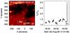 |
Fig. 1 a) A partial-frame SXR image observed by XRT at 01:03 UT on August 23. The two white boxes stand for the background region (BG) and the CBP. b) SXR light curve of the CBP. The light curve is calculated to be the total flux of the CBP normalized by the total flux of BG. Note the data gap in panel b). |
3. Results
3.1. Weak-flash phase
Figure 2 displays the evolution of CBP complex during the weak-flash phase. Initially, at 23:00:29 UT, it looked like a small diffuse loop with a horizontal size of 18″ located to the left of (−10″, 650″). A long arc-shaped bright loop, “Arc 1” hereafter, became evident, linking the right side of CBP to the northeast. Three minutes later at 23:03:09 UT, the small diffuse loop, which is labeled patch A (or PA) of the CBP became smaller and smaller, and another bright patch, which is labeled patch B (or PB) of the CBP became visible to the right of patch A near (−8″, 655″). At the same time, the bright loop “Arc 1” suddenly changed its connectivity at the western leg from the right side of the CBP to the left side. As seen from the attached movie, “Arc 1” detached from the solar surface during the transition and reconnected to the upper loop of CBP, forming a kinked loop structure resembling the number 7. At 23:14:21 UT, patch A reached the highest intensity and was apparently connected to patch B, while the remote or eastern leg of “Arc 1” was at its brightest as well. Afterwards, patch A of the CBP decayed rapidly, whereas patch B and the remote leg of “Arc 1” decayed much more slowly. At 00:40 UT on August 23, both patch A and “Arc 1” were invisible, and patch B was diffuse and faint.
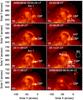 |
Fig. 2 a)−h) Eight snapshots of the SXR images during the weak-flash phase of the CBP. PA and PB stand for patch A and patch B of the CBP. “Arc 1” signifies the magnetic loop connecting the CBP with the remote leg (RL). BG denotes the background region used for the calculation of light curves in Fig. 3. The solid white line denoted with cut1 in panel d) is used for studying the transverse drift of “Arc 1”. An animation of this figure is available online. |
To illustrate the temporal relationship among the brightness of the two patches of CBP and the remote leg of large-scale loop “Arc 1”, the SXR light curves of the three parts are plotted in Fig. 3. The intensity for each part is the integral flux inside the corresponding boxes in Fig. 2, which is normalized by the total flux of a background region with the same area. As indicated by Fig. 3, patch A started to brighten at ~22:50 UT and reached its peak around 23:15 UT. The intensity of patch B increased from ~23:00 UT and peaked around 23:17 UT on August 22. The time delay between the peaks of the two patches was ~2 min. However, the highest intensity of the remote leg of “Arc 1” was nearly simultaneous with that of patch B, implying that the delay between them is shorter than the time cadence of the XRT observation (i.e., <32 s).
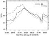 |
Fig. 3 SXR light curves of patch A (PA, dashed line), patch B (PB, solid line), and the remote leg of “Arc 1” (dotted line) during the weak-flash phase of the CBP. |
To better illustrate the transition of the connection of “Arc 1”, we extracted a cut across “Arc 1”, that is, cut1 in Fig. 2d. The time-slice diagram of cut1 is displayed in Fig. 4. It shows that the western leg of “Arc 1” drifted leftward at an apparent speed of ~16 km s-1 during the weak-flash phase, as indicated by the blue dashed line.
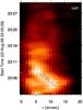 |
Fig. 4 Time-slice diagram of the SXR intensity along cut1 during the weak-flash phase. The dashed blue line stands for the leftward drift of “Arc 1”. The slope of the blue line represents the apparent drift speed (16 km s-1). |
3.2. Strong-flash phase
After 00:40 UT on August 23, patch B of the CBP was torpid for ~12 min before shining rapidly, with the brightness being stronger than ever. The evolution of CBP in the strong-flash phase is demonstrated in Fig. 5. At 00:59:45 UT, only patch B was identifiable, which looked like a small bright loop. Afterwards, its brightness increased drastically. When patch B flashed, a tiny region to the left of patch B became visible, which is indicated in Fig. 5c. Since the tiny bright region was located at the same site as patch A in the weak-flash phase mentioned in Sect. 3.1, we consider the tiny bright point as the recurrence of patch A of the CBP. Meanwhile, a brightening propagated rapidly along an arc-shaped loop from the top left of patch B to the remote site. Based on the same connectivity and cospatiality, we consider the large bright loop as the recurrence of “Arc 1”. At 01:05:05 UT, a jet-like structure emanated from the top-right of patch B and propagated along another bright loop “Arc 2” that was slightly shifted from “Arc 1” in Fig. 5d. At 01:06:41 UT, “Arc 1” suddenly changed its connectivity at the western leg from the left side of the CBP to the right side. At 01:09:21 UT, “Arc 1” was clearly rooted at the right side of patch B. At the same time, the left footpoint of patch B merged with patch A. After that, patch B disappeared rapidly, while patch A and “Arc 1” decayed slowly.
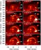 |
Fig. 5 a)−h) Eight snapshots of the SXR images during the strong-flash phase of the CBP. PA, PB, “Arc 1”, and RL have the same meanings as in Fig. 2. “Arc 2” signifies the magnetic loop adjacent to “Arc 1”. The solid white line denoted with cut2 in panel c) is used for studying the transverse drift of “Arc 1”. An animation of this figure is available online. |
As in the weak-flash phase, we investigated the temporal relationship between patches A and B. Because it is difficult to distinguish the two patches when the total intensity of patch B peaked, we selected two boxes in Fig. 5d that cover the main parts of patches A and B. The SXR flux inside the boxes was integrated separately and then normalized by the total SXR flux in the selected background area BG. The light curves of the two boxes representing patches A and B are plotted in Fig. 6. Patch B brightened first from ~00:58 UT and reached its peak at ~01:05 UT on August 23. The intensity of patch A increased from 01:00 UT and peaked around 01:07 UT on August 23. The time delay between the two patches, ~2 min, was very similar to that during the weak-flash phase.
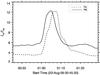 |
Fig. 6 SXR light curves of patch A (PA, dashed line) and patch B (PB, solid line) during the strong-flash phase of the CBP. The intensity of PA is multiplied by 1.8 for better comparison with PB. |
Like in Fig. 2d, we extracted another cut across “Arc 1”, that is, cut2 in Fig. 5c. The time-slice diagram of cut2 is displayed in Fig. 7. It reveals that the western leg of “Arc 1” drifted rightward at an apparent speed of ~4 km s-1 during the strong-flash phase.
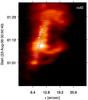 |
Fig. 7 Time-slice diagram of the SXR intensity along cut2 during the strong-flash phase. The dashed blue line stands for the rightward drift of “Arc 1”. The slope of the blue line represents the apparent drift speed (4 km s-1). |
4. Discussion and summary
Magnetic reconnection has been proposed to explain CBPs for a long time via different models whose differences lie in the magnetic configuration involved in the reconnection. Based on the light curves and potential fields of two CBPs, Zhang et al. (2012b) proposed that the embedded bipolar magnetic configuration might be responsible for the typical CBPs whose brightening consists of a weak gradual component and a quasi-periodic impulsive component, the latter was also called CBP flashes. According to the model, QSL reconnection or component reconnection accounts for the gradual component of brightening, whereas null-point reconnection accounts for the CBP flashes in nearly the same way as compact flares (Heyvaerts et al. 1977) or coronal jets (Shibata et al. 1992): a small bipolar magnetic loop (e.g., an emerging flux) reconnects with an overlying large loop or open fields. As mentioned by Moreno-Insertis et al. (2008), this type of reconnection is characterized by two chambers, a shrinking one containing the emerging magnetic loops and a growing one with loops produced by reconnection. They are located in the reconnection inflow and outflow regions. The two-chamber structure is discernible as patches A and B in Figs. 2 and 5. However, the role of each chamber in the two phases might be completely different.
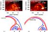 |
Fig. 8 Top panels: SXR images of the CBP event observed a) at 23:08 UT on August 22 and b) at 01:08 UT on August 23. “Arc 1”, “Arc 2”, PA, PB, and CBP have the same meanings as in Fig. 5. Bottom panels: cartoons that illustrate c) the weak and d) strong flash phases of the CBP event. The solid blue/red lines represent magnetic field lines in the inflow/outflow regions. The red crosses denote the X-point of the reconnection region. The black arrows point to the direction of mass motion. A and B stand for the magnetic field lines in the two patches of the CBP. |
Because the large-scale coronal loop drifted from the right to the left of the CBP, the magnetic configuration responsible for the weak-flash phase in Fig. 2 can be conceived and is illustrated in Fig. 8c: as the small bipolar loop A expands upward, it reconnects with the large-scale magnetic arc, producing bright loop B as the reconnected loop below the X-point. At the same time, the large-scale coronal loop, which is initially rooted at the right side of the two chambers as indicated by the long blue line, is now rooted at the left side of the two chambers after reconnection, as indicated by the red thatched field lines. For comparison, one snapshot of the observation is presented in Fig. 8a. All the components in the reconnection model, that is, loops A and B, and the thatched arc, resemble the observation very well. Therefore, the expanding bipolar loop in patch A corresponds to the reconnection inflow region during the weak-flash phase, and patch B corresponds to the reconnected loop in the outflow region.
During the strong-flash phase, patch B with a size of ~15″ brightened first as it expanded. Because the large-scale coronal loop drifted from left to the right of the CBP, the corresponding magnetic configuration can be conceived and is illustrated in Fig. 8d: as the bipolar loop B expands, it reconnects with the large-scale arc, producing bright patch A below the reconnection X-point. At the same time, the large-scale bright arc, which is rooted at the left side of the two chambers as indicated by the blue field line, is now rooted at the right side of the two chambers after reconnection, as indicated by the red thatched field lines. For comparison, one snapshot of the observation is shown in Fig. 8b. Therefore, in the strong-flash phase, patch B corresponds to the expanding bipolar field in the reconnection inflow region, and patch A corresponds to the reconnected loop in the outflow region, which is opposite to the case in the weak-flash phase.
It was proposed that fast-mode waves could modulate the null-point reconnection in a way that one pair of anti-parallel magnetic field lines serve as reconnection inflow and outflow successively (Craig & McClymont 1991; McLaughlin et al. 2009), which was called “oscillatory reconnection” and reproduced in the magnetohydrodynamic (MHD) numerical simulations of interaction between emerging flux and pre-existing magnetic fields in coronal holes (Murray et al. 2009; Archontis et al. 2010). Enhanced gas pressure in the reconnection outflow region becomes higher than that in the inflow region, forcing magnetic field lines in the two bounded outflow regions to reconnect reversely. As a result, an oscillatory reconnection and recurrent outflows (jets) are formed. In this paper, we report such a process in a CBP for the first time. To distinguish this phenomenon from the wave-modulated reconnection where the reconnection rate is modulated by waves but the inflow and the outflow do not reverse (Aschwanden et al. 1994; Chen & Priest 2006; Nakariakov et al. 2006), we call this phenomenon “reciprocatory reconnection”. As illustrated in Fig. 8, the successive brightenings of the CBP, with an interval of ~110 min that is close to twice the time interval of the recurrent CBP flashes (~120 min) studied by Zhang et al. (2012b), fit the reciprocatory reconnection very well. The difference between the simulations of Murray et al. (2009) and our observation is that the reconnection in Murray et al. (2009) is a pure dissipative process where the reconnection rate decreases with time. This is understandable since spontaneous magnetic reconnection is a dissipative process, the magnetic fields after reconnection contains less magnetic free energy. In our case, however, the highest reconnection rate appeared in the final reconnection stage (01:00−01:10 UT on August 23), implying that additional magnetic energy must be pumped into patch B after the weak-flash phase. A possible mechanism of energy pumping is the twisting motion of the photosphere. After reconnection in the first flash phase, the reconnected field (patch B in Fig. 8c) is close to potential field. However, during the following two hours, the everlasting convective motion in the solar photosphere may twist the bipolar loop in patch B, transferring Poynting flux into the coronal part. Such a twisting motion drives the bipolar loop in patch B to expand and then to reconnect with the overlying magnetic field. The reconnected field lines become the newly ignited patch A and the thatched large loop in Fig. 8d. The twisting motion-driven expansion and reconnection were numerically simulated by Pariat et al. (2009).
It has been revealed that a CBP is not just a simple bright point, it is often composed of a bundle of detailed substructures (Sheeley & Golub 1979; Dere 2008). Then the question is: what is the relation among the different parts of a CBP? Thanks to the high-resolution observations from Hinode/XRT, we are able to discover the substructures of a CBP and their evolution. After careful analysis, we found that the CBP consisted of two small bright loops, patches A and B. They were ignited alternately via reciprocatory reconnection. During the first flash phase, patch A corresponded to the reconnection inflow, whereas patch B corresponded to the reconnection outflow. However, 110 min later, patch B became the reconnection inflow, whereas patch A became the reconnection outflow during the second flash phase. The transverse drifts of the large-scale arc during the CBP flashes provide plausible evidence that the magnetic fields were rearranged. By combining the time delays between the peaks of the two patches with the opposite directions of drifts of the large-scale arc, we furthermore conclude that reciprocatory reconnection took place in the CBP. Assuming that the coronal Alfvén speed (vA) is ~1000 km s-1, the reconnection rate (vin/vA) in this CBP is roughly estimated to be around 0.01.
Generally speaking, when magnetic reconnection occurs, for example, in solar flares, the reconnection inflow region has the normal temperature, which is nearly the same as the background corona, whereas the reconnection outflow region is heated. The situation is different for CBPs, however. Taking the first flash phase, for example, its reconnection process can be well illustrated by Fig. 8c, where patch A corresponds to the reconnection inflow region and patch B corresponds to the reconnection outflow region. However, Fig. 2 indicates that patch A also brightened, and its brightness reached maximum even ~2 min before that of patch B. Based on the MHD simulations of Pariat et al. (2009) and the observational study of Zhang et al. (2012b), we conjecture that the brightening in the reconnection outflow (i.e., patch B) can be explained by the standard reconnection model for jets and CBPs (Shibata et al. 1992), whereas the brightening in the reconnection inflow (e.g., patch A) is due to QSL reconnection inside the twisting loop system itself as the convective photosphere drags the loop system, as simulated by Pariat et al. (2009). Recently, Moreno-Insertis & Galsgaard (2013) performed 3D numerical simulations of jet eruptions as a result of magnetic reconnection between an emerging flux rope and the pre-existing coronal magnetic field. In their numerical results no brightening can be seen in the reconnection inflow region, that is, in the emerging magnetic flux. The reason is probably that no twisting photospheric motion is exerted in the inflow region, whereas rotating motion is introduced in the bottom boundary conditions in Pariat et al. (2009).
In an embedded bipolar magnetic configuration, a spine links the magnetic null point to infinity (Fletcher et al. 2001; Pariat et al. 2010; Liu et al. 2011; Jiang et al. 2013) or to a remote place on the solar surface (Filippov 1999; Masson et al. 2009; Wang & Liu 2012; Sun et al. 2013). In the latter case, the released thermal energy and accelerated particles during reconnection would be transferred along the magnetic spine to heat the chromosphere and produce brightening at the other footpoint of spine, which has been discovered in flares (Biesecker & Thompson 2000; Wang et al. 2001; Moon et al. 2002; Brosius & Holman 2007; Su et al. 2013). Using the high-cadence Hinode/XRT observations, a similar phenomenon can be discovered in CBPs, as shown in Figs. 2 and 5 and in the online movies. The peak SXR intensities of the patch B in the CBP and the remote leg are nearly simultaneous. Considering the time cadence of the observation (32 s) and the distance between the remote brightening and the CBP (~35″), we can estimate the speed of energy transfer, which is >800 km s-1. Hence, the energy transfer is due to either thermal conduction or nonthermal particles.
In this paper, we performed a case study of the CBP event observed by Hinode/XRT on 2009 August 22−23. The CBP experienced two successive flashes, the first one was weak, the second one stronger. During the flashes, the appearances of a two-chamber structure and a drifting large-scale arc convincingly support the classical magnetic reconnection model where an expanding loop reconnects with the pre-existing magnetic fields. The large-scale arc drifted leftward (rightward) during the weak (strong) flash, with apparent speeds of 16 km s-1 and 4 km s-1. To the best of our knowledge, for the first time we discovered reciprocatory reconnection in a CBP event, that is, reconnected loops in the outflow region of the first reconnection process serve as the inflow of the second reconnection process. The time delay between the peak SXR intensities of the outflow and inflow regions was ~2 min during each phase. We also proposed a scenario to interpret the physical relation between the substructures within a CBP. Additional case studies are required to testify for or against the scenario using the high-cadence, high-resolution, and multiwavelength observations from the Solar Dynamic Observatory (SDO). MHD numerical simulations are also suitable to determine the mechanism of reciprocatory magnetic reconnection in CBPs.
Online material
Movie of Fig. 2 Access Supplementary Material
Movie of Fig. 5 Access Supplementary Material
Acknowledgments
The authors thank the referee for inspiring comments and suggestions. Q.M.Z. is grateful to Y. Guo and the Solar Physics group in Purple Mountain Observatory for valuable discussions. Hinode is a Japanese mission developed and launched by ISAS/JAXA, with NAOJ as domestic partner and NASA and STFC (UK) as international partners. This research is supported by the Chinese foundations NSFC (11303101, 11333009, 11173062, 11025314, 11373023, and 11221063) and by 973 program 2011CB811402.
References
- Archontis, V., & Hood, A. W. 2013, ApJ, 769, L21 [NASA ADS] [CrossRef] [Google Scholar]
- Archontis, V., Tsinganos, K., & Gontikakis, C. 2010, A&A, 512, L2 [NASA ADS] [CrossRef] [EDP Sciences] [Google Scholar]
- Aschwanden, M. J., Benz, A. O., & Montello, M. L. 1994, ApJ, 431, 432 [NASA ADS] [CrossRef] [Google Scholar]
- Aulanier, G., Golub, L., DeLuca, E. E., et al. 2007, Science, 318, 1588 [NASA ADS] [CrossRef] [Google Scholar]
- Biesecker, D. A., & Thompson, B. J. 2000, J. Atmospheric and Solar-Terrestrial Phys., 62, 1449 [Google Scholar]
- Brosius, J. W., & Holman, G. D. 2007, ApJ, 659, L73 [NASA ADS] [CrossRef] [Google Scholar]
- Chandrashekhar, K., Krishna Prasad, S., Banerjee, D., Ravindra, B., & Seaton, D. B. 2013, Sol. Phys., 286, 125 [NASA ADS] [CrossRef] [Google Scholar]
- Chen, P. F., & Priest, E. R. 2006, Sol. Phys., 238, 313 [NASA ADS] [CrossRef] [Google Scholar]
- Craig, I. J. D., & McClymont, A. N. 1991, ApJ, 371, L41 [NASA ADS] [CrossRef] [Google Scholar]
- Culhane, L., Harra, L. K., Baker, D., et al. 2007, PASJ, 59, 751 [Google Scholar]
- Dere, K. P. 2008, A&A, 491, 561 [NASA ADS] [CrossRef] [EDP Sciences] [Google Scholar]
- Filippov, B. 1999, Sol. Phys., 185, 297 [NASA ADS] [CrossRef] [Google Scholar]
- Filippov, B., Golub, L., & Koutchmy, S. 2009, Sol. Phys., 254, 259 [NASA ADS] [CrossRef] [Google Scholar]
- Fletcher, L., Metcalf, T. R., Alexander, D., Brown, D. S., & Ryder, L. A. 2001, ApJ, 554, 451 [NASA ADS] [CrossRef] [Google Scholar]
- Golub, L., Krieger, A. S., Harvey, J. W., & Vaiana, G. S. 1977, Sol. Phys., 53, 111 [NASA ADS] [CrossRef] [MathSciNet] [Google Scholar]
- Golub, L., Deluca, E., Austin, G., et al. 2007, Sol. Phys., 243, 63 [NASA ADS] [CrossRef] [Google Scholar]
- Guo, Y., Démoulin, P., Schmieder, B., et al. 2013, A&A, 555, A19 [NASA ADS] [CrossRef] [EDP Sciences] [Google Scholar]
- Habbal, S. R., & Withbroe, G. L. 1981, Sol. Phys., 69, 77 [NASA ADS] [CrossRef] [Google Scholar]
- Habbal, S. R., Withbroe, G. L., & Dowdy, Jr. J. F., 1990, ApJ, 352, 333 [Google Scholar]
- Handy, B. N., Acton, L. W., Kankelborg, C. C., et al. 1999, Sol. Phys., 187, 229 [NASA ADS] [CrossRef] [Google Scholar]
- Heyvaerts, J., Priest, E. R., & Rust, D. M. 1977, ApJ, 216, 123 [NASA ADS] [CrossRef] [Google Scholar]
- Huang, Z., Madjarska, M. S., Doyle, J. G., & Lamb, D. A. 2012, A&A, 548, A62 [NASA ADS] [CrossRef] [EDP Sciences] [Google Scholar]
- Jiang, C., Feng, X., Wu, S. T., & Hu, Q. 2013, ApJ, 771, L30 [NASA ADS] [CrossRef] [Google Scholar]
- Kariyappa, R., & Varghese, B. A. 2008, A&A, 485, 289 [NASA ADS] [CrossRef] [EDP Sciences] [Google Scholar]
- Kariyappa, R., Deluca, E. E., Saar, S. H., et al. 2011, A&A, 526, A78 [NASA ADS] [CrossRef] [EDP Sciences] [Google Scholar]
- Kosugi, T., Motsuzaki, K., Sakao, T., et al. 2007, Sol. Phys., 243, 3 [NASA ADS] [CrossRef] [Google Scholar]
- Kotoku, J., Kano, R., Tsuneta, S., et al. 2007, PASJ, 59, 735 [Google Scholar]
- Krieger, A. S., Vaiana, G. S., & van Speybroeck, L. P. 1971, Solar Magnetic Fields, 43, 397 [Google Scholar]
- Kwon, R.-Y., Chae, J., Davila, J. M., et al. 2012, ApJ, 757, 167 [Google Scholar]
- Lee, K.-S., Innes, D. E., Moon, Y.-J., et al. 2013, ApJ, 766, 1 [NASA ADS] [CrossRef] [Google Scholar]
- Liu, W., Berger, T. E., Title, A. M., Tarbell, T. D., & Low, B. C. 2011, ApJ, 728, 103 [NASA ADS] [CrossRef] [Google Scholar]
- Longcope, D. W. 1998, ApJ, 507, 433 [NASA ADS] [CrossRef] [Google Scholar]
- Madjarska, M. S., & Wiegelmann, T. 2009, A&A, 503, 991 [NASA ADS] [CrossRef] [EDP Sciences] [Google Scholar]
- Madjarska, M. S., Huang, Z., Doyle, J. G., & Subramanian, S. 2012, A&A, 545, A67 [NASA ADS] [CrossRef] [EDP Sciences] [Google Scholar]
- Mandrini, C. H., Démoulin, P., van Driel-Gesztelyi, L., et al. 1996, Sol. Phys., 168, 115 [NASA ADS] [CrossRef] [Google Scholar]
- Masson, S., Pariat, E., Aulanier, G., & Schrijver, C. J. 2009, ApJ, 700, 559 [NASA ADS] [CrossRef] [Google Scholar]
- McLaughlin, J. A., De Moortel, I., Hood, A. W., & Brady, C. S. 2009, A&A, 493, 227 [NASA ADS] [CrossRef] [EDP Sciences] [Google Scholar]
- Moon, Y.-J., Choe, G. S., Park, Y. D., et al. 2002, ApJ, 574, 434 [Google Scholar]
- Moore, R. L., Cirtain, J. W., Sterling, A. C., & Falconer, D. A. 2010, ApJ, 720, 757 [NASA ADS] [CrossRef] [Google Scholar]
- Moore, R. L., Sterling, A. C., Falconer, D. A., & Robe, D. 2013, ApJ, 769, 134 [NASA ADS] [CrossRef] [Google Scholar]
- Moreno-Insertis, F., & Galsgaard, K. 2013, ApJ, 771, 20 [NASA ADS] [CrossRef] [Google Scholar]
- Moreno-Insertis, F., Galsgaard, K., & Ugarte-Urra, I. 2008, ApJ, 673, L211 [Google Scholar]
- Murray, M. J., van Driel-Gesztelyi, L., & Baker, D. 2009, A&A, 494, 329 [NASA ADS] [CrossRef] [EDP Sciences] [Google Scholar]
- Nakariakov, V. M., Foullon, C., Verwichte, E., & Young, N. P. 2006, A&A, 452, 343 [NASA ADS] [CrossRef] [EDP Sciences] [Google Scholar]
- Pariat, E., Antiochos, S. K., & DeVore, C. R. 2009, ApJ, 691, 61 [NASA ADS] [CrossRef] [Google Scholar]
- Pariat, E., Antiochos, S. K., & DeVore, C. R. 2010, ApJ, 714, 1762 [NASA ADS] [CrossRef] [Google Scholar]
- Parnell, C. E., Priest, E. R., & Golub, L. 1994, Sol. Phys., 151, 57 [Google Scholar]
- Pérez-Suárez, D., Maclean, R. C., Doyle, J. G., & Madjarska, M. S. 2008, A&A, 492, 575 [NASA ADS] [CrossRef] [EDP Sciences] [Google Scholar]
- Pontin, D. I., Al-Hachami, A. K., & Galsgaard, K. 2011, A&A, 533, A78 [NASA ADS] [CrossRef] [EDP Sciences] [Google Scholar]
- Priest, E. R., Parnell, C. E., & Martin, S. F. 1994, ApJ, 427, 459 [NASA ADS] [CrossRef] [Google Scholar]
- Santos, J. C., Büchner, J., Madjarska, M. S., & Alves, M. V. 2008, A&A, 490, 345 [NASA ADS] [CrossRef] [EDP Sciences] [Google Scholar]
- Schmieder, B., Guo, Y., Moreno-Insertis, F., et al. 2013, A&A, 559, A1 [NASA ADS] [CrossRef] [EDP Sciences] [Google Scholar]
- Sheeley, Jr. N. R., & Golub, L. 1979, Sol. Phys., 63, 119 [NASA ADS] [CrossRef] [Google Scholar]
- Shibata, K., Ishido, Y., Acton, L. W., et al. 1992, PASJ, 44, L173 [NASA ADS] [CrossRef] [Google Scholar]
- Su, Y., Veronig, A. M., Holman, G. D., et al. 2013, Nat. Phys., 9, 489 [Google Scholar]
- Subramanian, S., Madjarska, M. S., & Doyle, J. G. 2010, A&A, 516, A50 [NASA ADS] [CrossRef] [EDP Sciences] [Google Scholar]
- Sun, X., Hoeksema, J. T., Liu, Y., et al. 2013, ApJ, 778, 139 [NASA ADS] [CrossRef] [Google Scholar]
- Tian, H., Xia, L.-D., & Li, S. 2008, A&A, 489, 741 [NASA ADS] [CrossRef] [EDP Sciences] [Google Scholar]
- Ugarte-Urra, I., Doyle, J. G., & Del Zanna, G. 2005, A&A, 435, 1169 [NASA ADS] [CrossRef] [EDP Sciences] [Google Scholar]
- van Driel-Gesztelyi, L., Schmieder, B., Cauzzi, G., et al. 1996, Sol. Phys., 163, 145 [NASA ADS] [CrossRef] [Google Scholar]
- Wang, H., & Liu, C. 2012, ApJ, 760, 101 [NASA ADS] [CrossRef] [Google Scholar]
- Wang, H., Chae, J., Yurchyshyn, V., et al. 2001, ApJ, 559, 1171 [NASA ADS] [CrossRef] [Google Scholar]
- Zhang, J., Kundu, M. R., & White, S. M. 2001, Sol. Phys., 198, 347 [NASA ADS] [CrossRef] [Google Scholar]
- Zhang, P., Fang, C., & Zhang, Q. 2012a, Science China Physics, Mechanics and Astronomy, 55, 907 [NASA ADS] [CrossRef] [Google Scholar]
- Zhang, Q. M., Chen, P. F., Guo, Y., Fang, C., & Ding, M. D. 2012b, ApJ, 746, 19 [NASA ADS] [CrossRef] [Google Scholar]
- Zhang, Q. M., & Ji, H. S. 2013, A&A, 557, L5 [NASA ADS] [CrossRef] [EDP Sciences] [Google Scholar]
- Zhang, Q. M., & Ji, H. S. 2014a, A&A, 561, A134 [NASA ADS] [CrossRef] [EDP Sciences] [Google Scholar]
- Zhang, Q. M., & Ji, H. S. 2014b, A&A, 567, A11 [NASA ADS] [CrossRef] [EDP Sciences] [Google Scholar]
All Figures
|
Fig. 1 a) A partial-frame SXR image observed by XRT at 01:03 UT on August 23. The two white boxes stand for the background region (BG) and the CBP. b) SXR light curve of the CBP. The light curve is calculated to be the total flux of the CBP normalized by the total flux of BG. Note the data gap in panel b). |
| In the text | |
|
Fig. 2 a)−h) Eight snapshots of the SXR images during the weak-flash phase of the CBP. PA and PB stand for patch A and patch B of the CBP. “Arc 1” signifies the magnetic loop connecting the CBP with the remote leg (RL). BG denotes the background region used for the calculation of light curves in Fig. 3. The solid white line denoted with cut1 in panel d) is used for studying the transverse drift of “Arc 1”. An animation of this figure is available online. |
| In the text | |
|
Fig. 3 SXR light curves of patch A (PA, dashed line), patch B (PB, solid line), and the remote leg of “Arc 1” (dotted line) during the weak-flash phase of the CBP. |
| In the text | |
|
Fig. 4 Time-slice diagram of the SXR intensity along cut1 during the weak-flash phase. The dashed blue line stands for the leftward drift of “Arc 1”. The slope of the blue line represents the apparent drift speed (16 km s-1). |
| In the text | |
|
Fig. 5 a)−h) Eight snapshots of the SXR images during the strong-flash phase of the CBP. PA, PB, “Arc 1”, and RL have the same meanings as in Fig. 2. “Arc 2” signifies the magnetic loop adjacent to “Arc 1”. The solid white line denoted with cut2 in panel c) is used for studying the transverse drift of “Arc 1”. An animation of this figure is available online. |
| In the text | |
|
Fig. 6 SXR light curves of patch A (PA, dashed line) and patch B (PB, solid line) during the strong-flash phase of the CBP. The intensity of PA is multiplied by 1.8 for better comparison with PB. |
| In the text | |
|
Fig. 7 Time-slice diagram of the SXR intensity along cut2 during the strong-flash phase. The dashed blue line stands for the rightward drift of “Arc 1”. The slope of the blue line represents the apparent drift speed (4 km s-1). |
| In the text | |
|
Fig. 8 Top panels: SXR images of the CBP event observed a) at 23:08 UT on August 22 and b) at 01:08 UT on August 23. “Arc 1”, “Arc 2”, PA, PB, and CBP have the same meanings as in Fig. 5. Bottom panels: cartoons that illustrate c) the weak and d) strong flash phases of the CBP event. The solid blue/red lines represent magnetic field lines in the inflow/outflow regions. The red crosses denote the X-point of the reconnection region. The black arrows point to the direction of mass motion. A and B stand for the magnetic field lines in the two patches of the CBP. |
| In the text | |
Current usage metrics show cumulative count of Article Views (full-text article views including HTML views, PDF and ePub downloads, according to the available data) and Abstracts Views on Vision4Press platform.
Data correspond to usage on the plateform after 2015. The current usage metrics is available 48-96 hours after online publication and is updated daily on week days.
Initial download of the metrics may take a while.