| Issue |
A&A
Volume 567, July 2014
|
|
|---|---|---|
| Article Number | A16 | |
| Number of page(s) | 22 | |
| Section | Interstellar and circumstellar matter | |
| DOI | https://doi.org/10.1051/0004-6361/201321113 | |
| Published online | 04 July 2014 | |
The structure of the thermally bistable and turbulent atomic gas in the local interstellar medium
1
Institut d’Astrophysique Spatiale, CNRS UMR 8617, Université Paris-Sud
11,
Bâtiment 121,
91405
Orsay,
France
e-mail:
This email address is being protected from spambots. You need JavaScript enabled to view it.
; This email address is being protected from spambots. You need JavaScript enabled to view it.
2
Canadian Institute for Theoretical Astrophysics, University of
Toronto, 60 St. George St.,
Toronto,
ON M5S 3H8,
Canada
3
Laboratoire de Radioastronomie, CNRS UMR 8112, École Normale Supérieure,
24 rue
Lhomond, 75231
Paris,
France
4
CEA, Maison de la Simulation, USR 3441, CEA-CNRS-INRIA- Univ.
Paris-Sud - Univ. de Versailles, 91191
Gif-sur-Yvette Cedex,
France
5
Institut für Astrophysik, Universität Göttingen,
Friedrich-Hund Platz
1, 37077
Göttingen,
Germany
Received:
15
January
2013
Accepted:
16
March
2014
Abstract
This paper is a numerical study of the condensation of the warm neutral medium (WNM) into cold neutral medium (CNM) structures under the effect of turbulence and thermal instability. It addresses the specific question of the CNM formation in the physical condition of the local interstellar medium (ISM). We use the properties of the H i deduced from observations and theoretical work to constrain the physical conditions in the WNM. Using low resolution simulations we explored the impact of the WNM initial density and properties of the turbulence (stirring in Fourier with a varying mix of solenoidal and compressive modes) on the cold gas formation to identify the parameter space that is compatible with the well established observational constraints of the H i in the local ISM. Two sets of initial conditions that match the observed quantity of CNM in mass were selected to produce high resolution simulations (10243) that allowed the properties of the produced dense structures to be studied in detail. We show that for typical values of the density, pressure and velocity dispersion of the WNM in the solar neighborhood, the turbulent motions of the H i cannot provoke the phase transition from WNM to CNM, regardless of their amplitude and their distribution in solenoidal and compressive modes. On the other hand, a quasi-isothermal increase in WNM density of a factor of 2 to 4 is enough to induce the phase transition, leading to the transition of about 40% of the gas to the cold phase within 1 Myr. This suggests that turbulence only induces the formation of the CNM when the WNM is pressured and put in a thermally unstable state. At the same time turbulence is regulating the formation of the CNM by preventing some of the WNM from moving toward the cold phase; indeed, tests performed on decaying simulations have shown that the fraction of CNM increases slowly in the decaying phase. In general, these results show that turbulence is playing a key role in the structure of the cold medium. The high resolution simulations show that the velocity field shows evidence of subsonic turbulence with a 2D power spectrum following a power law (P(k) ∝ k-2.4) close to Kolmogorov (P(k) ∝ k-2.67), while the density is highly contrasted with a significantly shallower 2D power spectrum (P(k) ∝ k-1.3), reminiscent of what is observed in the cold ISM. The cold structures denser than 5 cm-3 are characterized by power laws, M ∝ L2.25 and σ( | v | ) ∝ L0.41, that are similar to the ones observed in molecular clouds. The CNM structures are sub- or transonic, and their dynamic is tighly coupled to the WNM velocity field with a clump-to-clump velocity dispersion close to the velocity dispersion of the WNM. From this we conclude that suprathermal linewidth for CNM, inferred from 21 cm observations, might be the result of relative velocity between cold structures along the line of sight.
Key words: turbulence / instabilities / hydrodynamics / ISM: clouds / ISM: structure
© ESO, 2014
1. Introduction
Understanding the star formation process remains one of the main areas of research of modern astrophysics. It is directly linked to the way interstellar gas is organized and how dense and cold structures form. Turbulence plays a fundamental role here. It creates local increases in density that are amplified by gravity and that, in some cases, might lead to gravitational contraction. At the same time, the kinetic energy of turbulent motions needs to be dissipated in order for the gravitational collapse to happen. The overall star formation process is therefore directly linked to the way turbulence shapes the density structure of the ISM and how kinetic energy is transferred from large to small scales.
Where star formation occurs, molecular clouds exhibit suprathermal linewidths and strong contrast of density revealed by a lognormal histogram of column density (Vázquez-Semadeni & García 2001; Goodman et al. 2009; Federrath et al. 2010; Brunt 2010) and by power spectra of column density shallower (–2.5, Bensch et al. 2001) than predicted for subsonic or transonic turbulence (–3.66) and than what is observed in the diffuse H i (Miville-Deschênes et al. 2003a). For these reasons they are often modeled as isothermal and supersonic turbulent flows. On the other hand, because turbulence should dissipate in one dynamical time if it is not maintained on a large scale it is thought that star formation might occur within a dynamical (or free fall) time (Elmegreen 2000; Hartmann et al. 2001). In this scenario the gravitational collapse occurs during the cloud formation. Therefore, the initial conditions of the star formation process depend strongly on the structure of the cold clouds in the atomic phase (H i).
Most of the mass of the Galactic interstellar medium (ISM) is H i and there is
clear observational evidence that it is thermally bistable (Dickey et al. 2003); it consists of two thermally stable states at significantly
different temperatures (the cold neutral medium – CNM – and the warm neutral medium – WNM).
This is a natural result of the density and temperature dependence of the cooling processes
in play in the diffuse ISM. Like molecular clouds, the structure of the H i is
highly complex with strong density contrasts (the CNM fills only about 1% of the volume but
has a density 100 times higher than the WNM), but here the combination of turbulence and
thermal instability (TI; Field 1965, 1969) is the
main driver of the structure. It is important to note that the nature of the density
fluctuations in an isothermal and supersonic flow is conceptually different than in a
thermally bistable fluid. An isothermal turbulent flow with supersonic velocity fluctuations
will naturally develop strong density fluctuations ( , Vázquez-Semadeni 2012). In such a flow the density
fluctuations are transient, associated with the compression and depression of the turbulent
motions. In a two-phase medium, once a high density structure is created by a local
compression it remains at high density even when the gas re-expand because it is in pressure
equilibrium with the inter-cloud medium. A two-phase medium will therefore produce
long-lived high density structures contrary to supersonic flows in which the fluctuations
appear and disappear on dynamical timescales. Therefore the thermally bistable H i
offers a natural way of producing highly structured initial conditions for the star
formation in molecular clouds.
, Vázquez-Semadeni 2012). In such a flow the density
fluctuations are transient, associated with the compression and depression of the turbulent
motions. In a two-phase medium, once a high density structure is created by a local
compression it remains at high density even when the gas re-expand because it is in pressure
equilibrium with the inter-cloud medium. A two-phase medium will therefore produce
long-lived high density structures contrary to supersonic flows in which the fluctuations
appear and disappear on dynamical timescales. Therefore the thermally bistable H i
offers a natural way of producing highly structured initial conditions for the star
formation in molecular clouds.
Because of the complex dynamical processes involved, dedicated numerical simulations are useful to develop insights on the exact scenario that leads to the formation of cold structures in the H i. Several studies based on numerical simulations have explored the thermally bistable physics of the H i since the early one-dimensional work of Hennebelle & Pérault (1999) who showed the effect of compression in a WNM converging flow on the triggering of the phase transition and the production of CNM structures. Similarly Koyama & Inutsuka (2000, 2002) studied the impact of the propagation of a shock wave into WNM. They showed how CNM structures form in the post-shock region through the thermal instability which operates faster than the duration of the shock (galactic spiral shock or supernova). In both cases the resulting density contrast between the CNM and WNM is ~100. To obtain a similar contrast in isothermal supersonic turbulence, Mach numbers of the order of 10 are required. These studies have been extended to two and three dimensions simulations of thermally bistable flows with turbulence induced by a converging flow (Audit & Hennebelle 2005; Hennebelle & Audit 2007; Hennebelle et al. 2007; Audit & Hennebelle 2010; Heitsch et al. 2005, 2006), by the magneto-rotational instability (Piontek & Ostriker 2004, 2005, 2007; Piontek et al. 2009) or by a driving in Fourier space (Gazol et al. 2005; Gazol & Kim 2010; Seifried et al. 2011).
It was established that compression of the WNM in transonic converging flows triggers the thermal instability; the increase in density can be such that the gas cools rapidly to temperatures of a few tens of degrees. The cold gas then fragments into clumps, in particular through the Kelvin-Helmholtz instability (Heitsch et al. 2006). The thermal pressure of the cold gas is in approximate equilibrium with the sum of the ram and thermal pressure of the surrounding warm gas. Once pushed at high enough densities, the cold structures can have densities and temperatures close to values typical of molecular clouds (Vázquez-Semadeni et al. 2006; Banerjee et al. 2009).
In general, previous works showed that the efficiency of the formation of the CNM depends directly on the nature and amplitude of the injected energy. One question we wanted to explore in this study is related to the driving of the compression. Most studies have explored the case of converging flows where the increase of the WNM density needed to trigger the thermal instability is obtained by a sustained ram pressure. The origin of such large scale convergent flows is unclear so here we want to see if compression in turbulent motions alone, driven on large scales, could lead to the production of cold gas. More precisely, we wanted to see if turbulent motions, at the level they are observed in the WNM, can induce the phase transition and if not, what are the required physical conditions of the WNM to trigger the formation of cold structures. To do so, like Gazol et al. (2005), Gazol & Kim (2010), Seifried et al. (2011), we used turbulent forcing in Fourier space. In addition, similarly to the study of Federrath et al. (2010) based on isothermal simulations of molecular clouds, we wanted to study the impact of compressive and solenoidal modes in the injected turbulent field.
In this paper we present a parameter study of WNM initial density and turbulent forcing properties on the formation of the CNM in forced turbulence and thermally bistable flows. In a similar study, Seifried et al. (2011) chose initial densities (1 to 3 cm-3) that are in the thermally unstable regime, to expect the production of a two-phase medium. Our intent is to expand the parameter space to identify the dynamical conditions that lead to the formation of the cold phase. In addition, one fundamental aspect of the current study is that we guide our parameter search based on all available observational constraints of the local ISM. We present 90 simulations performed on a 1283 grid that allowed us to identify more precisely the physical conditions that favor the formation of cold structures while reproducing in detail the observed properties of the H i in the local ISM. For two specific cases that match the observations we performed two 10243 simulations in order to study in greater details the properties of the H i: temperature, pressure and density histograms, power spectra, and mass-size and velocity dispersion-size relations of the cold structures.
The paper is organized as follow. HERACLES, the numerical code used in this study is briefly presented in Sect. 2. The observational constrains used to lead the parameter study are detailed in Sect. 3. The methodology is presented in Sect. 4. The results of the parametric study and of the high resolution simulations are presented and discussed in Sects. 5 and 6 respectively. The main conclusions of the study are given in Sect. 7.
2. Numerical methods
Despite their great importance in the ISM, we won’t consider magnetic field or gravity in this study to focus on the impact of vortical and compressive turbulence motions on the formation of CNM. All the following simulations are thus hydrodynamical. We performed our simulations with HERACLES (González et al. 2007). The numerical methods are similar to those described in Audit & Hennebelle (2005).
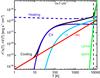 |
Fig. 1 Heating and cooling processes implemented in HERACLES based on Wolfire et al. (1995, 2003). We represent the respective rates of energy-densities gains and losses versus the temperature at the fixed density n = 1 cm-3, typical of the WNM. The total cooling (black solid curve) is decomposed in its different components: CII (dark blue), OI (light blue), recombination on interstellar grains (red), Lyman α (green). The dashed blue line is the heating dominated by the photo-electric effect on small dust grains. We considered a spatially uniform radiation field with the spectrum and intensity of the Habing field (G0/ 1.7 where G0 is the Draine flux) (Habing 1968; Draine 1978). |
2.1. Euler equations and Godunov scheme
The Euler equations for a radiatively cooling gas are the classical equations of
hydrodynamics used for flows at high Reynolds number, which is the case in the ISM:
![Mathematical equation: \begin{eqnarray} && \partial_t\rho + \nabla\cdot[\rho {\vec u} ] = 0, \\ && \partial_t[\rho {\vec u}] + \nabla\cdot[\rho {\vec u}\otimes {\vec u} +P] = \rho {\vec f}, \\ && \partial_tE + \nabla\cdot[{\vec u}(E+P)] = \rho {\vec f}\cdot {\vec u}-\mathcal{L}(\rho,T) \end{eqnarray}](/articles/aa/full_html/2014/07/aa21113-13/aa21113-13-eq16.png) where
ρ is the
mass density, u the velocity, P the pressure and
E the total
energy. The atomic gas is considered perfect and ideal with an adiabatic index
γ = 5 /
3 and a mean atomic weight μ = 1.4 mH
(mH is the mass of the proton). The weight
μ takes the
cosmic abundance of other elements into account: helium and metals, and so the mass
density is ρ =
μ × n.
where
ρ is the
mass density, u the velocity, P the pressure and
E the total
energy. The atomic gas is considered perfect and ideal with an adiabatic index
γ = 5 /
3 and a mean atomic weight μ = 1.4 mH
(mH is the mass of the proton). The weight
μ takes the
cosmic abundance of other elements into account: helium and metals, and so the mass
density is ρ =
μ × n.
The net cooling function is defined as ℒ = n2Λ − nΓ (expressed in erg cm-3 s-1), where Λ and Γ are respectively the cooling and heating terms based on the prescription of Wolfire et al. (1995, 2003). They include the most relevant processes in the diffuse medium for our range of temperature [10 K, 104 K] and are plotted and described in Fig. 1 (for more details, see Audit & Hennebelle 2005). The equations solver in HERACLES is a second order Godunov scheme (see Audit & Hennebelle 2010) for the conservative part. It is a MHD solver of type MUSCL-Handcook (Londrillo & Del Zanna 2000; Fromang et al. 2006). The cooling is applied after the solver (see Audit & Hennebelle 2005).
2.2. Turbulence forcing
An external field f, applied in Fourier space, is added to generate large scale turbulent motions. It has the dimension of an acceleration. A study of a driving consisting of a true force compared to a driving consisting of an acceleration has been performed by Wagner et al. (2012). They demonstrated that modeling the force density instead of the acceleration at low wavenumbers directly couples the external energy injection to all scales of the system, as the density field has Fourier modes over the whole range of wavenumbers.
The magnitude of the applied acceleration is  where
vS represents the amplitude given to the
field1 and LS =
Lbox/k0
is the characteristic integration scale with k0 = 2 the characteristic wave number of
the stirring. The auto-correlation time of the process is given by τS =
(LS/FS)1/2 =
LS/vS.
The stirring is applied on large scales, and thus to the small wave numbers:
0 < |
k | <
2k0.
where
vS represents the amplitude given to the
field1 and LS =
Lbox/k0
is the characteristic integration scale with k0 = 2 the characteristic wave number of
the stirring. The auto-correlation time of the process is given by τS =
(LS/FS)1/2 =
LS/vS.
The stirring is applied on large scales, and thus to the small wave numbers:
0 < |
k | <
2k0.
The modes of the turbulent forcing are computed with the stochastic process of
Ornstein-Uhlenbeck (Eswaran & Pope 1988;
Schmidt et al. 2006). The method is similar to
Schmidt et al. (2009) and Federrath et al. (2010). A Helmholtz decomposition is applied to the
random field to project it on its compressive and solenoidal components. The projection
operator is defined as 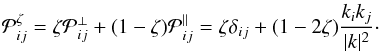 (4)Choosing
a spectral weight ζ =
1 creates a divergence free field, i.e. purely solenoidal. Taking
ζ <
1 generates dilatational components which compress or rarify the gas.
Finally, ζ =
0 creates a rotation-free field, i.e. purely compressive. In a natural
state for which the energy is naturally distributed between the compressive and solenoidal
modes (2:1 mixing), ζ takes the value of 0.5. In this case, the Helmholtz
operator is proportional to the identity operator and the projection does not alter the
energy repartition between the different modes.
(4)Choosing
a spectral weight ζ =
1 creates a divergence free field, i.e. purely solenoidal. Taking
ζ <
1 generates dilatational components which compress or rarify the gas.
Finally, ζ =
0 creates a rotation-free field, i.e. purely compressive. In a natural
state for which the energy is naturally distributed between the compressive and solenoidal
modes (2:1 mixing), ζ takes the value of 0.5. In this case, the Helmholtz
operator is proportional to the identity operator and the projection does not alter the
energy repartition between the different modes.
3. Observational constraints
The simulations presented in this study are dedicated to the formation of CNM structures out of pure WNM gas. In this section we present global properties of the Galactic H i as deduced from the observations. These properties guided us in the choice of the initial conditions of the simulations and on the qualification of the results obtained.
3.1. Pressure and thermal bistability of the H I
Because of the density and temperature dependence of the heating and cooling processes in the diffuse ISM (see Fig. 1) it has been shown early on by Field (1965), Field et al. (1969) and updated by Wolfire et al. (1995, 2003) that there is a range of pressure where the neutral atomic gas can be in two thermally stable phases in pressure equilibrium. This is often displayed in diagrams like the ones shown in Fig. 2 where the solid curves in the two panels indicate the locus of thermal equilibrium in the P − n and T − n parameter spaces.
The thermal stability is not preserved everywhere along these curve but only where dP/dn > 0. The two dash-dotted vertical lines mark the boundaries in density where the H i is thermally unstable. Any perturbation of the gas sitting on the equilibrium curve in the thermally unstable range would move toward the cold or warm branches. From Fig. 2 one can appreciate the steepness of the equilibrium curve in T − n space, highlighting the great difference in temperature and density of the two stable phases of the H i.
It is important to point out that the bistability of the H i is only present in a given range of pressure, determined by the maximum density of the warm branch (n ~ 0.8 cm-3) and the minimum density of the cold branch (n ~ 7 cm-3). For P < 1000 Kcm-3 there is no CNM and for P> 6000 Kcm-3 all the H i is cold.
On the top panel of Fig. 2 the dashed curve gives the average pressure observed in the local ISM. According to Jenkins & Tripp (2011) the pressure of the cold phase follows a log-normal distribution with an average of log 10(P/k) equals to 3.58 dex and minimum and maximum values (at the 99% level) equal to 3.04 and 4.11 dex (dotted lines). The minimum CNM pressure reported by Jenkins & Tripp (2011) corresponds exactly to the minimum CNM pressure (3.06 dex) allowed by the thermal instability (see Fig. 2) as predicted by the modeling of the heating and cooling processes of Wolfire et al. (1995, 2003). The maximum pressure reported by Jenkins & Tripp (2011) is significantly higher than the maximum pressure allowed for the thermally stable WNM (3.74 dex). At such high pressure the gas can only be thermally stable in the cold phase.
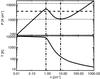 |
Fig. 2 Equilibrium temperature and pressure as a function of density. These equilibrium curves were computed equating the heating and cooling processes described in Wolfire et al. (1995, 2003). The dashed line corresponds to the average pressure of the cold diffuse ISM measured by Jenkins & Tripp (2011). The dotted lines show the maximum and minimum pressures that include 99% of the data of Jenkins & Tripp (2011). The dash-dotted lines show the density range of the thermally unstable phase. |
3.2. WNM density and temperature
Here we want to estimate what is the true density (as opposed to space-averaged) and temperature of the WNM in the local ISM. Typical numbers cited are n ~ 0.2−0.5 cm-3 and T ~ 6000 − 104 K (Ferrière 2001), but, as emphasized by Kalberla & Dedes (2008), the density of the WNM varies greatly with galacto-centric radius and galactic height z. It is also subject to local variations due to star formation activity (e.g. supernovae, Joung et al. 2009) and between the arm and inter-arm regions.
According to Dickey & Lockman (1990, see also Celnik et al. 1979; Malhotra 1995; Kalberla et al. 2007), the distribution of the H i density with z close to the Sun can be decomposed in a narrow Gaussian of HWHM = 106 pc, a broader Gaussian of HWHM = 265 pc and an exponential with a scale height of 403 pc. Generally the narrow Gaussian is attributed to the CNM and the sum of the two others to the WNM. In this scheme, and still following Dickey & Lockman (1990), the space-average density of the CNM and WNM at z = 0 are 0.395 cm-3 and 0.172 cm-3 respectively. These values are weighted by the volume filling factor φ and thus correspond to nφ, where n is the true volume density. The filling factor of the WNM is difficult to estimate; according to Kalberla & Kerp (2009)φ ~ 40% which implies a true density of nWNM = 0.43 cm-3.
This value is close to the one that can be derived based on the knowledge of the heating and cooling processes. For the average pressure of P = 3980 Kcm-3 found by Jenkins & Tripp (2011), using the heating and cooling curves of Wolfire et al. (1995, 2003) and assuming a spatially uniform radiation field with the spectrum and intensity of the Habing field (G0/ 1.7 where G0 is the Draine flux – Habing 1968; Draine 1978), the equilibrium density and temperature of the WNM are nwnm = 0.5 cm-3 and Twnm = 7960 K.
Figure 3 shows how n, T and P vary with z assuming a scale height of HWHM = 265 pc for the WNM disk at R = R⊙ (Dickey & Lockman 1990; Malhotra 1995; Kalberla et al. 2007). Assuming a true volume density nWNM = 0.5 cm-3 at z = 0, the corresponding temperature profile T(z) of the WNM can be estimated using the thermal equilibrium curve based on the heating and cooling processes described in Wolfire et al. (1995, 2003). It shows that the variations with z of the WNM properties due to the hydrostatic equilibrium become important only on scales larger than 100 pc.
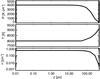 |
Fig. 3 Vertical distribution of the WNM density, temperature and pressure in the disk of the Milky Way, at the Sun galacto-centric radius. The density profile assumes n(z = 0) = 0.5 cm-3, in accordance with the mean pressure of Jenkins & Tripp (2011) and the heating and cooling processes described in Wolfire et al. (2003). The scale height of the WNM is the value of Dickey & Lockman (1990): HWHM = 265 pc. The temperature is computed at each position z assuming thermal equilibrium at density n(z). The pressure is simply P/k = nT. |
3.3. WNM turbulent velocity dispersion and Mach number
Apart from its density and temperature, the other relevant parameter for this study is the level of turbulence in the WNM, or equivalently its Mach number. The direct estimate of the Mach number of the WNM is difficult due to its temperature that cannot be easily measured. The traditional method to estimate the H i temperature is based on a comparison of 21 cm absorption and emission measurements. Due to its low opacity, the warm phase produces almost undetectable absorption once observed in front of a strong radio-continuum source. Only a few detections were reported so far (e.g. Carilli et al. 1998; Kanekar et al. 2003; Begum et al. 2010), with deduced temperatures closer to the thermally unstable regime (T ~ 500−6000 K) than to what is expected for the WNM (T ~ 8000 K).
Nevertheless there is indirect evidence that the warm ISM is subsonic. Recent findings on the warm ionized medium (WIM) by Gaensler et al. (2011) confirmed the work of Armstrong et al. (1995) and Redfield & Linsky (2004) that showed that the WIM has the properties of a low Mach number and incompressible turbulent flow. Regarding the WNM, an indication of its low Mach number comes from the smoothness of the 21 cm profiles. Haud & Kalberla (2007) found that the simplest 21 cm spectra of the LAB data (Kalberla et al. 2005) at high Galactic latitudes are well modeled by a single Gaussian of σtot = 10.2 ± 0.3 km s-1. Here we assume this value to be representative of the WNM total velocity dispersion in the solar neighborhood.
The WNM velocity dispersion is the quadratic sum of the thermal (σtherm) and
turbulent (σturb) contribution to the gas motions,
integrated along the line of sight. Considering the specific line of sight at the Galactic
pole, the thermal contribution to the linewidth of the WNM is an integral over Galactic
height z:
![Mathematical equation: \begin{eqnarray} \label{eq:sigma_therm} \sigma_{\mathrm{therm}} = \left[ \frac{k}{m}\frac{\int_0^L n(z) T(z) {\rm d}z}{\int_0^Ln(z){\rm d}z} \right]^{1/2} \end{eqnarray}](/articles/aa/full_html/2014/07/aa21113-13/aa21113-13-eq80.png) (5)where
n(z) is assumed to be a Gaussian
with HWHM =
265 pc (Dickey & Lockman
1990). Using the corresponding T(z) shown in Fig. 3, integrating Eq. (5) gives σtherm = 8.3 km s-1, a value essentially identical
to the thermal width of an isothermal 8000 K gas (σtherm =
8.1 km s-1) which illustrates that the WNM temperature does not
vary significantly with Galactic height. Assuming σtot =
10.2 km s-1 (Haud & Kalberla
2007), the contribution of turbulent motions to the observed linewidth is
σturb =
5.9 km s-1. That σturb < σtherm
is another indication that thermal motions dominates over turbulent motions on any scale
in the solar neighborhood.
(5)where
n(z) is assumed to be a Gaussian
with HWHM =
265 pc (Dickey & Lockman
1990). Using the corresponding T(z) shown in Fig. 3, integrating Eq. (5) gives σtherm = 8.3 km s-1, a value essentially identical
to the thermal width of an isothermal 8000 K gas (σtherm =
8.1 km s-1) which illustrates that the WNM temperature does not
vary significantly with Galactic height. Assuming σtot =
10.2 km s-1 (Haud & Kalberla
2007), the contribution of turbulent motions to the observed linewidth is
σturb =
5.9 km s-1. That σturb < σtherm
is another indication that thermal motions dominates over turbulent motions on any scale
in the solar neighborhood.
Due to the nature of the turbulent cascade, the turbulent velocity dispersion increases with scale like σturb = σ(1)lq, where q ~ 1/3 for subsonic turbulence and, following the notation of Wolfire et al. (2003), σ(1) is the velocity dispersion (in km s-1) on a scale of 1 pc and l is the scale (in pc). Assuming that the turbulent contribution to the observed linewidth is representative of motions on the scale of the H i scale height at the Sun location (l = hz = 265 pc), one obtains σ(1) = 0.92 km s-1. This calculation is similar to the one of Wolfire et al. (2003) who estimated σ(1) = 1.4 km s-1 for the WNM. That we obtain a significantly lower value can be attributed mostly to our having taken the thermal contribution to the linewidth into account.
3.4. CNM mass fraction and volume filling factor
One important quantity we want to reproduce in the simulations is the amount of mass in the cold phase. The CNM mass fraction was estimated to 40% by Heiles & Troland (2003) by comparing 21 cm absorption and emission measurements on 79 random lines-of-sights. This is also compatible with the decomposition of the H i density distribution with z of Dickey & Lockman (1990); their narrow component (h = 106 pc) that can be associated to the CNM contributes to 44% of the total H i surface density of the disk. Because the scale height of the CNM is less than for the WNM, the CNM mass fraction varies with z. The CNM contributes to 60% of the H i mass for z < 200 pc.
Like for the WNM one can compute the expected CNM volume density based on the heating and cooling processes (Wolfire et al. 1995, 2003). For the average pressure of Jenkins & Tripp (2011, P = 3980 Kcm-3) the equilibrium density and temperature are ncnm = 111 cm-3, Tcnm = 35.9 K. Following Dickey & Lockman (1990), the space-average density of the CNM is ~0.4 cm-3 at z = 0, which implies a volume filling factor of the cold phase lower than 1%.
4. Methodology
Based on the observational constraints described in the previous section, we conclude that the WNM in the solar neighborhood has a mean temperature T ~ 8000 K, a mean density of n ~ 0.2−0.5 cm-3 and subsonic turbulent motions following σturb = 0.92 (l/1pc)1/3 (km s-1). The first step of this study is to evaluate what are the plausible dynamical conditions that lead to the formation of CNM gas, of the order of 40% in mass, from WNM gas with such physical properties. We explored those conditions with 90 simulations at low resolution (1283 cells). In a second step, two sets of initial conditions that match the H i observations are used to produce high resolution simulations (10243) and study in more details the properties of the CNM structures.
In this section we first described the characteristic scales involved in the simulations, then we validate the use of 1283 simulations for the exploration of the parameters space by comparing with higher resolution (2563 and 5123) simulations.
4.1. Characteristic scales
4.1.1. Dynamical time and cooling scale of the WNM
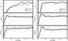 |
Fig. 4 Time evolution of the CNM mass fraction fCNM, the mean velocity dispersion σturb and the mean Mach number ℳobs for simulations with the following initial conditions: on the left n0 = 1cm-3, ζ = 0.2, vS = 12.5 km s-1, on the right n0 = 2 cm-3, ζ = 0.5, vS = 7.5 km s-1, and different resolutions: 5123 (solid black line), 2563 (dotted blue line) and 1283 cells (dashed green line). |
If, during the perturbation of an initial WNM cloud, the cooling processes act slower
than the compressive ones, the gas will tend to return to its initial state of
temperature and density by decompression. The WNM-CNM transition becomes possible when
the radiative time is lower than the dynamical time (Hennebelle & Pérault 1999), allowing the condensed gas to keep its
higher density even during the decompression:  (6)The
dynamical time is defined as the time needed by an atom to cross the cloud (of size
d) at the
sound speed velocity cS:
(6)The
dynamical time is defined as the time needed by an atom to cross the cloud (of size
d) at the
sound speed velocity cS:
 (7)The
radiative time is the characteristic time needed by the medium to cool. It is the ratio
of the energy (U) to the energy transfer (ϵ) applied to the medium:
(7)The
radiative time is the characteristic time needed by the medium to cool. It is the ratio
of the energy (U) to the energy transfer (ϵ) applied to the medium:
 (8)From
these equations we can calculate the critical size above which the WNM will be unstable
and will condense into the unstable regime or CNM structures. We consider typical
conditions of the WNM (T =
8000 K and n = 0.5 cm-3) and a static medium,
assuming that the energy is fully thermal. Using Eq. (6) and the heat capacity per mass unity CV =
kB/mH(γ − 1):
(8)From
these equations we can calculate the critical size above which the WNM will be unstable
and will condense into the unstable regime or CNM structures. We consider typical
conditions of the WNM (T =
8000 K and n = 0.5 cm-3) and a static medium,
assuming that the energy is fully thermal. Using Eq. (6) and the heat capacity per mass unity CV =
kB/mH(γ − 1): 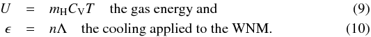 The
cooling time thus becomes:
The
cooling time thus becomes: 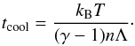 (11)Considering
the main cooling processes of the diffuse H i described in Sect. 3.1 to evaluate Λ, and using
(11)Considering
the main cooling processes of the diffuse H i described in Sect. 3.1 to evaluate Λ, and using
 ,
one obtains the following WNM cooling scale:
,
one obtains the following WNM cooling scale:
 (12)Therefore,
for the thermal instability to develop, the scale of the dynamically perturbed WNM must
be greater than λcool ~ 22 pc. Similarly, a
perturbation of size lower than λcool do not efficiently trigger the
phase transition.
(12)Therefore,
for the thermal instability to develop, the scale of the dynamically perturbed WNM must
be greater than λcool ~ 22 pc. Similarly, a
perturbation of size lower than λcool do not efficiently trigger the
phase transition.
4.1.2. Sizes of the simulations
To study the WNM-CNM transition it is important to evaluate the scales of cold structures, in order to adjust the numerical resolution. As illustrated by the 2D simulations of Hennebelle et al. (2007) and the 3D simulations of Audit & Hennebelle (2010), the size of the CNM clumps are distributed in the range 10-3−0.5 pc. Moreover, the Field length λF (Field 1965; Begelman & McKee 1990), which gives the typical scale of the thermal front between the WNM and the CNM, as well as the shock front of CNM structures, are both of the order of 10-3 pc. Therefore, in principle simulations of the thermally bistable H i would require a resolution of the order of 10-3 pc. Nevertheless, as suggested by Hennebelle & Audit (2007) and as we will show in the next section, the most important scale to resolve in simulations of thermally bistable and turbulent H i is the “sound crossing scale” (i.e., the sound speed times the cooling time). As described in the previous section, this scale is ~22 pc for typical values of the WNM density, providing a minimum size for the simulation box. We chose to assure the phase transition with a box size equal to 40 pc. In the following we use box sizes of 1283 pixels and 10243 pixels, corresponding respectively to resolution of 0.3 and 0.04 pc.
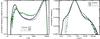 |
Fig. 5 Histograms of temperature weighted by density (left) and density (right). Curves shown are for simulations with initial conditions of n0 = 1 cm-3, ζ = 0.2, vS = 12.5 km s-1, and different resolutions: 5123 (solid black line), 2563 (dotted blue line) and 1283 cells (dashed green line). All histograms were computed at t = 40 Myr. |
4.2. Effect of resolution
In Sect. 5 we present a parametric study based on
1283 pixels
simulations. Even though we barely resolve the typical scale of CNM structures with those
simulations, we will demonstrate using higher resolution simulations that this set up can
be used to explore efficiently the parameter space for the formation of the CNM. Figure
4 shows the evolution over time of the CNM mass
fraction, the dispersion of the line of sight turbulent velocity σturb and the
observational Mach number for two representative simulations ([n0 = 1
cm-3,
ζ = 0.2,
vS =
12.5 km s-1] and [n0 = 2 cm-3, ζ = 0.5, vS = 7.5
km s-1]) done on
1283,
2563 and
5123 grids. We
calculate the cold mass fraction fCNM as the sum of the mass in pixels
where T < 200 K, over the total
mass in the box. The turbulent velocity dispersion is computed the following way (see
Miville-Deschênes & Martin 2007, Eq.
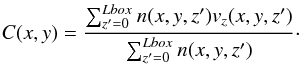
(8)): 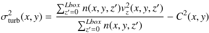 (13)where
C(x,y) is the velocity centroid at
position (x,y):
(13)where
C(x,y) is the velocity centroid at
position (x,y):
 (14)In
numerical simulations, the Mach number is often computed as the ratio of the velocity and
the sound speed on each cell:
(14)In
numerical simulations, the Mach number is often computed as the ratio of the velocity and
the sound speed on each cell: 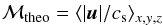 (15)where
 .
Because this parameter cannot be directly deduced from observations we consider an
expression for the Mach number calculated from integrated quantities along the line of
sight, the turbulent velocity dispersion and the thermal velocity dispersion:
.
Because this parameter cannot be directly deduced from observations we consider an
expression for the Mach number calculated from integrated quantities along the line of
sight, the turbulent velocity dispersion and the thermal velocity dispersion:
 (16)where
the thermal velocity dispersion is defined as
(16)where
the thermal velocity dispersion is defined as  (17)Obviously
the total2 velocity dispersion is simply
(17)Obviously
the total2 velocity dispersion is simply
 (18)All
quantities shown in Fig. 4 are averaged over the box
at different time steps. For all resolution, the mean values of σturb and
ℳobs are in the
same range, and their variations are of the same order. These two quantities are thus
statistically well represented even in small resolution simulations.
(18)All
quantities shown in Fig. 4 are averaged over the box
at different time steps. For all resolution, the mean values of σturb and
ℳobs are in the
same range, and their variations are of the same order. These two quantities are thus
statistically well represented even in small resolution simulations.
The evolution with time of fCNM (Fig. 4) as well as the histograms of temperature and density (Fig. 5) indicate that the fraction of the mass in the cold gas depends on the numerical resolution. Higher resolution runs lead to a slightly higher amount of cold gas. The cold peak of the temperature histogram (Fig. 5) is lower in the 1283 and 2563 cases. The time evolution of fCNM increases more slowly for the smallest resolution run. Nevertheless, the differences in the mass fraction of gas with T < 200 K after 40 Myr remain small for the different resolutions (see Fig. 4). We verified that these results are independant of the initial conditions.
From this analysis, and like Seifried et al. (2011), we conclude that the resolution does not affect the time evolution of σturb and ℳobs and has a moderate effect on the formation of CNM. Therefore doing a statistical study on small simulations (1283) is legitimate. Higher resolution simulations are needed to study the CNM properties in details, especially its structure.
4.3. Convergence
In order to evaluate the time needed for the 1283 simulations to reach a stationary state, we evaluated σturb, ℳobs and fCNM at each Myr. Most simulations converged in 10 Myr but some needed a much longer time to transit to cold phase and never reached a stationary state for the mass fraction of CNM. However we chose to stop all simulations at 40 Myr because of the typical time between two supernovae explosions estimated to be around 20 Myr (see Ferrière 2001, Eq. (17) at z = 0 in a volume of (40 pc)3).
5. Parametric study
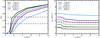 |
Fig. 6 Values of fCNM (left) and σturb (right) as a function of the initial condition n0, for different values of the large scale velocity vS (from 5 to 20 km s-1). The dotted lines frame the observational values of fCNM and σturb that we want to reproduce. |
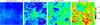 |
Fig. 7 Maps of column density (density integrated along the z-axis) displayed logarithmically. The initial density increases from the left to the right: n0 = 1.0, 1.5, 3.0, 10.0 cm-3. Turbulence forcing parameters are fixed to ζ = 0.5 at vS = 7.5 km s-1. All maps are displayed with the same column density range [6 × 1019 cm-2, 4 × 1021 cm-2]. |
All the simulations presented in this study have periodic boundary conditions. The velocity field is modified at every time step by the turbulent stirring in Fourier space (Sect. 2.2). The initial conditions correspond to a uniform and static WNM at a temperature of T = 8000 K. For a box size of 40 pc centered on z = 0, the profiles shown in Fig. 3 indicate that constant n and T are representative of the WNM.
This section presents the parametric study we did on the initial WNM density, n0, and on two properties of the stirring velocity field: the spectral weight, ζ, and the large scale velocity, vS. Overall we performed 90 simulations with 1283 cells, varying n0 from 0.2 to 10 cm-3, vS from 5 to 20 km s-1 and ζ from 0 (rotation free field) to 1 (divergence free). More specifically we explored the parameter space in two ways. First we looked at 48 simulations with variable n0 and vS, and a fixed ζ = 0.5 (Sect. 5.1). Then we investigate the effect of ζ and vS for a constant initial density of n0 = 1 cm-3 (Sect. 5.2). A test of the robustness of the results is presented and discussed in Sects. 5.3 and 5.4, where we compare these driven simulations to simulations with decaying turbulence.
Results of the 1283 simulations with natural turbulence ζ = 0.5.
5.1. Effect of the initial density
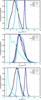 |
Fig. 8 Histograms of velocity dispersions: σtherm (top), σturb (middle) and σtot (bottom). On each panel, the different curves represent subsample of pixels selected according to their temperature: all pixels (black), the WNM (T> 5000 K, dark blue), the unstable gas (200 K<T< 5000 K, blue) and the CNM (T< 200 K, light blue). All quantities were computed using a high resolution simulation (10243 pixels) with the following initial conditions: n0 = 2.0 cm-3, ζ = 0.5 et vS = 7.5 km s-1. |
Table 1 and Fig. 6 present the results for 48 simulations for which the turbulence driving has been kept to a natural state (i.e., the ratio of compressible over solenoidal modes of the velocity field is kept in its initial state) using a fixed ζ = 0.5. For those simulations we only vary vS and n0. For each simulation we computed the CNM mass fraction fCNM, the mean Mach number ℳobs (Eq. (16)) and the mean velocity dispersion (Eq. (13)) at each Myr. In addtition we computed the average of those quantities over the time interval [20 Myr, 40 Myr] that corresponds to a period where a stationary state has been reached.
We observe that simulations with n0 between 0.2 and 1.0 cm-3 do not transit to cold gas. On the other hand, the efficiency of the CNM formation increases rapidly at higher values of n0. For n0 = 0.2 and 1.0 cm-3, the cold mass fraction is very close to zero while a small increase of the initial density (n0 = 1.5 cm-3) leads to fCNM= 0.3−0.4. Initial densities greater than 3.0 cm-3 lead to more than half of the mass to transit (see Fig. 6 left part). This behavior can be appreciated by looking at integrated density maps (Fig. 7). The map on the left, that corresponds to n0 = 1 cm-3, contains only WNM and is smooth. With the increase of n0, more and more contrasted structures appear, corresponding to the formation of CNM.
One can notice that n0 = 1.5 cm-3, the minimum initial density at which significant CNM is formed, corresponds to a pressure (12 000 K cm-3) much higher than the maximum pressure allowed for the WNM (see Sect. 3.1). At such high pressure and low density, the gas starts in the thermally unstable regime; it is indeed located above the stable branch of the WNM and in a zone of cooling that allows it to evolve rapidly and efficiently toward the cold phase.
We also note that the final turbulent velocity dispersion, σturb, is lower for higher values of n0 and therefore for higher values of the cold mass fraction fCNM (see Table 1 and Fig. 6). To first order, this can be understood by the fact that once a CNM structure is formed, it concentrates a fraction of the mass in a small volume. The velocity dispersion of this structure is lower than if the same amount of gas was spread out in the WNM on much larger scales (σturb ∝ lq). Because σturb is weighted by density (see Eq. (13)), its average value decreases when the amount of mass located in small scale structures increases, or equivalently when fCNM increases.
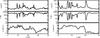 |
Fig. 9 Density, temperature and velocity (z-component) profiles for a given simulation (10243 cells, n0 = 2.0 cm-3, ζ = 0.5 et vS = 7.5 km s-1) and for two distinct lines of sight characterized by their value of CNM velocity dispersion: σturb(CNM) = 0.14 km s-1 (left) and σturb(CNM) = 4.7 km s-1 (right). |
Results of the 1283 simulations with initial density n = 1 cm-3.
To understand this behavior in more details, we studied the distributions of σturb, σtherm and σtot in a simulation at high resolution (10243 cells, n0 = 2.0 cm-3, ζ = 0.5 and vS = 7.5 km s-1). All distributions are plotted in Fig. 8, each velocity dispersion was computed using all pixels (black line) and also by selecting pixels corresponding to each thermal phase (CNM: T < 200 K, thermally unstable: 200 <T< 5000 K, WNM: T > 5000 K). As expected σtherm depends on the temperature of the gas. We note that it is also the case for the distributions of σturb, the one computed in the CNM being especially different from the other two. The distribution of σturb(CNM) peaks at very small values between 0.1 and 0.2 km s-1 with a tail reaching 5 km s-1. We recall that these velocity dispersions are computed by integrating along the line of sight (Eqs. (13), (17) and (18)). To better understand the shape of these distributions, we looked at two distinct lines of sight for which σturb(CNM) is equal to 0.14 and 4.7 km s-1 respectively. The density, temperature and velocity (z-component) profiles are plotted in Fig. 9. The line of sight with a low σturb(CNM) (Fig. 9 – top) is composed of four CNM structures with temperatures between 100 and 500 K. These clumps have homogeneous internal velocities and small relative velocities (about 3 km s-1). On the other hand, for the line of sight with a higher σturb(CNM) (Fig. 9 – bottom), the internal velocities of the CNM structures are also homogeneous, but their relative velocities are high, about 15 km s-1. This analysis indicates that individual clumps have an internal velocity dispersion of about 0.2 km s-1 (the peak at low values in the histogram of σturb(CNM)) and that high values of σturb(CNM) are the result of the relative velocities between clumps. Moreover, the similarities of the histograms of σtot and σtherm in Fig. 8 indicates that the velocity dispersion is dominated by thermal motions suggesting a subsonic Mach number. Like Heitsch et al. (2005, 2006) we conclude that the cold gas structures have subsonic internal motions and that the supersonic Mach number generally observed in the CNM (Heiles & Troland 2003) can be the result of their relative motions.
A similar explanation is proposed for the increase of the observed Mach number, ℳobs, with n0 and fCNM (see Table 1). The quantity ℳobs is the ratio of σturb to σtherm. With the increase of the amount of cold gas (i.e., fCNM), the average temperature of the box decreases proportionaly, as well as σtherm. Previously we have seen that σturb also decreases with fCNM but it does it more slowly than σtherm due to the contribution of clump relative motions inherited from the WNM.
We also note that, at a given n0, the efficiency of the CNM formation
decreases when the amplitude of the turbulence driving vS increases
(see Fig. 6 – left) and thus when the Mach number
increases, an effect also mentioned by Audit &
Hennebelle (2005). Sánchez-Salcedo et al.
(2002) and Vázquez-Semadeni et al. (2003)
argue that supersonic turbulence acts faster than TI and thus dominates the evolution of
the cloud, an explanation confirmed by Walch et al.
(2011). As stated in Eq. (6) and
as emphasized by Hennebelle & Pérault
(1999), the formation of CNM occurs when the radiative time is lower than the
dynamical time. Equivalently, the cooling time must be lower than the typical time of the
stirring: 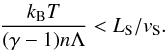 (19)For
fixed box size (LS) and initial temperature, this offers a
natural explanation why the transition is inefficient at the lowest densities and the
highest amplitudes vS.
(19)For
fixed box size (LS) and initial temperature, this offers a
natural explanation why the transition is inefficient at the lowest densities and the
highest amplitudes vS.
5.2. Effect of the compressive modes
Using isothermal simulations of molecular clouds, Federrath et al. (2008, 2010) showed that the ratio of compressible to solenoidal modes of the forced velocity field has an impact on the density structure of the gas. To understand the effect of the nature of the turbulent forcing on the CNM formation in the case of a thermally bistable gas, we performed 42 simulations (1283 pixels) with different values of the projection weight ζ and a fixed initial density n0 = 1.0 cm-3, close to the typical WNM density. We chose an initial density that we showed does not induce CNM formation in the case of the natural state of turbulent forcing (ζ = 0.5, see Sect. 2.2) in order to see if a different combination of compressive versus solenoidal modes can trigger the phase transition at low density. Like previously, the velocity field amplitude vS was varied from 5 to 20 km s-1. The velocity field is either purely compressive (ζ = 0), either purely solenoidal (ζ = 1) or a mixing of both components (0.1 ≤ ζ ≤ 0.9). Table 2 summarizes the values of ℳobs, ℳtheo, fCNM and σturb in the stationary regime for the 42 simulations. The behavior of fCNM and σturb with ζ are also presented in Fig. 10.
These results show that a turbulent field with a majority of solenoidal modes or with an energy equilibrium between compressible and vortical modes (ζ ≥ 0.5) cannot trigger the transition to CNM with n0 = 1 cm-3 (Fig. 10 – left). This behavior is obvious in the representations of the integrated density in Fig. 11: the more compressive modes the velocity field has, the more cold gas is formed. For a WNM initial density of n0 = 1 cm-3, ζ needs to be lower than 0.3 to reach 30% of the mass in the cold phase. Besides, as previously showed and for the same reason, fCNM increases at lower values of vS, for a given value of the spectral weight ζ (Fig. 10, – left).
We also note that σturb continually increases with the projection weight ζ (Fig. 10, –right), even when no cold gas is created in the simulation. The turbulent motions estimated with σturb are thus affected by their repartition in the compressive and solenoidal modes. σturb increases with the energy fraction injected in the solenoidal modes for the same total amount of energy injected. The solenoidal modes are efficient at mixing and uniformizing the density more efficiently than the compressive modes, which create higher density contrasts correlated with the velocity field (Federrath et al. 2010). The σturb computation gives more weight to the high density regions and thus to the compression regions where the velocity field is close to uniform, explaining why σturb decreases when the compressive modes become dominant. This illustrates that a higher fraction of compressible modes is not equivalent to a higher Mach number and emphasizes a clear difference with isothermal simulations (Federrath et al. 2008). The increase of the fraction of compressive modes is applied without increasing the amplitude of the velocity, and thus, without decreasing the crossing time, so that the gas has time to cool.
5.3. Robustness tests
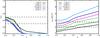 |
Fig. 10 Values of fCNM (left) and σturb (right) as a function of ζ, for different values of the large scale velocity vS (from 5 to 20 km s-1). The dotted lines frame the observational values of fCNM and σturb that we want to reproduce. |
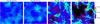 |
Fig. 11 Maps of column density (density integrated along the z-axis) displayed logarithmically. The projection weight decreases from the left to the right: ζ = 0.5, 0.4, 0.2 and 0.0. The initial density and the large scale velocity are fixed to n0 = 1.0 cm-3 and vS = 12.5 km s-1. All maps are displayed with the same column density range (3 × 1019 cm-2, 3.2 × 1021 cm-2). |
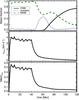 |
Fig. 12 Time evolution of the mass fraction in the CNM, WNM and thermally unstable gas (top), the mean Mach number ℳobs (middle), and the mean velocity dispersion σturb (bottom) for a decaying simulation with the following initial conditions: n0 = 1 cm-3, ζ = 1.0, vS = 7.0 km s-1. The turbulent driving was applied at first and shut down after 40 Myear. |
One concern often raised about simulations done using a sustained turbulent driving in Fourier space is how it affects the dynamics of the flow and, in the specific case of thermally bistable H i, how it affects the formation of cold structures. One might be concerned with the fact that compressive modes of the forcing, applied everywhere in space and at every time step, can create unrealistic expanding or compressive flows that could enhance or inhibit the formation of cold clumps. In addition, as emphasized by Avila-Reese & Vázquez-Semadeni (2001), the driving in the ISM is highly intermittent both in time and space, so another concern is that the continuous driving of turbulence might prevent the formation of cold structures altogether.
In order to test the robustness of our results, we produced low resolution simulations (1283 cells) in decaying mode and with a purely solenoidal driving (ζ = 1) to avoid the effect of compressive modes on the formation/destruction of clumps. To test the impact of the continous forcing on the transition, the forcing was turned off at 40 Myear and, after that point, the simulation continued during 80 Myear in decaying mode. We used three initial densities: n0 = 0.5, 1.0 and 2.0 cm-3 and the large scale amplitude of the forcing was fixed to vS = 7.0 km s-1. At the end (120 My), the Mach number is stabilized below 0.1, which is much lower than the observed value in the H i but allows the study of a complete decay.
Like for the forced turbulence simulations at n0 = 0.5 cm-3, the decaying simulation at n0 = 0.5 cm-3 does not create any CNM. This result addresses one main concern: it indicates that sustained turbulence forcing in Fourier space is not responsible for the lack of CNM in simulations with initial conditions representative of the WNM in the local ISM.
The high density case (n0 = 2.0 cm-3) produces CNM efficiently; it reaches fCNM = 0.35 while the turbulence is driven but, interestingly, the fraction of CNM increases significantly, up to fCNM = 0.8, when the forcing is stopped. This is due to the fact that, the turbulence being shut down, the Mach number decreases below 0.1 and the turbulent motions, becoming negligible, do not prevent the unstable gas to cool down anymore. This effect has also been observed by Walch et al. (2011).
One interesting case is the simulation with n0 = 1.0 cm-3. For this simulation, the evolution with time of the mass fraction of the different phases, ℳobs, and σturb are presented in Fig. 12. We previously showed that at this density, the driving must have a majority of compressible modes to trigger the formation of CNM. As expected, no CNM and no unstable gas are created here during the driven part. However, the mass fraction of CNM reaches 60% during the decaying part of the simulation. The decay of turbulence enables the formation of unstable gas at first, which itself transits to CNM after 20 My. This is very interesting in the context of a turbulence driving that would occur by short burst of energy injection. It suggests that such intermittent driving of turbulence could be efficient at forming CNM. The problem with this picture is that the CNM is formed slowly and late after the driving has been shut down. The amount of CNM reaches 30% only when the turbulent velocity dispersion and therefore the Mach number are much lower (σturb = 0.4 km s-1 and ℳobs = 0.06) than the measured values (3 km s-1 and 1.0).
Finally we wanted to push further the comparison between the two types of simulations (driven turbulence and decay) in a case where they are both in the same dynamical state. We looked at the properties of the decaying simulations at a time where the Mach number is 0.4 which corresponds to a time where the driving was stopped and the turbulence is decaying (see Fig. 12). We then selected sustained turbulence driving simulations with the same n0 and ζ = 1 that have ℳobs~0.4 in the stationary regime. For all values of n0, there are no significant difference in the CNM mass fraction for decaying and sustained turbulence simulations, indicating that the process responsible for the dynamical state of the gas has limited impact on the formation of cold structures.
From the tests we have made by comparing driven and decaying turbulence simulations, we conclude that using sustained turbulence driving in Fourier space is not biasing the results presented here on the formation of the CNM.
5.4. Discussion
-
1.
The first main result of the parameter studyon 1283 simulations is that the fiducial conditions of the WNM (n0 = 0.2–0.5 cm-3 and T = 8000 K) do not lead to the formation of cold gas, whatever the turbulence properties in the range we explored. With a slight increase of the density (n0 = 1 cm-3), a majority of compressive modes of the stirring are needed to trigger the transition. A higher increase of the initial WNM density (above n0 = 1.5 cm-3) produces CNM very efficiently. A moderate compression effect is therefore needed to trigger the transition with either a compressive velocity turbulent field or with an increase of the WNM density (or pressure). To first order the required increase in pressure (from P1 to P2) for the WNM-CNM transition could happen by the confluence of two flows with a relative velocity Δv:
![Mathematical equation: \begin{eqnarray} \Delta v = \left[(P_2-P_1)\left(\frac{1}{\rho_1}-\frac{1}{\rho_2}\right)\right]^{1/2}\cdot \end{eqnarray}](/articles/aa/full_html/2014/07/aa21113-13/aa21113-13-eq199.png) (20)Considering
n1 =
0.5 cm-3 (typical density in the WNM), n2 =
2.0 cm-3 (efficient to trigger the transition) and
T =
8000 K, one obtains Δv = 10.3 km s-1. The pressure increase
needed to place the WNM into suitable conditions to trigger the transition can
happen with converging flows with a relative velocity of 10 km s-1, which is reasonable in
cases of supernovæ explosions or stellar winds, and compatible with the idea that
turbulence on large scales is produced by converging flows induced by the star
formation activity (Ferrière 2001; Elmegreen & Scalo 2004; McKee & Ostriker 2007; de Avillez & Breitschwerdt 2007; Kim et al. 2010, 2011). That no CNM is formed at low density, whatever the forcing
conditions, can imply that typical turbulence motions only triggers the transition
of the WNM to CNM if such a transition can spontaneously occur in the medium, i.e.,
if the WNM is already in a thermally unstable state. This means that turbulence only
plays a role in the shaping of the cold medium. This is due to the density of the
WNM that is the result of the segregation of the medium into WNM and CNM. Therefore
the natural initial condition for the formation of CNM should not be the WNM density
but the average density of the ISM. This result would suggest that the formation of
CNM should be more efficient in the spiral arms.
(20)Considering
n1 =
0.5 cm-3 (typical density in the WNM), n2 =
2.0 cm-3 (efficient to trigger the transition) and
T =
8000 K, one obtains Δv = 10.3 km s-1. The pressure increase
needed to place the WNM into suitable conditions to trigger the transition can
happen with converging flows with a relative velocity of 10 km s-1, which is reasonable in
cases of supernovæ explosions or stellar winds, and compatible with the idea that
turbulence on large scales is produced by converging flows induced by the star
formation activity (Ferrière 2001; Elmegreen & Scalo 2004; McKee & Ostriker 2007; de Avillez & Breitschwerdt 2007; Kim et al. 2010, 2011). That no CNM is formed at low density, whatever the forcing
conditions, can imply that typical turbulence motions only triggers the transition
of the WNM to CNM if such a transition can spontaneously occur in the medium, i.e.,
if the WNM is already in a thermally unstable state. This means that turbulence only
plays a role in the shaping of the cold medium. This is due to the density of the
WNM that is the result of the segregation of the medium into WNM and CNM. Therefore
the natural initial condition for the formation of CNM should not be the WNM density
but the average density of the ISM. This result would suggest that the formation of
CNM should be more efficient in the spiral arms. -
2.
The second main result is that a sub or transonic turbulence is required to get CNM gas with properties in agreement with observations (fCNM ~ 40% and σturb ~ 3 km s-1). In opposition to an isothermal gas, it is rather inefficient to inject supersonic turbulence to produce high density structure in a thermally bistable turbulent flow. This result ties up with the idea of Vázquez-Semadeni et al. (2000), Sánchez-Salcedo et al. (2002) and Audit & Hennebelle (2005) that when tdyn is lower than tcool, turbulent compressions and depressions act quicker than the thermal instability, preventing its development. On the contrary, when tcool<tdyn, the gas cools down fast enough while turbulence is compressing it that it can reach the stable branch of the CNM before its reexpansion (Hennebelle & Pérault 1999). This argument is in agreement with previous studies. Walch et al. (2011) observed that effect with similations typical of the solar neighborhood physical conditions; they also found that the two phases appear only for low Mach number. Gazol et al. (2005) also mentioned that, as the Mach number increases, the ratio tcool/tdyn increases as well and the structures become transient and move away from the cold branch of the thermal equilibrium. Similarly, based on simulations of H i converging flows, Heitsch et al. (2005) observed that the thermal instability is efficient when the density is high and the velocity of the flow low.
-
3.
The third important result is related to the impact of the distribution of the turbulent energy between the solenoidal and compressive modes. Simulations with moderate initial WNM density (n0 = 1.0 cm-3) and purely compressive forcing field (ζ = 0) lead to a fraction of CNM close to what is deduced from observations, but in a very long time (>20 Myr). Besides, the Mach number and the turbulent velocity dispersion also need more than 10 Myr to converge to the observed values, suggesting that the turbulence takes a long time to be fully developed, namely to distribute the energy of the compressive modes toward the solenoidal modes. The convergence and the conversion of the WNM in CNM is much faster (~1 Myr) in the case of turbulence with a natural ratio of solenoidal to compressive modes but in this case a slightly higher WNM density (n0 > 1.5 cm-3) is required to trigger the transition. Given these timescales, we conclude that it is more likely that the formation of CNM structures occurs by an increase of the WNM density rather than purely compressive turbulent energy injection at lower density.
A second goal of this work was to study in details the scaling properties of turbulence as well as the properties of the CNM structures formed in a thermally bistable flow. To do so we produced two high resolution simulations (10243) with initial conditions selected from the results of the low resolution parametric study. The analysis of these two simulations is described in the next section.
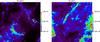 |
Fig. 13 Maps of column density (density integrated density along the z-axis) for 1024N01 (left) and 1024N02 (right). Units are 1020 cm-2. |
6. High resolution simulations
Two high resolution simulations (10243) were produced within the same framework as the parametric study (box size of 40 pc, turbulence driving in Fourier) with initial conditions identified previously as leading to H i properties close to the observed ones.
The first one (hereafter 1024N01) has an initial density of n0 = 1 cm-3, a majority of compressible modes with ζ = 0.2, and a large scale velocity vS = 12.5 km s-1. The second one (hereafter 1024N02) has an initial density of n0 = 2 cm-3, high enough to allow us to study the natural state of the turbulent velocity field with ζ = 0.5, and a large scale velocity vS = 7.5 km s-1. These two initial conditions lead to the formation of about 40% of cold gas, a subsonic Mach number and a turbulent velocity dispersion between 2 and 3 km s-1.
The initial densities chosen are higher than the observed density of the WNM (see Sect. 3.2) in accordance with our previous results showing that some compression of the WNM is needed in order to trigger the formation of CNM. On the other hand, as about 40% of the mass is converted to CNM with a volume filling factor of about 1%, the density of the WNM in the stationary regime is about 60% the initial value and therefore closer to the observed WNM density.
All the results presented hereafter concern these two 10243 cells simulations after 16 Myr. The integrated density along the z-axis of both simulations are shown in Fig. 13. These maps reveal structures in clumps and filaments comparable to what is seen in observations of the diffuse ISM. From this first look we already notice that 1024N02 creates more structures than 1024N01, suggesting that it is more efficient at triggering the transition. This will be discussed later.
6.1. Mach number
Properties of turbulence in the two high resolution simulations.
Table 3 summarizes the values of ℳtheo, computed on all the pixels and for pixels with T > 200 K, ℳobs, and σturb. The values of ℳtheo indicate that 1024N01 is subsonic while 1024N02 is transonic. Besides, removing the cold pixels (T < 200 K) from the computation does not change the results, suggesting that turbulent motions are dominated by the WNM motions, as we will discuss later. On the other hand, the values of ℳobs are clearly subsonic for both simulations, in agreement with observations. Lastly, both simulations reproduce very well the observed properties of σturb. In fact the computed values of σturb are slightly lower than the estimated value in a WNM cloud of 40 pc (~3 km s-1) but this is due to the cold structures present in the simulations for which the velocity dispersion is much lower.
6.2. Thermal distribution of the gas
Mass fraction f and volume filling factor φ of the three thermal phases: CNM, thermally unstable and WNM.
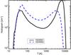 |
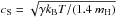
Fig. 14 Histogram of temperature weighted by density for 1024N01 (solid black line) and 1024N02 (dashed blue line). The histogram of 1024N02 was divided by 2 to be comparable to 1024N01. |
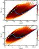 |
Fig. 15 Distributions of mass in a pressure-density diagram for 1024N01 (top) and 1024N02 (bottom). The unit of these density-weighted 2D histogram is the logarithm of the density (in cm-3). The solid blue curve shows the thermal equilibrium (cooling equal to heating), the dashed-dotted lines are isothermal curves at 200 K (green) and 5000 K (yellow). |
As expected with the thermal instability at low Mach number, the distribution of the gas in the P,n,T space presents the evidence of a multiphasic medium. The histograms of T (Fig. 14) have a clear bimodal shape, with a peak in the warm phase and one in the cold phase. Similarly the mass distribution of the gas in the P − n diagram (Fig. 15) shows two preferential zones: the first one at high density and the second one at low density, suggesting again CNM and WNM.
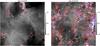 |
Fig. 16 Maps of log 10(n) for 1024N01 (left) and 1024N02 (right). These maps are 2D slices in the 3D density cubes, taken at a time where the simulations have reached a stationary state. The contours are from the corresponding temperature cubes indicating frontiers at 200 K (blue lines) and 2000 K (red lines). |
However, the thermal properties of the warm gas are slightly different in both simulations. If the histograms of T of the cold gas peaks at similar temperatures in both cases (40 K for 1024N01 and 50 K for 1024N02), it is not true for the warm gas: while the WNM of 1024N01 has ⟨ T ⟩ ~ 7000 K, close to the prediction of the two-phase model (Field et al. 1969), the warm gas in 1024N02 has ⟨ T ⟩ ~ 3500 K. This effect can also be seen in the pressure-density diagrams (Fig. 15), where the pressure of 1024N02 is lower than the one of 1024N01 at low densities. Therefore, while the gas at low density of 1024N01 follows the stable branch of the WNM, the gas at low density of 1024N02 is shifted below the equilibrium curve where the heating is dominant. This pressure difference is confirmed by the histograms of P presented in Fig. 17, where the mean pressure of 1024N02 (right) is lower than the mean pressure of 1024N01 (left). On the other hand, the histograms of n presented in Fig. 18 peaks around 0.5−0.6 cm-3 in both cases, similar to the WNM mean density estimated from observations.
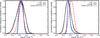 |
Fig. 17 Histograms of pressure for 1024N01 (left) and 1024N02 (right): three dimensional pressure (black), averaged pressure along the line of sight (blue). The associated colored dashed lines are lognormal fits. The red dashed-dotted line represent the lognormal fit found by Jenkins & Tripp (2011) on observations. The lognormal coefficients ([a1, a2] – see Eq. (21)) are [3.58, 0.175] for Jenkins & Tripp (2011). For the 3D and averaged pressure, they are [3.58, 0.29], [3.58, 0.14] for 1024N01 and [3.35, 0.20], [3.38, 0.09] for 1024N02. |
Two factors can be considered to explain the presence of warm gas out of equilibrium. First, a higher initial density decreases the WNM cooling time (Eq. (8)): tcool goes from 1.75 Myr for n0 = 1.0 cm-3 to 1.15 Myr for n0 = 2.0 cm-3. Therefore, the warm gas located below the equilibrium in 1024N02 is cooled down faster than in 1024N01 and does not have time to reach the equilibrium curve. Secondly, the thermal equilibrium curve considered in the P − n diagram is established for a static gas and does not take the energy contribution of turbulence into account. Depending on the properties of the turbulence, WNM gas can stabilized at a temperature significantly lower than the prediction of the two-phase model.
The definition of the H i thermal phases in the physical parameter space is not always clear in the litterature; it depends somewhat if they are looked at from the simulation or the observation perspective. Here we used three criteria to estimate the mass fraction of the CNM, WNM and thermally unstable gas, based on T and n thresholds. All results are summarized in Table 4.
Whatever criteria we used to estimate the CNM (T or n), the fraction of the total mass in the CNM is 30% and 50% for 1024N01 and 1024N02 respectively. These quantities are in good agreement with the results obtained with the same conditions but on a 1283 grid, providing another validation of the use of low-resolution simulations for parameter space exploration. These values of fCNM are also in agreement with observational results: Heiles & Troland (2003) estimated that 40% of the mass of the H i lies in the cold phase using 21 cm emission and absorption measurements, and we found fCNM~ 44% based on large scale properties of the H i emission (see Sect. 3.4). The CNM volume filling factor found in these high resolution simulations (1% for 1024N01 and 4% for 1024N02) are also representative of what we estimated from observations.
The estimate of the mass in the WNM and thermally unstable gas depends significantly on the criteria used. One way to separate the phases is to use the density thresholds that define the range of the thermally unstable gas, as described in Sect. 3.1 (see the dash-dotted lines in Fig. 2). Using that criteria, both simulations hold the same amount of unstable gas (~30%), the difference between the two simulations only lies in the CNM and WNM phases: the amount of gas that does not transfer to CNM in 1024N01 stays in the WNM phase. We note that in the case of 1024N01, the three thermal phases are distributed like 1/3–1/3–1/3, as observed by Heiles & Troland (2003), while in the 1024N02 case, the mass fraction of WNM is lower of a factor 2 and 50% of the mass is in the CNM.
One can also estimate the mass fraction of the WNM and thermally unstable gas using a threshold in T. In both simulations we found that about 20% of its mass is lying between 2000 and 5000 K. In 1024N02, where the WNM-CNM transition is highly efficient, the unstable regime holds the major part of the mass (46% between 200 and 5000 K) and half of it has a temperature lower than 2000 K; in 1024N01, where the WNM-CNM transition is less efficient, only 10% is lying between 200 and 2000 K and a significant amount of the gas lies in the WNM range beyond 5000 K (40%).
Finally it is interesting to look at the spatial distribution of the three phases. In Fig. 16 we present 2D density slices for each simulation with isocontours placed at 200 K (blue) and 2000 K (red). The highest temperature threshold has been consciously chosen lower than the usual limit at 5000 K in order to see the distribution of the thermally unstable gas. The gas lying between 2000 and 5000 K is widely distributed and does not show any preferential location. On the other hand, the thermally unstable gas below 2000 K lies preferentially around the cold structures as sheets around the denser regions, in agreement with Gazol & Kim (2010).
6.3. Pressure range
Jenkins & Tripp (2011) used UV absorption measurements of neutral carbon observed in front of stars to study the distribution of the thermal pressure in the diffuse, CNM. They found that the pressure distribution, weighted by the mass density, is well fitted by a lognormal. It is also the case for our two high-resolution simulations. Figure 17 shows the histogram of P weighted by n (black line) and the average pressure along the line-of-sight weighted by density in each cell (blue line), this quantity being closer to what is measured with real observations for which the 3-dimensional pressure is not available. For comparison purpose, the pressure distribution found by Jenkins & Tripp (2011) is also shown in these plots (red dotted line).
The pressure histograms of Fig. 17 were fitted with
a lognormal, following the definition of Jenkins &
Tripp (2011): 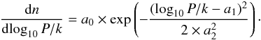 (21)The
values found for our lognormal fits are given in the caption of Fig. 17. The simulation 1024N01 peaks at 3800 K cm-3 (3.58 dex), the same value
found by Jenkins & Tripp (2011). The
pressure peak of 1024N02 is slightly lower at 2200 K cm-3 (3.34 dex). These two values
lie in the pressure range allowing a two-phase medium. We point out that the width of the
histograms are broader for the 3D pressure histograms than for the averaged pressure in
both cases (0.29 and 0.20 dex compared to 0.14 and 0.09 dex respectively) due to the
average along the line of sight that compresses the dynamical range. In addition, the
distributions of 1024N01 are wider than those of 1024N02, which can be explained by the
higher amplitude of the turbulent stirring used in 1024N01. In any case, the widths of the
pressure histrograms stay close to the result of Jenkins
& Tripp (2011) and are thus in good agreement with the observations.
(21)The
values found for our lognormal fits are given in the caption of Fig. 17. The simulation 1024N01 peaks at 3800 K cm-3 (3.58 dex), the same value
found by Jenkins & Tripp (2011). The
pressure peak of 1024N02 is slightly lower at 2200 K cm-3 (3.34 dex). These two values
lie in the pressure range allowing a two-phase medium. We point out that the width of the
histograms are broader for the 3D pressure histograms than for the averaged pressure in
both cases (0.29 and 0.20 dex compared to 0.14 and 0.09 dex respectively) due to the
average along the line of sight that compresses the dynamical range. In addition, the
distributions of 1024N01 are wider than those of 1024N02, which can be explained by the
higher amplitude of the turbulent stirring used in 1024N01. In any case, the widths of the
pressure histrograms stay close to the result of Jenkins
& Tripp (2011) and are thus in good agreement with the observations.
6.4. Density histograms
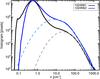 |
Fig. 18 Histograms of density for 1024N01 (black) and 1024N02 (blue). The dashed lines are lognormal fits of the high density part. |
The density distribution is of great importance in turbulence studies. Many simulations of molecular clouds have shown that the density distribution of an isothermal gas follows a lognormal law with a widening that depends on the Mach number (Vázquez-Semadeni 1994; Passot & Vázquez-Semadeni 1998; Federrath et al. 2008). The density distribution of a two-phase gas is however more complex and often presents a bimodal shape (Hennebelle et al. 2008; Audit & Hennebelle 2005, 2010). Vázquez-Semadeni et al. (2000), Piontek & Ostriker (2005), Gazol et al. (2005) and Walch et al. (2011) showed that density histograms are broadened and loose the bimodal shape when the Mach number increases, as most of the gas moves to the thermally unstable regime. The density distributions presented in Fig. 18 point to the evidence of a transonic biphasic gas with two distinct peaks, one at low densities, 0.4–0.5 cm-3, typical of the WNM, and a second one around 10–20 cm-3, representative of the CNM.
To compare with studies of molecular clouds, we tried to fit lognormals on the cold peaks for each simulation. Regarding the high density part, it is possible to fit the right tail with a lognormal, but for both simulations, the lognormals are overly broad. To study this further, we separated the cells of the box where T < 200 K and plotted the histogram of the CNM density. They did not show any characteristic shape, and it was impossible to fit lognormals on them. We also didn’t find any evidence of a power law tail as Seifried et al. (2011) did. Therefore, even though a lognormal fit is possible on the high density part of the histogram, it is difficult to make any physical interpretation out of it.
6.5. Power spectra
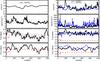 |
Fig. 19 Statistical properties of n and vz for each slice of the cube along the z-axis: isothermal simulation (left) and TI simulations (right, black is 1024N01 and blue is 1024N02). From top to bottom: density contrast, maximum density, 2D power spectra slopes of density (Pk(n)) and velocity (Pk(vz)). The red dashed lines indicate the expected power spectrum slope for Kolmogorov type turbulence. |
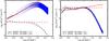 |
Fig. 20 Compensated power spectra Pkk2.67 for n (left) and vz (right) computed on 1024N01 (black solid line) and on the isothermal simulation (black dashed line). The red lines indicate the power law fits done on the range of k given in Table 5. These power spectra are the average of all the Pk computed on each slices along the z-axis (see Fig. 19). The blue error bars indicate the dispersion at each k value. |
Compared with converging flow simulations, the stirring in Fourier provides a wider range of scales over which the properties of turbulence can be studied. In particular, such simulations offer an opportunity to better study the velocity and density power spectra and therefore characterize some specific properties of a turbulent and thermally bistable medium. In this section we present a study of the statistical properties of the density and velocity fields of 1024N01 and 1024N02. For comparison purposes, we also made the same analysis on an isothermal simulation of 10243 cells, obtained with the same turbulent stirring than 1024N01 (ζ = 0.2 and vS = 12 km s-1), an initial conditions of n0 = 1 cm-3 and T = 8000 K. This simulation is subsonic with a Mach number equal to 0.9.
For each 2D plane perpendicular to the z-axis, we calculated the density contrast σ(n)/⟨ n ⟩, the maximum of the density and the slope of the 2D power spectra of the density and the velocity. All quantities were computed for the set of points on each 2D plane perpendicular to the z-axis. The choice of the axis is not important as the simulations are isotropic due to the turbulent stirring in Fourier space. The advantage of computing quantities for each 2D plane is that it offers a way to quantify their variations across the cube. For a scalar field like the density, the power spectrum of 2D slices is equivalent to the power spectrum of the 3D cube (Miville-Deschênes et al. 2003b)3. We chose to compute the statistics of one component of the velocity (vz) and not its norm to stay closer to spectro-imagery observations that give only access to the velocity component along the line of sight. We also chose not to do the statistics of 21 cm velocity channel maps as their structure is a mixture of velocity and density fluctuations, especially in high density contrast media (Esquivel et al. 2007).
Power spectrum analysis of n and vz for three 10243 simulations.
The density contrast, the maximum density, and the slopes of the power spectra as a function of z, are shown for the isothermal and TI simulations in Fig. 19. We also computed the mean power spectra of the density and the velocity, by taking the mean of the 1024 power spectra computed on each plane perpendicular to the z-axis. Figure 20 shows these compensated mean power spectra k8 / 3P(k) for 1024N01 and for the isothermal simulation (the power spectra for 1024N02 being similar to those of 1024N01, they are not displayed here). The errors bars represent the (1σ) variations on the 1024 slices.
The estimation of the slope of the power spectrum in the inertial zone of numerically
simulated turbulence can only be done on a small scale range due to the turbulent forcing
on large scales and the numerical dissipation at small scales. We evaluated the inertial
range [
kmin,kmax
] for each mean power spectrum by minimizing the root mean square of
the error 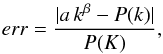 (22)where
a and
β are the
two parameters obtained with the power law fit. The size of the simulations
(10243) allows us
to expect at least a decade on which a power law fit is suitable. Therefore we imposed the
following condition on kmin and kmax:
kmax ≥ 10 ×
kmin. The slopes β as well as the
k-ranges
used for the different power spectra are summarized in Table 5.
(22)where
a and
β are the
two parameters obtained with the power law fit. The size of the simulations
(10243) allows us
to expect at least a decade on which a power law fit is suitable. Therefore we imposed the
following condition on kmin and kmax:
kmax ≥ 10 ×
kmin. The slopes β as well as the
k-ranges
used for the different power spectra are summarized in Table 5.
The density power spectrum of the isothermal and subsonic simulation has a slope of –8/3, which corresponds to the Kolmogorov estimation in 2D (see Elmegreen & Scalo 2004). This Kolmogorov law is in agreement with the previous results of Kim & Ryu (2005) and Kritsuk et al. (2007) who emphasized that subsonic and isothermal simulations have a Kolmogorov behavior. Regarding the TI simulations, the density power spectra are far from Kolmogorov with slopes of –1.3 for 1024N01 and –1.5 for 1024N02. This is due to the much higher density contrast. Its values are indeed around 4 (⟨ Cn01 ⟩ = 4.6 ± 1.4 and ⟨ Cn02 ⟩ = 3.8 ± 0.7) while the density contrast of the isothermal simulation is almost constant from slice to slice with a value of about 0.6 (Fig. 19 – left).
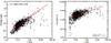 |
Fig. 21 Scaling relations for cold clumps: mass versus size (left) and 3D velocity dispersion versus size (right). The velocity dispersion of each clump is computed using the norm of the velocity field. Each plot was fitted with a power law, shown in red. |
As expected, the velocity power spectrum of the isothermal and subsonic simulation also follows the Kolmogorov estimation. However, the velocity power spectra of the two TI simulations are slightly flatter from Kolmogorov with slopes of –2.4 for 1024N01 and –2.3 for 1024N02.
In supersonic turbulent flows it is generally observed that the slope of the density power spectrum flattens with the increase of the Mach number. This effect has been reported for isothermal (Kim & Ryu 2005) and supersonic, thermally bistable (Gazol & Kim 2010) flows. It was also noted by Kritsuk et al. (2007) that the velocity power spectrum goes from Kolmogorov-like to Burgers-like when the Mach number increases. We observe that the density power spectrum of transonic, thermally bistable turbulence has the same behavior than for supersonic turbulence. On the other hand, while the velocity power spectrum of supersonic flows goes from Kolmogorov to Burgers turbulence (Kritsuk et al. 2007), the velocity power spectra in our case stay similar to the one of a subsonic flow with a slope close to Kolmogorov. In fact the velocity power spectra of the TI simulations are even slightly flatter than Kolmogorov, which is the opposite behavior expected for Burgers turbulence. Hennebelle & Audit (2007) emphasized that the density fluctuations of the H i, and thus the density contrast, are due to the thermal instability at low Mach numbers while supersonic shocks dominate at high Mach numbers. The TI simulations are indeed much more structured on the small scales than subsonic isothermal flows. We also want to point out that the power spectrum of the logarithm of the density, which traces more directly the velocity power spectra through the equation of continuity, has a slope very close to the Kolmogorov law for both 1024N01 and 1024N02.
6.6. CNM structures
Two observational facts often attributed to the self-similarity induced by the turbulent
cascade in the ISM are the mass-scale (M ∝ Lα
– Larson 1981; Elmegreen & Falgarone 1996; Roman-Duval
et al. 2010) and velocity dispersion-scale (σturb =
σ1
pcLγ – Larson 1981; Heyer
& Brunt 2004) relations observed in molecular clouds. If CNM clumps are
the precursors of molecular gas, it is interesting to see if they follow similar laws. To
identify CNM clumps in the simulations we selected pixels having a density greater than
5 cm-3.
Structures were then identified as spatially connected pixels in 3D. Following the
approach of Hennebelle et al. (2007), the size of a
structure is defined using the highest eigenvalue λ1 of its
inertial matrix ℐ:
![Mathematical equation: \begin{eqnarray} I_{ii} &=& \int(x_j^2+x_k^2) \mathrm{d}m \\ I_{ij} &=& \int{x_ix_j \mathrm{d}m} \\ I_{ji} &=& I_{ij} \quad \mathrm{with}\quad i,j,k \in [1,2,3]\quad\mathrm{and}\quad i\ne j\ne k. \end{eqnarray}](/articles/aa/full_html/2014/07/aa21113-13/aa21113-13-eq266.png) The
xi, i ∈ {
1,2,3 }, are the pixels coordinates
and dm the
infinitesimal mass. One can thus estimate the size of the structure by computing
The
xi, i ∈ {
1,2,3 }, are the pixels coordinates
and dm the
infinitesimal mass. One can thus estimate the size of the structure by computing
 ,
where M is
its mass. We point out that Audit & Hennebelle
(2010) investigated other choices than the highest eigenvalue (the geometrical
mean of the eigenvalues for instance) and found very similar results.
,
where M is
its mass. We point out that Audit & Hennebelle
(2010) investigated other choices than the highest eigenvalue (the geometrical
mean of the eigenvalues for instance) and found very similar results.
Figure 21 – left shows the relation between M and L for the cold structures of 1024N01 (this relation for 1024N02 being similar to that of 1024N01, it is not displayed here). There is significant dispersion in this diagram but the points suggest a power law fit. We found slopes of 2.25 ± 0.05 and 2.28 ± 0.03 for 1024N01 and 1024N02 respectively. These results are in agreement with previous works on isothermal (Kritsuk et al. 2007; Federrath et al. 2009) and TI simulations (Audit & Hennebelle 2010). They are also similar to the results obtained on CO observations by Elmegreen & Falgarone (1996) who found slopes between 2.2 and 2.5 on a large sample of independent molecular clouds. Recently, Roman-Duval et al. (2010) measured an index of 2.36 on 580 molecular clouds. The structure observed here on H i simulations is thus similar to molecular clouds4.
Similarly we investigated the relation between the velocity dispersion and the size of
the CNM clumps. The velocity dispersion is computed as:
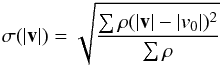 (26)with
v0 the mean velocity of each structure
weighted by density:
(26)with
v0 the mean velocity of each structure
weighted by density: 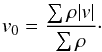 (27)Figure
21 (right) shows the values of σ( | v |)
versus L for
the structures of 1024N01 (1024N02 shows similar results). The power law fits give
0.70 ×
L0.41 and 0.51 × L0.42 for
1024N01 and 1024N02 respectively. We note the presence of a scatter of one order of
magnitude around the fitted power law, as it as been previously noticed on simulations by
Vázquez-Semadeni et al. (1997) and on
observations by Falgarone et al. (1992). Keeping in
mind that the slopes obtained here (0.41 and 0.42) may be subject to high uncertainty,
they are compatible with the results of Audit &
Hennebelle (2010) who found 0.33
< γ <
0.53. They are also close to values measured on observations: 0.37 in
H i clouds (Larson 1979) and molecular
clouds (Larson 1981), and 0.5 obtained on a large
sample of molecular clouds by Heyer & Brunt
(2004). On the other hand, the values obtained here for σ1 pc, 0.70 and
0.51 km s-1, are
lower than the results presented by Audit &
Hennebelle (2010) who found values between 1.2 and 3.3 km s-1 but with a different forcing
scheme. The turbulence in their simulation is indeed produced by WNM converging flows with
a Mach number close to 1.5. This type of forcing is very efficient to create cold
structures but induces a Mach number in the WNM higher than the one observed in the
diffuse ISM.
(27)Figure
21 (right) shows the values of σ( | v |)
versus L for
the structures of 1024N01 (1024N02 shows similar results). The power law fits give
0.70 ×
L0.41 and 0.51 × L0.42 for
1024N01 and 1024N02 respectively. We note the presence of a scatter of one order of
magnitude around the fitted power law, as it as been previously noticed on simulations by
Vázquez-Semadeni et al. (1997) and on
observations by Falgarone et al. (1992). Keeping in
mind that the slopes obtained here (0.41 and 0.42) may be subject to high uncertainty,
they are compatible with the results of Audit &
Hennebelle (2010) who found 0.33
< γ <
0.53. They are also close to values measured on observations: 0.37 in
H i clouds (Larson 1979) and molecular
clouds (Larson 1981), and 0.5 obtained on a large
sample of molecular clouds by Heyer & Brunt
(2004). On the other hand, the values obtained here for σ1 pc, 0.70 and
0.51 km s-1, are
lower than the results presented by Audit &
Hennebelle (2010) who found values between 1.2 and 3.3 km s-1 but with a different forcing
scheme. The turbulence in their simulation is indeed produced by WNM converging flows with
a Mach number close to 1.5. This type of forcing is very efficient to create cold
structures but induces a Mach number in the WNM higher than the one observed in the
diffuse ISM.
In order to compare σ1
pc to the work of Wolfire et
al. (2003) and to the value 0.92 km s-1 estimated in Sect. 3, we computed  for each CNM structure using the theoretical value γ = 1/3
expected for subsonic turbulence. The histograms of σ(1) presented in Fig.
22 peak around 0.8 and 0.6 km s-1 for 1024N01 and 1024N02
respectively. These values are in agreement with the velocity dispersion at 1 pc we wanted
to reproduce in these simulations and with the work of Wolfire et al. (2003). That σ1 pc is well reproduced suggests that
the internal dynamics of the CNM clumps is related to the dynamics in the WNM. To confirm
this assertion, we computed the mean velocity dispersion ⟨ σ( | v |)
⟩ (i.e. the average over all cold structures of their individual
turbulent velocity dispersion). We obtained 0.3 and 0.4 km s-1, much lower than the mean
thermal velocities of the clumps: 1.7 km s-1 for 1024N01 and 1.3 km s-1 for 1024N02. The individual
cold structures are therefore subsonic. On the other hand, the relative motions between
the clumps are greater. We computed the cloud-cloud velocity dispersion as
for each CNM structure using the theoretical value γ = 1/3
expected for subsonic turbulence. The histograms of σ(1) presented in Fig.
22 peak around 0.8 and 0.6 km s-1 for 1024N01 and 1024N02
respectively. These values are in agreement with the velocity dispersion at 1 pc we wanted
to reproduce in these simulations and with the work of Wolfire et al. (2003). That σ1 pc is well reproduced suggests that
the internal dynamics of the CNM clumps is related to the dynamics in the WNM. To confirm
this assertion, we computed the mean velocity dispersion ⟨ σ( | v |)
⟩ (i.e. the average over all cold structures of their individual
turbulent velocity dispersion). We obtained 0.3 and 0.4 km s-1, much lower than the mean
thermal velocities of the clumps: 1.7 km s-1 for 1024N01 and 1.3 km s-1 for 1024N02. The individual
cold structures are therefore subsonic. On the other hand, the relative motions between
the clumps are greater. We computed the cloud-cloud velocity dispersion as
 (28)where
N is the
number of clumps. We obtained σcc = 2.3 km s-1 for 1024N01 and
σcc =
1.9 km s-1. These values are very close to the total velocity
dispersions in the boxes (2.8 km s-1 for 1024N01 and 2.2 km s-1 for 1024N02), suggesting again
that the clump motions are related to the motions in the WNM. This means that the CNM
structures keep the memory of the flow in which they were formed and that little
dissipation occurs in cloud-cloud collisions.
(28)where
N is the
number of clumps. We obtained σcc = 2.3 km s-1 for 1024N01 and
σcc =
1.9 km s-1. These values are very close to the total velocity
dispersions in the boxes (2.8 km s-1 for 1024N01 and 2.2 km s-1 for 1024N02), suggesting again
that the clump motions are related to the motions in the WNM. This means that the CNM
structures keep the memory of the flow in which they were formed and that little
dissipation occurs in cloud-cloud collisions.
Part of this relation between CNM and WNM motions could be attributed to the turbulent forcing being applied as an acceleration instead of a force. In the context of a two-phase medium this might introduce biases, in particular an overestimate of the clump-to-clump velocity, because dense clumps are subject to the same accelerations as diffuse gas in the warm medium. Nevertheless, similar velocity dispersion of CNM and WNM structures were also reported by Heitsch et al. (2005, 2006) who simulated the formation of molecular clouds from H i converging flows and therefore did not use turbulent forcing in Fourier. Like them, we thus conclude that a significant fraction of the observed 21 cm line broadening is due to the relative motions of the clumps and is not the result of internal supersonic motions.
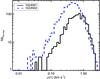 |
Fig. 22 Histogram of σ(vz) /L1 / 3 for the cold clumps identified in 1024N01 (black) and 1024N02 (blue). |
6.7. Summary and discussion
Here we summarize the physical properties of the CNM deduced from the analysis of two TI simulations at high resolution (10243, box size of 40 pc, resolution of 0.04 pc).
-
1.
First we showed that these simulations reproducewell all the observed physical quantities used as con-straints for the parametric study: a cold mass fraction ofabout 40%, a CNM volume filling fac-tor of 1 to 4%, a transonicMach number and a turbulent velocity dispersion ofabout 3 km s-1.Furthermore, like in the observations reported by Heiles &Troland (2003), about 1/3of the gas is in the thermally unstable regime. This re-sult also agrees with the previous works on simulationsof Gazol et al. (2005)and de Avillez & Breitschw-erdt (2005). Finally, the pressures are invery good agreement with the observations of Jenkins &Tripp (2011), both for the mean and the disper-sion.
-
2.
We noted that the thermally unstable gas, defined with temperatures between 200 and 5000 K behave in two different ways, depending on its temperature. The gas between 200 and 2000 K is located at the interface of the cold clumps and the warm gas while the gas beyond 2000 K is dynamically connected to the WNM and is widely distributed in the box. This wide distribution of the unstable gas temperature has also been noticed by Gazol & Kim (2010) who observed that the boundaries between CNM and WNM are sharper when the Mach number is very low (0.2), due to the unperturbed development of the thermal instability by turbulence. This is a natural consequence of the clumps being dynamically formed by locally converging motions. The gas is cooling while approaching the clumps, it is therefore natural that the coldest unstable gas is located around them.
-
3.
The density distribution is bimodal, bearing the characteristic of a bistable gas, as noticed by several authors (Vázquez-Semadeni et al. 2000; Audit & Hennebelle 2005; Gazol et al. 2005; Piontek & Ostriker 2004; Audit & Hennebelle 2010). This is a result of the gas being transonic. Indeed, a higher turbulence would maintain the gas in the thermally unstable regime (Gazol et al. 2005; Walch et al. 2011) and break the bimodality of the distribution that tends to be close to a single peak lognormal function. As mentioned by Sánchez-Salcedo et al. (2002) and Vázquez-Semadeni et al. (2003), this is due to the fact that for strong turbulence, the gas is not in the thermal equilibrium locus of the pressure-density phase diagram but is rather mostly in the thermally unstable range. This might not be representative of the solar neighborhood where the WNM is thought to be transonic, implying a bimodal histogram of the density. In this context, we tried to describe the high density part of the density histogram with a lognormal or a power law tail but showed that none of them were convincing.
-
4.
The 2D velocity power spectra of the simulations with thermal instability have slopes equals to –2.4 and –2.3 for 1024N01 and 1024N02 respectively, close to the Kolmogorov law (–8/3). On the other hand, the density power spectra are much flatter (–1.3 and –1.5) and the density contrasts are high (around 4). These signatures are the direct result of the formation of dense structures by the thermal instability in a low Mach number flow (Hennebelle & Audit 2007). We point out that the density power spectra computed on the TI simulations are similar to the one seen in supersonic isothermal flows where the density power spectrum flattens with the increase of the Mach number (Kim & Ryu 2005) while the velocity power spectra are characteristic of subsonic turbulence with a Kolmogorov slope.
-
5.
Cold clumps with a density higher than 5 cm-3 follow a mass-scale relation M ∝ Lα, with α = 2.25 and 2.28, in good agreement with observations (Elmegreen & Falgarone 1996; Roman-Duval et al. 2010) as well as with previous numerical studies, even when different conditions and algorithm are used (Kritsuk et al. 2007; Federrath et al. 2009; Audit & Hennebelle 2010). The cold clumps also follow a velocity dispersion-scale relation (σ ∝ Lγ) with γ = 0.41 and 0.42. These values are similar to the ones obtained on numerical simulations (Audit & Hennebelle 2010), to the observed in molecular clouds (Larson 1981; Heyer & Brunt 2004), but also to the value expected for a subsonic turbulence γ = 1/3. These results suggest that the self-similar density structures observed in molecular clouds could be inherited from the H i from which they were formed.
-
6.
The comparison of the internal velocity dispersion of the cold structures (0.3–0.4 km s-1) with their thermal velocity dispersion (1.3–1.7 km s-1) indicates that they are clearly subsonic. The turbulent velocity dispersion of clumps increases with scale with a normalization at 1 pc of σ(1) = 0.6−0.8 km s-1, very close to the value found in the WNM. Similarly, the cloud-cloud velocity dispersion is 1.9–2.3 km s-1, close to the total velocity dispersions in the boxes (2.2–2.8 km s-1). This implies that the turbulent motions inside clumps and the relative velocities between them are related to the motions of the WNM from which they were formed. Individually, the clouds are subsonic but their relative velocities are supersonic relative to the CNM sound speed (in accordance with Koyama & Inutsuka 2002; Heitsch et al. 2005). This result is in complete agreement with the work of Hennebelle & Audit (2007) who noticed that the CNM velocity dispersion estimated from 21 cm spectra is greater than the mean velocity dispersion of the CNM structures identified in their simulation. This means that a non negligible fraction of the measured velocity dispersion is caused by the relative motions of the clumps along the line of sight, suggesting that the observed line broadening is likely to be due to the relative clumps motions rather than supersonic turbulence.
7. Conclusion
We have presented a set of 90 low resolution simulations (1283 pixels) in order to study the physical conditions that lead to the production of CNM structures out of purely WNM gas, given the known observational constraints (velocity dispersion, density, pressure) of the H i in the local ISM and based on the model of the heating and cooling processes of Wolfire et al. (1995, 2003). These simulations show that WNM gas at typical values of density, temperature and turbulent motions do not transit to CNM gas. The typical volume density of the WNM in the disk at the position of the Sun lies between 0.2 and 0.5 cm-3. We showed that WNM with initial density under 1 cm-3 never transit into a cold phase, whatever the amplitude or the nature of turbulent motions. Stronger turbulent motions clearly does not help in producing cold gas, in fact we showed that it is the opposite. On the other hand a moderate increase of the WNM density (or equivalently of its pressure) is very efficient; all simulations with an initial density higher than 1.5 cm-3 do transit and the amount of cold gas in the simulation increases with the density. When the initial density reaches 3 cm-3, all simulations achieve to create at least 90% of CNM. These results were obtained with a natural balance between compressive and solenoidal modes in the injected velocity field. In this case the formation of CNM gas is almost instantaneous as soon as the turbulence is fully developed. We also explored the case of an intermediate initial density (1 cm-3) with a variation of the ratio of solenoidal to compressive mode in the turbulent forcing. We showed that, at this density, the transition into CNM only occurs when there is a majority of compressible modes in the turbulent velocity field but this process is much slower (10–20 Myr).
We conclude that the ISM turbulence cascade on its own cannot induce a transition from WNM into CNM at the average density of the WNM. The production of CNM is likely to be due to turbulent motions of moderate amplitude associated to a compressive event of the WNM that could be led by transient phenomena such as outflows, supernova explosion or spiral density waves. This would trigger the phase transition without delay. Once formed, the amount of CNM gas is dynamically stable. Therefore there is no need for a constant energy injection to maintain the high density contrast of the H i.
We also have presented a detailed study of the H i based on two higher resolution simulations (10243 pixels). To our knowledge these are the largest simulations to date that include the thermal instability and a pseudo-spectral turbulent stirring. The bimodal temperature and density histograms show the evidence of a bistable medium and the mass fractions of each phase, the Mach number of the WNM, and the pressure distributions are all in agreement with observations. With these simulations we confirm a number of results of previous studies based on converging flows (Heitsch et al. 2006; Hennebelle & Audit 2007; Audit & Hennebelle 2010) that showed that the structure of the CNM and WNM are tightly interwoven: the two media share the same velocity fields and the CNM cloud-cloud velocity dispersions is close to the WNM sound speed. While the individual CNM structures are clearly subsonic, their relative motions are supersonic with respect to their own temperature. In addition, thanks to the pseudo-spectral forcing method, the statistical properties of the turbulent bistable flow could be analyzed on a wider range of scales than could be done in previous studies. We found that for such subsonic or transonic bistable flows, the velocity field keeps the properties of subsonic turbulence with a power spectrum close the Kolmogorov while the density is highly contrasted, reminiscent of what is observed for supersonic flows and in molecular clouds. In the case of the H i simulated here, the joined action of the turbulence and the thermal instability allows the formation of long-lasting cold and dense structures with no need for supersonic motions, providing a favorable terrain for the formation of highly contrasted molecular clouds.
It is important to note that the amplitude vS is not easily related to the rms velocity of the simulation and thus, to its Mach number. For example, an isothermal simulation with an initial amplitude vS= 12 km s-1, initial density n0 = 1 cm-3 and temperature T0 = 8000 K has a rms velocity of 6 km s-1 and a Mach number close to 0.9.
Or observed in the case of an optically thin line.
For P(k)3D ∝ kγ the average of 2D power spectra is ⟨ P(k)2D ⟩ ∝ kγ+1.
Because of a lack of such an observational study on atomic clumps, we only compared this result with molecular clouds observations. Because the H i structures are the parents of the molecular ones, we think that this comparison is relevant.
Acknowledgments
We thank Enrique Vázquez-Semadeni, the referee, for the critical reading of this paper, his input and his help in clarifying many points of this work. Eléonore Saury acknowledges support from the MISTIC ERC grant #267934. Heracles (González et al. 2007) is available on the following link: http://irfu.cea.fr/Projects/Site_heracles/. The simulations at low resolution have been performed on the cluster Sunnyvale at CITA, University of Toronto (Canada), and the 10243 cells simulations have been performed on the cluster Jade, Cines, Montpellier (France).
References
- Armstrong, J. W., Rickett, B. J., & Spangler, S. R. 1995, ApJ, 443, 209 [NASA ADS] [CrossRef] [Google Scholar]
- Audit, E., & Hennebelle, P. 2005, A&A, 433, 1 [NASA ADS] [CrossRef] [EDP Sciences] [Google Scholar]
- Audit, E., & Hennebelle, P. 2010, A&A, 511, A76 [NASA ADS] [CrossRef] [EDP Sciences] [Google Scholar]
- Avila-Reese, V., & Vázquez-Semadeni, E. 2001, ApJ, 553, 645 [NASA ADS] [CrossRef] [Google Scholar]
- Banerjee, R., Vázquez-Semadeni, E., Hennebelle, P., & Klessen, R. S. 2009, MNRAS, 398, 1082 [NASA ADS] [CrossRef] [Google Scholar]
- Begelman, M. C., & McKee, C. F. 1990, ApJ, 358, 375 [NASA ADS] [CrossRef] [Google Scholar]
- Begum, A., Stanimirović, S., Peek, J. E., et al. 2010, ApJ, 722, 395 [NASA ADS] [CrossRef] [Google Scholar]
- Bensch, F., Stutzki, J., & Ossenkopf, V. 2001, A&A, 366, 636 [NASA ADS] [CrossRef] [EDP Sciences] [Google Scholar]
- Brunt, C. M. 2010, A&A, 513, A67 [NASA ADS] [CrossRef] [EDP Sciences] [Google Scholar]
- Carilli, C. L., Dwarakanath, K. S., & Goss, W. M. 1998, ApJ, 502, L79 [NASA ADS] [CrossRef] [Google Scholar]
- Celnik, W., Rohlfs, K., & Braunsfurth, E. 1979, A&A, 76, 24 [NASA ADS] [Google Scholar]
- de Avillez, M. A., & Breitschwerdt, D. 2005, A&A, 436, 585 [NASA ADS] [CrossRef] [EDP Sciences] [Google Scholar]
- de Avillez, M. A., & Breitschwerdt, D. 2007, ApJ, 665, L35 [NASA ADS] [CrossRef] [Google Scholar]
- Dickey, J. M., & Lockman, F. J. 1990, ARA&A, 28, 215 [NASA ADS] [CrossRef] [MathSciNet] [Google Scholar]
- Dickey, J. M., McClure-Griffiths, N. M., Gaensler, B. M., & Green, A. J. 2003, ApJ, 585, 801 [NASA ADS] [CrossRef] [Google Scholar]
- Draine, B. T. 1978, ApJS, 36, 595 [NASA ADS] [CrossRef] [Google Scholar]
- Elmegreen, B. G. 2000, ApJ, 530, 277 [NASA ADS] [CrossRef] [Google Scholar]
- Elmegreen, B. G., & Falgarone, E. 1996, ApJ, 471, 816 [NASA ADS] [CrossRef] [Google Scholar]
- Elmegreen, B. G., & Scalo, J. 2004, ARA&A, 42, 211 [NASA ADS] [CrossRef] [Google Scholar]
- Esquivel, A., Lazarian, A., Horibe, S., et al. 2007, MNRAS, 381, 1733 [NASA ADS] [CrossRef] [EDP Sciences] [Google Scholar]
- Eswaran, V., & Pope, S. B. 1988, Comput. Fluid, 16, 257 [NASA ADS] [CrossRef] [Google Scholar]
- Falgarone, E., Puget, J.-L., & Perault, M. 1992, A&A, 257, 715 [NASA ADS] [Google Scholar]
- Federrath, C., Klessen, R. S., & Schmidt, W. 2008, ApJ, 688, L79 [NASA ADS] [CrossRef] [Google Scholar]
- Federrath, C., Klessen, R. S., & Schmidt, W. 2009, ApJ, 692, 364 [NASA ADS] [CrossRef] [Google Scholar]
- Federrath, C., Roman-Duval, J., Klessen, R. S., Schmidt, W., & Mac Low, M. 2010, A&A, 512, A81 [NASA ADS] [CrossRef] [EDP Sciences] [Google Scholar]
- Ferrière, K. M. 2001, Rev. Mod. Phys., 73, 1031 [NASA ADS] [CrossRef] [Google Scholar]
- Field, G. B. 1965, ApJ, 142, 531 [NASA ADS] [CrossRef] [Google Scholar]
- Field, G. B., Goldsmith, D. W., & Habing, H. J. 1969, ApJ, 155, L149 [NASA ADS] [CrossRef] [Google Scholar]
- Fromang, S., Hennebelle, P., & Teyssier, R. 2006, A&A, 457, 371 [NASA ADS] [CrossRef] [EDP Sciences] [Google Scholar]
- Gaensler, B. M., Haverkorn, M., Burkhart, B., et al. 2011, Nature, 478, 214 [NASA ADS] [CrossRef] [Google Scholar]
- Gazol, A., & Kim, J. 2010, ApJ, 723, 482 [NASA ADS] [CrossRef] [Google Scholar]
- Gazol, A., Vázquez-Semadeni, E., & Kim, J. 2005, ApJ, 630, 911 [NASA ADS] [CrossRef] [Google Scholar]
- González, M., Audit, E., & Huynh, P. 2007, A&A, 464, 429 [NASA ADS] [CrossRef] [EDP Sciences] [Google Scholar]
- Goodman, A. A., Pineda, J. E., & Schnee, S. L. 2009, ApJ, 692, 91 [NASA ADS] [CrossRef] [Google Scholar]
- Habing, H. J. 1968, Bull. Astron. Inst. Netherlands, 19, 421 [Google Scholar]
- Hartmann, L., Ballesteros-Paredes, J., & Bergin, E. A. 2001, ApJ, 562, 852 [NASA ADS] [CrossRef] [Google Scholar]
- Haud, U., & Kalberla, P. M. W. 2007, A&A, 466, 555 [NASA ADS] [CrossRef] [EDP Sciences] [Google Scholar]
- Heiles, C., & Troland, T. H. 2003, ApJ, 586, 1067 [NASA ADS] [CrossRef] [Google Scholar]
- Heitsch, F., Burkert, A., Hartmann, L. W., Slyz, A. D., & Devriendt, J. E. G. 2005, ApJ, 633, L113 [NASA ADS] [CrossRef] [Google Scholar]
- Heitsch, F., Slyz, A. D., Devriendt, J. E. G., Hartmann, L. W., & Burkert, A. 2006, ApJ, 648, 1052 [NASA ADS] [CrossRef] [Google Scholar]
- Hennebelle, P., & Audit, E. 2007, A&A, 465, 431 [NASA ADS] [CrossRef] [EDP Sciences] [Google Scholar]
- Hennebelle, P., & Pérault, M. 1999, A&A, 351, 309 [NASA ADS] [Google Scholar]
- Hennebelle, P., Audit, E., & Miville-Deschênes, M.-A. 2007, A&A, 465, 445 [NASA ADS] [CrossRef] [EDP Sciences] [Google Scholar]
- Hennebelle, P., Banerjee, R., Vázquez-Semadeni, E., Klessen, R. S., & Audit, E. 2008, A&A, 486, L43 [NASA ADS] [CrossRef] [EDP Sciences] [Google Scholar]
- Heyer, M. H., & Brunt, C. M. 2004, ApJ, 615, L45 [NASA ADS] [CrossRef] [Google Scholar]
- Jenkins, E. B., & Tripp, T. M. 2011, ApJ, 734, 65 [NASA ADS] [CrossRef] [Google Scholar]
- Joung, M. R., Mac Low, M.-M., & Bryan, G. L. 2009, ApJ, 704, 137 [NASA ADS] [CrossRef] [Google Scholar]
- Kalberla, P. M. W., & Dedes, L. 2008, A&A, 487, 951 [NASA ADS] [CrossRef] [EDP Sciences] [Google Scholar]
- Kalberla, P. M. W., & Kerp, J. 2009, ARA&A, 47, 27 [NASA ADS] [CrossRef] [Google Scholar]
- Kalberla, P. M. W., Burton, W. B., Hartmann, D., et al. 2005, A&A, 440, 775 [NASA ADS] [CrossRef] [EDP Sciences] [Google Scholar]
- Kalberla, P. M. W., Dedes, L., Kerp, J., & Haud, U. 2007, A&A, 469, 511 [NASA ADS] [CrossRef] [EDP Sciences] [Google Scholar]
- Kanekar, N., Subrahmanyan, R., Chengalur, J. N., & Safouris, V. 2003, MNRAS, 346, L57 [NASA ADS] [CrossRef] [Google Scholar]
- Kim, J., & Ryu, D. 2005, ApJ, 630, L45 [NASA ADS] [CrossRef] [Google Scholar]
- Kim, C.-G., Kim, W.-T., & Ostriker, E. C. 2010, ApJ, 720, 1454 [NASA ADS] [CrossRef] [Google Scholar]
- Kim, C.-G., Kim, W.-T., & Ostriker, E. C. 2011, ApJ, 743, 25 [NASA ADS] [CrossRef] [Google Scholar]
- Koyama, H., & Inutsuka, S.-I. 2000, ApJ, 532, 980 [NASA ADS] [CrossRef] [Google Scholar]
- Koyama, H., & Inutsuka, S.-I. 2002, ApJ, 564, L97 [NASA ADS] [CrossRef] [Google Scholar]
- Kritsuk, A. G., Norman, M. L., Padoan, P., & Wagner, R. 2007, ApJ, 665, 416 [NASA ADS] [CrossRef] [Google Scholar]
- Larson, R. B. 1979, MNRAS, 186, 479 [NASA ADS] [CrossRef] [Google Scholar]
- Larson, R. B. 1981, MNRAS, 194, 809 [NASA ADS] [CrossRef] [Google Scholar]
- Londrillo, P., & Del Zanna, L. 2000, ApJ, 530, 508 [NASA ADS] [CrossRef] [Google Scholar]
- Malhotra, S. 1995, ApJ, 448, 138 [NASA ADS] [CrossRef] [Google Scholar]
- McKee, C. F., & Ostriker, E. C. 2007, ARA&A, 45, 565 [NASA ADS] [CrossRef] [Google Scholar]
- Miville-Deschênes, M.-A., & Martin, P. G. 2007, A&A, 469, 189 [NASA ADS] [CrossRef] [EDP Sciences] [Google Scholar]
- Miville-Deschênes, M., Joncas, G., Falgarone, E., & Boulanger, F. 2003a, A&A, 411, 109 [NASA ADS] [CrossRef] [EDP Sciences] [Google Scholar]
- Miville-Deschênes, M., Levrier, F., & Falgarone, E. 2003b, ApJ, 593, 831 [NASA ADS] [CrossRef] [Google Scholar]
- Passot, T., & Vázquez-Semadeni, E. 1998, Phys. Rev. E, 58, 4501 [NASA ADS] [CrossRef] [Google Scholar]
- Piontek, R. A., & Ostriker, E. C. 2004, ApJ, 601, 905 [NASA ADS] [CrossRef] [Google Scholar]
- Piontek, R. A., & Ostriker, E. C. 2005, ApJ, 629, 849 [NASA ADS] [CrossRef] [Google Scholar]
- Piontek, R. A., & Ostriker, E. C. 2007, ApJ, 663, 183 [NASA ADS] [CrossRef] [Google Scholar]
- Piontek, R. A., Gressel, O., & Ziegler, U. 2009, A&A, 499, 633 [NASA ADS] [CrossRef] [EDP Sciences] [Google Scholar]
- Redfield, S., & Linsky, J. L. 2004, ApJ, 613, 1004 [NASA ADS] [CrossRef] [Google Scholar]
- Roman-Duval, J., Jackson, J. M., Heyer, M., Rathborne, J., & Simon, R. 2010, ApJ, 723, 492 [NASA ADS] [CrossRef] [Google Scholar]
- Sánchez-Salcedo, F. J., Vázquez-Semadeni, E., & Gazol, A. 2002, ApJ, 577, 768 [NASA ADS] [CrossRef] [Google Scholar]
- Schmidt, W., Hillebrandt, W., & Niemeyer, J. C. 2006, Computers and Fluids, 35, 353 [Google Scholar]
- Schmidt, W., Federrath, C., Hupp, M., Kern, S., & Niemeyer, J. C. 2009, A&A, 494, 127 [NASA ADS] [CrossRef] [EDP Sciences] [Google Scholar]
- Seifried, D., Schmidt, W., & Niemeyer, J. C. 2011, A&A, 526, A14 [NASA ADS] [CrossRef] [EDP Sciences] [Google Scholar]
- Vázquez-Semadeni, E. 1994, ApJ, 423, 681 [NASA ADS] [CrossRef] [Google Scholar]
- Vázquez-Semadeni, E. 2012 [arXiv:1202.4498] [Google Scholar]
- Vázquez-Semadeni, E., & García, N. 2001, ApJ, 557, 727 [NASA ADS] [CrossRef] [Google Scholar]
- Vázquez-Semadeni, E., Ballesteros-Paredes, J., & Rodriguez, L. F. 1997, ApJ, 474, 292 [NASA ADS] [CrossRef] [Google Scholar]
- Vázquez-Semadeni, E., Gazol, A., & Scalo, J. 2000, ApJ, 540, 271 [NASA ADS] [CrossRef] [Google Scholar]
- Vázquez-Semadeni, E., Gazol, A., Passot, T., et al. 2003, in Turbulence and Magnetic Fields in Astrophysics, eds. E. Falgarone, & T. Passot (Berlin: Springer Verlag), Lect. Notes Phys., 614, 213 [Google Scholar]
- Vázquez-Semadeni, E., Ryu, D., Passot, T., González, R. F., & Gazol, A. 2006, ApJ, 643, 245 [NASA ADS] [CrossRef] [Google Scholar]
- Wagner, R., Falkovich, G., Kritsuk, A. G., & Norman, M. L. 2012, J. Fluid Mech., 713, 482 [NASA ADS] [CrossRef] [Google Scholar]
- Walch, S., Wünsch, R., Burkert, A., Glover, S., & Whitworth, A. 2011, ApJ, 733, 47 [NASA ADS] [CrossRef] [Google Scholar]
- Wolfire, M. G., Hollenbach, D., McKee, C. F., Tielens, A. G. G. M., & Bakes, E. L. O. 1995, ApJ, 443, 152 [Google Scholar]
- Wolfire, M. G., McKee, C. F., Hollenbach, D., & Tielens, A. G. G. M. 2003, ApJ, 587, 278 [NASA ADS] [CrossRef] [Google Scholar]
All Tables
Mass fraction f and volume filling factor φ of the three thermal phases: CNM, thermally unstable and WNM.
All Figures
|
Fig. 1 Heating and cooling processes implemented in HERACLES based on Wolfire et al. (1995, 2003). We represent the respective rates of energy-densities gains and losses versus the temperature at the fixed density n = 1 cm-3, typical of the WNM. The total cooling (black solid curve) is decomposed in its different components: CII (dark blue), OI (light blue), recombination on interstellar grains (red), Lyman α (green). The dashed blue line is the heating dominated by the photo-electric effect on small dust grains. We considered a spatially uniform radiation field with the spectrum and intensity of the Habing field (G0/ 1.7 where G0 is the Draine flux) (Habing 1968; Draine 1978). |
| In the text | |
|
Fig. 2 Equilibrium temperature and pressure as a function of density. These equilibrium curves were computed equating the heating and cooling processes described in Wolfire et al. (1995, 2003). The dashed line corresponds to the average pressure of the cold diffuse ISM measured by Jenkins & Tripp (2011). The dotted lines show the maximum and minimum pressures that include 99% of the data of Jenkins & Tripp (2011). The dash-dotted lines show the density range of the thermally unstable phase. |
| In the text | |
|
Fig. 3 Vertical distribution of the WNM density, temperature and pressure in the disk of the Milky Way, at the Sun galacto-centric radius. The density profile assumes n(z = 0) = 0.5 cm-3, in accordance with the mean pressure of Jenkins & Tripp (2011) and the heating and cooling processes described in Wolfire et al. (2003). The scale height of the WNM is the value of Dickey & Lockman (1990): HWHM = 265 pc. The temperature is computed at each position z assuming thermal equilibrium at density n(z). The pressure is simply P/k = nT. |
| In the text | |
|
Fig. 4 Time evolution of the CNM mass fraction fCNM, the mean velocity dispersion σturb and the mean Mach number ℳobs for simulations with the following initial conditions: on the left n0 = 1cm-3, ζ = 0.2, vS = 12.5 km s-1, on the right n0 = 2 cm-3, ζ = 0.5, vS = 7.5 km s-1, and different resolutions: 5123 (solid black line), 2563 (dotted blue line) and 1283 cells (dashed green line). |
| In the text | |
|
Fig. 5 Histograms of temperature weighted by density (left) and density (right). Curves shown are for simulations with initial conditions of n0 = 1 cm-3, ζ = 0.2, vS = 12.5 km s-1, and different resolutions: 5123 (solid black line), 2563 (dotted blue line) and 1283 cells (dashed green line). All histograms were computed at t = 40 Myr. |
| In the text | |
|
Fig. 6 Values of fCNM (left) and σturb (right) as a function of the initial condition n0, for different values of the large scale velocity vS (from 5 to 20 km s-1). The dotted lines frame the observational values of fCNM and σturb that we want to reproduce. |
| In the text | |
|
Fig. 7 Maps of column density (density integrated along the z-axis) displayed logarithmically. The initial density increases from the left to the right: n0 = 1.0, 1.5, 3.0, 10.0 cm-3. Turbulence forcing parameters are fixed to ζ = 0.5 at vS = 7.5 km s-1. All maps are displayed with the same column density range [6 × 1019 cm-2, 4 × 1021 cm-2]. |
| In the text | |
|
Fig. 8 Histograms of velocity dispersions: σtherm (top), σturb (middle) and σtot (bottom). On each panel, the different curves represent subsample of pixels selected according to their temperature: all pixels (black), the WNM (T> 5000 K, dark blue), the unstable gas (200 K<T< 5000 K, blue) and the CNM (T< 200 K, light blue). All quantities were computed using a high resolution simulation (10243 pixels) with the following initial conditions: n0 = 2.0 cm-3, ζ = 0.5 et vS = 7.5 km s-1. |
| In the text | |
|
Fig. 9 Density, temperature and velocity (z-component) profiles for a given simulation (10243 cells, n0 = 2.0 cm-3, ζ = 0.5 et vS = 7.5 km s-1) and for two distinct lines of sight characterized by their value of CNM velocity dispersion: σturb(CNM) = 0.14 km s-1 (left) and σturb(CNM) = 4.7 km s-1 (right). |
| In the text | |
|
Fig. 10 Values of fCNM (left) and σturb (right) as a function of ζ, for different values of the large scale velocity vS (from 5 to 20 km s-1). The dotted lines frame the observational values of fCNM and σturb that we want to reproduce. |
| In the text | |
|
Fig. 11 Maps of column density (density integrated along the z-axis) displayed logarithmically. The projection weight decreases from the left to the right: ζ = 0.5, 0.4, 0.2 and 0.0. The initial density and the large scale velocity are fixed to n0 = 1.0 cm-3 and vS = 12.5 km s-1. All maps are displayed with the same column density range (3 × 1019 cm-2, 3.2 × 1021 cm-2). |
| In the text | |
|
Fig. 12 Time evolution of the mass fraction in the CNM, WNM and thermally unstable gas (top), the mean Mach number ℳobs (middle), and the mean velocity dispersion σturb (bottom) for a decaying simulation with the following initial conditions: n0 = 1 cm-3, ζ = 1.0, vS = 7.0 km s-1. The turbulent driving was applied at first and shut down after 40 Myear. |
| In the text | |
|
Fig. 13 Maps of column density (density integrated density along the z-axis) for 1024N01 (left) and 1024N02 (right). Units are 1020 cm-2. |
| In the text | |
|
Fig. 14 Histogram of temperature weighted by density for 1024N01 (solid black line) and 1024N02 (dashed blue line). The histogram of 1024N02 was divided by 2 to be comparable to 1024N01. |
| In the text | |
|
Fig. 15 Distributions of mass in a pressure-density diagram for 1024N01 (top) and 1024N02 (bottom). The unit of these density-weighted 2D histogram is the logarithm of the density (in cm-3). The solid blue curve shows the thermal equilibrium (cooling equal to heating), the dashed-dotted lines are isothermal curves at 200 K (green) and 5000 K (yellow). |
| In the text | |
|
Fig. 16 Maps of log 10(n) for 1024N01 (left) and 1024N02 (right). These maps are 2D slices in the 3D density cubes, taken at a time where the simulations have reached a stationary state. The contours are from the corresponding temperature cubes indicating frontiers at 200 K (blue lines) and 2000 K (red lines). |
| In the text | |
|
Fig. 17 Histograms of pressure for 1024N01 (left) and 1024N02 (right): three dimensional pressure (black), averaged pressure along the line of sight (blue). The associated colored dashed lines are lognormal fits. The red dashed-dotted line represent the lognormal fit found by Jenkins & Tripp (2011) on observations. The lognormal coefficients ([a1, a2] – see Eq. (21)) are [3.58, 0.175] for Jenkins & Tripp (2011). For the 3D and averaged pressure, they are [3.58, 0.29], [3.58, 0.14] for 1024N01 and [3.35, 0.20], [3.38, 0.09] for 1024N02. |
| In the text | |
|
Fig. 18 Histograms of density for 1024N01 (black) and 1024N02 (blue). The dashed lines are lognormal fits of the high density part. |
| In the text | |
|
Fig. 19 Statistical properties of n and vz for each slice of the cube along the z-axis: isothermal simulation (left) and TI simulations (right, black is 1024N01 and blue is 1024N02). From top to bottom: density contrast, maximum density, 2D power spectra slopes of density (Pk(n)) and velocity (Pk(vz)). The red dashed lines indicate the expected power spectrum slope for Kolmogorov type turbulence. |
| In the text | |
|
Fig. 20 Compensated power spectra Pkk2.67 for n (left) and vz (right) computed on 1024N01 (black solid line) and on the isothermal simulation (black dashed line). The red lines indicate the power law fits done on the range of k given in Table 5. These power spectra are the average of all the Pk computed on each slices along the z-axis (see Fig. 19). The blue error bars indicate the dispersion at each k value. |
| In the text | |
|
Fig. 21 Scaling relations for cold clumps: mass versus size (left) and 3D velocity dispersion versus size (right). The velocity dispersion of each clump is computed using the norm of the velocity field. Each plot was fitted with a power law, shown in red. |
| In the text | |
|
Fig. 22 Histogram of σ(vz) /L1 / 3 for the cold clumps identified in 1024N01 (black) and 1024N02 (blue). |
| In the text | |
Current usage metrics show cumulative count of Article Views (full-text article views including HTML views, PDF and ePub downloads, according to the available data) and Abstracts Views on Vision4Press platform.
Data correspond to usage on the plateform after 2015. The current usage metrics is available 48-96 hours after online publication and is updated daily on week days.
Initial download of the metrics may take a while.