| Issue |
A&A
Volume 694, February 2025
|
|
|---|---|---|
| Article Number | L11 | |
| Number of page(s) | 7 | |
| Section | Letters to the Editor | |
| DOI | https://doi.org/10.1051/0004-6361/202452771 | |
| Published online | 10 February 2025 | |
Letter to the Editor
The cold neutral medium in filaments at high Galactic latitudes
Argelander-Institut für Astronomie, University of Bonn, Auf dem Hügel 71, 53121 Bonn, Germany
⋆ Corresponding author; This email address is being protected from spambots. You need JavaScript enabled to view it.
Received:
27
October
2024
Accepted:
29
January
2025
Abstract
Context. The H I distribution at high Galactic latitudes has been found to be filamentary and closely related to the far infrared (FIR) in caustics with coherent velocity structures. These structures trace the orientation of magnetic field lines.
Aims. Recent absorption observations with the Australian SKA Pathfinder Telescope have led to major improvements in the understanding of the physical properties of the cold neutral medium (CNM) at high Galactic latitudes. We use these results to explore how far the physical state of the CNM may be related with caustics in H I and FIR.
Methods. We traced filamentary FIR and H I structures and probed the absorption data for coincidences in position and velocity.
Results. Of the absorption positions, 57% are associated with known FIR/H I caustics, filamentary dusty structures with a coherent velocity field. The remaining part of the absorption sample is coincident in position and velocity with genuine H I filaments that are closely related to the FIR counterparts. Thus, within the current sensitivity limitations, all the positions with H I absorption lines are associated with filamentary structures in FIR and/or H I. We summarize the physical parameters for the CNM along filaments in the framework of filament velocities vfil that have been determined from a Hessian analysis of FIR and H I emission data. Velocity deviations between absorption components and filament velocities are due to local turbulence, and we determine for the observed CNM an average turbulent velocity dispersion of 2.48 < δvturb < 3.9 km s−1. The CNM has a mean turbulent Mach number of Mt = 3.4 ± 1.6 km s−1.
Conclusions. Most, if not all, of the CNM in the diffuse interstellar medium at high Galactic latitudes is located in filaments, identified as caustics with the Hessian operator.
Key words: ISM: clouds / dust / extinction / ISM: magnetic fields / ISM: structure
© The Authors 2025
 Open Access article, published by EDP Sciences, under the terms of the Creative Commons Attribution License (https://creativecommons.org/licenses/by/4.0), which permits unrestricted use, distribution, and reproduction in any medium, provided the original work is properly cited.
This article is published in open access under the Subscribe to Open model. This email address is being protected from spambots. You need JavaScript enabled to view it. to support open access publication.
1. Introduction
High-resolution large-scale surveys in H I emission show filamentary small-scale structures across the entire sky. These features have narrow line widths and were identified by Clark et al. (2014) and Kalberla et al. (2016) as being aligned with similar structures in thermal dust emission along the line of sight. By interpreting the interstellar medium (ISM) as a multiphase medium with a cold neutral medium (CNM) in pressure equilibrium with a diffuse warm neutral medium (WNM) (e.g., Wolfire et al. 2003), such filaments have been identified as signatures of the CNM. These structures are associated with cold dust and stretched out along the magnetic field lines. The nature of these dense cold structures and their association with far infrared (FIR) structures has been further investigated by Clark et al. (2019), Peek & Clark (2019), Clark & Hensley (2019), Murray et al. (2020), Kalberla et al. (2020, 2021), Kalberla & Haud (2023), and Lei & Clark (2024). Filaments have been found to be associated with particular cold CNM, an increased CNM fraction, and an enhanced FIR emissivity IFIR/NHI and understood as coherent H I fibers with local density enhancements in position-velocity space.
The interpretation of such elongated structures that can have large aspect ratios as caustics originating from real physical structures was questioned by Lazarian & Yuen (2018) due to it being inconsistent with Lazarian & Pogosyan (2000). Their theory predicts such structures as being velocity caustics caused by turbulent velocity fluctuations along the line of sight. In this case, the observed emission originates from different volume elements well separated along the line of sight. Based on this velocity crowding concept, Yuen et al. (2021) developed the velocity decomposition algorithm (VDA) to prove this point of view.
Caustics are defined as structures that correspond to singularities of gradient maps (e.g., Castrigiano & Hayes 2004). Investigating the theory of caustics and velocity caustics in detail, Kalberla (2024) has shown that the VDA velocity caustics concept, involving velocity crowding, lacks consideration of such singularities and therefore does not help explain the alignment of FIR/H I filaments. The so-called velocity caustics are not actually caustics. The VDA data products may contain caustics in the same way as the original position-position-velocity data cubes, but VDA does not serve as a good mathematical concept to explain the alignment of FIR/H I filaments in comparison to a Hessian analysis of the original observations.
Concerning the physics of the ISM, it was shown in Kalberla (2024) that caustics originate unambiguously from dense CNM structures, hence real observable entities. H I absorption line data that intersect with filaments have been used to probe the physics of the filaments. This method of analysis was made possible by using the BIGHICAT database by McClure-Griffiths et al. (2023) that at the time of publication combined all publicly available H I absorption data. Kalberla (2024) have shown that the CNM in the diffuse ISM is exclusively located in filaments, caustics with FIR counterparts.
BIGHICAT comprises 372 unique lines of sight distributed all over the sky (see McClure-Griffiths et al. 2023, Fig. 3), but only recently Nguyen et al. (2024) provided absorption line data from the GASKAP-H I survey on 2714 positions. These measurements from the Pilot Phase II Magellanic Cloud H I foreground observations cover a 250-square-degree area of the Milky Way foreground toward the Magellanic Clouds. This region is characterized by the intersection of two prominent filaments, composed of gas and dust. Within the current sensitivity limitations, 462 lines of sight, predominantly covering filamentary structures, show significant absorption lines (Nguyen et al. 2024, Fig. 1)1.
The focus of this paper is on these new additional absorption line data, and we intend to extend the analysis in Sect. 7 of Kalberla (2024). We use observational parameters from Nguyen et al. (2024) to derive the physical nature of FIR/H I caustics that are associated with absorption components. Additional parameters (e.g., CNM Doppler temperature, volume density, and turbulent Mach number) are derived directly from the fitted CNM parameters, as discussed in more detail by Lynn et al. (in preparation). In this work, we present in Sect. 2 a brief summary of observations and data reduction. In Sect. 3 we report the derived results and discuss them in Sect. 4.
2. Observations and data reduction
For the characterization of filaments, we considered these H I structures as caustics or local singularities in the data distribution. We used a Hessian analysis Kalberla et al. (2021), Kalberla & Haud (2023), and Kalberla (2024) (hereafter Paper I, II, and III) to calculate these singularities. Caustics in smooth differentiable maps are related to critical points, positions where the derivative of the investigated distribution is zero (Paper III). In 2D maps, caustics are defined by maxima that can be identified as minima in the Hessian eigenvalue distribution. The orientations of the caustics are given by the corresponding eigenvectors or orientation angles, which are more convenient for our applications. The Hessian analysis was applied in Paper I and Paper II to Planck FIR data at 857 GHz (Planck Collaboration Int. LVII 2020). We have used also HI4PI H I observations (HI4PI Collaboration 2016), which combine data from the Parkes Galactic all sky survey (GASS; McClure-Griffiths et al. 2009; Kalberla & Haud 2015) and the Effelsberg-Bonn H I survey (EBHIS; Winkel et al. 2016). Velocity channels in the range −50 < vLSR < 50 km s−1 were considered. For details, we refer to Paper I and Paper II.
We used the publicly available results from the GASKAP-H I survey by Nguyen et al. (2024) to check whether the observed absorption components are correlated with caustics (see Appendix A). For each observed position, we first checked whether it is located along a known FIR/H I filament (Paper I). If this was the case, we determined the eigenvalue  at this position (Paper I, Eq. (2)) and the velocity of the associated FIR caustic vfilFIR and assigned it to the absorption component. In the case of multiple absorption components at the same position, we selected the component with the smallest velocity deviation |Δv|=|vabs − vfilFIR|. In Paper I it was shown that FIR/H I filaments are shaped by a small-scale turbulent dynamo. In such an environment, Δv defines the turbulent velocity deviation of the CNM condensations (absorption features) from the main body (average) of the filament, that is observed in emission.
For all the absorption components, we searched for a correlation between the absorption feature with an H I filament. The relation between FIR/H I and associated H I filaments in channel maps is discussed in detail in Sect. 7 of Paper III. We determined the minimum eigenvalue  and the related filament (or critical point) velocity vfilHI from the H I database. In the case of multiple absorption components at the same position, we also used Δv = vabs − vfilHI for the closest match in velocity.
Figure A.1 in the Appendix illustrates the relation between caustics and H I absorption features in two cases. Altogether, we found that all the 462 GASKAP-H I lines of sight with absorption intersect filaments. Of these, 262 positions are located at FIR caustics, and all 691 absorption components are associated with caustics in H I.
3. Results
The magnitude of the eigenvalue −λ− from the Hessian analysis is a measure of the strength and significance of a filamentary structure. We refer to Fig. A.2 in the Appendix for details. For turbulent velocity deviations Δv, we determined in case of GASKAP-H I data an average vav = 6. 10−2 km s−1 with a dispersion of δvturb = 2.48 km s−1. In the case of FIR filaments, we obtained a larger dispersion of δvturb = 3.9 km s−1. This dispersion along the line of sight is consistent with a mean velocity dispersion of δvturb = 3.8 km s−1 along the FIR/H I filaments projected to the plane of the sky, hence perpendicular to the line of sight (Paper III). Internal velocity dispersions for individual filaments tend to depend on the aspect ratio of the filaments. For the prominent filament that is crossing the GASKAP-H I field of view, δvturb ∼ 5.7 km s−1 was estimated previously. The GASKAP-H I positions, however, only cover a small fraction of this interesting filament that was shown in Fig. 17 of Paper II.
The primary physical parameters that characterize the thermodynamic properties of the CNM are spin temperature Ts and volume density nCNM. The most critical parameters from observations are the optical depth τ and column density NCNM, as they determine the significance of derived results. The dynamics of the CNM are characterized by the turbulent Mach number Mt, and the cold gas fraction fCNM characterizes the composition of the multiphase medium. We used the parameters Ts, τ, NCNM, and fCNM as determined and tabulated by Nguyen et al. (2024) but additionally determined the volume densities nCNM and Mach numbers Mt from the fitted CNM Gaussian components. The distribution of these parameters as a function of turbulent velocity deviations Δv are shown in Fig. 1. For Ts, τ, and nCNM, we added BIGHICAT data for comparison.
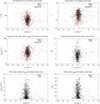 |
Fig. 1. Derived physical parameters for absorption components (Ts, τ, nCNM, Mt, NCNM, and fCNM) depending on turbulent velocity deviations Δv from filament velocities. Data from the GASKAP-H I survey are indicated by black symbols; + in case of FIR/H I filaments and x in case of genuine H I filaments. BIGHICAT data from FIR/H I filaments at latitudes |b|> 10° are included for reference and indicated by red symbols. |
For the determination of volume densities nCNM, we assumed that the CNM is in thermal equilibrium with the associated WNM at a characteristic equilibrium pressure of log(p/k) = 3.58 (Jenkins & Tripp 2011). This applies if the CNM filaments had sufficient time to reach thermal equilibrium, a condition that most probably is valid in magnetically aligned filaments (Paper III, Sect. 7.1). As nCNM ∝ Ts−1, the volume density distribution in Fig. 1 is inverse to the Ts distribution. For a median Ts = 50 K, we obtained a median density of nCNM = 76 cm−3.
To determine the turbulent Mach numbers, we used the relation  (e.g., Heiles & Troland 2003). Here, TD is the Doppler temperature, determined as TD = 121 σem2 from the velocity dispersion σem of the observed GASKAP-H I CNM component in emission. In a turbulent ISM, we have an upper limit to the kinetic temperature TD > Tk2, and for the CNM, we can use the approximation TD > Ts (McClure-Griffiths et al. 2023). In the absence of optical depth measurements, TD is often used to estimate temperatures of the H I gas. From the GASKAP-H I database, we determined an average Mt = 3.4 ± 1.6 for all components but Mt = 3.7 ± 1.6 for those associated with FIR filaments; the latter is consistent with the results from the Millennium Survey by Heiles & Troland (2005). Figure 2 shows the relation between TD and Ts. The huge scatter is obvious, and TD does not measure a temperature, but it is still safe to use TD to derive the nature of a multiphase component. For example, it is valid to assume that filaments with typical Doppler temperatures ⟨TD⟩∼220 K are dominated by the CNM (Clark et al. 2019) or (Kalberla et al. 2016). The GASKAP-H I data, represented in Fig. 2, are important since they provide, for the first time, a large homogeneous database that is useful to observationally relate TD with Ts.
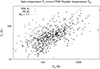 |
Fig. 2. Spin temperatures Ts versus Doppler temperatures TD derived from GASKAP-H I data. A constant slope for Mt = 3.4 is indicated. |
The source distribution, observed by Nguyen et al. (2024), enables the small-scale structure of the CNM to be studied in position-velocity space. For each of the observed absorption positions, we determined the nearest neighbors. Then, we compared pairwise absorption components with the least velocity deviations |Δv|. Similar to Crovisier et al. (1985), we determined relative parameter changes defined as
 (1)
(1)
Here, P can be replaced with Ts, τ, or any of the measured absorption line parameters depending either on separation S in position or displacement in velocity Δv = v1 − v2.
Figure 3 shows, as an example, the relative changes in spin temperature Ts depending on the displacement and velocity spread of the component pairs3. For angular separations of up to 1°, we determined the relative parameter changes ΔTs = 0.23 ± 0.18, Δτ = 0.31 ± 0.22, ΔNCNM = 0.28 ± 0.21, and ΔfCNM = 0.26 ± 0.20. The scatter is large for each of the parameters, but on average the relative changes are moderate.
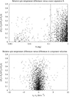 |
Fig. 3. Relative changes ΔTs in spin temperatures Ts. Top: Relative changes ΔTs depending on source separations S. The vertical line indicates the average filament width. Bottom: Relative changes ΔTs depending on velocity differences v1 − v2. |
To gain insight into the nature of the observed velocity fluctuations, we considered the deviations Δv for all pairs of matching absorption components for neighbor positions of up to 20° of separation. Fig. 4 shows a clear trend that Δv increases systematically with separation. A key feature of turbulence is that motions are spatially correlated (Larson 1979). Following Wolfire et al. (2003, Eq. (1)), we used the relation σv(l) = σv(1) lq, where l is the length scale and σv(1) = 1.2 km s−1 is the dispersion at l = 1 pc. In the case of supersonic turbulence, q is expected to be in the range 1/3 ≲ q ≲ 1/2; Larson (1979) found q = 0.37. In Fig. 4, we plot for comparison the solutions for q = 0.37 and q = 0.5, assuming that the CNM is at a distance of 250 pc (Nguyen et al. 2024). Consistent with Heyer et al. (2009), q ∼ 0.5 appears to match the data best over a length scale of four orders of magnitude, with only an insignificant number of outliers.
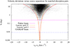 |
Fig. 4. Velocity differences v1 − v2 depending on angular source separation S for matched absorption components. The horizontal lines indicate the Parkes and GASKAP beamwidths. The red and yellow lines display envelopes to the distribution, assuming a turbulent scaling between velocity and length scale (Larson 1979) with exponent q (see text). |
4. Discussion
Sensitive H I absorption data are essential for understanding the physics of the ISM. The recent investigations by Nguyen et al. (2024), which represent the largest Galactic neutral hydrogen H I absorption survey to date, more than double the available absorption lines at high Galactic latitudes. We used the physical parameters derived by these authors and related them to caustics, filamentary structures that have been determined previously from emission line observations in H I and in FIR observations by Planck.
The absorption line detections by Nguyen et al. (2024) probe the CNM, and these lines of sights intersect FIR and H I filaments. Of the positions, 57% are found to be related to common FIR/H I structures with coherent filament velocities. To compare H I and FIR structures, we needed to take sensitivity limitations into account. It was shown in Figs. 8 and 9 of Paper III that only a fraction of the H I filaments can be assigned to FIR structures, but still there is a close relation between FIR and H I. The center velocities of the observed absorption lines share the filament velocities, observed in H I emission, with some fluctuations. These velocity deviations, which we address to turbulent motions, have a dispersion of δvturbHI = 2.48 km s−1 for the whole H I sample, but δvturbFIR = 3.9 km s−1 for FIR filaments. The FIR filaments tend to be more prominent with larger aspect ratios; hence, they show a larger dispersion (Paper III). The FIR/H I filaments tend to have lower mean spin temperatures, TsFIR ∼ 49 K, compared to components that are only associated with H I filaments, TsHI ∼ 67 K. Thus, dusty FIR filaments appear to be colder but more turbulent. All of the GASKAP-H I absorption components are located within caustics. This finding supports our previous conclusions from BIGHICAT data that the FIR/H I filaments originate from dense CNM structures (Paper III).
Cold neutral medium components that are observed in absorption trace the filaments in position-velocity space. For an estimated distance of 250 pc (Nguyen et al. 2024), the typical FIR/H I filament width is 0.63 pc. A GASKAP beam corresponds to a linear size of ∼0.04 pc. For an observed dispersion of Δv ∼ 4 km s−1, the filament crossing time for small-scale CNM structures is typically 0.16 My, which is large in comparison to the expected cooling time of 3 ⋅ 104 y (Jenkins & Tripp 2011). In the case of phase transitions for H I gas with low turbulent deviation velocities, condensations with a high CNM fraction fCNM (Fig. 1) have time to develop.
We considered the question of whether any of the derived CNM parameters, in particular spin temperature Ts, optical depth τ, and CNM fraction fCNM, could depend on the apparent strength of the filamentary structure, as characterized by its eigenvalue −λ−. We find no obvious dependencies (see Fig. A.1 as an example for a deep critical point that is associated with a low optical depth feature). In particular, we found that caustics at a level of λ− ≲ − 5 K deg−2, which is ten times lower than assumed in Paper I, are still significant.
Considering the fluctuations of the derived physical parameters, we found on average only moderate relative changes of 23% to 31% in Ts, τ, or other parameters, independent of source separation or velocity deviation. However, we found indications that the observed dense CNM structures with significant optical depth exist preferentially at filament locations with a low local filament curvature C = 1/R and a large local radius R (see Fig. 5 for fCNM as an example).
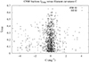 |
Fig. 5. Cold neutral medium fractions fCNM depending on local filament curvatures C. |
Filaments with curvatures of |C|≲1 deg−1 can, as demonstrated by Clark et al. (2014), be straightforwardly analyzed with the Rolling Hough Transform with window diameters 50′≲DW ≲ 125′. For filaments that are aligned with the magnetic field line, a low curvature is expected at positions with an enhanced magnetic field. For a small-scale dynamo, magnetic field strength and curvature are anticorrelated, |B|∝|C|−1/2 (Schekochihin et al. 2004 and St-Onge & Kunz 2018), and the curvature distribution of FIR/H I filaments was found to be characteristic for structures generated by a small-scale dynamo (Paper I). As demonstrated with Fig. 2, these H I filaments that have previously been observed in emission with characteristic Doppler temperatures of TD = 220 K belong to the CNM.
In summary, we conclude that all currently available data from H I absorption line observations at high Galactic latitudes are consistent with the assumption that a major part, if not all, of the CNM is located within magnetically aligned filaments that can be traced on large scales in FIR and in H I emission. These FIR/H I caustics are affected by turbulent velocity perturbations of 3–4 km s−1. The filaments are coherent structures in position-velocity space with well-defined physical properties as CNM in a diffuse multiphase medium.
The GASKAP-H I main survey in full mode, with an integration time 20 times longer than the Pilot II observations considered here, will achieve a ∼4.5 times higher sensitivity.
A few authors therefore denote TD as Tk, max.
In all cases, the pairs are defined as the absorption components with the minimum velocity deviation |v1 − v2|.
For downloads of eigenvalue spectra see https://www.astro.uni-bonn.de/hisurvey/AllSky_gauss/index.php
Acknowledgments
This scientific work uses data obtained from Inyarrimanha Ilgari Bundara / the Murchison Radio-astronomy Observatory. We acknowledge the Wajarri Yamaji People as the Traditional Owners and native title holders of the Observatory site. CSIRO’s ASKAP radio telescope is part of the Australia Telescope National Facility (https://ror.org/05qajvd42). Operation of ASKAP is funded by the Australian Government with support from the National Collaborative Research Infrastructure Strategy. ASKAP uses the resources of the Pawsey Supercomputing Research Centre. Establishment of ASKAP, Inyarrimanha Ilgari Bundara, the CSIRO Murchison Radio-astronomy Observatory and the Pawsey Supercomputing Research Centre are initiatives of the Australian Government, with support from the Government of Western Australia and the Science and Industry Endowment Fund. HI4PI is based on observations with the 100-m telescope of the MPIfR (Max-Planck- Institut für Radioastronomie) at Effelsberg and Murriyang, the Parkes radio telescope, which is part of the Australia Telescope National Facility (https://ror.org/05qajvd42) which is funded by the Australian Government for operation as a National Facility managed by CSIRO. This research has made use of NASA’s Astrophysics Data System. Some of the results in this paper have been derived using the HEALPix package.
References
- Castrigiano, D., & Hayes, S. 2004, Catastrophe Theory, 2nd edn. (CRC Press) [Google Scholar]
- Clark, S. E., & Hensley, B. S. 2019, ApJ, 887, 136 [NASA ADS] [CrossRef] [Google Scholar]
- Clark, S. E., Peek, J. E. G., & Putman, M. E. 2014, ApJ, 789, 82 [NASA ADS] [CrossRef] [Google Scholar]
- Clark, S. E., Peek, J. E. G., & Miville-Deschênes, M.-A. 2019, ApJ, 874, 171 [NASA ADS] [CrossRef] [Google Scholar]
- Crovisier, J., Dickey, J. M., & Kazes, I. 1985, A&A, 146, 223 [NASA ADS] [Google Scholar]
- Heiles, C., & Troland, T. H. 2003, ApJ, 586, 1067 [NASA ADS] [CrossRef] [Google Scholar]
- Heiles, C., & Troland, T. H. 2005, ApJ, 624, 773 [NASA ADS] [CrossRef] [Google Scholar]
- Heyer, M., Krawczyk, C., Duval, J., et al. 2009, ApJ, 699, 1092 [Google Scholar]
- HI4PI Collaboration (Ben Bekhti, N., et al.) 2016, A&A, 594, A116 [NASA ADS] [CrossRef] [EDP Sciences] [Google Scholar]
- Jenkins, E. B., & Tripp, T. M. 2011, ApJ, 734, 65 [NASA ADS] [CrossRef] [Google Scholar]
- Kalberla, P. M. W. 2024, A&A, 683, A36 [NASA ADS] [CrossRef] [EDP Sciences] [Google Scholar]
- Kalberla, P. M. W., & Haud, U. 2015, A&A, 578, A78 [NASA ADS] [CrossRef] [EDP Sciences] [Google Scholar]
- Kalberla, P. M. W., & Haud, U. 2023, A&A, 673, A101 [NASA ADS] [CrossRef] [EDP Sciences] [Google Scholar]
- Kalberla, P. M. W., Kerp, J., Haud, U., et al. 2016, ApJ, 821, 117 [Google Scholar]
- Kalberla, P. M. W., Kerp, J., & Haud, U. 2020, A&A, 639, A26 [EDP Sciences] [Google Scholar]
- Kalberla, P. M. W., Kerp, J., & Haud, U. 2021, A&A, 654, A91 [NASA ADS] [CrossRef] [EDP Sciences] [Google Scholar]
- Larson, R. B. 1979, MNRAS, 186, 479 [NASA ADS] [CrossRef] [Google Scholar]
- Lazarian, A., & Pogosyan, D. 2000, ApJ, 537, 720 [NASA ADS] [CrossRef] [Google Scholar]
- Lazarian, A., & Yuen, K. H. 2018, ApJ, 853, 96 [NASA ADS] [CrossRef] [Google Scholar]
- Lei, M., & Clark, S. E. 2024, ApJ, 972, 66 [Google Scholar]
- McClure-Griffiths, N. M., Pisano, D. J., Calabretta, M. R., et al. 2009, ApJS, 181, 398 [NASA ADS] [CrossRef] [Google Scholar]
- McClure-Griffiths, N. M., Stanimirović, S., & Rybarczyk, D. R. 2023, ARA&A, 61, 19 [NASA ADS] [CrossRef] [Google Scholar]
- Murray, C. E., Peek, J. E. G., & Kim, C.-G. 2020, ApJ, 899, 15 [CrossRef] [Google Scholar]
- Nguyen, H., McClure-Griffiths, N. M., Dempsey, J., et al. 2024, MNRAS, 534, 3478 [NASA ADS] [CrossRef] [Google Scholar]
- Peek, J. E. G., & Clark, S. E. 2019, ApJ, 886, L13 [NASA ADS] [CrossRef] [Google Scholar]
- Planck Collaboration Int. LVII. 2020, A&A, 643, A42 [NASA ADS] [CrossRef] [EDP Sciences] [Google Scholar]
- Saury, E., Miville-Deschênes, M.-A., Hennebelle, P., et al. 2014, A&A, 567, A16 [NASA ADS] [CrossRef] [EDP Sciences] [Google Scholar]
- Schekochihin, A. A., Cowley, S. C., Taylor, S. F., et al. 2004, ApJ, 612, 276 [NASA ADS] [CrossRef] [Google Scholar]
- St-Onge, D. A., & Kunz, M. W. 2018, ApJ, 863, L25 [CrossRef] [Google Scholar]
- Winkel, B., Kerp, J., Flöer, L., et al. 2016, A&A, 585, A41 [NASA ADS] [CrossRef] [EDP Sciences] [Google Scholar]
- Wolfire, M. G., McKee, C. F., Hollenbach, D., et al. 2003, ApJ, 587, 278 [Google Scholar]
- Yuen, K. H., Ho, K. W., & Lazarian, A. 2021, ApJ, 910, 161 [NASA ADS] [CrossRef] [Google Scholar]
Appendix A: Eigenvalues
Eigenvalues λ− are determined from a Hessian analysis of the HI4PI survey according to Kalberla2024, Eqs. (1) and (2). Caustics can be identified as critical points with λ− < 0. These eigenvalues have been determined all sky for velocities −50 < vLSR < 50 km s−1. To distinguish H I and FIR caustics, orientation angles Θ according to (Kalberla2024, Eq. (3)), were used. At a given position, the line of sight may intersect several H I caustics at different velocities but only a single FIR caustic can be detectable. In addition to eigenvalues, the associated orientation angles (derived from eigenvectors) are used to match FIR and H I filaments. The H I caustic with the best alignment, hence the minimum of |ΘFIR − ΘHI|, defines the velocity of the FIR filament. The uncertainties in matching orientation angles of FIR and H I filaments are below 3°, see (Kalberla2021, Table 1).
A.1. Eigenvalue spectra
Figure A.1 shows two examples for the relation between eigenvalues λ− and H I absorption. On top of Fig. A.1 the source J032548-735326 is shown. The brightness temperatures, observed with HI4PI and GASKAP-H I close to the source, are plotted in blue and magenta. The eigenvalues λ− (black) indicate five H I caustics (red), one of them is associated with an FIR caustic. From the GASKAP-H I pilot project observations, two significant H I absorption lines (yellow) can be identified; a third potential absorption feature (arrow) is observed below the detection threshold. These absorption features are associated with caustics, for more observational details see Nguyen et al.(2024, Fig. 8).
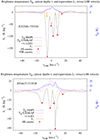 |
Fig. A.1. Hessian eigenvalues λ− (black) related to observed brightness temperatures at the nearest position. HI4PI data are indicated in blue and GASKAP-H I data in magenta. Critical points λ− < 0 are marked in red. Top: for the source J032548-735326 two absorption components (orange, scaled by a factor of 200) are indicated with an additional feature below the detection limit (arrow). For observational details see Fig. 8 of Nguyen et al. (2024). Bottom: the source J054427-715528 has a single absorption component (orange, scaled by a factor of 40). For observational details see Fig. 3 of Nguyen et al. (2024). |
The source J054427-715528, shown at the bottom of Fig. A.1, has five H I caustics that are not related to an FIR filament. Only one of these caustics is associated with a detected absorption line. However, we observed significant fluctuations at velocities of two of the caustics when comparing the HI4PI and GASKAP-H I brightness temperature profiles close to the source position. The HI4PI and GASKAP-H I beamwidths (14 5 and 30″, respectively) are largely different, hence these fluctuations indicate small scale structure that is usually addressed to CNM. More observational details for the source J054427-715528 are given in Fig. 3 of Nguyen et al. (2024).
The example eigenvalue spectra in Fig. A.1 have been chosen to allow a comparison with published absorption spectra. Depending on the H I emission distribution, the λ− spectra can have far more complex shapes. For the data analysis it is only necessary to determine critical points with λ− < 0, marked in red in the examples4.
A.2. Turbulent velocity dispersions
In Kalberla2021 it was shown that FIR/H I filaments are shaped by a small-scale turbulent dynamo. In such a case the filament curvatures show a characteristic pattern (Schekochihin et al. 2004 and St-Onge & Kunz 2018). A succession of random velocity shears stretches the magnetic field and leads on the average to its growth to dynamical strengths. This process leads to filamentary structures of near-constant velocity along magnetic lines of force. Both, characteristic curvatures and near-constant velocities along filaments, are observed Kalberla2021. Numerical studies of the condensation of the WNM into CNM structures under the effect of turbulence and thermal instability by Saury et al. (2014) indicate that the velocity field of the CNM reflects the velocity dispersion of the WNM. These authors estimate a CNM cloud-to-cloud velocity dispersion to 5.9 km s−1 from observations and find about 3 km s−1 in simulations.
In case of phase transitions within a turbulent medium that is affected by a dynamo it is expected that the near-constant velocity field along magnetic lines of force is locally perturbed. Assuming the CNM aligned preferential along the filaments, a CNM cloud-to-cloud velocity dispersion in the order of 3 to 6 km s−1 is expected along the filaments (Kalberla2024, Sect. 7). In this context it is also reasonable to assume turbulence along the line of sight and to define a turbulent velocity deviation Δv between filament and absorption component. The GASKAP and GASS beams are very different, thus Δv measure differences between pencil beam of 30″and the effective beam of the Hessian operator (5x5 pixels, or ∼18′ for an nside = 1024 HEALPix grid) which is close to the GASS beam. Thus, Δv measures in this case the velocity deviations of absorption components relative to the filament body.
In Fig. A.2 we display dependencies between caustic eigenvalues −λ− and turbulent velocity deviations Δv = vabs − vfilHI and Δv = vabs − vfilFIR for H I and FIR filaments respectively. Comparing H I and FIR, we need to take different survey sensitivities into account (e.g., Kalberla et al. 2016, Fig. 4); H I and FIR eigenvalues need to be treated separately. Figure A.2 shows the GASKAP-H I eigenvalues as function of the associated turbulent velocity deviations Δv for FIR and H I surveys independently.
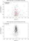 |
Fig. A.2. Hessian eigenvalues λ− for absorption components depending on turbulent velocity deviations Δv from filament velocities. Top: GASKAP-H I data for FIR filaments, including BIGHICAT results. Bottom: GASKAP-H I data for H I filaments, no BIGHICAT data in this case. |
The upper part of Fig. A.2 considers FIR eigenvalues −λ− depending on turbulent velocity deviations Δv. For comparison with Fig. 5 of Kalberla2024 we include previous results from BIGHICAT, 97 components for galactic latitudes |b|> 10°. For GASKAP FIR we determine a dispersion of δvturb = 3.9 km s−1, consistent with δvturb = 3.7 km s−1 in case of BIGHICAT sources (red). This compares well to δvturb = 3.8 ± 0.1 km s−1 for the velocity dispersion along the FIR/H I filaments observed in the plane of the sky Kalberla2024.
For turbulent velocity deviations Δv in case of H I filaments (lower part of Fig. A.2) we determine an average vav = 6. 10−2 km s−1 with a dispersion of δvturb = 2.48 km s−1. This result confirms the visual impression that H I filaments have significant lower turbulent velocity deviations than FIR dominated structures.
All Figures
|
Fig. 1. Derived physical parameters for absorption components (Ts, τ, nCNM, Mt, NCNM, and fCNM) depending on turbulent velocity deviations Δv from filament velocities. Data from the GASKAP-H I survey are indicated by black symbols; + in case of FIR/H I filaments and x in case of genuine H I filaments. BIGHICAT data from FIR/H I filaments at latitudes |b|> 10° are included for reference and indicated by red symbols. |
| In the text | |
|
Fig. 2. Spin temperatures Ts versus Doppler temperatures TD derived from GASKAP-H I data. A constant slope for Mt = 3.4 is indicated. |
| In the text | |
|
Fig. 3. Relative changes ΔTs in spin temperatures Ts. Top: Relative changes ΔTs depending on source separations S. The vertical line indicates the average filament width. Bottom: Relative changes ΔTs depending on velocity differences v1 − v2. |
| In the text | |
|
Fig. 4. Velocity differences v1 − v2 depending on angular source separation S for matched absorption components. The horizontal lines indicate the Parkes and GASKAP beamwidths. The red and yellow lines display envelopes to the distribution, assuming a turbulent scaling between velocity and length scale (Larson 1979) with exponent q (see text). |
| In the text | |
|
Fig. 5. Cold neutral medium fractions fCNM depending on local filament curvatures C. |
| In the text | |
|
Fig. A.1. Hessian eigenvalues λ− (black) related to observed brightness temperatures at the nearest position. HI4PI data are indicated in blue and GASKAP-H I data in magenta. Critical points λ− < 0 are marked in red. Top: for the source J032548-735326 two absorption components (orange, scaled by a factor of 200) are indicated with an additional feature below the detection limit (arrow). For observational details see Fig. 8 of Nguyen et al. (2024). Bottom: the source J054427-715528 has a single absorption component (orange, scaled by a factor of 40). For observational details see Fig. 3 of Nguyen et al. (2024). |
| In the text | |
|
Fig. A.2. Hessian eigenvalues λ− for absorption components depending on turbulent velocity deviations Δv from filament velocities. Top: GASKAP-H I data for FIR filaments, including BIGHICAT results. Bottom: GASKAP-H I data for H I filaments, no BIGHICAT data in this case. |
| In the text | |
Current usage metrics show cumulative count of Article Views (full-text article views including HTML views, PDF and ePub downloads, according to the available data) and Abstracts Views on Vision4Press platform.
Data correspond to usage on the plateform after 2015. The current usage metrics is available 48-96 hours after online publication and is updated daily on week days.
Initial download of the metrics may take a while.