| Issue |
A&A
Volume 683, March 2024
|
|
|---|---|---|
| Article Number | A36 | |
| Number of page(s) | 16 | |
| Section | Interstellar and circumstellar matter | |
| DOI | https://doi.org/10.1051/0004-6361/202348056 | |
| Published online | 04 March 2024 | |
Caustics and velocity caustics in the diffuse interstellar medium at high Galactic latitudes
Argelander-Institut für Astronomie, University of Bonn,
Auf dem Hügel 71,
53121
Bonn,
Germany
e-mail: This email address is being protected from spambots. You need JavaScript enabled to view it.
Received:
24
September
2023
Accepted:
8
December
2023
Abstract
Context. The far-infrared (FIR) distribution at high Galactic latitudes, observed with Planck, is filamentary with coherent structures in polarization. These structures are also closely related to H I filaments with coherent velocity structures. There is a long-standing debate about the physical nature of these structures. They are considered either as velocity caustics, fluctuations engraved by the turbulent velocity field or as cold three-dimensional density structures in the interstellar medium (ISM).
Aims. We discuss different approaches to data analysis and interpretation in order to work out the differences.
Methods. We considered mathematical preliminaries for the derivation of caustics that characterize filamentary structures in the ISM. Using the Hessian operator, we traced individual FIR filamentary structures in H I from channel maps as observed and alternatively from data that are provided by the velocity decomposition algorithm (VDA). VDA is claimed to separate velocity caustics from density effects.
Results. Based on the strict mathematical definition, the so-called velocity caustics are not actually caustics. These VDA data products may contain caustics in the same way as the original H I observations. Caustics derived by a Hessian analysis of both databases are nearly identical with a correlation coefficient of 98%. However, the VDA algorithm leads to a 30% increase in the alignment uncertainties when fitting FIR/H I orientation angles. Thus, the VDA velocity crowding concept fails to explain the alignment of FIR/H I filaments at |b| > 20°. We used H I absorption data to constrain the physical nature of FIR/H I filaments and determine spin temperatures and volume densities of FIR/H I filaments. H I filaments exist as cold neutral medium (CNM) structures; outside the filaments no CNM absorption is detectable.
Conclusions. The CNM in the diffuse ISM is exclusively located in filaments with FIR counterparts. These filaments at high Galactic latitudes exist as cold density structures; velocity crowding effects are negligible.
Key words: ISM: clouds / ISM: structure / dust, extinction / turbulence / magnetic fields / magnetohydrodynamics (MHD)
© The Authors 2024
 Open Access article, published by EDP Sciences, under the terms of the Creative Commons Attribution License (https://creativecommons.org/licenses/by/4.0), which permits unrestricted use, distribution, and reproduction in any medium, provided the original work is properly cited.
This article is published in open access under the Subscribe to Open model. This email address is being protected from spambots. You need JavaScript enabled to view it. to support open access publication.
1 Introduction
Take a teacup. At the bottom of this cup you can observe a caustic, the image of the Sun focused typically into two bright curves with a central peak. Caustics can also be generated by refraction, like a rainbow or the wiggling patterns at the bottom of a swimming pool. Simple structures of this kind can be explained by ray tracing1. Gravitational lensing and microlensing events are examples of more complex cases. The shapes of these caustics depend on the source distribution and the intervening matter (e.g., Blandford & Narayan 1992). Caustics are also found in topological structures of the cosmic web, such as voids, peaks, walls, and filaments (e.g., Bond et al. 1996). A general formalism for caustics that also applies to such complex structures has been given recently by Feldbrugge et al. (2018).
For the interpretation of caustics it is in general necessary to know some details of the physics of the imaging system as well as its geometry. This implies that some initial model assumptions are needed. Consent about model conditions is not always granted; different groups may advocate controversial models, and we are then faced with a diversity of possible interpretations. In this paper we discuss such a case, the interpretations of observed caustics in the diffuse interstellar medium. Prominent filamentary structures, observable with Planck at 857 GHz or 353 GHz (Planck Collaboration Int. XXXII. 2016; Planck Collaboration Int. XXXV. 2016; Planck Collaboration Int. XXXVIII 2016), are found to be well aligned with the ambient magnetic field in the diffuse interstellar medium (ISM). These small-scale structures caused by emission from dust in the far-infrared (FIR) are well aligned with small-scale H I structures and the discussion is about the nature of the observed intensity enhancements in H I channel maps.
One the one hand, these filamentary structures have been interpreted as caustics originating from real physical structures, coherent H I fibers with local density enhancements in position-velocity space. The ISM is understood as a multiphase medium with a diffuse warm neutral medium (WNM) in pressure equilibrium with the embedded cold neutral medium (CNM; e.g., Wolfire et al. 2003). This CNM, observed with a characteristic narrow velocity distribution, is filamentary and associated with cold dust, stretched out along the magnetic field lines (e.g., Clark et al. 2014, 2019; Kalberla et al. 2016, or Peek & Clark 2019).
Counterarguments are based on Lazarian & Pogosyan (2000). The observed filaments accordingly indicate velocity caustics caused by turbulent velocity fluctuations. The observed intensity enhancements in channel maps with small velocity widths originate in this approach from nonlinear density fields that are transformed by coherent turbulent velocities. The emission is generated in different volume elements, separated along the line of sight. Intensity enhancements are thus generated by velocity crowding. H I intensity enhancement may therefore not be interpreted as real coherent density structures, but reflect the properties of random turbulent fields. Such structures are referred to as velocity caustics
In this paper, we discuss the two opposing positions. We focus on phenomena that lead to observable caustics in the diffuse interstellar medium. The scientific community needs to distinguish between the two different approaches that are described in almost identical terms, caustics and velocity caustics. In the first case we have generic caustics (καυσrτικóζ), as introduced in the first paragraph. These caustics are deterministic. A particular source distribution generates a characteristic image, and a trace-back is possible. In the second case of velocity caustics, intensity structures originate from turbulent velocity fluctuations. The statistical nature of this process does not allow conclusions about distinct source properties like temperature and volume density of the H I.
This paper is structured as follows. We first consider in Sect. 2 the morphology of generic caustics and the mathematical approaches that define such caustics. Next we discuss in Sect. 3 velocity caustics in context with the velocity channel analysis (VCA), proposed by Lazarian & Pogosyan (2000) and the derived velocity decomposition algorithm (VDA) by Yuen et al. (2021). In Sect. 4, we calculate the proposed VDA velocity and density contributions, and use the Hessian operator to determine VDA eigenvectors and orientation angles that are then compared with previous results from Kalberla et al. (2021, hereafter Paper I). The numerical results are discussed in Sect. 5; H I power spectra are discussed in Sect. 6. The physical conditions in caustics are considered in Sect. 7. We demonstrate that FIR/H I filaments are unambiguously related to the CNM and demonstrate the differences between velocity slicing and velocity tracing. After a summary in Sect. 8, we conclude that FIR/H I filaments can be traced as small-scale structures in position, associated with coherent structures in velocity with narrow linewidths. FIR/H I caustics are density structures in the positionvelocity space.
2 Caustics: A morphological approach
Caustics are considered by mathematicians as part of the theory of local singularities of smooth morphisms; physicists are more interested in the stability of natural systems. In this context we start with a brief description of the mathematical background and methods that are useful for the determination and analysis of caustics.
2.1 Caustics as Morse complexes
Caustics are defined by their particular topology, and it is challenging to use a morphology-based data analysis to derive physical properties of observed intensity structures. The mathematical framework for a treatment of caustics is based on investigations by Thom (1975) and Arnold et al. (1985). Caustics are usually considered in the more general framework of catastrophe theory2. A recent rigorous treatment of the mathematical background can be found in Castrigiano & Hayes (2004).
Caustics in smooth differentiable maps are related to critical points, positions where the derivative of the investigated distribution function is zero. In 2D maps such positions identify minima, saddle points, and maxima. These are basins, passes, and peaks if we take mountain shapes as examples. These formations are usually structurally stable, and this is the property of generic critical points, also called Morse critical points, that can locally be approximated by quadratic functions. These points need to be nondegenerate, the determinant of the Hessian (the product of the eigenvalues) has to be nonzero. Thus, for our 2D application, structurally stable critical points are characterized locally by x2 + y2 (local minima), x2 − y2 or y2 − x2 (saddles), and −x2 − y2 (local maxima).
Caustics in more than two dimensions are far more complex. Structure analyses of the cosmic web need to take these general cases into account and have recently been discussed by Sousbie (2011), Sousbie et al. (2011), Feldbrugge et al. (2018, 2019)3. Important for our 2D application is that generic caustics on the plane can only exist along A3 caustics, as classified by Arnold, or cusps, which is the notation used by Thom (see Sect. 21.3, corollary 3 in Arnold et al. 1985). In general, the A3 caustics characterize structures that are commonly labeled as filaments or fibers.
Filaments in the ISM have been described by Schisano et al. (2014) as elongated regions with a higher brightness contrast with respect to its surrounding. It is important that visual perceptions of this kind can be (and need to be) unambiguously verified as caustics. Such regions represent what is considered in the sense of a general morphological approach as descending manifolds, passes including connected peaks. Structures of this kind, A3 caustics, can rigorously be extracted by using a Hessian-based filament identification scheme with negative eigenvalues. Alternatively to the Hessian matrix, different methods can be applied. The rolling Hough transform (RHT, Clark et al. 2014) and FILFINDER (Koch & Rosolowsky 2015) have been shown by Soler et al. (2020) to lead to equivalent results.
Formally, the set of all descending manifolds is usually referred to as the Morse complex (Sousbie 2011, definitions 2.4 and 2.5). Filamentary structures can be determined as surfaces of manifolds associated with critical points of order one (saddles) where the Hessian matrix has everywhere exactly one negative eigenvalue (described also as Morse index one). A peak is of order two4. Peaks are isolated and are always connected to passes. Considering these peaks as parts of filaments (otherwise peaks would disrupt filaments) leads to the constraint that for filaments the Morse index must be at least one.
As discussed in Sect. 4, a number of publications since the year 2000 characterize filamentary structures in the ISM as velocity caustics in a rather unsharp and ambiguous way. This is in conflict with the original definition of caustics by Thom (1975) and Arnold et al. (1985), and for the sake of clarity in the following, in most cases we use the term filaments to describe A3 caustics that are characterized by descending manifolds with Morse indices of one or two. Velocity caustics, caused by velocity crowding, have a filamentary appearance, but may not be considered to originate from homogeneous fibers, theads, or filaments.
2.2 The Hessian operator as applied to FIR and HI data
Morse complexes can best be identified with the Hessian matrix H, which is based on partial derivatives of the intensity distribution. This method was used for the first time by Polychroni et al. (2013) for the identification of filamentary structures in Orion A. Planck Collaboration Int. XXXII. (2016) used the Hessian matrix to study the relative orientation between the magnetic field and structures traced by interstellar dust. A recent application of this method to filamentary structures in the Galactic plane is presented in Soler et al. (2022).
In Paper I and Kalberla & Haud (2023, hereafter Paper II) high Galactic latitude structures in FIR and H I data were analyzed. Here we briefly summarize this approach. The Hessian matrix is defined as
 (1)
(1)
Here x and y refer to the true angles in longitude and latitude. The second-order partial derivatives are Hxx = ∂2I/∂x2, Hxy = ∂2I/∂x∂y, Hyx = ∂2I/∂y∂x, and Hyy = ∂2I/∂y2.
The eigenvalues of H,
 (2)
(2)
describe the local curvature of the data (H I and FIR as described in Paper II). Eigenvalues λ− < 0 K/deg−2 with the associated eigenvectors are in direction of least curvature and indicate filamentary structures, passes, or ridges. We use negative thresholds for FIR and H I to identify only significant descending manifolds, hence caustics. The local orientation of filamentary structures relative to the Galactic plane (defined by the eigenvectors) is given by the angle
![Mathematical equation: $\theta = {1 \over 2}\arctan \left[ {{{{H_{xy}} + {H_{yx}}} \over {{H_{xx}} - {H_{yy}}}}} \right],$](/articles/aa/full_html/2024/03/aa48056-23/aa48056-23-eq3.png) (3)
(3)
in analogy to the relation
 (4)
(4)
from polarimetric observations that provide the Stokes parameters U and Q.
The Hessian analysis, including the determination of local orientation angles along the filaments, was applied in Paper I and Paper II to Planck FIR data at 857 GHz. Also considered were HI4PI H I observations (HI4PI Collaboration et al. 2016), combining data from the Galactic All Sky Survey (GASS; Kalberla & Haud 2015), measured with the Parkes radio telescope and the Effelsberg-Bonn H I Survey (EBHIS; Winkel et al. 2016) with data from the 100 m telescope.
The Hessian operator was applied to Planck 857 GHz FIR data with a threshold λ− < −1.5 K deg−2 to ensure the significance of the eigenvalues. This procedure defines an ensemble of isolated FIR filaments. In the next step this analysis was repeated for all H I channels, this time with an eigenvalue threshold λ− < −50 K deg−2. These limits take different sensitivities and intensity scaling in FIR and H I into account; we note that the applied thresholds are related to observed intensities due to the constant multiple rule for derivatives. Each of the FIR manifolds is found to be associated in H I with a distribution of filaments in velocity space (represented by channel maps) that approximately fit local shapes of the FIR structures. Orientation angles θ were used to resolve the velocity ambiguities by searching for a velocity-space alignment of H I structures and orientation angles with the FIR emission.
Each individual FIR position within each of the descending manifolds was compared with each channel of the derived H I manifolds with the aim of finding the velocity with the best match for the local orientation angle θ. Best fit results, on average accurate to σθ = 4°.1, were found for narrow velocity channels with the original instrumental resolution at high Galactic latitudes, see Paper I. These morphologically derived velocities define the velocity field of the FIR filaments. Radial velocities along individual filaments were found to be well defined and coherent with an average random scatter of ∆υLSR = 5.24 km s−1 along the filaments that was interpreted in Paper II as internal turbulent motions of the filaments.
In summary, the Hessian operator was used in Paper I to identify Morse complexes, filaments with common properties for FIR, and H I. Along these filaments FIR and H I share common orientation angles at well-defined coherent H I velocities. Known FIR distances allow volume densities to be determined from observed column densities. The Morse complexes can straightforwardly be interpreted as cold density filaments (see Paper II). Minkowski functionals were found useful to derive aspect ratios and filamentarity of the FIR/H I filaments.
3 Probing the velocity channel analysis
Velocity channel analysis (VCA, Lazarian & Pogosyan 2000) deals with emission spectra in individual velocity slices (channel maps) and derives dependences on the statistics of turbulent velocity and density fields by varying the slice thickness. Here we explain briefly the VCA preliminaries.
3.1 Velocity channel analysis and velocity caustics
H I and molecular line observations are usually organized in position-position-velocity (PPV) data cubes. Channel maps at constant velocities measure line intensities that depend on the physical conditions of the gas at a particular observed radial velocity. The derived parameters are affected by turbulent velocity fluctuations along the line of sight. Additional fluctuations in density are expected. The problem of disentangling velocity and density fluctuations was first addressed in Lazarian & Pogosyan (2000), and subsequently by Lazarian & Pogosyan (2004, 2006, 2008). These authors represent the PPV correlation function as a sum of two uncorrelated terms that depend for each velocity channel either on fluctuations of density or velocity. Accordingly, narrow velocity slices are supposed to be dominated by velocity perturbations and broad slices in the limit are dominated by column density effects. VCA aims in this way to disentangle velocity and density statistics. The claim after these investigations is that structures observed in narrow velocity intervals are caused predominantly by velocity caustics.
Generic caustics are associated with singularities of gradient maps. The most convenient way to search for caustics in 2D is the use of a Hessian-based filament identification scheme. Velocity caustics, generated by velocity crowding, were claimed to have been found in observations and magnetohydrodynam-ics (MHD) simulations by a number of authors (e.g., Esquivel et al. 2003, Chepurnov & Lazarian 2009, Padoan et al. 2009, Lazarian & Yuen 2018, and Ho & Lazarian 2023). However, none of these publications provides a rigorous identification of structures as generic caustics or parts of Morse complexes in the sense of Sect. 2.1 or as described by Thom (1975) and Arnold et al. (1985). In many cases numerical simulations ignore the thermal broadening of the lines that tends to wash out velocity fluctuations (see Clark et al. 2019, Sect. 3.1). Structures that are visible in simulated PPV maps in these cases are not representative for observed PPV maps.
3.2 Definition of the velocity decomposition algorithm
Following the theory by Lazarian & Pogosyan (2000), Yuen et al. (2021) developed a method for decomposing an observed PPV data cube into two separate cubes that are supposed to contain independently the turbulent velocity and density information. The decomposition is based on the postulate that in case of MHD turbulence the density and the velocity fluctuations are statistically uncorrelated. Using VDA notations this is formulated as p = pυ + pd with 〈pυpd〉 = 0, for an ensemble average indicated by 〈…〉. The observed channel map5 p is decomposed in its velocity contribution Pv and density part Pd according to
 (5)
(5)
with I = ∫p(υ)dυ the total H I intensity (or column density) along the line of sight and  . The necessary condition is that the velocity width ∆υ of the PPV channel map is small in comparison to the effective velocity width of the observed H I gas. To relate this condition to the analysis in Paper I we recall that ∆υ = 1 km s−1 was used there. Typical cold H I structures have a velocity width of 3 km s−1, and thus H I is well resolved. VDA velocity fluctuations are noticeable only in narrow velocity intervals, but vanish if velocity slices get thicker; pυ = 0 for ∆υ → ∞. Per the definition, VDA density fluctuations scale as pd ∝ I, in particular for low sonic Mach numbers Ms ≪ 1 (Yuen et al. 2021, Sect. 3).
It is important to realize that Eq. (5) represents a decomposition of velocity and density fluctuations (positive or negative deviations from the mean), while the observed H I channel maps p = pυ + pd are density-weighted emission profiles. The differences between the two approaches are explained in Fig. 2 of Yuen et al. (2021). VDA densities pd, although they are denoted as densities, are not to be confused with volume densities. This can be seen from Eq. (5), where pv and pd have the same units as p from observations. The brightness temperatures TB in K averages over the width of the velocity channel in km s−1. Volume densities demand a definition of the volume that is occupied by the H I (or modeling an object considered as a cloud). This definition is not part of the VCA or VDA concept. Volume densities in the presence of a dominating velocity crowding effect are in this context undefined.
According to Yuen et al. (2021), the term pv in Eq. (5) represents the velocity contribution to velocity channels and is referred to as (or defined as) the velocity caustics contribution. Although they are called velocity caustics, pυ is not the velocity field; it can be seen only as a proxy for the part of the data that are (according to VCA/VDA) affected by the velocity field. These velocity caustics pυ are not to be confused with caustics as defined by Thom (1975) or Arnold et al. (1985). To avoid any conflicts with caustics that are defined as manifolds in 2D, for pυ we use in the following the notation VDA velocity caustics. The observed data p, as well as the contributions pυ or pd may contain manifolds that represent Morse complexes, but each p, pv, or pd velocity slice on its own represents no more than a smooth differentiable map that needs to be analyzed for the presence of supposed caustics before further conclusions can be drawn. Such an analysis is not part of VDA. VCA also does not attempt any morphological decomposition.
4 Hessian analysis of the VDA databases pv and pd
Following Eq. (5), we generate pυ and pd for the observed p database used in Paper I. We repeat the complete Hessian analysis described in Sect. 2 of Paper I independently for VDA derived velocity pυ and density pd structures without modifying any of the program parameters. In the following we discuss the properties derived from Hessian eigenvalues and eigenvectors independently.
4.1 Correlations of λ− eigenvalues in p and pv
Inspecting derived eigenvalues for λ− in p and pυ visually, we find a close agreement between the two distributions. The correlation between the A and B distributions can, according to Yuen et al. (2021), be best verified by using the normalized covariance coefficient
 (6)
(6)
to characterize correlations between the two 2D maps A and B; here we use the same notations as Yuen et al. (2021). This measure, also known as Pearson product-moment correlation coefficient, is scale-invariant and results in NCC(A, B) ∈ [−1, 1]. The case NCC(A, B) = 0 implies that the two maps are statistically uncorrelated. A perfect correlation requires that NCC(A, B) = ±1; the sign reflects the slope of the linear regression that can be fitted in this case.
The correlation coefficients NCC(λ−(p), λ−(pυ)) for the eigenvalue distributions at all velocity channels −50 < υLSR < 50 km s−1 are shown in Fig. 1. The best correlations with NCC(λ−(p), λ−(pυ)) ≳ 0.98 are found at latitudes |b| > 20° in the case of filamentary structures constrained in H I by λ− < −50 K deg−2. This is the same condition as used in Paper to ensure that H I filaments are unaffected by observational uncertainties. Unconstrained λ−(p) and λ−(pυ) eigenvalue distributions at high latitudes show only a perfect correlation for |υLSR| ≲ 8 km s−1; this is the velocity range with dominant CNM filaments (see Fig. 11 in Paper I). The λ−(p) and λ−(pυ) eigenvalue distributions at low Galactic latitudes suffer from confusion (Paper II, Sect. 3.1) and the correlation NCC(λ−(p), λ−(pυ)) degrades significantly, whether they are constrained or not.
After discussing the general correlation analysis on Galactic scales we display on top of Fig. 2 an example for the eigenvalue distribution λ−(pυ) together with deviations λ−(pυ) − λ−(p). Minor deviations are visible, they reflect the result that the eigenvalues λ− for p and pυ at high Galactic latitudes are highly similar. At the bottom of Fig. 2 we display for comparison the velocity field of the FIR filaments derived from pυ, together with deviations from the velocity field published in Paper I.
The Hessian analysis of the VDA velocity term pυ, using exactly the same procedures as in Paper I, recovers in 97% of all case positions in the Morse complexes that are identical with the positions of the filamentary structures found in Paper I. Less than half (43%) of the previously derived filament positions have identical VDA filament velocities but for 53% of them the differences are below 1 km s−1. Allowing uncertainties of ∆υ < 6 km s−1 for the filament velocities (see Sect. 2.6 of Paper I), we obtain compatible velocities for 68% of all filament positions. A close inspection of the lower part of Fig. 2 reveals that positions with significant differences in the derived velocities are located predominantly on the filament outskirts. In comparison to the filament centers, these positions have a lower signal-to-noise ratio (S/N). We also note an increase in the velocity uncertainties toward the Galactic plane, explainable with increasing confusion due to the increasing complexity of the H I emission.
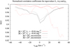 |
Fig. 1 Normalized correlation coefficients for eigenvalues in observed intensity p and VDA velocity caustics pυ according to Eq. (5) at high and low Galactic latitudes. Data constrained by λ− < −50 K deg−2 (used in Paper I to compare H I with FIR filaments) and unconstrained eigenvalues are distinguished. |
4.2 Orientation angle alignments between  , θp, and θFIR
In the previous subsection we considered agreements in eigenvalues λ−. In the following, we take the eigenvectors into account. These determine the local orientation of filamentary structures and are conveniently parameterized by the angle θ according to Eq. (3). We complete the comparison between filamentary structures in pυ and p with a summary of orientation angle alignments in Table 1 and Fig. 3. To allow an easy comparison, we replicate the previously derived best fit entries from Fig. 3 and Table 1 of Paper I.
For a detailed definition of the different alignment measures in Table 1 we refer to Paper I. Here we provide only a brief description. To measure the angular alignments between two data sets we calculate first the angular difference between the orientation angles Θ1 and Θ2 at each position:
![Mathematical equation: $\delta \theta = {1 \over 2}\arctan \left[ {{{\sin \left( {2{\theta _1}} \right)\cos \left( {2{\theta _2}} \right) - \cos \left( {2{\theta _1}} \right)\sin \left( {2{\theta _2}} \right)} \over {\cos \left( {2{\theta _1}} \right)\cos \left( {2{\theta _2}} \right) + \sin \left( {2{\theta _1}} \right)\sin \left( {2{\theta _2}} \right)}}} \right]{\rm{.}}$](/articles/aa/full_html/2024/03/aa48056-23/aa48056-23-eq9.png) (7)
(7)
The width of the resulting δθ distribution, shown in Fig. 3, can be measured by fitting either a Gaussian or a Voigt function; the Voigt function approximates noisy data best. Table 1 lists the fitted δθ dispersions σGauss and σVoigt. The mean degree of alignment, ξ = 〈cosϕ〉, can be defined for ϕ = 2δθ (Clark & Hensley 2019). A different metric, the projected Rayleigh statistic (PRS), was calculated according to Jow et al. (2018),
 (8)
(8)
and the uncertainty of this measure is estimated as
 (9)
(9)
Equation (8) approximates the more general Eq. (4) of Soler et al. (2022) in the case of constant statistical weights. This is justified to a high degree for the all-sky surveys in FIR and H I that we are using here.
The distributions of angular alignment deviations according to Eq. (5) of Paper I between orientation angles of FIR filaments and H I structures are very similar if we use the VDA pv in place of observed H I brightness temperatures p. The best fit result for the velocity width of the slices used, presented in Sect. 2 of Paper I, remains valid and is obtained when using H I channel maps with a velocity width of ∆υ = 1 km s−1. Filamentary structures in the VDA velocity caustics pυ have a ~30% broader δθ distribution compared to the best fit distribution obtained from observed H I channel maps p (see the widths of the distributions in Fig. 3 and the dispersions σGauss and σVoigt in Table 1). The angular alignment deviations for the VDA density distribution pd (Fig. 3 bottom) are unacceptably large, and the filling factors f = 0.04 in Table 1 are extremely low. The sky contains a negligible amount of filaments from the VDA pd distribution. The VDA densities pd are derived from scaled H I column densities according to Eq. (5), and we found already in Sect. 2 of Paper I that integrating the H I distribution does not lead to an improvement in the angular alignment measures.
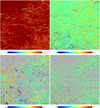 |
Fig. 2 Display of example data in gnomonic projection. The field center is at l = 160°, b = 30°, the field size 27°.7. Top left: eigenvalues λ_(pυ) of VDA velocity caustics pυ at υLSR = 0 km s−1. Top right: deviations λ_(pυ) − λ_(p) between eigenvalues from VDA velocity caustics pυ and observed intensities p. Bottom left: velocities υLSR(pυ) of filamentary FIR structures in case of H I filaments derived for VDA velocity caustics pυ. Bottom right: deviations υLSR(pυ) − υLSR(p) from the velocity field υLSR(p) shown in Fig. 6 of Paper I. |
5 Evaluation: caustics in pv contra p
After an introduction to morphological concepts that define caustics according to Thom (1975) or Arnold et al. (1985), we discussed methods to derive caustics. We also introduced VDA, derived the databases according to the VDA technique and calculated caustics of the VDA databases. These results were compared with caustics from H I data in conventional PPV databases. In both cases we correlated FIR caustics with H I caustics. Based on these preliminaries, in the following we discuss the mathematical issues and controversial interpretations with respect to the physical nature of the FIR/H I filaments.
5.1 Velocity caustics pv are not caustics
The paper by Yuen et al. (2021) specifies in detail how the concept of VCA velocity caustics can be applied numerically to observations (see Sect. 3.2). With with this definition of VDA velocity caustics pυ for the first time it becomes possible to elaborate the VCA concept of velocity caustics in detail. Section 4 shows that VDA velocity caustics pυ according to Eq. (5), despite their name, are not caustics as defined by Thom (1975) or Arnold et al. (1985). To be clear, structures have been defined as velocity caustics without any concern about the verification of these structures as caustics (descending manifolds) in the usual topological meaning.
In a way similar to the observed distribution p, the VDA descendants pυ and pd may contain morphological structures that can be identified as caustics. These particular subsets (or manifolds that can be considered A3 caustics) need to be determined according to the restrictions explained in Sect. 2.1. For this purpose we applied the Hessian operator, and we show in Sect. 4 that p and pυ contain essentially identical filamentary structures. However, when matching filamentary H I structures to FIR caustics, the alignment of VDA pυ structures is less accurate by 30%.
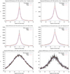 |
Fig. 3 Histograms of angular alignment deviations according to Eq. (5) in Paper I for filamentary structures. Top left: Planck 857 GHz compared with best fit single-channel H I filaments, all sky. Top right: Planck 857 GHz compared with best fit single-channel H I filaments, |b| > 20°. These two plots were replicated from Fig. 3 in Paper I. Center left: Planck 857 GHz compared with best fit filaments from the VDA velocity field pυ, all sky. Center right: Planck 857 GHz compared with best fit filaments from pυ with |b| > 20°. Bottom left: Planck 857 GHz compared with best fit filaments from the VDA density distribution pd, all sky. Bottom right: Planck 857 GHz compared with best fit filaments from the VDA density distribution pd, |b| > 20°. |
5.2 Caustics in p and pv as local diffeomorphisms
Caustics in 2D maps are descending manifolds, associated in case of the observed FIR/H I filamentary structures predominantly with local structures of index one (Sect. 2.1). According to the Morse lemma, these regions can locally be approximated by quadratic functions. These local coordinate transformations describe local diffeomorphisms (Castrigiano & Hayes 2004). Generic critical points are structurally stable, allowing a smooth transition and approximation by quadratic functions. Essential for such an approximation in 2D is that the Hessian matrix has to be nondegenerate. The index of a nondegenerate critical point fully classifies the critical point up to coordinate transformations. The Hessian, Eq. (1), is determined from second derivatives and describes the local curvature. Inspecting Eq. (5), it is easy to see that pυ and pd are derived from p by smooth linear transformations, essentially by subtracting mean intensities and rescaling. The terms 〈pI〉 and 〈p〉〈I〉 in Eq. (5) are constants, applied to the scaling factor  . Linear transformations as in Eq. (5) do not affect the Morse index significantly. Thus, common Morse complexes derived for p and pυ represent local diffeomorphisms, explaining the high correlation coefficients NCC(λ_(p), λ_(pυ)) ≳ 0.98 (see Fig. 1) at high Galactic latitudes.
The concept of local diffeomorphisms simply implies that the transition from p to pυ is defined by a smooth transformation under the condition that the two maps remain differentiable. In other words, two singularities are considered equivalent if and only if there exists a local transformation that maps them into each other. This applies to 97% of the caustics in p that replicate as local diffeomorphisms in pυ.
Understanding Morse complexes, derived from p and pυ databases, as local diffeomorphisms, the assertion that the VDA could derive a completely new set of unexplored velocity caustics data from every spectroscopic data set (Yuen et al. 2021, Sect. 11, item 9) needs to be questioned. The results from Sect. 4, summarized in Table 1 and Fig. 3, indicate that the best alignment between FIR and H I filaments exists for the original unmodified brightness temperatures p. The correlation between filaments in FIR and VDA velocity caustics pυ is weaker, indicating that the VDA algorithm does not quite match the physics of the filamentary ISM.
6 VDA power distributions: Pv and Pd contra P
A fundamental VCA postulate is that turbulent density and velocity fields are statistically uncorrelated for the case of MHD turbulence (Lazarian & Pogosyan 2000, Sect. 6.3.1, Appendix B). For purely isothermal turbulent media global density-velocity correlations are unexpected. Federrath & Banerjee (2015) show however that for non-isothermal multiphase media the Mach number correlates with the gas density (their Fig. 7). Understanding the Mach number as a proxy for turbulent velocities, one expects, depending on the equation of state, that the statistics of velocity and density fluctuations are not independent. The VDA algorithm, Eq. (5), depends by construction on the mathematical definition 〈pυpd〉 = 0 regardless of any actual physics. It is highly misleading to present this relation as an observational fact, as is done by Hu et al. (2023) in their Appendix A.
Assuming independence of density and velocity, VDA aims to separate the contributions arising from density and velocity fluctuations with the corresponding power spectra P = Pυ + Pd. For an evaluation of systematical differences in the power spectra we calculate the averages of Pυ and Pd at high Galactic latitudes. We also relate these contributions to the power P from the raw observations. According to Lazarian & Pogosyan (2000) such power spectra should be steep with power law indices γ < −3. Power law indices derived from channel maps are velocity dependent. To match VCA expectations, we therefore use the steepest power spectra at a velocity of υLSR = 4 km s−1 derived from HI4PI data (see Kalberla & Haud 2019, Fig. 9). For the VDA velocity power spectrum Pυ we obtain a power law index γv = −2.82 ± 0.05, almost identical with γobs = −2.85 ± 0.05 from the observed H I channel map at the same velocity (see Fig. 4). The spectral index γd = −2.87 ± 0.05 for the VDA density is by definition velocity independent and identical to the power law index of the total column density distribution. In summary, Fig. 4 implies that the spectral indices for P, Pυ, and Pd are, within the uncertainties, identical. All power spectra are straight and do not show any bending in contrast to different possible model contributions in Pυ and Pd (see the case studies in Figs. 6 and 7 of Lazarian & Pogosyan 2000). The predicted systematical spectral index changes between Pv, Pd, and P (their Table 1) are not observed.
Velocity decomposition algorithm density fluctuations are marginal and provide only 4% of the observed power. This low level is within the uncertainties consistent with the previous finding (Sect. 4) that Morse complexes of pυ recover 97% of the positions in Morse complexes of p. Figure 4 shows that the power distributions for p and pυ are almost identical. The derived spectral index γ ~ −2.85 is representative of individual probes of the ISM at high Galactic latitudes (see Fig. 9 in the review by McClure-Griffiths et al. 2023). An average index of γ ~ −2.85 ± 0.02 has also been derived by Mittal et al. (2023) after correcting the H I distribution for differences in H I path lengths along the line of sight (see their Fig. 8). Under the VCA constraint that the velocity with the steepest power spectrum should be selected, the decomposition of the observed brightness temperature distribution in VDA velocity caustics pυ and densities pd does not alter the observed spectral index from P. This result is consistent with the investigations in Sect. 4. Statistical similarities in P and Pυ reflect general morphological similarities in p and pυ.
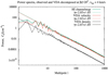 |
Fig. 4 Turbulent power spectra for the observed H I emission p at high Galactic latitudes at a velocity of υLSR = 4 km s−1 compared with power spectra derived from VDA velocity and density contributions pυ and pd. |
7 The physics of FIR/H I Morse complexes
The data that are analyzed in Paper I suggest that filamentary FIR and H I structures, observable at high Galactic latitudes, were shaped by a Galactic small-scale dynamo. This conclusion is based on the filament curvature distribution along the filaments (Paper I, Sect. 4). Furthermore, individual filament-like structures share common morphological properties. Filamentary structures are not individuals; they share a network of filaments. The resulting distribution of aspect ratios 𝒜 and filamentarities is well defined and continuous without clear upper limits in 𝒜 (Paper II). The question arises whether common morphological properties arise from common physical conditions. The FIR filament emission is broadband, but in H I the structures are best reproduced in narrow velocity intervals.
7.1 Spin temperatures and volume densities in H I filaments
In Paper I, it was shown that filaments in H I have low Doppler temperatures. Such temperatures are derived from emission data, and hence the observed line widths are broadened by turbulent motions and the derived Doppler temperatures are only upper limits to the spin temperatures of the H I. With the advent of sensitive absorption surveys it has become feasible to probe FIR/H I filaments for spin temperatures. McClure-Griffiths et al. (2023) collected BIGHICAT, a catalog with 372 unique lines of sight, providing spin temperatures, optical depth, and other properties. We use BIGHICAT to probe spin temperatures within filaments and outside. Figure 3 of McClure-Griffiths et al. (2023) shows the spatial distribution of the absorption components.
BIGHICAT contains 66 positions without detectable absorption; 63 of these positions (95%) are located outside FIR/H I filaments. These 63 positions probe only WNM, which is known to be ubiquitous. The WNM is known to contain no significant small-scale structures, and also has a very low optical depth. From the remaining sources 122 positions need to be disregarded because the associated FIR eigenvalues exceed the threshold λ_ > −1.5 K/deg−2. A total of 37 positions from BIGHICAT close to the Galactic equator are without available spin temperatures, but in 23 of these cases we were able to replace these data by using Gaussian components from the HI4PI survey. This way 174 positions from the absorption survey could be used to determine absorption components at velocities with the closest agreement to observed local filament velocities. These components represent the local physical conditions along the line of sight that are representative for significant FIR/H I filaments. Figure 5 shows the resulting spin temperatures as a function of velocity deviation |∆υLSR|. These velocity deviations represent differences in velocity between the pencil beam pointing to the background source and the closest HI4PI survey position within a filament. Thus, the detectable velocity differences |∆υLSR| represent turbulent velocity fluctuations on scales below 3′.4.
The spin temperatures in Fig. 5 occupy a range 10 ≲ Ts ≲ 500 K, values that are, according to Wolfire et al. (2003), characteristic for the temperature of the CNM. Heiles & Troland (2005) derived a typical CNM temperature of 50 K. The lower display of Fig. 5 shows that these low temperatures are associated with significant FIR eigenvalues in −λ_. There is a trend for lower spin temperatures at positions with lower eigenvalues λ_, but the available data are currently insufficient to establish a significant correlation (r = 0.33). McClure-Griffiths et al. (2023) expect that as soon as the Square Kilometer Array is in full operation, the number of entries in BIGHICAT will increase by several orders of magnitude. Thus, the significance of this correlation can be tested within a few years.
The typical conditions for the CNM in the local multiphase ISM in thermal equilibrium with the WNM can, according to Jenkins & Tripp (2011), be determined from an equilibrium pressure of log(p/k) = 3.58. This results in a typical CNM exitation temperature of 80 K, consistent with Fig. 5. The cooling time for the ISM is in this case estimated by Jenkins & Tripp (2011) to 3 × 10⁴ yr. This timescale is short in comparison to the timescale for the growth of the small-scale magnetic energy, characterized by the viscous eddy turnover time in the order of 105 yr (Schekochihin et al. 2004). The spin temperature depends on excitation processes for the 21 cm line and can for the CNM usually be equated to the exitation temperature (McClure-Griffiths et al. 2023, Sect. 2). Volume densities, derived from absorption observations, are based on the assumption of a local thermal equilibrium. CNM filaments had sufficient time to reach thermal equilibrium, and therefore BIGHICAT data can be used to derive realistic volume densities. The results are shown in Fig. 6; the volume densities are again typical for the CNM, and agree well with the estimates n = 54 cm−3 and n = 80 cm−3 by Heiles & Troland (2005) or Heiles & Haverkorn (2012), respectively. The available sample of absorption features support the interpretation of filaments as cold dense CNM structures. Outside the filaments no absorption and no CNM is detectable.
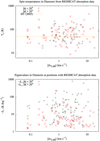 |
Fig. 5 Parameters derived from BIGHICAT data for absorption components with closest match in filament velocities with deviations of |∆υLSR| km s−1 between absorption and emission components. Top: spin temperatures Ts in filaments. The horizontal line indicates the characteristic spin temperature Ts = 50 K, derived by Heiles & Troland (2005). Bottom: eigenvalues −λ_ for the same sample. |
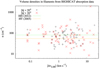 |
Fig. 6 Volume densities n in filaments from BIGHICAT data for absorption components with the closest match in filament velocities with deviations of |∆υLSR| km s−1 between absorption and emission components. The horizontal lines indicate the characteristic volume densities of n = 80 cm−3 derived by Heiles & Haverkorn (2012) and n = 54 cm−3 by Heiles & Troland (2005). |
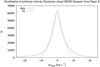 |
Fig. 7 Distribution of turbulent velocity fluctuations ∆υturb along filaments for the sample used in Paper II. The Gaussian fit has a velocity dispersion of σ = 3.8 ± 0.1 km s−1. |
7.2 Turbulent velocity fluctuations
As detailed in Sect. 2.2, H I filaments were matched to FIR filaments using both Hessian eigenvalues and orientation angles (deduced from eigenvectors). In Paper II the resulting set of Morse complexes was decomposed in 6568 individual FIR/H I filaments. For each of these filaments an average radial velocity 〈υfil〉 was determined. Along each of the H I filaments fluctuating radial velocities were observed. We consider these fluctuations as an imprint of the turbulent velocity field ∆υturb(l, b) = (υfil(l, b) − 〈υfil〉) by subtracting for each filament position the average radial velocity 〈υfil〉 from the local filament velocity υfil(l, b). Figure 7 shows the distribution of ∆υturb. The observed turbulent velocity dispersion is σ = 3.8 ± 0.1 km s−1. This is low in comparison to the expected dispersion σ ~ 10 km s−1 in the turbulent ISM (Burkert 2006). The observed ∆υturb distribution is not uniform, however; the median dispersion is ∆υ = 5.24 km s−1. Figure 12 in Paper II shows that filaments with low aspect ratios can have a low velocity dispersion but prominent filaments, with high aspect ratios and covering large surface areas, have enhanced velocity dispersions. These approach the limit σ ~ 10 km s−1. We also note the extended wings in Fig. 7, indicating some local misidentifications in the FIR/H I filaments causing uncertainties in the determination of filament velocities.
Extended cold H I filaments with a typical linewidth of 3 km s−1 (e.g., Paper II, Sect. 3.1) that are exposed to turbulent velocity fluctuations of 3.8–10 km s−1 are affected necessarily by shifts in observed radial velocities. Filaments that are observed in channel maps with a velocity width of 1 km s−1 appear disrupted, and filaments appear to have low aspect ratios. Within PPV channel maps, filament elements that are affected by turbulent velocity fluctuations shift frequently from one velocity channel to another. This leads to an apparent fragmentation and lowers aspect ratios if only channel maps are considered.
Tracing the FIR orientation angle in H I recovers the PPVfil filament geometry in the plane of the sky. Both FIR and H I filaments share common orientation angles. FIR filaments are observed in broadband and the FIR orientation angles are not affected by velocity fluctuations. Tracing FIR orientation angles in H I by fitting (velocity dependent) orientation angles tells us the velocity of the FIR filaments (Clark & Hensley 2019 and Paper II, Sect. 3.3). Thus, the 3D PPV geometry is modified for each individual filament to the 2D case PPVfil, where Vfil stands for the position-dependent filament velocity across the PPV cube. The transformation from PPV to PPVfil represents for each individual filament a smooth transformation (or deformation) of the velocity space. Magnetic fields associated with the filaments suffer from foldings that cause magnetic tension forces with back reactions on the turbulent flow (Schekochihin et al. 2004). In such a scenario, density structures need to be understood as structures in l, b, υLSR, and hence with PPVfil morphology. Each filament occupies an individual PPVfil space. The width of the Vfil slice depends on the observed CNM line width, and is typically 3 km s−1. The Morse complexes that we analyzed need to be understood as manifolds in PPVfil. Since the filaments are disjunct in position, an all-sky PPVfil distribution can be derived.
7.3 VCA velocity mapping in slices
VCA and VDA are theories that are strictly designed for a PPV geometry, decomposing the emission in velocity slices of variable thickness. The claim is that VCA allows a separation of velocity and density fields that affect the PPV data cube, depending on the thickness of the velocity slice. This theory does not allow a local transition of distinct homogeneous filament structures from PPV to PPVfil. The expected role of (hydrodynamic) turbulence is to induce velocity crowding. Filamentary structures are understood as velocity caustics, caused by velocity crowding along the line of sight. Spatially distributed H I along the line of sight is affected by turbulent velocities and mimics density structures in this way. Thus, turbulence moves separate H I components into the same velocity coordinate in PPV space, leading to a merging of these components into a single structure (e.g., Hu et al. 2023, Fig. 1). VCA velocity mapping does not allow us to interpret filamentary structures as real physical objects.
The spectrum of eddies that correspond to most of the turbulent energy at large scales corresponds to the spectrum of thin channel map intensity fluctuations having most of the energy at small scales (Kandel et al. 2016). Lazarian & Yuen (2018) conclude that on scales larger than 3 pc, the intensity of fluctuations in the channel maps is produced to a significant degree by velocity caustics rather than real physical entities (i.e., filaments). This 3 pc scale, derived by Lazarian & Yuen (2018) for a turbulent energy cascade with a steep power spectrum, can be compared with the filament widths of 0.63 pc derived in Paper II for an average filament distance of 250 pc. Velocity mapping is affected by projection effects, but must be spatially coherent in direction perpendicular to the filament. HI4PI data constrain this coherence to 0.63 pc, otherwise the filamentary structures would be smoothed out.
The VCA velocity mapping of distributed H I components along the line of sight to the observed PPV space has consequences for models of the internal structure of FIR filaments. Broadband observations of thermal dust emission are sensitive to the density field, but not to velocity. For FIR/H I filaments the velocity crowding effect implies that several distinct turbulence induced dust components must exist along the line of sight. This is in clear contrast to FIR/H I filaments as coherent structures in PPVfil. Planck Collaboration Int. XLIV. (2016) consider FIR filaments in the diffuse ISM at high Galactic latitudes as density structures; in addition, Planck Collaboration Int. XXXII. (2016) consider them as ridges that are at high Galactic latitudes usually aligned with the magnetic field measured on the structures.
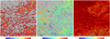 |
Fig. 8 Examples for structures derived with different methods, coordinates are identical with Fig. 2. Left: filaments derived for 857 GHz FIR data in Paper II, shown are eigenvalues −50 < λ_ < −1.5 K/deg−2. Center: PPVfil with color coding in velocity, representing the corresponding velocity field in the range −30 < vLSR < 30 km s−1. Right: caustics in H I column density maps from Paper II, integrated from −50 < vLSR < 50 km s−1 with eigenvalues −250 < λ_ < −5 K/deg−2. |
7.4 FIR filaments and the H I haystack
VCA is based on the analysis of velocity slices with variable thickness, spanning from thin to very broad velocity slices with structures in column density, and claims to reconstruct the underlying velocity and density characteristics. This approach fails, and as a demonstration we want to compare a basic subset of Morse complexes with very thick and thin velocity slices with FIR caustics. Figure 8 first compares FIR filaments with our derived PPVfil results and eigenvalues for HI column densities integrated over the range −50 < vLSR < 50 km s−1. Instead, Fig. 9 covers HI eigenvalues λ_ for channel maps with a 1 km s−1 channel width at velocities −4 < vLSR < 4 km s−1. Fluctuations of the eigenvalue strengths along the filaments are frequent.
7.5 Filament tracing contra velocity slicing
The FIR filaments in the left panel of Fig. 8 are clearly well represented by a rather continuous PPVfil distribution with a well-defined homogeneous velocity structure, including some turbulent velocity fluctuations. This is the result from Paper I, matching FIR and H I structures with both eigenvalues and orientation angles (from eigenvectors). The best fit result was obtained by using local velocity slices with a thickness of 1 km s−1. Increasing the velocity slice thickness leads to a degradation of the results. Comparing FIR filaments (left in Fig. 8) with filaments in column density eigenvalues (right), we find a very complex distribution of filaments in column density. Only a small fraction of the FIR structures can be traced in H I column densities.
Matching FIR filaments with 1 km s−1 broad eigenvalue maps in H I visually is an even more complex task if PPV channel maps are used. Trying to find individual FIR structures within these H I maps in Fig. 9 is like looking for needles in a haystack. The H I distribution is full of filaments. Only a small fraction of these filaments are clearly linked to the FIR. Considering FIR filaments as flux tubes, the filament curvature changes across the tube envelopes (see Sect. 5 of Paper I). Increased curvatures outside the filament centers imply increased curling of magnetic field lines with decreasing field strengths as predicted for the small-scale dynamo.
Comparing the individual maps in Fig. 9 with the FIR and PPVfil in Fig. 8 demonstrates impressively the power of the Hessian operator as a search algorithm for structures if both eigenvalues and eigenvectors (hence orientation angles) are used to match the data. The implication is that H I orientation angles are strongly velocity dependent. Tracing FIR in θ recovers the velocity structure of H I caustics that remain otherwise hidden in velocity slices (channel maps in PPV).
7.6 Velocity gradients for caustics in PPV and PPVfil
Using caustics in PPV in place of PPVfil databases has significant consequences for the determination of velocity gradients. As pointed out by Burkhart (2021), MHD theories predict that velocity fluctuations trace magnetic field fluctuations around turbulent eddies. It is expected that the amplitude of velocity gradients across these eddies should increase with decreasing spatial scale. Thus, velocity gradients are expected as a tracer of magnetic fields on small scales.
The velocity gradient technique (VGT) was first applied by González-Casanova & Lazarian (2017) to PPV data from an isothermal medium. Since then, several publications used VGT with some modifications, we refer to the detailed discussions in Hu et al. (2023). VGT needs to measure gradients in PPV maps from velocity centroids or alternatively from gradient angle maps by averaging over blocks with sizes around 100 × 100 pixels (Lazarian & Yuen 2018). This implies some smoothing. More importantly, VGT does not use caustics to determine velocity gradients.
For the application of the Hessian operator only a 5 × 5 pixel kernel is required. Caustics can be used then in a very simple way to derive velocity gradients on small scales with an average filament width of 0.63 pc at a distance of 250 pc for HI4PI data.
We define
 (10)
(10)
and use she observational available channel width of δvLSR = 1 km s−1. Figure 10 shows PPV gradient maps for she same channels thai are shown in Fig. 9. Comparing the two figures, it is obvious that velocity gradients are small-scale structures, running strictly parallel to the filament ridges.
Applying this gradient technique to She PPVfil database needs the modifiaction
 (11)
(11)
Figure 11 shows the result. The differences between Figs. 10 and 11 are striking, but are readily explained in the context of caustics as descending manifolds. H I filaments represent passes with a narrow width in velocity space. PPVfil filaments are located on top of the passes. The Morse lemma tells us that for smooth functions of variables with a nondegenerate critical point at the origin there exits a local diffeomorphism that preserves the origin and approximates the original function with a quadratic function (e.g., Castrigiano & Hayes 2004). Thus, on top of a saddle it is flat, and gradients are low. Figure 11 shows essentially only noise, but no systematic gradients. As soon as we get to the wings of the descending manifold, gradients may get steep. Backpackers, walking on passes, know this rule by experience. Steep gradients with narrow filamentary structures in Fig. 10 come from the fact that filaments in Fig. 9 are made of CNM, and hence they all have narrow line widths, typically ΔvLSR = 3 km s−1.
The filaments in Fig. 9 and the gradients in Fig. 10 are PPV structures, and hence they represent caustics that are affected by turbulent velocity fluctuations. Orientation angles are known only for a small fraction of these structures associated with FIR filaments. Only for this restricted subset of filamentary structures (Fig. 11) is it possible to separate turbulent contribution and average filament velocities as detailed in Sect. 2.2. These common FIR/H I filaments represent prominent ridges within a network of associated H I filaments.
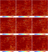 |
Fig. 9 PPV maps of filamentary structures at l = 160°, b = 30° in gnomonic projection. The coordinates are identical to those in Fig. 2. Shown are H I eigenvalues λ_ for p in channel maps with a 1 km s−1 channel width at velocities from −4 km s−1 (top left) to 4 km s−1 (bottom right). |
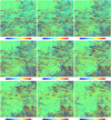 |
Fig. 10 PPV velocity gradient maps according to Eq. (10) for the same velocity channels displayed in Fig. 9. |
8 Summary and conclusion
H I shows for large parts of the diffuse ISM filamentary structures and it is well established that these are correlated with FIR emission and aligned with the ambient magnetic field (e.g., Clark et al. 2014, 2015 or Kalberla et al. 2016). These authors identified the structures with actual H I density filaments. The interpretation of the filaments as density structures is in conflict with Lazarian & Pogosyan (2000). Their VCA postulate is that turbulent velocity fluctuations along the line of sight makes emitting elements at different distances from the observer overlap in velocity space. This effect, also called velocity mapping, causes velocity caustics that are said to be dealt with from a mathematical perspective in Arnold et al. (1985)6. Thus, multiple elements along the line of sight at the same velocity cause enhanced emission in the observations that does not exist in position space (Lazarian & Yuen 2018 and Fig. 1 in Hu et al. 2023).
Following VCA, a number of publications corroborated the velocity caustics model. The discussion about density structures or velocity caustics cumulated with the publications of Lazarian & Yuen (2018) and Clark et al. (2019) in an open conflict. In turn, the existence of dense structures and further the association between FIR structures and H I counterparts was proven (e.g., Clark et al. 2019, Peek & Clark 2019, Clark & Hensley 2019, Murray et al. 2020, Kalberla et al. 2020, Paper I, and Paper II). Filaments were found to be associated with particular cold CNM, an increased CNM fraction and an enhanced FIR emissivity IFIR/NHI.
In response, Yuen et al. (2021) developed a numerical model called VDA to separate velocity and density fluctuations in the VCA framework. This model was supposed to support VCA, and this presentation has been recently reinforced by Hu et al. (2023).
We applied the VDA model to HI4PI observations used by Paper I and Paper II. The main body of our paper is about the performance of the VDA algorithm. Summarizing our results, we note first that structures that were called velocity caustics in the literature are not caustics as defined by Thom (1975) and Arnold et al. (1985) or in the recent literature by Sousbie (2011), among others. VDA velocity and density data are modified data products that, in a way similar to that used for the original observations, may contain caustics. These caustics need to be determined, following the standard procedures explained by Sousbie (2011), Sousbie et al. (2011), Feldbrugge et al. (2018, 2019), among others.
Since the year 2000 has become customary for a group of authors to describe and cite H I structures as velocity caustics without giving any proof that they are actually caustics. In the literature there exists a clear classification of critical points and procedures for deriving caustics, and one would expect such definitions to be followed. Only a small fraction (typically 30%) of the structures visible in VCA/VDA velocity caustic maps pv are related to generic caustics. These filamentary structures, classified as A3 by Arnold et al. (1985), must be worked out before they can be called caustics, otherwise the terminology is misleading. In other words, the caustics of the velocity caustics need to be determined. In the literature, images of velocity caustics are published that do not at all show similarities to the examples of caustics from the observations given here. A few RHT images have been published by Hu et al. (2023), among others, but it is unclear how they are related to FIR structures.
To determine caustics, we applied the same Hessian analysis as in Paper I to the VDA data and found that caustics from VDA velocity data are almost identical with caustics from the original observations. The Pearson product-moment correlation coefficient is ≳98%. Tracing Plank FIR caustics at 857 GHz, we recovered 97% of the filaments from the original H I database with the VDA velocity data. In the mathematical framework of caustics in smooth differentiable maps, caustics from VDA velocity data can be considered as local diffeomorphisms to the caustics from direct H I observations. Thus, the VDA decomposition algorithm does not provide any advantages. Comparing the alignment measures when fitting FIR and H I filament structures, the residual misalignment from fitting uncertainties increases in case of VDA velocity caustics. We conclude that H I filament structures cannot be significantly affected by turbulent velocity crowding, contrary to VCA/VDA predictions. The density model based on original unmodified data performs better. Filaments derived from VDA velocity caustics are correlated in the same way as caustics derived in Paper I, with caustics from broadband FIR emission. The assertion by Hu et al. (2023) that the data analysis in Paper II did not consider velocity caustics is not justified (see Paper I with a preliminary version of Sect. 4).
In the same way as intensity fluctuations in the VDA framework can arise from both density and velocity perturbations, VCA predicts that the observed H I power distribution can be decomposed in velocity and density terms. These can be characterized with narrow and broad velocity channel data and, according to VCA, they should differ significantly from each other. We calculated VDA velocity and density power spectra. The power spectra are straight; there are no significant differences between the VDA velocity power spectrum and the spectrum from the original H I data. All spectral indices agree within the errors. There is no evidence for the VCA predicted change of the power spectrum with respect to the used velocity width, defining velocity, or density effects in VDA.
The VDA predicts significant differences between data products from the original H I data and the decomposed velocity and density terms. The result that VDA velocity data and original H I observations deliver nearly identical caustics rises the question whether the VDA decomposition is based on any physical background. One of the discussed topics is the question whether filamentary H I structures that originate from small-scale fluctuations are linked to the CNM with narrow line widths.
We considered the BIGHICAT compilation of absorption data that are available from McClure-Griffiths et al. (2023). We found that 63 out of 66 observations without detectable absorptions are located outside FIR/H I filaments, and 174 positions from the absorption survey could be used to determine absorption components within FIR/H I filaments. The derived H I spin temperatures and also the corresponding volume densities are typical for temperatures of the CNM. This is not a new result, but for the first time it has been shown that the CNM in the diffuse ISM is exclusively located in filaments with FIR counterparts. We conclude that FIR/H I filaments trace the CNM in the same way as FIR filaments trace cold dust. These caustics are density structures, consistent with previous findings (e.g., Clark et al. 2019, Peek & Clark 2019, Clark & Hensley 2019, Murray et al. 2020, Kalberla et al. 2020, Paper I, and Paper II).
The VCA and descendants, as reviewed by Burkhart (2021), relies on a PPV decomposition algorithm in the channel maps. We demonstrate in Fig. 9 that individual channels in the PPV database are not optimal for the detection and tracing of FIR filaments. In the same way, velocity gradients in PPV are hard to interpret (Fig. 10). In Paper I, it was shown that the distribution of curvatures in filaments follows closely the expected curvature distribution in the case of a turbulence-driven small-scale dynamo. The filament curvature is related to the magnetic field strength (Schekochihin et al. 2004). Sharply curved fields imply a high field tension, and the field strength is reduced. For the small-scale dynamo the magnetic field amplification is exponentially fast and occurs due to stretching of the magnetic field lines by the random velocity shear associated with the turbulent eddies. According to Matthaeus et al. (2008), the local directional alignment of the velocity and magnetic field fluctuations is expected to occur rapidly. However, these calculations missed an important term. The full expression is given by Soler & Hennebelle (2017), their MHD simulations, however, only cover densities n ≳ 3000 cm−3. Densities in our case are far below this value; we observe caustics and velocity gradients that are aligned with the magnetic field. In all cases H I column densities are below NH = 1021.7 cm−3 and the magnetic field is expected to be aligned parallel to the filaments (Hennebelle & Inutsuka 2019).
Observed local H I orientation angles are strongly velocity dependent. This implies that H I filaments must have narrow velocity dispersions. The turbulent velocity field is expected to introduce some local filament bending. In projection, if this happens along the line of side, the bending cannot be observed in position. However, a velocity induced bending causes changes in orientation angle. Filament tracing is therefore a tracing in position on the plane of the sky and is analogous in orientation angle for the velocity along the line of sight. Instead of a PPV alignment we need to consider a PPVfil geometry, tracing the filament also in filament velocity vfil. Such a tracing is provided in a natural way if the Hessian analysis uses the full information, eigenvalues, and eigenvectors (hence orientation angles) from FIR filaments. This PPVfil tracing has to be done for each individual filament and vfil includes position-dependent turbulent velocity fluctuations. In the case that filaments are positionally disjunct (at high Galactic latitudes only a small amount of confusion is expected; see Paper II) the vfil data can be combined to a large-scale velocity field for the filaments.
The significant difference between PPVfil density structures and PPV velocity crowding from the VCA theory is the distribution of matter along the line of sight. In the first case fibers are bent as density structures in PPVfil, in the second case the distribution is fluffy along the line of sight because of different separate components that cause H I velocity crowding. Both approaches can only be consistent if velocity crowding exists on scales that are compatible with the radial extensions of the FIR/H I caustics. Such a solution is however explicitly ruled out by Lazarian & Yuen (2018) for longwave-dominated power spectra with a steep spectral index (γ < −3). A shortwave-dominated or shallow velocity spectrum with γ ≳ −3 is not considered to be physically motivated (Chepurnov & Lazarian 2009).
Our results are in conflict with such theoretical expectations. We get an average multiphase H I spectral index of γ = −2.85. According to McClure-Griffiths et al. (2023), this index is representative for the H I at high Galactic latitudes. For the CNM the power spectrum flattens to γ = −2.5 (Kalberla & Haud 2019), approaching γ = −2.4 as the spectral index of the turbulent magnetic field (Ghosh et al. 2017; Adak et al. 2020). Turbulence in FIR/H I filaments is driven on small scales by a fluctuation dynamo (I), in conflict with a longwave-dominated power law, as assumed by Lazarian & Yuen (2018). Here we argue based on observational results against theoretical expectations7.
Acknowledgements
We acknowledge the referee for careful reading and comments that supported an improvement of the current manuscript. We thank Naomi McClure-Griffiths and Daniel Rybarczyk for help with the BIGHICAT database. We acknowledge the referee of a previous version of this manuscript for constructive comments that helped to improve the quality of this version as a separate paper. HI4PI is based on observations with the 100-m telescope of the MPIfR (Max-Planck- Institut für Radioastronomie) at Effelsberg and the Parkes Radio Telescope, which is part of the Australia Telescope and is funded by the Commonwealth of Australia for operation as a National Facility managed by CSIRO. This research has made use of NASA’s Astrophysics Data System. Some of the results in this paper have been derived using the HEALPix package.
References
- Adak, D., Ghosh, T., Boulanger, F., et al. 2020, A&A, 640, A100 [NASA ADS] [CrossRef] [EDP Sciences] [Google Scholar]
- Arnold, V. I., Varchenko, A., & Gusein-Zade, S. M. 1985, Singularities of Differentiable Maps: Vol. I: The Classification of Critical Points Caustics and Wave Fronts (Boston: Birkhäuser) [Google Scholar]
- Blandford, R. D., & Narayan, R. 1992, ARA&A, 30, 311 [NASA ADS] [CrossRef] [Google Scholar]
- Bond, J. R., Kofman, L., & Pogosyan, D. 1996, Nature, 380, 603 [NASA ADS] [CrossRef] [Google Scholar]
- Burkert, A. 2006, Comptes Rendus Phys., 7, 433 [NASA ADS] [CrossRef] [Google Scholar]
- Burkhart, B. 2021, PASP, 133, 102001 [NASA ADS] [CrossRef] [Google Scholar]
- Castrigiano, D., & Hayes, S. 2004, Catastrophe Theory, 2nd edn. (CRC Press) [Google Scholar]
- Chepurnov, A., & Lazarian, A. 2009, ApJ, 693, 1074 [NASA ADS] [CrossRef] [Google Scholar]
- Clark, S. E., & Hensley, B. S. 2019, ApJ, 887, 136 [NASA ADS] [CrossRef] [Google Scholar]
- Clark, S. E., Peek, J. E. G., & Putman, M. E. 2014, ApJ, 789, 82 [NASA ADS] [CrossRef] [Google Scholar]
- Clark, S. E., Hill, J. C., Peek, J. E. G., et al. 2015, Phys. Rev. Lett., 115, 241302 [NASA ADS] [CrossRef] [Google Scholar]
- Clark, S. E., Peek, J. E. G., & Miville-Deschênes, M.-A. 2019, ApJ, 874, 171 [NASA ADS] [CrossRef] [Google Scholar]
- Esquivel, A., Lazarian, A., Pogosyan, D., et al. 2003, MNRAS, 342, 325 [NASA ADS] [CrossRef] [Google Scholar]
- Federrath, C., & Banerjee, S. 2015, MNRAS, 448, 3297 [NASA ADS] [CrossRef] [Google Scholar]
- Feldbrugge, J., & van de Weygaert, R. 2023, J. Cosmology Astropart. Phys., 2023, 058 [CrossRef] [Google Scholar]
- Feldbrugge, J., van de Weygaert, R., Hidding, J., et al. 2018, J. Cosmology Astropart. Phys., 2018, 027 [CrossRef] [Google Scholar]
- Feldbrugge, J., van Engelen, M., van de Weygaert, R., et al. 2019, J. Cosmology Astropart. Phys., 2019, 052 [CrossRef] [Google Scholar]
- Ghosh, T., Boulanger, F., Martin, P. G., et al. 2017, A&A, 601, A71 [NASA ADS] [CrossRef] [EDP Sciences] [Google Scholar]
- González-Casanova, D. F., & Lazarian, A. 2017, ApJ, 835, 41 [CrossRef] [Google Scholar]
- Heiles, C., & Haverkorn, M. 2012, Space Sci. Rev., 166, 293 [NASA ADS] [CrossRef] [Google Scholar]
- Heiles, C., & Troland, T. H. 2005, ApJ, 624, 773 [NASA ADS] [CrossRef] [Google Scholar]
- Hennebelle, P., & Inutsuka, S.-ichiro 2019, Front. Astron. Space Sci., 6, 5 [NASA ADS] [CrossRef] [Google Scholar]
- HI4PI Collaboration (Ben Bekhti, N., et al.) 2016, A&A, 594, A116 [NASA ADS] [CrossRef] [EDP Sciences] [Google Scholar]
- Ho, K. W., & Lazarian, A. 2023, MNRAS, 520, 3857 [NASA ADS] [CrossRef] [Google Scholar]
- Hu, Y., & Lazarian, A. 2023, MNRAS, 524, 2379 [NASA ADS] [CrossRef] [Google Scholar]
- Hu, Y., Lazarian, A., Alina, D., et al. 2023, MNRAS, 524, 2994 [NASA ADS] [CrossRef] [Google Scholar]
- Jenkins, E. B., & Tripp, T. M. 2011, ApJ, 734, 65 [NASA ADS] [CrossRef] [Google Scholar]
- Jow, D. L., Hill, R., Scott, D., et al. 2018, MNRAS, 474, 1018 [NASA ADS] [CrossRef] [Google Scholar]
- Kalberla, P. M. W., & Haud, U. 2015, A&A, 578, A78 [NASA ADS] [CrossRef] [EDP Sciences] [Google Scholar]
- Kalberla, P. M. W., & Haud, U. 2019, A&A, 627, A112 [NASA ADS] [CrossRef] [EDP Sciences] [Google Scholar]
- Kalberla, P. M. W., & Haud, U. 2020, arXiv e-prints [arXiv:2003.01454] [Google Scholar]
- Kalberla, P. M. W., & Haud, U. 2023, A&A, 673, A101 [NASA ADS] [CrossRef] [EDP Sciences] [Google Scholar]
- Kalberla, P. M. W., Kerp, J., Haud, U., et al. 2016, ApJ, 821, 117 [Google Scholar]
- Kalberla, P. M. W., Kerp, J., & Haud, U. 2020, A&A, 639, A26 [EDP Sciences] [Google Scholar]
- Kalberla, P. M. W., Kerp, J., & Haud, U. 2021, A&A, 654, A91 [NASA ADS] [CrossRef] [EDP Sciences] [Google Scholar]
- Kandel, D., Lazarian, A., & Pogosyan, D. 2016, MNRAS, 461, 1227 [NASA ADS] [CrossRef] [Google Scholar]
- Koch, E. W., & Rosolowsky, E. W. 2015, MNRAS, 452, 3435 [Google Scholar]
- Lazarian, A., & Pogosyan, D. 2000, ApJ, 537, 720 [NASA ADS] [CrossRef] [Google Scholar]
- Lazarian, A., & Pogosyan, D. 2004, ApJ, 616, 943 [NASA ADS] [CrossRef] [Google Scholar]
- Lazarian, A., & Pogosyan, D. 2006, ApJ, 652, 1348 [NASA ADS] [CrossRef] [Google Scholar]
- Lazarian, A., & Pogosyan, D. 2008, ApJ, 686, 350 [NASA ADS] [CrossRef] [Google Scholar]
- Lazarian, A., & Yuen, K. H. 2018, ApJ, 853, 96 [NASA ADS] [CrossRef] [Google Scholar]
- Matthaeus, W. H., Pouquet, A., Mininni, P. D., et al. 2008, Phys. Rev. Lett., 100, 085003 [CrossRef] [Google Scholar]
- McClure-Griffiths, N. M., Stanimirovic, S., & Rybarczyk, D. R. 2023, ARA&A, 61, 19 [NASA ADS] [CrossRef] [Google Scholar]
- Mittal, A. K., Babler, B. L., Stanimirovic, S., et al. 2023, ApJ, 958, 192 [NASA ADS] [CrossRef] [Google Scholar]
- Murray, C. E., Peek, J. E. G., & Kim, C.-G. 2020, ApJ, 899, 15 [CrossRef] [Google Scholar]
- Padoan, P., Juvela, M., Kritsuk, A., et al. 2009, ApJ, 707, L153 [NASA ADS] [CrossRef] [Google Scholar]
- Peek, J. E. G., & Clark, S. E. 2019, ApJ, 886, L13 [NASA ADS] [CrossRef] [Google Scholar]
- Planck Collaboration Int. XXXII. 2016, A&A, 586, A135 [NASA ADS] [CrossRef] [EDP Sciences] [Google Scholar]
- Planck Collaboration Int. XXXV. 2016, A&A, 586, A138 [NASA ADS] [CrossRef] [EDP Sciences] [Google Scholar]
- Planck Collaboration Int. XXXVIII. 2016, A&A, 586, A141 [NASA ADS] [CrossRef] [EDP Sciences] [Google Scholar]
- Planck Collaboration Int. XLIV. 2016, A&A, 596, A105 [NASA ADS] [CrossRef] [EDP Sciences] [Google Scholar]
- Planck Collaboration Int. LVII. 2020, A&A, 643, A42 [NASA ADS] [CrossRef] [EDP Sciences] [Google Scholar]
- Polychroni, D., Schisano, E., Elia, D., et al. 2013, ApJ, 777, L33 [CrossRef] [Google Scholar]
- Schekochihin, A. A., Cowley, S. C., Taylor, S. F., et al. 2004, ApJ, 612, 276 [NASA ADS] [CrossRef] [Google Scholar]
- Schisano, E., Rygl, K. L. J., Molinari, S., et al. 2014, ApJ, 791, 27 [Google Scholar]
- Soler, J. D., & Hennebelle, P. 2017, A&A, 607, A2 [NASA ADS] [CrossRef] [EDP Sciences] [Google Scholar]
- Soler, J. D., Beuther, H., Syed, J., et al. 2020, A&A, 642, A163 [NASA ADS] [CrossRef] [EDP Sciences] [Google Scholar]
- Soler, J. D., Miville-Deschenes, M.-A., Molinari, S., et al. 2022, A&A, 662, A96 [NASA ADS] [CrossRef] [EDP Sciences] [Google Scholar]
- Sousbie, T. 2011, MNRAS, 414, 350 [NASA ADS] [CrossRef] [Google Scholar]
- Sousbie, T., Pichon, C., & Kawahara, H. 2011, MNRAS, 414, 384 [NASA ADS] [CrossRef] [Google Scholar]
- St-Onge, D. A., & Kunz, M. W. 2018, ApJ, 863, L25 [CrossRef] [Google Scholar]
- Thom, R. 1975, Structural Stability and Morphogenesis (New York: Benjamin-Addison-Wesley) [Google Scholar]
- Winkel, B., Kerp, J., Flöer, L., et al. 2016, A&A, 585, A41 [NASA ADS] [CrossRef] [EDP Sciences] [Google Scholar]
- Wolfire, M. G., McKee, C. F., Hollenbach, D., et al. 2003, ApJ, 587, 278 [Google Scholar]
- Xu, S., & Lazarian, A. 2017, New J. Phys., 19, 065005 [NASA ADS] [CrossRef] [Google Scholar]
- Yuen, K. H., & Lazarian, A. 2017, ApJ, 837, L24 [NASA ADS] [CrossRef] [Google Scholar]
- Yuen, K. H., Ho, K. W., & Lazarian, A. 2021, ApJ, 910, 161 [NASA ADS] [CrossRef] [Google Scholar]
The first known drawing of these structures is by Leonardo da Vinci, available as Codex Arundel, folio 86, https://www.bl.uk/catalogues/illuminatedmanuscripts/record.asp?MSID=6454. As a result of a cyber-attack this page at the British Library is currently not available. An alternative link is https://www.leonardodigitale.com/en/browse/codex-arundel/0087-v/
R. Thom received the Fields Medal in 1958 for his contributions to the topology of differentiable manifolds, and was later the founder of catastrophe theory.
A comprehensive introduction to catastrophe theory can be found at https://jfeldbrugge.github.io/Catastrophe-Theory/
FIR filaments with a threshold λ− < −1.5 Kdeg−2, discussed in I, have at high Galactic latitudes for 3% of all positions (6% all sky, respectively) a Morse index of two, and for 26% (39% all sky) an index of one.
Observed data p are brightness temperatures TB as weighted averages over the instrumental velocity window δυ. For consistency with Yuen et al. (2021), we use p in place of TB.
We were unable to find a treatment of mapping effects, such as velocity crowding, in this book.
Hu et al. (2023, Sect. 7.3.6) found that the decomposition of H I observations by Kalberla & Haud (2020) result in steep CNM power spectra in the case of thin channels, suggesting that small-scale CNM structures are rare in thin channels compared to those in thick channels. Our comment on this statement is the following: Single channel CNM power spectra have been shown to be flat, γ ≳ −2.5 (e.g., Kalberla & Haud 2019, Figs. 1, 9, 13, and 23 and Kalberla & Haud 2020, Figs. 3–5). The assertion that small-scale CNM structures are rarer in thin channels than in thick channels is incompatible with H I observations, also with our current results. Observational conflicts with Clark et al. (2019) that might support VCA as reported by Hu et al. (2023) in their Sect. 7.3.6 do not exist.
All Tables
All Figures
|
Fig. 1 Normalized correlation coefficients for eigenvalues in observed intensity p and VDA velocity caustics pυ according to Eq. (5) at high and low Galactic latitudes. Data constrained by λ− < −50 K deg−2 (used in Paper I to compare H I with FIR filaments) and unconstrained eigenvalues are distinguished. |
| In the text | |
|
Fig. 2 Display of example data in gnomonic projection. The field center is at l = 160°, b = 30°, the field size 27°.7. Top left: eigenvalues λ_(pυ) of VDA velocity caustics pυ at υLSR = 0 km s−1. Top right: deviations λ_(pυ) − λ_(p) between eigenvalues from VDA velocity caustics pυ and observed intensities p. Bottom left: velocities υLSR(pυ) of filamentary FIR structures in case of H I filaments derived for VDA velocity caustics pυ. Bottom right: deviations υLSR(pυ) − υLSR(p) from the velocity field υLSR(p) shown in Fig. 6 of Paper I. |
| In the text | |
|
Fig. 3 Histograms of angular alignment deviations according to Eq. (5) in Paper I for filamentary structures. Top left: Planck 857 GHz compared with best fit single-channel H I filaments, all sky. Top right: Planck 857 GHz compared with best fit single-channel H I filaments, |b| > 20°. These two plots were replicated from Fig. 3 in Paper I. Center left: Planck 857 GHz compared with best fit filaments from the VDA velocity field pυ, all sky. Center right: Planck 857 GHz compared with best fit filaments from pυ with |b| > 20°. Bottom left: Planck 857 GHz compared with best fit filaments from the VDA density distribution pd, all sky. Bottom right: Planck 857 GHz compared with best fit filaments from the VDA density distribution pd, |b| > 20°. |
| In the text | |
|
Fig. 4 Turbulent power spectra for the observed H I emission p at high Galactic latitudes at a velocity of υLSR = 4 km s−1 compared with power spectra derived from VDA velocity and density contributions pυ and pd. |
| In the text | |
|
Fig. 5 Parameters derived from BIGHICAT data for absorption components with closest match in filament velocities with deviations of |∆υLSR| km s−1 between absorption and emission components. Top: spin temperatures Ts in filaments. The horizontal line indicates the characteristic spin temperature Ts = 50 K, derived by Heiles & Troland (2005). Bottom: eigenvalues −λ_ for the same sample. |
| In the text | |
|
Fig. 6 Volume densities n in filaments from BIGHICAT data for absorption components with the closest match in filament velocities with deviations of |∆υLSR| km s−1 between absorption and emission components. The horizontal lines indicate the characteristic volume densities of n = 80 cm−3 derived by Heiles & Haverkorn (2012) and n = 54 cm−3 by Heiles & Troland (2005). |
| In the text | |
|
Fig. 7 Distribution of turbulent velocity fluctuations ∆υturb along filaments for the sample used in Paper II. The Gaussian fit has a velocity dispersion of σ = 3.8 ± 0.1 km s−1. |
| In the text | |
|
Fig. 8 Examples for structures derived with different methods, coordinates are identical with Fig. 2. Left: filaments derived for 857 GHz FIR data in Paper II, shown are eigenvalues −50 < λ_ < −1.5 K/deg−2. Center: PPVfil with color coding in velocity, representing the corresponding velocity field in the range −30 < vLSR < 30 km s−1. Right: caustics in H I column density maps from Paper II, integrated from −50 < vLSR < 50 km s−1 with eigenvalues −250 < λ_ < −5 K/deg−2. |
| In the text | |
|
Fig. 9 PPV maps of filamentary structures at l = 160°, b = 30° in gnomonic projection. The coordinates are identical to those in Fig. 2. Shown are H I eigenvalues λ_ for p in channel maps with a 1 km s−1 channel width at velocities from −4 km s−1 (top left) to 4 km s−1 (bottom right). |
| In the text | |
|
Fig. 10 PPV velocity gradient maps according to Eq. (10) for the same velocity channels displayed in Fig. 9. |
| In the text | |
 |
Fig. 11 PPVfil velocity gradient map according to Eq. (11) for comparison with Fig. 10. |
| In the text | |
Current usage metrics show cumulative count of Article Views (full-text article views including HTML views, PDF and ePub downloads, according to the available data) and Abstracts Views on Vision4Press platform.
Data correspond to usage on the plateform after 2015. The current usage metrics is available 48-96 hours after online publication and is updated daily on week days.
Initial download of the metrics may take a while.