| Issue |
A&A
Volume 566, June 2014
|
|
|---|---|---|
| Article Number | A73 | |
| Number of page(s) | 9 | |
| Section | Interstellar and circumstellar matter | |
| DOI | https://doi.org/10.1051/0004-6361/201323065 | |
| Published online | 16 June 2014 | |
Imaging the disk around IRAS 20126+4104 at subarcsecond resolution⋆
1
INAF, Osservatorio Astrofisico di Arcetri, Largo E. Fermi 5,
50125
Firenze,
Italy
e-mail: This email address is being protected from spambots. You need JavaScript enabled to view it.
; This email address is being protected from spambots. You need JavaScript enabled to view it.
; This email address is being protected from spambots. You need JavaScript enabled to view it.
2
Institut de Radioastronomie Millimétrique,
300 rue de la Piscine, 38406 Saint
Martin d’Hères,
France
e-mail:
This email address is being protected from spambots. You need JavaScript enabled to view it.
3
Dublin Institute for Advanced Studies (DIAS),
31 Fitzwilliam Place,
2
Dublin,
Ireland
Received: 15 November 2013
Accepted: 9 May 2014
Abstract
Context. The existence of disks around high-mass stars has yet to be established on a solid ground, as only few reliable candidates are known to date. The disk rotating about the ~104 L⊙ protostar IRAS 20126+4104 is probably the most convincing of these.
Aims. We would like to resolve the disk structure in IRAS 20126+4104 and, if possible, investigate the relationship between the disk and the associated jet emitted along the rotation axis.
Methods. We performed observations at 1.4 mm with the IRAM Plateau de Bure interferometer attaining an angular resolution of ~0.̋4 (~660 AU). We imaged the methyl cyanide J = 12 → 11 ground state and vibrationally excited transitions as well as the CH313CN isotopologue, which had proved to be disk tracers.
Results. Our findings confirm the existence of a disk rotating about a ~7–10 M⊙ star in IRAS 20126+4104, with rotation velocity increasing at small radii. The dramatic improvement in sensitivity and spectral and angular resolution with respect to previous observations allows us to establish that higher excitation transitions are emitted closer to the protostar than the ground state lines, which demonstrates that the gas temperature is increasing towards the centre. We also find that the material is asymmetrically distributed in the disk and speculate on the possible origin of such a distribution. Finally, we demonstrate that the jet emitted along the disk axis is co-rotating with the disk.
Conclusions. We present iron-clad evidence of the existence of a disk undergoing rotation around a B-type protostar, with rotation velocity increasing towards the centre. We also demonstrate that the disk is not axially symmetric. These results prove that B-type stars may form through disk-mediated accretion as their low-mass siblings do, but also show that the disk structure may be significantly perturbed by tidal interactions with (unseen) companions, even in a relatively poor cluster such as that associated with IRAS 20126+4104.
Key words: stars: formation / ISM: jets and outflows / ISM: individual objects: IRAS 20126+4104
Based on observations carried out with the Plateau de Bure interferometer.
© ESO, 2014
1. Introduction
The quest for disks around newly formed early-type stars is one of the challenges of modern astronomy. While there is general consensus that solar-type stars form through disk-mediated accretion, it is still debated whether a scaled-up version of the same formation mechanism holds for high-mass stars. The latter are commonly defined as those stars in excess of ~6–8 M⊙ (Palla & Stahler 1993), a limit that for high accretion rates may become significantly higher (Hosokawa & Omukai 2009). Stars like these reach the zero-age main sequence still undergoing accretion from their parental core. In this situation, the powerful radiation pressure of the star is expected to halt the infalling material, thus preventing further growth of the stellar mass. This so-called radiation pressure problem has recently found a solution that involves accretion through a circumstellar disk. The studies by Krumholtz et al. (2009) and Kuiper et al. (2010; 2011) have demonstrated that stars up to 140 M⊙ can be formed with this mechanism, and basically all current star formation models predict the existence of circumstellar disks around high-mass stars.
The general consensus among theorists on the existence of disks around OB-type stars is in contrast with the lack of observational evidence. To date, only a handful of disk candidates are known, and basically all of these are associated with early B-type stars, whereas disks around the most massive, O-type stars appear elusive (Cesaroni et al. 2007). Very likely, this is due to the difficulty to resolve objects of ≲1000 AU in clustered environments at large distances (typically a few kpc or more). Nonetheless, the important role that circumstellar disks could play in the high-mass star formation process makes such a lack of information very frustrating. While this situation is bound to change with the advent of the Atacama Large Millimeter Array (see results of Sánchez-Monge et al. 2013), it is nonetheless important to consolidate our knowledge of the few convincing examples of disks around B-type stars known to date. We therefore performed new high-angular resolution observations of the best candidate circumstellar disk around a high-mass protostars: IRAS 20126+4104.
This object has been the subject of a long series of studies, which have provided evidence for the presence of a (presumably) Keplerian disk rotating about a ~104 L⊙ protostar and associated with a bipolar jet/outflow undergoing precession about the disk axis (Cesaroni et al. 1997; 1999; 2005; Keto & Zhang 2010; Shepherd et al. 2000; Lebrón et al. 2009; Hofner et al. 1999; 2007; Caratti o Garatti et al. 2008). Multi-epoch VLBI observations of water masers (Moscadelli et al. 2005; 2011) have been used both to study the expansion of the jet and to determine the source distance with great accuracy (1.64 ± 0.05 kpc). More recently, adaptive optics images in the near-IR have permitted us to analyse the structure of the bipolar jet close to the deeply embedded protostar (Cesaroni et al. 2013, hereafter C2013).
Despite the progress made in our knowledge of this object, the structure of the disk and its relationship with the jet remain poorly known, because given the extinction of the dusty envelope around the protostar, only (sub)mm observations at subarcsecond resolution of a suitable molecular line can trace the structure and velocity field of the innermost region inside ~1000 AU from the protostar. The interferometric observations performed by Cesaroni et al. (1997; 1999; 2005) were hindered by limited spectral and/or angular resolution, and could therefore only investigate the disk on a relatively large scale (>1000 AU), where the rotation speed is lower and hence more difficult to measure. With this in mind, we decided to take advantage of the capabilities of the Plateau de Bure interferometer to obtain new images of IRAS 20126+4104 in methyl cyanide, with unprecedented sensitivity and resolution. In this article we report on the results of these observations and shed light on the disk structure and its relationship with the associated bipolar jet on scales ≳100 AU.
2. Observations and data reduction
The data were collected in 2008 on January 29, February 13 and 16, and March 15 with the IRAM six-element array at Plateau de Bure, in the A and B array configurations. We used 2013+370 and 3C 273 as phase and bandpass calibrators, while observations of MWC 349 were used to calibrate the flux density scale. The correlator was tuned at 220.218 GHz in the lower side band, in such a way to cover all the K components of the ground state and vibrationally excited v8 = 1 CH3CN(12–11) transitions, as well as those of the CH313CN isotopomer, but the K = 11 line – although the highest energy lines were not detected. The phase centre of the observations was set at the coordinates α(J2000) =  , δ(J2000) = +41°13′32.̋516).
The data were calibrated, reduced, and analysed with standard procedures, using the GILDAS package1. The typical phase noise was ~30°. Channel maps with natural weighting over the whole frequency range covered were produced resulting in a synthesized half-power beam width (HPBW) of 0.̋46 × 0.̋32 with position angle (PA) of 56°. The line-free channels were identified and used to produce continuum data which were then subtracted from the original data in the u,v domain. Finally, continuum-subtracted cubes were created using natural weigthing. The conversion from flux density per beam to brightness temperature is given by the expression: TB(K) ≃ 169 Sν(Jy / beam).
3. Results
While a large number of lines from different molecules were detected in the broad bandwidth covered by our observations, in the following we will limit our analysis to the transitions of CH3CN and its 13C substituted species CH313CN, as previous studies (Cesaroni et al. 1997; 1999) have proved these to be the best tools to investigate the disk. Also, the CH3CN lines span a large range of excitation energies and opacities, which allows us to sample different layers inside the disk.
3.1. Continuum emission
The continuum map obtained from the line-free channels is shown in Fig. 1. The integrated flux is 0.29 Jy, consistent with the millimetre continuum spectrum derived by Cesaroni et al. (2005, hereafter C2005; see their Fig. 14). From the figure one sees that most of the emission is contained in an almost unresolved structure, whose mean full width at half maximum (FWHM) is ~0.̋5. Applying Gaussian deconvolution, one obtains an intrinsic angular diameter of ~0.̋32 (525 AU) and a brightness temperature corrected for the beam filling factor of ~47 K. Since the maximum measured brightness temperature of the CH3CN lines is ~100 K and the CH3CN rotational temperature is ≲200 K (see Cesaroni et al. 1997), the dust temperature must lie between these two extremes, which implies a dust opacity (along the line of sight through the disk centre) in the range 0.27–0.63. Values like these suggest that the effect of dust absorption could be not entirely negligible even at this relatively long wavelength.
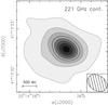 |
Fig. 1 Map of the 1.4 mm continuum emission towards IRAS 20126+ 4104. Contour levels range from 6 to 106.8 mJy/beam in steps of 14.4 mJy/beam (1σ RMS ≃ 1.5 mJy/beam). The white contour corresponds to 50% of the peak flux density. |
An optical depth of 0.27 at 231 GHz, corresponds to an H2 column density (through the disk centre) of ~3 × 1024−3.2 × 1025 cm-2, depending on the dust absorption coefficient adopted (ranging from 0.03 cm2 g-1 of Hildebrand et al. 1983 to 0.0025 cm2 g-1 of the Planck Collaboration XXI 2011). Such a large value is consistent with an edge-on disk and explains why the embedded protostar is not detected even at near-IR wavelengths (Sridharan et al. 2005; C2013). The presence of a prominent temperature and column density peak at the centre is consistent with the gas attaining its maximum temperature and density close to the embedded protostar, as expected.
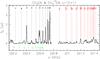 |
Fig. 2 Methyl cyanide spectrum obtained with the Plateau de Bure interferometer towards IRAS 20126+4104. The line emission has been integrated over the core. The dotted lines mark the CH3CN (from top) and CH313CN (from bottom) transitions. The single numbers denote the K component, while the number pairs correspond to the K,l quantum numbers of the vibrationally excited, v8 = 1, transitions. We note how most of the CH3CN and CH313CN components are blended with other methyl cyanide lines and/or with lines of other species. |
It is also worth noting that the compact continuum emission is surrounded by a much fainter halo slightly elongated to the SE, i.e. in the direction of the red-shifted lobe of the jet/outflow (see e.g. C2005). This extension is also seen in the CH3CN lines, and will be discussed in Sect. 4.3.
3.2. Line emission
Figure 2 shows the spectrum obtained by integrating the emission over the region where methyl cyanide was detected (i.e. within ~1′′ from the phase centre). Although this spectrum covers almost all of the ground state and v8 = 1 transitions of CH3CN, as well as those of CH313CN, only few lines are not blended. For this reason, unless otherwise specified, we will analyse only the components that do not overlap significantly with other transitions. These are the K = 2, 3, 4, 8 and v8 = 1 K,l = 1,1 components of CH3CN, and the K = 2 of CH313CN.
In Fig. 3 we show the profiles of the selected transitions, which appear slightly asymmetric and with broad wings. We associate the velocity interval from –10 to +2 km s-1 with the bulk emission, beyond which the line wings become prominent. The maps in Fig. 4 have been obtained by averaging the line emission over this velocity interval. Inspection of the profiles reveals that the asymmetry changes with the energy and opacity of the transition. While the K = 2−4 components appear more prominent in the blue-shifted emission, the K = 8 and K,l = 1,1 lines of CH3CN and the K = 2 CH313CN line are significantly skewed towards the red2. This velocity change may be quantified with the first moment computed in the interval –10 to +2 km s-1, which is –4.2, –4.1, and –3.9 km s-1 for the K = 2,3,4 components, respectively, and –3.3, –3.4 and –2.7 km s-1 for the other three lines. This behaviour is mirrored also in the maps of Fig. 4, where the peak of the emission appears to shift gradually from NE to SW for increasing excitation energy and decreasing opacity, until it coincides with the continuum peak, for the CH3CN K,l = 1,1 and CH313CN K = 2 transitions.
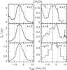 |
Fig. 3 Spectra of the CH3CN and CH313CN transitions that are not significantly affected by blending with other lines. The vertical dashed line denotes the systemic velocity (–3.9 km s-1), while the dotted lines mark the beginning of the line wings. The arrow in the panel of the K = 8 line marks the frequency of the CH2OHCHO(202,18–193,17) transition detected by Beltrán et al. (2009). |
The previous findings suggest that the colder and possibly lower density gas (seen in the CH3CN K = 2, 3, 4 lines) is distributed asymmetrically with respect to the protostar (which should roughly coincide with the mm continuum peak), whereas the hotter gas is found inside a small region around the protostar. This interpretation implies that the disk is not axially symmetric. We will come back to this issue in Sect. 4.1.
Also worth of notice is the slight extension of the emission to the SE, alike to that observed for the continuum emission in Fig. 1. We consider this an indication that a minor fraction of the methyl cyanide emission could come from the red lobe of the bipolar outflow, which extends to the SE of the protostar (see e.g. Cesaroni et al. 1999). Such a result is not surprising, because evidence of CH3CN emission in molecular outflows has been found in other similar objects (see Leurini et al. 2011).
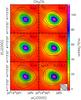 |
Fig. 4 Contour maps of the bulk emission in the same lines as in Fig. 3, obtained by averaging the emission over the velocity interval delimited by the dotted lines in Fig. 3. The background image is the continuum emission shown also in Fig. 1. Contour levels range: from 21.6 to 381.6 in steps of 36 mJy/beam (1σ RMS ≃ 7 mJy/beam) for the K = 2 line; from 22.8 to 402.8 in steps of 38 mJy/beam (1σ RMS ≃ 8 mJy/beam) for the K = 3; from 16.8 to 324.8 in steps of 28 mJy/beam (1σ RMS ≃ 6 mJy/beam) for the K = 4; from 4.5 to 49.5 in steps of 7.5 mJy/beam (1σ RMS ≃ 1.5 mJy/beam) for the K = 2 line of CH313CN; from 8.7 to 95.7 in steps of 14.5 mJy/beam (1σ RMS ≃ 3 mJy/beam) for the K = 8; and from 8.7 to 153.7 in steps of 14.5 mJy/beam (1σ RMS ≃ 3 mJy/beam) for the K,l = 1,1 line. |
4. Analysis and discussion
4.1. Disk structure
An interesting feature revealed by the new CH3CN images is that the disk appears asymmetric with respect to the rotation axis passing through the continuum peak, which we assume to pin point the position of the star. This asymmetry has already been noted in Sect. 3.2 on the basis of the line maps in Fig. 4. Asymmetries are not exceptional in lower mass sources, as demonstrated by the case of the Herbig star Oph IRS 48, where the material turns out to be irregularly distributed in the associated transitional disk (van der Marel et al. 2013; 2014; Bruderer et al. 2014). A method to emphasize our finding and better analyse the physical structure of the disk in IRAS 20126+4104, is to study the distribution of the line emission at different velocities. This can be obtained by fitting all channel maps of a given line with a 2D Gaussian, which provides us with an estimate of the peak position in each velocity channel. Figure 5 compares the distribution of the peaks for the K = 3 component, with those of the K = 8 and K,l = 1,1 lines. Two considerations are in order. The first is that the distribution described by the peaks is significantly more extended to the NE than to the SW. The second is that the higher excitation transitions trace a smaller region than the K = 3 line. The latter finding is consistent with a temperature increase towards the centre of the disk, as expected if the disk is centrally heated. This result is also consistent with previous studies of IRAS 20126+4104, which, assuming a temperature variation with radius of T ∝ Rq, obtain a negative power-law index ranging from q ≲ −1 (Keto & Zhang 2010) to q ≃ −0.57 (C2005). While for a geometrically thin disk one expects q = −0.75 (Pringle 1981), the presence of an envelope in IRAS 20126+4104 and the non-negligible geometrical thickness of the disk (the hydrostatic scale height3 is ≳430 AU) result in a flatter (q > −0.75) temperature profile (see e.g. Chiang & Goldreich 1997). Better angular resolution and modelling are required to derive a precise estimate of the temperature across the disk.
 |
Fig. 5 Distributions of the CH3CN emission peaks at different velocities, obtained with a 2D Gaussian fit to the channel maps of the K = 3 (black points), K = 8 (red), and K,l = 1,1 (green) lines. The cross marks the position of the continuum peak, which we believe to be a good approximation for the location of the protostar. We note how the higher excitation lines trace a region closer to the protostar. |
As for the shorter extent of the disk to the SW, one may wonder whether this might be due to truncation by a nearby companion, perhaps associated with the thermal jet detected by Hofner et al. (1999; 2007) about 0.̋8 to the south of IRAS 20126+4104. A rough estimate of the companion mass Mc needed to cause such a truncation is obtained assuming that the radius of the disk is equal to the radius of the gravitational sphere of influence of the protostar (the Hill radius). From e.g. Eq. (1) of Lissauer & Stevenson (2007), one obtains  (1)where Mc is the mass of the companion, M∗ ≃ 7M⊙ that of the protostar,
  is the length of the radius to the SW of the protostar (see Fig. 5), and dc is the distance of the companion from the protostar. A lower limit to the latter is the projected offset of ~0.̋8 (see above). From Eq. (1) one thus obtains a lower limit Mc > 150 M⊙, too large to be credible.
Perhaps it is more likely that the disk truncation is caused by a nearby, unseen, low-mass companion, located very close to the border of the disk to the SW. Assuming dc ≃ Rd in Eq. (1), one gets Mc ≃ 2 M⊙. As a matter of fact, the presence of a binary system in IRAS 20126+4104 is suggested by the precession of the jet/outflow, as discussed by Shepherd et al. (2000).
Another possibility is that the southern jet is sweeping away the material from the disk, thus causing the observed NE−SW asymmetry, but we cannot exclude that such an asymmetrical distribution of material might be caused by instabilities in the plane of the disk, as suggested by the results illustrated later on in Sect. 4.2.
While these and other hypotheses are purely speculative at the moment, one consideration is in order. Should the disk around IRAS 20126+4104 be affected by any interaction with nearby companions, this would be surprising, because the cluster associated with IRAS 20126+4104 is significantly less populated than the clusters around similar young stellar objects (see Qiu et al. 2008). This result might contain a lesson to learn: if even a poorly populated region can significantly affect the disk structure around a B-type protostar, such an effect should be even more dramatic for disks around O-type (proto)stars, (known to lie inside rich stellar clusters) and could explain why these disks are so elusive (see Sect. 1).
4.2. Disk velocity field
In their study, C2005 have presented evidence that the disk around IRAS 20126+4104 is undergoing Keplerian rotation about a ~7 M⊙ star, up to a radius of at least ~0.03 pc. This conclusion was reached by means of observations of two rotational transitions of C34S, which is sensitive to relatively low densities (~106 cm-3) and traces only the outer, slowly rotating part of the disk. A similar conclusion was reached by Keto & Zhang (2010), who fitted the CH3CN and NH3 line profiles at selected positions across the disk with a numerical model assuming the presence of both a disk and a surrounding envelope undergoing rotation and infall. Their best fit implies a stellar mass of 10.7 M⊙, but values as small as 8.3 M⊙ cannot be ruled out (see their Fig. 9). Our new data allow us to improve on the previous results, because the CH3CN(12−11) lines arise from a denser, hotter, and hence smaller region, where the gravitational field should be dominated by the protostar.
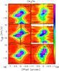 |
Fig. 6 Position–velocity plots along a direction with PA = +37° passing through the continuum peak. The crosses in the bottom left corners denote the spatial and spectral resolutions. Contour levels (in units of brightness temperature in the synthesized beam) range: from 4 to 82 in steps of 13 K (1σ RMS ≃ 1.2 K) for the K = 2 line; from 4 to 74 in steps of 14 K (1σ RMS ≃ 1.2 K) for the K = 3; from 3 to 66 in steps of 9 K (1σ RMS ≃ 0.67 K) for the K = 4; from 2 to 26 in steps of 3 K (1σ RMS ≃ 0.42 K) for the K = 2 line of CH313CN; from 1 to 10 in steps of 3 K (1σ RMS ≃ 0.61 K) for the K = 8; and from 1 to 26 in steps of 5 K (1σ RMS ≃ 0.24 K) for the K,l = 1,1 line. The dashed horizontal and vertical lines correspond to the systemic velocity and position of the 1.4 mm continuum peak. The “butterfly-shaped” patterns in the K = 3 panel outline the regions inside which emission is expected if the gas lies in a disk with radius of 0.̋75 (~1200 AU), rotating about a 7 M⊙ star (solid pattern) and a 10 M⊙ star (dashed). |
To investigate the disk velocity field we have produced position–velocity (PV) plots analogous to those presented by C2005 (see their Fig. 7). These are shown in Fig. 6 and refer to a cut along a direction with PA = +37° passing through the continuum peak. In order to improve the signal to noise of the plots, we also averaged the emission along the direction perpendicular to the cut. We note that this average does not include the CH3CN emission extending to the SE, because this is likely associated with the outflow – as discussed in Sect. 3.2.
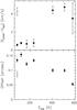 |
Fig. 7 Plots of the peak positions in the PV plots in Fig. 6 versus the energy of the lower level of the corresponding transition. The black points correspond, from left to right, to the K = 2,3,4,5,7,8 and v8 = 1 K,l = 1,1 lines, while the white point denotes the CH313CN K = 2 line. Top: absolute value of the relative velocity of the peak with respect to the systemic velocity, Vsys ≃ −3.9 km s-1. The bars correspond to half the velocity channel. Bottom: absolute value of the distance of the peak from the position of the continuum peak, measured along the plane of the disk (i.e. along the direction with PA = +37°). |
For the sake of comparison, we overlay on the PV plot of the K = 3 line, the patterns encompassing the regions from which emission is expected in the cases of a Keplerian disk rotating about a 7 M⊙ (C2005) and 10 M⊙ (Keto & Zhang 2010) star. Clearly, these are not intended to fit the data (as they do not consider the line width and the limited angular resolution), but have the sole purpose to outline the “butterfly-shaped” pattern of the emission, typical of rotation curves with velocity (Vrot) increasing towards the centre. A special case is that of Keplerian rotation, where Vrot ∝ R−1/2. Here, a caveat is in order. Both C2005 and Keto & Zhang (2010) obtained a satisfactory fit to the data, assuming a priori a velocity field for the disk (+envelope), but neither study demonstrates that Keplerian rotation is the best possible rotation curve. Thus, other laws of the type Vrot ∝ Rα with α < 0 and α ≠ −1/2 might give a better fit, as in the case of the Herbig Ae star AB Aur where significant deviations from Keplerian rotation have been found (Pietu et al. 2005; Tang et al. 2012). With this in mind, in the following we will refer to the velocity field of the disk in IRAS 20126+4104 as (quasi-)Keplerian rotation.
In the PV plots, the asymmetry of the emission in the plane of the disk shows up more remarkably than in Figs. 3 and 4. Clearly, the transitions with the highest opacities and lowest excitations present a peak of emission to the NE, at low velocities (~1 km s-1 relative to the systemic velocity), whereas at higher energies and lower optical depths the emission peak moves to the SW at significantly higher speeds (≳4 km s-1). Figure 7 illustrates this effect, by reporting the velocity (Vpeak) and position of the peak in each PV plot versus the excitation energy of the corresponding transition. The positions have been obtained with a 2D Gaussian fit to the emission in the channel corresponding to Vpeak and the error has been computed from Eq. (1) of Reid et al. (1988). The velocity in Fig. 7 is computed relative to the systemic velocity (in absolute value) i.e. relative to the protostar, while the offset is the projected distance (in absolute value) from the continuum peak, which best approximates the stellar position. We note that to sample as many energy levels as possible, we have used also the K = 5 and 7 components, as these are only partially overlapped to CH313CN lines. The K = 6 component is unusable because heavily blended with the HNCO(101 9−91 8) line.
Velocity components along the line of sight and positions in the plane of the disk, of the peaks in the PV plots of various CH3CN and CH313CN lines.
Our findings support the reasonable expectation that the lower energy lines are emitted farther away from the star than the higher-excitation and/or lower-opacity transitions, because the latter are seen at larger offsets and lower velocities than the former. One can obtain a more quantitative estimate of the locations where the different lines are emitted. For the sake of simplicity, in the following we assume that the disk is undergoing pure Keplerian rotation. While the results may be quantitatively different for quasi-Keplerian rotation, the qualitative conclusions obtained below will not change significantly. In a Keplerian disk, the component of the rotational velocity along the line of sight is given by the expression  (2)where V is normalized with respect to the rotational speed at a given radius, x is the impact parameter normalized with respect to that radius, and y is the coordinate along the line of sight, also normalized with respect to the same radius. From this, one can trivially obtain the value of y as
  (3)where we assume that the negative solution corresponds to the part of the disk facing the observer.
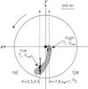 |
Fig. 8 CH3CN disk around IRAS 20126+4104. The observer lies at y = −∞ and sees the disk edge on. The curved arrow indicates the sense of rotation. The points mark the estimated positions of the same peaks as in Fig. 7, and colour-coded in the same way. The grey area outlines a tentative trailing spiral arm. The starred symbol marks the position of the protostar and the two dashed lines are two lines of sight crossing the regions where the low- and high-energy lines peak. The two solid arrows indicate the two regions where the observed lines are emitted. |
Using the values of the impact parameters and velocities in Fig. 7 and assuming a disk radius of 0.̋75 and a corresponding velocity of 2.25 km s-1 (i.e. a central star of ~7 M⊙ – see the Keplerian pattern in Fig. 6), one can compute the values of y and hence locate the positions in the plane of the disk, where the various lines are emitted. These are listed in Table 1 and drawn in Fig. 8, where a sketch of the disk seen face on is presented. We have arbitrarily adopted the negative solution in Eq. (3). For the low-K lines this choice is justified because the emission from the farthest point (y > 0) along the line of sight (l.o.s.) is likely to be self-absorbed at the closest point (at y < 0), due to the large line opacity4. For the CH313CN and higher-excitation lines our assumption is more questionable, as they are likely optically thin. However, the corresponding points lie very close to the plane of the sky (i.e. at y ≃ 0; see Fig. 8), so the choice of the sign is quite unimportant.
The distribution of the points in Fig. 8 confirms that the lower energy lines are mostly arising in the outer region of the disk to the NE, whereas the higher excitation/lower optical depth transitions come from the inner region seen to the SW.
These results provide clear evidence of an asymmetric distribution of material in the disk. The question is whether such an asymmetry is due to inhomogeneities randomly distributed across the disk or instead mirrors a specific phenomenon strictly related to the accretion process and/or the dynamics of the disk itself. Clearly, the data available to us do not permit us to answer this question, but we can provide the reader with some speculations.
One possibility is that we are observing a spiral arm, as tentatively depicted in Fig. 8. The existence of spiral density structures is indeed predicted by numerical calculations and appears to become more prominent for increasing stellar masses (see e.g. Cossins et al. 2009, Kratter et al. 2010). We therefore believe that this possibility in the case of IRAS 20126+4104 cannot be disregarded. Alternatively, density enhancements might be provoked by material accreting onto the disk and, eventually, the protostar, alike to the infalling filaments observed by Tobin et al. (2012) in a number of low-mass young stellar objects. It is reasonable to expect that the interactions between the infalling envelope and the circumstellar disk are more prominent in the deeply embedded high-mass protostars than in their low-mass siblings. Finally, one cannot exclude that the disk structure may be affected by nearby companions, as already discussed in Sect. 4.1. These could generate instabilities and even open gaps in the disk, thus breaking the axial symmetry.
It is worth noting that, to some extent, our case resembles that of the lower-mass, Herbig Ae star AB Aur, where evidence for the existence of residual accretion, disk asymmetries, and spiral arms has been found (see Tang et al. 2012). However, the linear resolution attained in our case is an order of magnitude worse than that of the AB Aur observations, so that any comparison between the two objects is to be considered with caution. Higher resolution (≲0.̋1) images are needed to draw any firm conclusion and discriminate between the different hypotheses to explain the observed asymmetrical distribution of the gas in the plane of the disk of IRAS 20126+4104.
4.3. The disk–jet connection
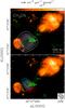 |
Fig. 9 Overlay of the bulk (top panel) and blue- and red-shifted emission (bottom panel) of the CH3CN K = 3 line on the image of the H2 2.2 μm line emission obtained by C2013. The green points and arrows denote the H2O maser spots and associated proper motions measured by Moscadelli et al. (2005). Contour levels in the top panel are the same as in Fig. 4, while in the bottom panel range from 15 to 225 in steps of 30 mJy/beam. |
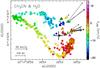 |
Fig. 10 Map of the peaks of the CH3CN K = 2,3,4 line emission (circles) and water maser spots (triangles) from Moscadelli et al. (2000; 2005) and Edris et al. (2005). The colour indicates the LSR velocity according to the code reported in the scale to the right. The arrows indicate the proper motions measured by Moscadelli et al. (2005). The cross marks the position of the continuum emission peak. |
Since one of the goals of the present study is to investigate the relationship between the disk and the associated jet/outflow, we compare the CH3CN emission to the near-IR images of C2013, which provide us with excellent information on the jet structure close to the protostar. This is done in Fig. 9, where both the bulk (top panel) and the blue- and red-shifted CH3CN K = 3 emission are overlaid on an image of the 2.2 μm H2 line emission. In the same figure, we also plot the proper motions of the water masers measured by Moscadelli et al. (2005).
Cesaroni et al. (2013) propose that the ejection episodes from the protostar occur at different times in the SE and NW lobes. In fact, the mushroom-shaped H2 structure to the NW lies at a larger distance from the protostar than the bubble of H2 emission seen to the SE. The interpretation of C2013 is that the latter corresponds to a more recent ejection episode than the former. The H2O maser spots expanding to the NW are likely associated with an even younger ejection, still piercing the surrounding envelope. This explains why no IR emission is seen close to the masers. Our data appear to confirm the scenario depicted by C2013, because the CH3CN contours are slightly extended towards the SE bubble, as if the emission were tracing the walls of the cavity encompassing the SE jet lobe. This opens up farther away from the star allowing the near-IR photons to escape and form the observed bubble. On the opposite side, the CH3CN emission drops sharply, right where the H2O masers appear. This suggests that CH3CN is not excited beyond a few 100 AU to the NW of the protostar, possibly because of the dense, cold material against which the NW lobe is colliding.
It is believed that the expansion of the jets from low-mass (proto)stars could be driven by a mechanism involving a magnetic field corotating with the circumstellar disk. Indeed, in some cases evidence of jet rotation about its axis has been found (see e.g. Coffey et al. 2007). It is therefore of interest to find out whether this might be the case also for high-mass (proto)stars. Moreover, the existence of jet rotation would be strong evidence in favour of the existence of a disk rotating about the jet axis.
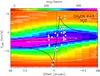 |
Fig. 11 Same as Fig. 6 for the CH3CN K = 3 line, with overlaid points (triangles) representing the H2O maser spots shown in Fig. 10. |
With this in mind, we have compared the velocity field of the disk around IRAS 20126+4104 with that of the associated jet, within a few 100 AU from the surface of the disk itself. For this purpose, we have used the results of the 2D Gaussian fit described above. This is illustrated in Fig. 10, where the peaks of the K = 2,3,4 components are shown as circles, with colour corresponding to the velocity associated with each peak. As expected for (quasi-)Keplerian rotation, the highest velocities are attained close to the disk centre, i.e. close to the protostar, whose position reasonably corresponds to the continuum peak. The only tracer that can be used to study the velocity field of the jet on the same scale are the H2O masers imaged with the VLBI by Moscadelli et al. (2000; 2005) and with MERLIN by Edris et al. (2005). These are plotted as triangles in the same figure5.
The maser 3D velocities are dominated by an expansion component along the jet of the order of ~50−100 km s-1, which affects also the observed velocity along the l.o.s.. Therefore, if we want to unveil a possible rotational component of the jet, the expansion component must be subtracted from the maser l.o.s. velocities. If one calculates the mean velocity along the l.o.s. of all the H2O maser spots (Vmean ≃ −9.4 km s-1), the resulting azimuthal component should be zero because for each spot rotating towards the observer, ideally there should be another spot rotating away from it. In contrast, the expansion velocities are all very similar because the jet is very collimated, and hence their mean value is a good approximation to the effective LSR velocity of each spot due only to the expansion. The effective expansion speed along the l.o.s. is then obtained as Vexp = Vmean − Vsys ≃ −5.5 km s-1, where Vsys ≃ −3.9 km s-1 is the systemic velocity of IRAS 20126+4104. Finally, Vexp was subtracted from the LSR velocities of the maser spots.
The result is shown in Fig. 10, where the same colour coding has been used for both the LSR velocities of the CH3CN peaks and those of the H2O maser spots. Interestingly, one sees that most of the spots to the SW are red-shifted, while most of those to the NE are blue-shifted, consistent with the disk rotation velocity traced by methyl cyanide. This result is seen also in the PV plot in Fig. 11, where the points representing the H2O maser spots are overlaid on the PV plot of the CH3CN K = 3 component and compared to the pattern of a Keplerian disk rotating about a 7 M⊙ star. One sees that 22 out of 26 (85%) of the SW spots are red shifted, and 17 out of 25 (68%) of the NE spots are blue shifted, and their velocities are consistent with those of the CH3CN emission. This is strong evidence that the jet is tightly connected to the disk, at least on scales as small as a few 100 AU.
In conclusion, we stress that our findings not only indicate that the jet in IRAS 20126+4104 is rotating about its axis, but also confirm that the velocity gradient observed in CH3CN is due to rotation about the same axis. This result strongly indicates that the methyl cyanide emission is tracing a circumstellar rotating disk around IRAS 20126+4104.
5. Summary and conclusions
We performed interferometric observations of methyl cyanide rotational transitions towards the high-mass protostar IRAS 20126+4104, for which convincing evidence for the existence of a circumstellar disk had been found. Our results confirm that the CH3CN emission is indeed tracing a (quasi-)Keplerian disk rotating about a 7−10 M⊙ protostar and demonstrate that the material is asymmetrically distributed in the plane of the disk.
We show that gravitational interactions with a nearby low-mass companion could significantly affect the disk structure and hence determine the observed disk asymmetry. Since the stellar cluster associated with IRAS 20126+4104 is known to be less populated than average (Qiu et al. 2008), our findings suggest that tidal interactions might be very effective in perturbing disks around massive stars and thus explain why disks around O-stars, surrounded by rich clusters, have been until now so elusive.
Finally, comparison between previous H2O maser data tracing the jet from IRAS 20126+4104 and our new CH3CN data reveal that the jet is rotating about its axis. This finding not only constrains the genesis of the jet, but also provides us with further, iron-clad evidence that the velocity gradient observed in CH3CN is indeed tracing rotation about the jet axis.
The GILDAS software has been developed at IRAM and Observatoire de Grenoble – see http://www.iram.fr/IRAMFR/GILDAS
The scale height, H, has been computed from the expression H = (FWHM/ obtained by replacing cs with FWHM/
 in Eq. (3.14) of Pringle (1981) and assuming FWHM ≃ 3 km s-1, Mstar ≲ 10M⊙, and Rdisk ≃ 1000 AU.
The mean optical depth over the CH3CN(12–11) K = 2 line, estimated from the ratio to the same CH313CN transition, is ~7, assuming an isotopic abundance ratio [12C/13C] = 76 (Wilson & Rood 1994).
Unlike C2013, we made no attempt to improve on the relative astrometrical accuracy between the CH3CN and H2O positions. However, we caution the reader that the relative positional error may be as large as a significant fraction of the PdBI beam (≲0.̋3).
Acknowledgments
The authors gratefully acknowledge the IRAM technical staff for their support in this project. It is also a pleasure to thank Francesca Bacciotti for stimulating discussions about the physics of jets from YSOs.
References
- Beltrán, M. T., Codella, C., Viti, S., Neri, R., & Cesaroni, R. 2011, A&A, 525, A151 [NASA ADS] [CrossRef] [EDP Sciences] [Google Scholar]
- Bruderer, S., van der Marel, N., van Dishoeck, E. F., & van Kempen, T. A. 2014, A&A, 562, A26 [NASA ADS] [CrossRef] [EDP Sciences] [Google Scholar]
- Caratti o Garatti, A., Froebrich, D., Eislöffel, J., Giannini, T., & Nisini, B. 2008, A&A, 485, 137 [NASA ADS] [CrossRef] [EDP Sciences] [Google Scholar]
- Cesaroni, R., Felli, M., Testi, L., Walmsley, C. M., & Olmi, L. 1997, A&A, 325, 725 [NASA ADS] [Google Scholar]
- Cesaroni, R., Felli, M., Jenness, T., et al. 1999, A&A, 345, 949 [NASA ADS] [Google Scholar]
- Cesaroni, R., Neri, R., Olmi, L., et al. 2005, A&A, 434, 1039 (C2005) [NASA ADS] [CrossRef] [EDP Sciences] [Google Scholar]
- Cesaroni, R., Galli, D., Lodato, G., Walmsley, C. M., & Zhang, Q. 2007, in Protostars and Planets V, eds. B. Reipurth, D. Jewitt, & K. Keil (Tucson: Univ. of Arizona Press), 197 [Google Scholar]
- Cesaroni, R., Massi, F., Arcidiacono, C., et al. 2013, A&A, 549, A146 (C2013) [NASA ADS] [CrossRef] [EDP Sciences] [Google Scholar]
- Chiang, E. I., & Goldreich, P. 1997, ApJ, 490, 368 [NASA ADS] [CrossRef] [Google Scholar]
- Cossins, P., Lodato, G., & Clarke, C. J. 2009, MNRAS, 393, 1157 [Google Scholar]
- Coffey, D., Bacciotti, F., Ray, T. P., Eislöffel, J., & Woitas, J. 2007, ApJ, 663, 350 [NASA ADS] [CrossRef] [Google Scholar]
- Edris, K. A., Fuller, G. A., Cohen, R. J., & Etoka, S. 2005, A&A, 434, 213 [NASA ADS] [CrossRef] [EDP Sciences] [Google Scholar]
- Hildebrand, R. H. 1983, QJRAS, 24, 267 [NASA ADS] [Google Scholar]
- Hofner, P., Cesaroni, R., Rodríguez, L. F., & Martí, J. 1999, A&A, 345, L43 [NASA ADS] [Google Scholar]
- Hofner, P., Cesaroni, R., Olmi, L., et al. 2007, A&A, 465, 197 [NASA ADS] [CrossRef] [EDP Sciences] [Google Scholar]
- Hosokawa, T., & Omukai, K. 2009, ApJ, 691, 823 [NASA ADS] [CrossRef] [Google Scholar]
- Keto, E. H., & Zhang, Q. 2010, MNRAS, 406, 102 [NASA ADS] [CrossRef] [Google Scholar]
- Kratter, K. M., Matzner, C. D., Krumholz, M. R., & Klein, R. I. 2010, ApJ, 708, 1585 [NASA ADS] [CrossRef] [Google Scholar]
- Krumholz, M. R., Klein, R. I., McKee, C. F., Offner, S. S. R., & Cunningham, A. J. 2009, Science, 323, 754 [NASA ADS] [CrossRef] [PubMed] [Google Scholar]
- Kuiper, R., Klahr, H., Beuther, H., & Henning, Th. 2010, ApJ, 722, 1556 [CrossRef] [Google Scholar]
- Kuiper, R., Klahr, H., Beuther, H., & Henning, Th. 2011, ApJ, 732, 20 [NASA ADS] [CrossRef] [Google Scholar]
- Lebrón, M., Beuther, H., Schilke, P., & Stanke, Th. 2006, A&A, 448, 1037 [NASA ADS] [CrossRef] [EDP Sciences] [Google Scholar]
- Leurini, S., Codella, C., Zapata, L., et al. 2011, A&A, 530, A12 [NASA ADS] [CrossRef] [EDP Sciences] [Google Scholar]
- Lissauer, J. J., & Stevenson, D. J. 2007, in Protostars and Planets V, eds. B. Reipurth, D. Jewitt, & K. Keil (Tucson: Univ. of Arizona Press), 591 [Google Scholar]
- Moscadelli, L., Cesaroni, R., & Rioja, M. J. 2000, A&A, 360, 663 [NASA ADS] [Google Scholar]
- Moscadelli, L., Cesaroni, R., & Rioja, M. J. 2005, A&A, 438, 889 [NASA ADS] [CrossRef] [EDP Sciences] [Google Scholar]
- Moscadelli, L., Cesaroni, R., Rioja, M. J., Dodson, R., & Reid, M. J. 2011, A&A, 526, A66 [NASA ADS] [CrossRef] [EDP Sciences] [Google Scholar]
- Palla, F., & Stahler, S. W. 1993, ApJ, 418, 414 [NASA ADS] [CrossRef] [Google Scholar]
- Piétu, V., Guilloteau, S., & Dutrey, A. 2005, A&A, 443, 945 [NASA ADS] [CrossRef] [EDP Sciences] [Google Scholar]
- Planck Collaboration XXI 2011, A&A, 536, A21 [NASA ADS] [CrossRef] [EDP Sciences] [Google Scholar]
- Pringle, J. E. 1981, ARA&A, 19, 137 [NASA ADS] [CrossRef] [Google Scholar]
- Qiu, K., Zhang, Q., Megeath, S. T., et al. 2008, ApJ, 685, 1005 [NASA ADS] [CrossRef] [Google Scholar]
- Reid, M. J., Schneps, M. H., Moran, J. M., et al. 1988, ApJ, 330, 809 [NASA ADS] [CrossRef] [Google Scholar]
- Sánchez-Monge, Á., Cesaroni, R., Beltrán, M. T., et al. 2013, A&A, 552, L10 [NASA ADS] [CrossRef] [EDP Sciences] [Google Scholar]
- Shepherd, D. S., Yu, K. C., Bally, J., & Testi, L. 2000, ApJ, 535, 833 [Google Scholar]
- Sridharan, T. K., Williams, S. J., & Fuller, G. A. 2005, ApJ, 631, L73 [NASA ADS] [CrossRef] [Google Scholar]
- Tang, Y.-W., Guilloteau, S., Piétu, V., et al. 2012, A&A, 547, A84 [NASA ADS] [CrossRef] [EDP Sciences] [Google Scholar]
- Tobin, J. J., Hartmann, L., Bergin, E., et al. 2012, ApJ, 748, 16 [Google Scholar]
- van der Marel, N., van Dishoeck, E. F., Bruderer, S., et al. 2013, Science, 340, 1199 [NASA ADS] [CrossRef] [PubMed] [Google Scholar]
- van der Marel, N., van Dishoeck, E. F., Bruderer, S., & van Kempen, T. A. 2014, A&A, 563, A113 [NASA ADS] [CrossRef] [EDP Sciences] [Google Scholar]
- Wilson, T. L., & Rood, R. 1994, ARA&A, 32, 191 [NASA ADS] [CrossRef] [Google Scholar]
All Tables
Velocity components along the line of sight and positions in the plane of the disk, of the peaks in the PV plots of various CH3CN and CH313CN lines.
All Figures
|
Fig. 1 Map of the 1.4 mm continuum emission towards IRAS 20126+ 4104. Contour levels range from 6 to 106.8 mJy/beam in steps of 14.4 mJy/beam (1σ RMS ≃ 1.5 mJy/beam). The white contour corresponds to 50% of the peak flux density. |
| In the text | |
|
Fig. 2 Methyl cyanide spectrum obtained with the Plateau de Bure interferometer towards IRAS 20126+4104. The line emission has been integrated over the core. The dotted lines mark the CH3CN (from top) and CH313CN (from bottom) transitions. The single numbers denote the K component, while the number pairs correspond to the K,l quantum numbers of the vibrationally excited, v8 = 1, transitions. We note how most of the CH3CN and CH313CN components are blended with other methyl cyanide lines and/or with lines of other species. |
| In the text | |
|
Fig. 3 Spectra of the CH3CN and CH313CN transitions that are not significantly affected by blending with other lines. The vertical dashed line denotes the systemic velocity (–3.9 km s-1), while the dotted lines mark the beginning of the line wings. The arrow in the panel of the K = 8 line marks the frequency of the CH2OHCHO(202,18–193,17) transition detected by Beltrán et al. (2009). |
| In the text | |
|
Fig. 4 Contour maps of the bulk emission in the same lines as in Fig. 3, obtained by averaging the emission over the velocity interval delimited by the dotted lines in Fig. 3. The background image is the continuum emission shown also in Fig. 1. Contour levels range: from 21.6 to 381.6 in steps of 36 mJy/beam (1σ RMS ≃ 7 mJy/beam) for the K = 2 line; from 22.8 to 402.8 in steps of 38 mJy/beam (1σ RMS ≃ 8 mJy/beam) for the K = 3; from 16.8 to 324.8 in steps of 28 mJy/beam (1σ RMS ≃ 6 mJy/beam) for the K = 4; from 4.5 to 49.5 in steps of 7.5 mJy/beam (1σ RMS ≃ 1.5 mJy/beam) for the K = 2 line of CH313CN; from 8.7 to 95.7 in steps of 14.5 mJy/beam (1σ RMS ≃ 3 mJy/beam) for the K = 8; and from 8.7 to 153.7 in steps of 14.5 mJy/beam (1σ RMS ≃ 3 mJy/beam) for the K,l = 1,1 line. |
| In the text | |
|
Fig. 5 Distributions of the CH3CN emission peaks at different velocities, obtained with a 2D Gaussian fit to the channel maps of the K = 3 (black points), K = 8 (red), and K,l = 1,1 (green) lines. The cross marks the position of the continuum peak, which we believe to be a good approximation for the location of the protostar. We note how the higher excitation lines trace a region closer to the protostar. |
| In the text | |
|
Fig. 6 Position–velocity plots along a direction with PA = +37° passing through the continuum peak. The crosses in the bottom left corners denote the spatial and spectral resolutions. Contour levels (in units of brightness temperature in the synthesized beam) range: from 4 to 82 in steps of 13 K (1σ RMS ≃ 1.2 K) for the K = 2 line; from 4 to 74 in steps of 14 K (1σ RMS ≃ 1.2 K) for the K = 3; from 3 to 66 in steps of 9 K (1σ RMS ≃ 0.67 K) for the K = 4; from 2 to 26 in steps of 3 K (1σ RMS ≃ 0.42 K) for the K = 2 line of CH313CN; from 1 to 10 in steps of 3 K (1σ RMS ≃ 0.61 K) for the K = 8; and from 1 to 26 in steps of 5 K (1σ RMS ≃ 0.24 K) for the K,l = 1,1 line. The dashed horizontal and vertical lines correspond to the systemic velocity and position of the 1.4 mm continuum peak. The “butterfly-shaped” patterns in the K = 3 panel outline the regions inside which emission is expected if the gas lies in a disk with radius of 0.̋75 (~1200 AU), rotating about a 7 M⊙ star (solid pattern) and a 10 M⊙ star (dashed). |
| In the text | |
|
Fig. 7 Plots of the peak positions in the PV plots in Fig. 6 versus the energy of the lower level of the corresponding transition. The black points correspond, from left to right, to the K = 2,3,4,5,7,8 and v8 = 1 K,l = 1,1 lines, while the white point denotes the CH313CN K = 2 line. Top: absolute value of the relative velocity of the peak with respect to the systemic velocity, Vsys ≃ −3.9 km s-1. The bars correspond to half the velocity channel. Bottom: absolute value of the distance of the peak from the position of the continuum peak, measured along the plane of the disk (i.e. along the direction with PA = +37°). |
| In the text | |
|
Fig. 8 CH3CN disk around IRAS 20126+4104. The observer lies at y = −∞ and sees the disk edge on. The curved arrow indicates the sense of rotation. The points mark the estimated positions of the same peaks as in Fig. 7, and colour-coded in the same way. The grey area outlines a tentative trailing spiral arm. The starred symbol marks the position of the protostar and the two dashed lines are two lines of sight crossing the regions where the low- and high-energy lines peak. The two solid arrows indicate the two regions where the observed lines are emitted. |
| In the text | |
|
Fig. 9 Overlay of the bulk (top panel) and blue- and red-shifted emission (bottom panel) of the CH3CN K = 3 line on the image of the H2 2.2 μm line emission obtained by C2013. The green points and arrows denote the H2O maser spots and associated proper motions measured by Moscadelli et al. (2005). Contour levels in the top panel are the same as in Fig. 4, while in the bottom panel range from 15 to 225 in steps of 30 mJy/beam. |
| In the text | |
|
Fig. 10 Map of the peaks of the CH3CN K = 2,3,4 line emission (circles) and water maser spots (triangles) from Moscadelli et al. (2000; 2005) and Edris et al. (2005). The colour indicates the LSR velocity according to the code reported in the scale to the right. The arrows indicate the proper motions measured by Moscadelli et al. (2005). The cross marks the position of the continuum emission peak. |
| In the text | |
|
Fig. 11 Same as Fig. 6 for the CH3CN K = 3 line, with overlaid points (triangles) representing the H2O maser spots shown in Fig. 10. |
| In the text | |
Current usage metrics show cumulative count of Article Views (full-text article views including HTML views, PDF and ePub downloads, according to the available data) and Abstracts Views on Vision4Press platform.
Data correspond to usage on the plateform after 2015. The current usage metrics is available 48-96 hours after online publication and is updated daily on week days.
Initial download of the metrics may take a while.