| Issue |
A&A
Volume 560, December 2013
|
|
|---|---|---|
| Article Number | A69 | |
| Number of page(s) | 18 | |
| Section | Stellar atmospheres | |
| DOI | https://doi.org/10.1051/0004-6361/201321419 | |
| Published online | 06 December 2013 | |
A multi-wavelength view of AB Doradus outer atmosphere
Simultaneous X-ray and optical spectroscopy at high cadence ⋆,⋆⋆
1
Hamburger Sternwarte, University of Hamburg,
Gojenbergsweg 112,
21029
Hamburg,
Germany
e-mail:
lsairam@hs.uni-hamburg.de
2
CSIRO Astronomy & Space Science, Locked Bag 194,
NSW 2390
Narrabri,
Australia
Received:
6
March
2013
Accepted:
31
August
2013
Aims. We study the chromosphere and corona of the ultra-fast rotator AB Dor A at high temporal and spectral resolution using simultaneous observations with XMM-Newton in the X-rays, VLT/UVES in the optical, and the ATCA in the radio. Our optical spectra have a resolving power of ~50 000 with a time cadence of ~1 min. Our observations continuously cover more than one rotational period and include both quiescent periods and three flaring events of different strengths.
Methods. From the X-ray observations we investigated the variations in coronal temperature, emission measure, densities, and abundance. We interpreted our data in terms of a loop model. From the optical data we characterised the flaring chromospheric material using numerous emission lines that appear in the course of the flares. A detailed analysis of the line shapes and line centres allowed us to infer physical characteristics of the flaring chromosphere and to coarsely localise the flare event on the star.
Results. We specifically used the optical high-cadence spectra to demonstrate that both turbulent and Stark broadening are present during the first ten minutes of the first flare. Also, in the first few minutes of this flare, we find short-lived (one to several minutes) emission subcomponents in the Hα and Ca ii K lines, which we interpret as flare-connected shocks owing to their high intrinsic velocities. Combining the space-based data with the results of our optical spectroscopy, we derive flare-filling factors. Finally, comparing X-ray, optical broadband, and line emission, we find a correlation for two of the three flaring events, while there is no clear correlation for one event. Also, we do not find any correlation of the radio data to any other observed data.
Key words: stars: activity / stars: coronae / stars: late-type / stars: chromospheres / stars: individual: AB Doradus A / stars: magnetic field
Based on observations collected at the European Southern Observatory, Paranal, Chile, 383.D-1002A and on observations obtained with XMM-Newton, an ESA science mission with instruments and contributions directly funded by ESA member states and NASA.
Full Table 6 and reduced data are only available at the CDS via anonymous ftp to cdsarc.u-strasbg.fr (130.79.128.5) or via http://cdsarc.u-strasbg.fr/viz-bin/qcat?J/A+A/560/A69
© ESO, 2013
1. Introduction
Low mass stars possess stratified atmospheres with coronae, transition regions, chromospheres and photospheres with characteristic temperatures and signatures of magnetically induced activity. Photospheric spots have historically provided the first evidence of (magnetic) activity on the Sun and the sunspot records were later complemented by observations in other spectral bands at X-ray, UV, and radio wavelengths, which trace different layers of the atmosphere, hence different activity phenomena. These different layers of the Sun’s atmosphere are not physically independent, for instance during flares chromospheric material is mixed into the corona, causing a temporary change in coronal metallicity (Sylwester et al. 1984; also see Phillips & Dennis 2012; and Sect. 6 of Fletcher et al. 2011). Moreover, for the case of the spatially resolved quiescent Sun, Beck et al. (2008) found propagating events between the photosphere and the chromosphere with travel times of about 100 s. The different layers are connected by magnetic flux tubes, which arc into the corona as loops (Fossum & Carlsson 2005; Wedemeyer-Böhm et al. 2009).
For the Sun, the heating mechanisms of its outer layers are not understood well (e.g. Wedemeyer-Böhm et al. 2012). For other stars, our understanding is even coarser because their activity phenomena cannot be spatially resolved in most cases. Furthermore, stellar observations often lack either the temporal or the spectral resolution required to follow the fast changing and complex phenomena in active regions.
To our knowledge our study is the first that combines high resolution (R ~ 50 000) and high-cadence (~50 s with 25 s exposure time) optical spectra with simultaneous X-ray data that also offer at least this temporal resolution. Other flare studies usually concentrate on high resolution or high cadence; e.g. Crespo-Chacón et al. (2006) studied flares on AD Leo with a cadence of typically 3 min, but with R of ~3500 in the wavelength range of 3500 to 5176 Å. Also Kowalski et al. (2010) observed a white light mega-flare on YZ CMi with a resolving power below 1000 but a cadence of 30 s covering a wavelength range from 3350 to 9260 Å. Prominent examples of good spectral resolution but lower cadence are Montes et al. (1999), who observed a major flare on LQ Hya during decay and about half an hour before its onset with R ~ 35 000 and a cadence of six to seven minutes in the wavelength range between 4842 to 7725 Å. Fuhrmeister et al. (2008) observed CN Leo during a mega-flare with a cadence of about 15 min and R ~ 50 000.
Achieving both high spectral resolution and high cadence as in our study is only possible through the combination of the instruments used and a bright target, AB Dor A, an extremely active, young K-dwarf and the closest ultra-fast rotator (Prot = 0.51 days, d = 14.9 pc, mv = 6.9 mag, see Guirado et al. 2011 and their references).
AB Dor A is a member of a quadruple system. The visual companion of AB Dor A is an active M-dwarf – Rst 137B or AB Dor B (Vilhu & Linsky 1987), located ~9.5″ away from AB Dor A and ~60 times bolometrically fainter than the primary. The binarity of AB Dor B (with a separation of ~0.7″) was only discovered after the advent of the adaptive optics (Close et al. 2005). The third component, AB Dor C, is a low mass companion (Close et al. 2007) located ~0.16″ away from AB Dor A. The contribution from the companions to the spectrum of AB Dor A can be assumed to be negligible because of their relative faintness.
AB Dor A is well studied target across all wavelengths which demonstrates its high activity level. At longer wavelengths, AB Dor A was found to be a highly variable radio source by White et al. (1988). It also showed strong evidence of rotational modulation in its radio emission (Lim et al. 1992). At optical wavelengths, signs of photospheric activity were found in the form of long-lived spots (Pakull 1981; Innis et al. 1988) and by magnetic fields with a typical field strengths of ≈500 G covering about 20% of the surface (Donati & Collier Cameron 1997). At X-ray wavelengths, AB Dor A has been observed frequently ever since its detection by the Einstein Observatory (Pakull 1981; Vilhu & Linsky 1987). Later observations were carried out with ROSAT (Kuerster et al. 1997), XMM-Newton (Güdel et al. 2001; Sanz-Forcada et al. 2003), and Chandra (Sanz-Forcada et al. 2003; Hussain et al. 2007; García-Alvarez et al. 2008). The corona of AB Dor A shows a high level of variability with frequent flaring on time scales from minutes to hours. Vilhu et al. (1993) estimated an average of at least one flare per rotation on AB Dor A’s surface.
Our paper is structured as follows. In Sect. 2 we describe our observations obtained in the three wavelength bands, and in Sect. 3 we compare the temporal behaviour of AB Dor A at radio, optical, and soft X-ray wavelengths. We present the coronal properties of AB Dor A in quiescence, as well as during flaring state in Sect. 4, while in Sect. 5 we describe the chromospheric properties of the star. Sections 6 and 7 contain the discussion and our conclusions.
2. Observations and data analysis
The data on AB Dor A discussed in this paper were obtained simultaneously with XMM-Newton, ESO’s Kueyen Telescope equipped with the Ultraviolet-Visual Echelle Spectrograph (UVES) and the Australian Telescope Compact Array (ATCA)1 on 25/26 November 2009.
2.1. Optical UVES data
For the optical data acquisition the UVES spectrograph was operated in a dichroic mode, leading to a spectral coverage from 3720 Å to 4945 Å in the blue arm and 5695 Å to 9465 Å in the red arm with a small gap from 7532 Å to 7655 Å due to the CCD mosaic.2 Data were taken on 26 November 2009 between 2:00 UT and 9:30 UT covering approximately 60% of one rotational period. We used an exposure time of 25 s and achieved an effective time resolution of about 50 s owing to the CCD readout, resulting in 460 spectra for the whole night. The resolution of our spectra is ~40 000 for the blue spectra and ~60 000 for the red spectra. The signal-to-noise ratio (S/N) for the blue spectra is about 100 and for the red spectra 150–200. There are two short data gaps, one at about 6:55 UT due to technical problems, when two spectra were lost and one at about 8:00 UT due to observations of AB Dor B. The spectra were reduced using the UVES pipeline vers. 4.4.83 including wavelength and flux calibration.
We removed the telluric lines around Hα line using a table of telluric water lines (Clough et al. 1992). We broadened the lines with a Gaussian representing the instrumental resolution and used a telluric reference line at 6552.61 Å for fitting the full width at half maximum of the instrumental Gaussian and the depth of the line to each of our spectra, and then subtracted the telluric spectrum.
2.2. X-ray data
The X-ray data were obtained using the XMM-Newton4 Observatory. XMM-Newton carries three co-aligned X-ray telescopes. Each of the three telescopes is equipped with a CCD camera, and together then form the European Photon Imaging Camera (EPIC). One of the telescopes is equipped with a pn CCD, and the other two telescopes carry an MOS (Metal Oxide Semi-conductor) CCD each with sensitivity between ~0.2 keV and 15 keV. These X-ray CCD detectors provide medium resolution imaging spectroscopy (E/δE ~ 20–50) and a temporal resolution at subsecond level. The telescopes with the MOS detectors are equipped with reflection gratings that provide simultaneous high resolution X-ray spectra between 0.35 and 2.5 keV with the Reflection Grating Spectrometer (RGS). In addition, XMM-Newton carries an Optical Monitor (OM), which is an optical/UV telescope with different filters for imaging and time-resolved photometry.
Our XMM-Newton observations have a total duration of ~58 ks, with data being taken between 21:00 UT on 25 November 2009 and 13:06 UT on 26 November 2009 (Obs. ID: 0602240201), covering 1.3 times the rotational period and, in particular, the entire time span of our optical observations. Useful data of AB Dor A were obtained with the OM, EPIC, and the RGS detectors, which were all operated simultaneously. The pn and MOS detectors were operated with the medium filter in imaging and small window mode. The OM was operated in fast mode with 0.5 s cadence using the UVM2 band filter covering a band pass between 2050–2450 Å.
All X-ray data were reduced with the XMM-Newton Science Analysis System (SAS)5 software, version 12.0.1. EPIC light curves and spectra were obtained using standard filtering criteria. Spectral analysis was performed using XSPEC version 12.5.0 (Arnaud 1996) for the overall fitting processes. The models we used for fitting assume a collisionally ionised optically thin plasma as calculated with the APEC code (Smith et al. 2001), and elemental abundances are calculated relative to the solar photospheric values of Grevesse & Sauval (1998).
2.3. Radio data
AB Dor was observed with the Australian Compact Array (ATCA) on 25 November 2009 from 19:00 UT until 26 November 2009, 18:00 UT, which corresponds to 1.8 times the rotational period, with a major interruption between 00:08 and 06:18 UT on the 26th (for details on the instrument Wilson et al. 2011). The array was in configuration 6B with baselines up to 6000 m, providing a spatial resolution of 1–2 arcsec for the observed frequencies. The back-end was centred on 5.5 and 9.0 GHz, and the bandwidth was 2 GHz in both cases. Data was taken every 10 s with breaks for calibrator (PKS 0515-674) scans every 7–15 min, depending on weather conditions.
Data reduction was performed using the Miriad package (Sault et al. 1995). Time periods with bad phase stability and frequency channels affected by radio-frequency interference (RFI) were flagged. Bandpass calibration was performed using PKS 0823-500 for the first half of the data and PKS 1934-638 for the second half. Phase and gain calibration was performed using the frequent observations of PKS 0515-674. Absolute amplitude calibration was performed using PKS 1934-638, assuming a flux density of 4.97 Jy at 5.5 GHz and 2.70 Jy at 9.0 GHz.
Images were generated at both frequencies using the full data set. The two strongest sources detected were at α = 5:28:44.95, δ = −65:26:53.5 and α = 5:28:44.61, δ = −65:26:44.7 (J2000), which we identify as AB Dor A and B, respectively. The mean flux densities were 4.2 mJy (5.5 GHz) and 3.0 mJy (9.0 GHz) for the primary star and 2.0 mJy (5.5 GHz) and 1.6 mJy (9.0 GHz) for AB Dor B. The noise level in the images was 11 μJy and 12 μJy at 5.5 and 9.0 GHz, respectively.
Separate light curves in radio wavelength were produced for the two stars (AB Dor A and AB Dor B). They were phase-shifted to the field centre and then self-calibrated (three iterations on the phases). After subtracting all other sources in the field, the data was vector averaged over a time interval of 120 s over all baselines and channels.
3. Temporal analysis
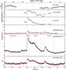 |
Fig. 1 Light curves of AB Dor A observed on 25 Nov. 2009: a) 5.5 GHz radio flux from ATCA observations binned to 120 s; b) and c) Ca ii K flux and Hα equivalent widths calculated from UVES spectra; d) OM light curve; e) EPIC (combined MOS and pn) light curve; f) EPIC hardness ratio. Light curves d) to f) are binned to 100 s. The vertical lines in panel e) indicate the time segment corresponding to the events discussed in the article. Plotted at the top is the arbitrary rotation phase. |
In Fig. 1 we provide a summary of our observations
carried out as a multi-wavelength campaign designed to cover the coronal and chromospheric
properties of AB Dor A. Starting from the top in Fig. 1, we plot the radio light curve recorded at 5.5 GHz with 120 s binning (panel a).
The 9.0 GHz light curve is not shown, since it is very similar to the 5.5 GHz light curve.
In Figs. 1b and c, we show the measured UVES Ca ii
K and Hα equivalent widths (EW) as two examples of strong
chromospheric emission lines, which originate in the lower and upper chromospheres,
respectively. In Figs. 1d and e, we plot the
XMM-Newton OM and EPIC (pn and MOS combined) light curves with a binning
of 100s. To identify heating events, we define a hardness ratio (HR) for the EPIC-pn as
 ,
where H is the number of counts between 1.0 and 10.0 keV (hard band), and
S the number of counts between 0.15 and 1.0 keV (soft band), and plot the
time-dependent hardness ratios (HR) in Fig. 1f. The
most extensive data set comes from XMM-Newton, which observed AB Dor for a
total of 16 h contiguously (from Nov. 25, 21:00 to Nov. 26, 13:00). UVES data are available
for the time span between Nov. 26, 2:00 to 9:30, radio data is available from Nov. 25,
21:00–24:00 UT and Nov. 26, 6:00–13:00 UT.
,
where H is the number of counts between 1.0 and 10.0 keV (hard band), and
S the number of counts between 0.15 and 1.0 keV (soft band), and plot the
time-dependent hardness ratios (HR) in Fig. 1f. The
most extensive data set comes from XMM-Newton, which observed AB Dor for a
total of 16 h contiguously (from Nov. 25, 21:00 to Nov. 26, 13:00). UVES data are available
for the time span between Nov. 26, 2:00 to 9:30, radio data is available from Nov. 25,
21:00–24:00 UT and Nov. 26, 6:00–13:00 UT.
The most notable feature in the AB Dor light curve is a large flare or possibly a sequence of flares lasting from about Nov. 26, 3:00–9:00 UT, which was covered by both XMM-Newton and UVES simultaneously, while the major part of the flare was unfortunately missed at radio wavelengths. A rough estimate of the flare energetics is given in Table 1. There are in addition a number of small scale events visible in the XMM-Newton OM and EPIC light curves as can be seen in Fig. 1e; however, we concentrate on the large events in this paper.
Integrated energies of individual flare events in XMM-Newton’s EPIC and OM.
For purposes of discussion we distinguish the following events, which may or may not be physically connected:
-
Event 1: the first and main flare starts at 02:57 UT, marked by a steep flux rise in all covered wavelength bands. Also many chromospheric emission lines go into emission at this instance, e. g. all Balmer lines covered, the Ca ii H and K line, the Na i D lines, and the He i D3 line. The X-ray count rate increased from a quiescent value of ~14 cts/s in the pn and ~5 cts/s in the MOS detector to ~38 cts/s and ~15 cts/s in the pn and MOS detectors, respectively, at flare peak. In the HR we find a clear hardening to ≈− 0.2 during the large flare. The end of Event 1 cannot be defined uniquely since it is overlaid by Event 2. Therefore, we define its end simply as the onset of Event 2.
-
Event 2: the second event has a broad, slowly changing light curve with its onset marked by a small flare-like event at about 3:40 UT in the OM light curve, which coincides with a slope change in the chromospheric and X-ray light curves. The hardness ratio starts to increase again at about the same time. The decay of Event 2 lasts until 6:40 UT, when a short period of constant X-ray count rate starts. The pronounced broad maximum of Event 2 occurring in the X-ray data at about 5:00 UT has no obvious counterpart in the other wavelength bands. In the OM light curve there is again a minor event and the Hα light curve displays a plateau at the time of the X-ray maximum (see Sect. 6.1). From the light curve morphology it is not clear whether Event 2 is associated with Event 1 as a reheating episode or whether it is independent so we pursue this issue further in Sect. 6.
-
Event 3: the third event starts at 07:34 UT and lasts until about 10:00 UT. This event can be traced in the X-ray and OM data and in the chromospheric emission lines. It is the only event with simultaneous coverage at radio wavelengths; however, the radio light curve shows no clear response when compared to the flare data in the other bands.
4. X-ray spectral analysis
In the following section we provide a detailed discussion of our X-ray observations of AB Dor.
4.1. Spectral fits and elemental abundances
4.1.1. Quiescent and flaring emission
The time span before 2:50 UT is free of any large temporal variations, so we define this period as the preflare quiescent state of AB Dor A. The comparison of our EPIC-MOS spectra taken during quiescence and during the flare rise phase shows the expected flare-related changes in the spectral energy distribution, yielding a substantial increase in emission at higher temperature. During a flare, fresh material from the photosphere and chromosphere is brought to the upper layers of the stellar atmosphere, resulting in a temporary change in the coronal abundance.
We therefore performed a detailed X-ray spectral analysis to determine plasma temperatures, emission measures, and abundances for the different activity states of AB Dor A. We specifically determined the abundances relative to solar values (Grevesse & Sauval 1998) with an iterative procedure of global XSPEC fits to EPIC and RGS spectra with VAPEC plasma models. In these fits, the derived abundances and emission measures are inherently interdependent, therefore we make our inferences from the relative changes of the fit parameters derived for the observations.
We compare each of the events introduced in Sect. 3 with the quiescent state using our RGS and EPIC-MOS spectra. We fit each of these spectra in the energy range 0.2–10.0 keV in the following fashion. We first constructed a fixed temperature grid at the grid points 0.3, 0.6, 1.2, and 2.4 keV (~3.5, ~7.0, ~14.0, and ~28.0 MK, respectively). These temperature grids agree with the best fit temperatures obtained by Sanz-Forcada et al. (2003), who analysed three years of XMM-Newton data of AB Dor A. For fitting RGS spectra, the abundance of carbon, nitrogen, oxygen, neon, and iron were allowed to vary independently, but were fixed between all VAPEC temperature components. Meanwhile when fitting EPIC-MOS spectra, the abundances of magnesium, silicon, sulphur, and argon were allowed to vary along with those of oxygen, neon, and iron, but the carbon and nitrogen abundances were fixed to values obtained from RGS, which is sensitive to strong individual lines; the resulting fit parameters for the various states of AB Dor A are given in Table 2. Satisfactory fits (from a statistical point of view) can be obtained. During all the flares a pronounced enhancement of the emission measure at 2.4 keV (28 MK) is present and, to a lesser extent, at the very softest energies. As far as the abundance pattern between flare and quiescent states is concerned, there is no clear difference except for the elements Fe and Ne, which are clearly enhanced during the flaring states.
Fixed 4-temperature grid fit to the quiescent and the flaring states with variable elemental abundances.
4.1.2. FIP effect
The measured abundance patterns of AB Dor A during flare and quiescence are shown in Fig. 2, where we plot the abundances with respect to solar photospheric abundances against the FIP (first ionisation potential) of the corresponding element. Inactive stars like the Sun show the so-called “FIP effect”, where low-FIP elements like Fe, Si, Mg etc. are enhanced in the corona when compared to high-FIP elements like C, N, O, Ne, etc. However, a reverse pattern called the “inverse FIP effect” (IFIP) is observed in active stars (e.g. Brinkman et al. 2001; Audard et al. 2003). As can be seen in Fig. 2, the abundance pattern of AB Dor A for both quiescent and flaring state indicates the inverse FIP effect, which is consistent with the results of Güdel et al. (2001).
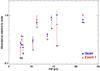 |
Fig. 2 AB Dor A’s coronal abundance relative to solar photospheric values (Grevesse & Sauval 1998) as a function of the first ionisation potential (FIP) during quasi-quiescence (blue) and Event 1 (red). |
4.1.3. Coronal densities
Using our RGS spectra we can investigate the electron densities of the coronal plasma from an analysis of the density-sensitive line ratios of forbidden to inter-combination lines of the helium-like triplets (N vi, O vii, Ne ix, Mg xi, and Si xiii); the theory of density-sensitive lines has been described in detail by Gabriel & Jordan (1969). Only the He-like triplet of O vii is strong enough to be used to obtain the characteristic electron densities in the source region. In Fig. 3 we show the quiescent and flaring RGS spectrum of the O vii triplet, together with the best fits to the triplet lines r (resonance), i (inter-combination), and f (forbidden) provided by the CORA program (Ness & Wichmann 2002). The measured line counts and the deduced f/i ratios are listed in Table 3 for the pre- and post-flare quiescence (integration time of 20 ks and ~10 ks, respectively), the individual and summed flaring events.
X-ray counts measured by best fit to lines and f/i ratios deduced from the O vii triplet.
To convert the measured f/i ratios to electron densities ne, we use the expression
 where
Ro denotes the low density limit and
Nc the critical density and adopted the values of
Ro = 3.95 and
Nc = 3.1 × 1010 cm-3 from Pradhan & Shull (1981). The line ratio errors
are large because of the weakness of the inter-combination line. Since the errors
overlap, there is – formally – no significant change in density. However, the above
density estimates for the flares have not been corrected for any contribution from the
quiescent emission. If the quiescent emission contribution is accounted for in the flare
data, by subtracting the individual line fluxes scaled by the respective exposure times,
then the f/i-ratios decrease
further (cf., 6th row in Table 3). Indeed, the actual
flare plasma densities becomes very high though it should be noted that the associated
measurement errors are even higher.
where
Ro denotes the low density limit and
Nc the critical density and adopted the values of
Ro = 3.95 and
Nc = 3.1 × 1010 cm-3 from Pradhan & Shull (1981). The line ratio errors
are large because of the weakness of the inter-combination line. Since the errors
overlap, there is – formally – no significant change in density. However, the above
density estimates for the flares have not been corrected for any contribution from the
quiescent emission. If the quiescent emission contribution is accounted for in the flare
data, by subtracting the individual line fluxes scaled by the respective exposure times,
then the f/i-ratios decrease
further (cf., 6th row in Table 3). Indeed, the actual
flare plasma densities becomes very high though it should be noted that the associated
measurement errors are even higher.
4.1.4. Emission measure, temperature, and iron abundance evolution
In our previous investigation we only considered the integrated flare spectra. To investigate the variations in temperature, the emission measure, and abundance variations in more detail, we divided the data covering Events 1 to 3 into several time intervals and created X-ray spectra for each of these intervals. The first spectrum covers the flare rise, and the following time intervals cover the different phases of the decay by employing 300 s and 600 s bins so that they contain an approximately equal number of counts per spectrum. Each of these spectra was fitted using a superposition of four-temperature APEC models. Our models always include quiescent emission; i.e., the first two temperature components and its parameters are fixed to plasma properties of the quiescent spectrum before the flare. With this approach, we account for the contribution of the quiescent coronal plasma to the overall X-ray emission. The third and fourth temperature components are allowed to vary freely, but we keep the elemental abundances fixed to quiescent values, except for the iron abundance, which was allowed to vary freely (but of course identical in both the temperature components).
 |
Fig. 3 Density-sensitive He-like triplets of O vii (resonance, inter-combination, and forbidden line for increasing wavelengths) measured with the RGS1 with best fit Lorentzians during preflare quiescence (top) and flaring (bottom) state. Represented as dotted-dashed lines are the three Lorentzians representing r, i and f lines. The continuum close to the triplet is approximated by a straight horizontal line. |
To compare the plasma properties of the two temperature components accounting for the flare, we calculate the “total EM” as the sum of their emission measures and a “flare temperature” as an emission measure-weighted sum of the two temperatures. In Fig. 4, we plot the evolution of the flare temperature, the total emission measure and the Fe abundance. Owing to poor count statistics we end Fig. 4 before the onset of Event 3. The temperature and the emission measure evolution exhibits a decay-like light curve, and the iron abundance also increases from the quiescence level directly before the flare to a maximum during the flare peak (Fig. 4 right panel) and then decreases to preflare values. The increase in Fe abundance around 4:20 UT may not be significant, nevertheless, it coincides with the second peak of the hardness ratio light curve which we define as Event 2 (see Fig. 1). For Event 3 we also checked for iron abundance changes, but because of lower S/N in the data we find no significant change in iron abundance compared to the quiescent state.
 |
Fig. 4 Temporal evolution of flare temperature, emission measure in cm-3 (left panel), and Fe abundance (right panel). Dotted lines indicate the boundaries of each event. |
Clearly, the results in Table 2 suggest that both the Fe and Ne abundances vary significantly. We therefore experimented with various fit strategies and found that the neon abundance does not show a clear pattern like the iron abundance in Fig. 4 (right panel), when it is allowed to vary freely. Furthermore, the fits are only marginally improved, and most of the fit residuals remain unchanged. We also linked Fe and Ne elemental abundances and allowed them to vary freely, but no improvement in the fit quality of the fit was noticed when compared to the fits where only Fe abundance is set free alone. Finally, we repeated the fits treating oxygen, silicon, and their combination as free parameters, but this strategy leads to poorly defined abundances for the individual spectra. Therefore, Fe seems to be the only element that shows a clearly measurable abundance variation during the flare. We cannot exclude the variations of other elemental abundances as well, however, given the spectral resolution and the S/N ratio of our time-resolved X-ray spectra. Such variations – if present – remain hidden in the noise.
4.2. Loop properties
Observations of solar and stellar flares have shown a correlation between the emission measure and the peak flare temperature. The so-called emission measure – temperature (EM–T) diagram has become a useful diagnostic for estimating physical quantities that are not directly observable. By computing EM–T diagrams from specific physical models and comparing and fitting observed and theoretical EM–T curves, one can infer the physical properties of the flare within the chosen model context. With the data from our multi-wavelength campaign, we can assess whether the chosen model is appropriate. Here the model assumes that a stellar flare occurs in a localised coronal region in a simplified geometry (i.e., single loop structure), which remains unchanged during the flare evolution. While the heating is a free parameter in these models, plasma cooling occurs by radiation and thermal conduction back to the chromosphere with their characteristic cooling time scales. These cooling time scales depend on the size of the confining loop structure and on the density of the radiating plasma (Reale et al. 1997). Specifically, Serio et al. (1991) derive a thermodynamic decay time scale of a flare confined to a single flaring coronal loop, by assuming a semicircular loop with a constant cross section, uniformly heated by an initial heating event and without further heating during the decay phase. In this case the loop thermodynamic decay time scale is given by
 where
α = 3.7 × 10⁻⁴
cm-1 s K1/2, T0
(T0,7) is the loop maximum temperature in
units of 107 K, and L (L9) is the
loop half length in units of 109 cm.
where
α = 3.7 × 10⁻⁴
cm-1 s K1/2, T0
(T0,7) is the loop maximum temperature in
units of 107 K, and L (L9) is the
loop half length in units of 109 cm.
To account for further heating during the flare decay, Reale (2007) derived an empirical correction factor by a hydrodynamic simulation
of the loop decay. In this case the loop length can be estimated by the formula
 (1)where
τLC denotes the decay time derived from the light curve.
Here the unitless correction factor F(ζ) describes the
ratio of the observed and the thermodynamic decay time;
F(ζ) is approximated with an analytical function as
(1)where
τLC denotes the decay time derived from the light curve.
Here the unitless correction factor F(ζ) describes the
ratio of the observed and the thermodynamic decay time;
F(ζ) is approximated with an analytical function as
 where
ζ is the slope of the EM–T diagram. The observed peak
temperature must be corrected to
where
ζ is the slope of the EM–T diagram. The observed peak
temperature must be corrected to  (in units
of 107 K), where Tobs is the best-fit peak
temperature derived from spectral fitting to the data. The coefficients
ξ, η, ca,
ζa, and qa depend on the
specific energy response of the instrument used: for XMM/EPIC the appropriate values are
ξ = 0.13, η = 1.16,
ca = 0.51, ζa = 0.35, and
qa = 1.35 (cf. Reale
2007).
(in units
of 107 K), where Tobs is the best-fit peak
temperature derived from spectral fitting to the data. The coefficients
ξ, η, ca,
ζa, and qa depend on the
specific energy response of the instrument used: for XMM/EPIC the appropriate values are
ξ = 0.13, η = 1.16,
ca = 0.51, ζa = 0.35, and
qa = 1.35 (cf. Reale
2007).
We apply Eq. (1) to each of the three
events. We disentangle the events by modelling them assuming an exponential
growth/exponential decay, given by  where CRflare is the count rate at flare peak,
t and tflare are the observation time and
the time of flare peak, respectively.
where CRflare is the count rate at flare peak,
t and tflare are the observation time and
the time of flare peak, respectively.
 |
Fig. 5 Flare evolution in density and temperature for Event 1 (green), Event 2 (blue), and Event 3 (red). |
 |
Fig. 6 Flare onset spectrum of AB Dor A in an arbitrary chosen wavelength range covering the blue end of our observations including the Balmer lines H9–H13. Top: the flare spectrum with a quiescent spectrum subtracted. The identified emission lines are labelled. Bottom: the original flare spectrum. |
In Fig. 5 we show the evolution of the three events in the EM–T plane, which we use to measure the slope ζ of the EM–T evolution. Using these values, the temperatures derived from the spectral fits corrected using the correction factors given in Reale (2007), as well as the decay times derived from the light curve, we can determine the loop half lengths L by using Eq. (1); the input parameters used and the derived loop lengths are provided in Table 4. The length scales listed in Table 4 for Events 1 and 3 suggest that these flaring structures have lengths of 1–2 × 1010 cm2, while the derived loop length for Event 2 is significantly larger. However, this value is presumably overestimated for Event 2 since additional heating seems to occur during its decay. In that case, Event 2 would not comply with the model of a simple, single flaring loop used in the Reale et al. (1997) model.
Decay time τLC derived from the light curve, slopes (ζ) from the EM–T diagram, flare peak temperature T, and deduced loop lengths L for each of the events.
5. Chromospheric properties of AB Dor A
Optical lines, sensitive to chromospheric activity, are found throughout our UVES spectra, most of them in the blue wavelength range up to about 4000 Å. For AB Dor A the strongest chromospheric lines; i.e., the Balmer lines, Ca ii H & K, and Na i D lines also show variations outside of flares, but only during flares do shallow metallic emission lines appear. To illustrate that effect for Event 1, in Fig. 6, we show an arbitrarily chosen wavelength range for both the original recorded spectrum (lower panel) and the net flare spectrum with the quiescent spectrum subtracted. We note that these emission lines can only be recognised in the subtracted spectra in contrast to active mid M-dwarfs, such as Proxima Centauri or CN Leo, where the quiescent continuum in the blue wavelength range is so weak, that the emission lines easily outshine the continuum, especially during flares. Also, the relatively strong photospheric continuum explains why in comparison to these very late-type stars, far fewer emission lines are found in the spectrum of AB Dor A (Fuhrmeister et al. 2008, 2011). Moreover, the high rotational velocity of AB Dor A broadens the lines leading to a lower amplitude, on the other hand, the rotationally broadened lines offer the possibility to identify emission of single active groups, if strong lines show subcomponents.
In the following we first discuss the evolution of strong lines including the absorption features caused by prominences. Moreover, we present an emission line catalogue for Events 1 and 3. Then we concentrate on the analysis of some selected lines.
5.1. Chromospheric line evolution overview
As an example of the development of an emission line throughout our observations we show an intensity map for the Hα and the Ca ii K lines in Fig. 7. For the Hα line we subtracted a PHOENIX spectrum (Teff = 4900 K and log g = 4.5, for more details see below), while we show the original spectrum for the Ca ii K line. The main flare onset can be noted as a bright horizontal line directly before 3:00 UT. For both lines one can see the line broadening directly after flare onset: for the Hα line, there is a significant brightening on the red side up to 6575 Å, while for the Ca ii K line the core is broadened. The Ca ii K line shows its strongest brightening directly at flare onset. In contrast, the Hα line shows the strongest brightening about half an hour later, and it seems to be drifting from blue to red, making it questionable that the brightening is really related to the main flare. Also the third event shows up in the intensity map, starting at about 7:30 UT, directly before the second observation gap and extending to the end of the observations.
Judging from the Hα line and compared to previous observations, AB Dor A is in a state of medium activity during our whole observation. The absorption transients in the original spectra reach a depth of about 0.8–0.85, which seems to be quite typical compared to the findings of Collier Cameron & Robinson (1989) and Vilhu et al. (1991). The latter also detected significant Hα emission in the unsubtracted spectra, which they ascribe to flaring activity or a high density prominence. The flaring activity in our observations does not exhibit such a pronounced Hα emission line, consistent with our X-ray observations, which would also suggest a medium activity state during our observations.
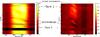 |
Fig. 7 Intensity map of the Hα line (right – with a PHOENIX photospheric spectrum subtracted) and for the Ca ii line (left – original spectrum, no spectrum subtracted). The two horizontal bars indicate observational gaps. |
5.1.1. Crossing prominences
In addition to the brightening events a few dim structures can be noted in the intensity map between 5:00 and 7:30 UT. Such absorption transients are frequently observed in the spectra of AB Dor A and some other highly active stars. These absorption features drift very quickly across the line profiles of the Balmer and Ca ii H&K lines; occasionally, these lines even show such transients in emission. Following early analyses of this phenomenon (Collier Cameron & Robinson 1989) these transients are usually ascribed to clouds of circumstellar material held – at least to a large extent – in co-rotation with the star by strong coronal magnetic fields. Interpreting the drift velocities of these transients as caused by rigid rotation with the stellar surface leads to remarkably large elevations of the putative co-rotating clouds above the stellar surface, reaching heights of up to about five stellar radii or even more (Dunstone et al. 2006; Wolter et al. 2008).
Assuming a stellar inclination of i = 90°, the velocity of a structure
at a distance r from the stellar rotation axis projected onto the line
of sight is given by
vr = ωrsinωt,
where ω denotes the angular velocity of the star. The observed
wavelength of the transient is determined by this velocity, which exceeds the rotational
velocities on the stellar surface. In our case, the curvature of the line profile
transients,  cannot be
determined. As a result, we approximate the above expression to first order.
Differentiation yields
cannot be
determined. As a result, we approximate the above expression to first order.
Differentiation yields  ; and finally, including the
projection due to the stellar inclination, we obtain
; and finally, including the
projection due to the stellar inclination, we obtain  (2)which allows us to
compute the height r for a line profile transient as a function of its
observed “drift velocity”
(2)which allows us to
compute the height r for a line profile transient as a function of its
observed “drift velocity”  through the spectrum. We note that
r − R⋆ is the height
above the stellar surface, only if the absorbing cloud is located in
the equatorial plane. In general, the determined value of
r − R⋆ is a
lower limit to its height. To convert the values of
r into stellar radii, we used the
R⋆ = 0.96 ± 0.06 R⊙,
as determined by Guirado et al. (2011) based on
VLTI/AMBER interferometry in the NIR, and an adopted distance of 14.9 ± 0.1 pc.
through the spectrum. We note that
r − R⋆ is the height
above the stellar surface, only if the absorbing cloud is located in
the equatorial plane. In general, the determined value of
r − R⋆ is a
lower limit to its height. To convert the values of
r into stellar radii, we used the
R⋆ = 0.96 ± 0.06 R⊙,
as determined by Guirado et al. (2011) based on
VLTI/AMBER interferometry in the NIR, and an adopted distance of 14.9 ± 0.1 pc.
As can be seen in Fig. 7, Ca ii K shows sharper transients than Hα. On closer inspection both lines show multiple transients. The properties of the four main transients that could be identified in both lines, Ca ii K and Hα, are listed in Table 5. We give the approximate time for crossing the line centre, so that the prominence can be identified in Fig. 7. Moreover, we list the drift velocity and the height above the stellar surface using an inclination of 60° (Kuerster et al. 1994; Donati et al. 2003).
To quantify the uncertainty of the resulting heights, we estimated the typical error of our determined drift velocities to 15 km s-1/h, i.e. about 10%. The stellar inclination is best determined by Doppler imaging, its precise uncertainty is difficult to assess. Looking at Fig. 3 of Kuerster et al. (1994), it can be determined within a margin of 10 to 15 degrees. This amounts to an uncertainty of about 15% in sini. Plugging these numbers into Eq. (2) and neglecting the small uncertainty of the stellar rotation period, the relative uncertainties of the drift velocity and sini approximately add up to a relative uncertainty of 25% for the resulting prominence radii. A formal error propagation leads to a similar result. Additionally, it should be kept in mind that the heights given in Table 5 are lower limits to the true prominence heights. The actual heights depend on the prominence latitudes which, though apparently close to the equator, are not known in detail.
Properties of the main transients.
In addition to the radial extent of the tentative prominences it would be interesting to estimate their lateral size relative to the stellar disk, following the procedure of Collier Cameron et al. (1990). However, identifying an actual feature belonging to a given transient in the individual line profiles turned out to be cumbersome – owing to the multitude of significant features present in our spectra. Thus, we consider such an analysis beyond the scope of this paper.
We also searched for X-ray absorption features at the prominence crossing times, but could not find any evidence of an X-ray imprint of these features. Using the X-ray data we estimate an upper limit of NH = 9 × 1018 cm-3 to the hydrogen column density of the prominence material. While this number implicitly assumes cosmic abundance for the absorbing material, however, the quoted values are independent of the actual ionisation state of hydrogen.
5.2. Line fitting procedure
In order to quantitatively determine the properties of individual chromospheric emission lines, we performed fits using up to three Gaussian components treating the width σ, the amplitude, and central wavelength as free parameters for each component. Since we are dealing with 460 spectra, the lines were fitted semi-automatically; i.e., we checked the fit quality by eye for each spectrum and line, and if the fit did not reproduce the observed line profile well, we changed starting parameters and/or the fit parameter restrictions. Often the line shapes are quite complicated, such as when the Na i doublet being an absorption line with some filling in, but without any emission core, which leads to poor fits in the context of our simple fitting approach. We checked the possibilities of subtracting either an observed quiescent spectrum or a PHOENIX photospheric model spectrum (Hauschildt et al. 1999). For the latter we determined the best-fitting PHOENIX spectrum for different quiescent spectra of AB Dor A using a model grid with Teff ranging from 4700 to 5200 K in steps of 100 K, with log g ranging from 3.5 to 5.0 in steps of 0.5, and with the rotational velocity ranging from 60 to 120 km s-1 in steps of 10 km s-1 using solar metallicity. Our best fit values are a log g of 4.5, an effective temperature of 4900 ± 100 K, and a projected rotational velocity of 100 ± 10 km s-1, in agreement with the value of 91 km s-1 adopted by Jeffers et al. (2007). The PHOENIX model spectrum describes the photospheric lines quite well in general, although the amplitudes of individual lines differ in many cases.
As individual lines we fitted the Ca ii K line (the H line is too complicated due to blending with Balmer line emission), the Na i doublet at 5889 and 5895 Å, the He i D3 line, Hα, Hβ, Hδ, and, as an example of a shallow metal line, the Si i line at 3905 Å. The Si i and the He i D3 line were both fitted using a running mean; i.e., for each fit, two consecutive spectra were averaged, nevertheless moving through every spectrum.
5.2.1. Observed vs. simulated spectrum as quiescent template
As shown in Fig. 6, a quiescent template spectrum must be subtracted from the flaring spectra in order to identify and properly analyse the flare emission lines. Using a model spectrum or an observed spectrum as quiescent standard has both advantages and disadvantages.
When subtracting a PHOENIX model spectrum, the deviations of the model from the observed photosphere may be as large as the amplitudes of the low amplitude metallic chromospheric emission emerging during the flare. Therefore, a PHOENIX model can only be used for modelling strong emission lines. For these lines the general chromospheric emission leading to the filling-in of the lines (or to emission cores) is often so large that after subtraction of a PHOENIX spectrum, one ends up with a strong emission line, with the flare and emission of single active regions only playing a minor role, which cannot be properly modelled with an automatic fit. This is only possible for the Hα line, where the emission of the flare and individual components is strong enough to show up against the emission core.
Subtracting an observed non-flaring spectrum as a proxy for the quiescent spectrum has the disadvantage that the spectra change significantly on short time scales (about 10 min), with single features of the line moving either in central wavelength or changing in amplitude. For example, in the Hα line, subtracting an average of the first three spectra from each single spectrum, after only about ten minutes of observations an additional emission feature is turning up, and again about ten minutes later, an absorption component manifests itself, but these features are only defined relative to the subtracted averaged spectrum. For example, the absorption feature is caused by the dimming and shifting of a strong emission component in the averaged quiescent spectrum, and therefore not a “real” absorption component. This effect is illustrated for Hα line in Fig. 8, where the PHOENIX subtracted lines are shown and one notes the shifting and dimming. An example of an absorption line caused by changes in the quiescent emission can be found in Fig. 12 in the last two sub-frames. The distributed and fast changing chromospheric emission is also discussed in Sect. 6.5.
 |
Fig. 8 Examples from the evolution of the Hα line after subtracting a PHOENIX spectrum in the first hour of observations, covering the main flare. Blue: spectrum at 2:13 UT (first spectrum taken), green: spectrum at 2:48 UT; red: spectrum at 2:58 UT (flare onset); black: spectrum at 3:05 UT. The additional flux in the black spectrum (best seen at about 6557 and 6570 Å) is caused by the broad line component. |
Nevertheless, for several lines the fitting process is best done using an observed quiescent spectrum. This method gives reliable results for the lines that are not present before the flare or that show up only shortly before the flare (all lines and broad line components except the Balmer lines and the Ca ii K narrow line components).
In the following sections we present our findings from the line fitting.
5.3. Catalogue of emission lines
For Events 1 and 3, a number of chromospheric metal lines besides Ca ii H & K show up in the spectrum. Event 2 does not influence the shallow metal lines. Therefore, we compiled an emission line list for Events 1 and 3. For the line identification we generally used the Moore catalogue (Moore 1972). The line fit parameters – central wavelength, half width, and flux in arbitrary units – and (tentative) identifications including some comments can be found in Table 6. We only show a few rows of this table in the paper as an example, while the whole table is available at the CDS.
5.3.1. Emission line properties
For assessing the metal line properties for Event 1, we averaged the first and second flare spectrum and subtracted an averaged quiescent spectra constructed out of the first three spectra of the night. We identified a total of 90 emission lines in the blue arm and 11 lines in the red arm spectra with a mean wavelength shift of 39.6 ± 9.6 km s-1 (applying a radial velocity of 32.5 km s-1). The rather large scatter is caused by blended lines, for which the probable components are given as a comment in Table 6. Because of the high noise level, the line list cannot be considered complete with respect to weak emission features. Most of the blue emission lines can be detected between 20 and 50 minutes after flare onset. Although Balmer line and Ca ii H and K emission persists for about one hour after flare onset, this emission no longer appear to be flare-related. During Event 3 only 17 emission lines appear, and are a subset of the emission lines found during Event 1. Sufficiently strong lines significantly change in subsequent spectra, even in the relatively weak Event 3. As for Event 1, we took the average of the three spectra directly preceding Event 3 as a proxy for a quiescent spectrum. The lines have an average line shift of − 23.9 ± 13.2 km s-1, which differs by more than 60 km s-1 from the velocity measured for Event 1.
5.3.2. Comparison to other line catalogues
We compared the emission lines found in our AB Dor A spectra to those found in Proxima Centauri by Fuhrmeister et al. (2011), which have an overlapping wavelength region between 3720 and 4485 Å and between 6400 and 9400 Å. We found that most of the lines in the AB Dor A flare coincide with the strongest lines identified in the Proxima Centauri flare. Nevertheless, there are 21 lines in the AB Dor A flare not found in the Proxima Centauri flare (see remarks in the line table). We therefore compare the line list also to the one of the CN Leo mega-flare (Fuhrmeister et al. 2008), where the wavelength overlap is, however, much smaller. In the overlapping line region, all lines not found in the Proxima Centauri list could be identified except for one line.
5.4. Timing behaviour of the strongest lines
The flux in the three strong lines Hα, Hβ, and less pronounced for Ca ii K shows a slow increase and (later on) decrease well before Event 1 (see Fig. 11; the Hα and Ca ii K fluxes peak at about 2:30 UT, while the Hβ flux peaks at about 2:40 UT).
 |
Fig. 9 Spectra of Hα (red), Hβ (green), and Ca ii K (blue) with a PHOENIX spectrum subtracted and scaled for convenience. For comparison the PHOENIX-subtracted flare spectrum (2:58 UT) of each line is over-plotted in black. Different behaviour is seen for the lines, e. g. at 3:14 UT, where the Ca ii line is still double peaked, while in Hα and Hβ the peak at 40 km s-1 has already decayed. Also, the rotationally induced shift of line components is seen, e. g. in Hα the main component, which moves from about –40 (3:14 UT) to +20 (3:41 UT), +30 (3:50 UT), and finally to +50 km s-1 (4:12 UT). |
 |
Fig. 10 Characteristics of the broad line component: Top: flux amplitude; Middle: velocity shift of the line centre; Bottom: Gaussian width in km s-1. The legend applies to all panels. The earlier rise in the He i D3 line is caused by using a running mean for the fitting process. The high velocity shifts in Hα are caused by line subcomponents influencing the fit. The vertical bar in each panel represents a typical error bar. |
A time series comparing the cores of the three strongest lines with a PHOENIX spectrum subtracted is shown in Fig. 9, where the lines are scaled for convenience. The lines in the spectrum taken at 2:22 UT show a single-peaked line centre, that decays and develops a double-peaked structure before the flare for all three lines with one peak at about 40 to 45 km s-1 and a second broader and shallower peak at about –80 km s-1 for the Hα and Hβ lines and about –50 km s-1 for the Ca ii K line. This large difference in velocity cannot be explained only by different line-forming heights and remains unexplained. This second peak can be seen at 6561 Å in Fig. 8 for the Hα line in the green spectrum taken at 2:48 UT. Also it shows up in the flare spectrum in Fig. 9, since the blue peak is nearly undisturbed by the flare. The blue feature is migrating red-wards until it reaches 40–50 km s-1 at about 4:10 UT (see Fig. 9 or 7). We interpret the blue peak as the signature of an active region rotating into view.
Event 1 occurred in the red-shifted half of the line, while the blue emission peak is nearly undisturbed. After Event 1, for Hα and Hβ, the line flux in the flaring component decays rapidly below the flare onset amplitude, while for the Ca ii K line, the amplitude stays at the level of flare onset (see Fig. 9, 3:14 UT). This indicates that the heating of the flare site diminishes in the upper chromosphere, while in the lower chromosphere the heating persists. This state persists for about 40 min during which the blue-shifted component brightens considerably and shifts red-ward with a drift velocity of about 90 km s-1 per hour and eventually reaches the about 50 km s-1 of the original flare site at the stage it also reaches maximum brightness (about 3:47 UT). In Fig. 9 this corresponds to the peaks seen in Hα and Ca ii K starting at flare peak at about –70 (–50 for Ca ii K) km s-1, seen at 3:14 UT at about –40 km s-1, at 3:41 UT (and 3:50 UT) the peak reaches about 40 km s-1. This drift is seen better in the shift of the fitted Gauss kernels for the lines. This brightest episode in Hα at about 3:45 UT can also be noted in the intensity map and coincides with the onset of Event 2. Furthermore, another active region rotates into view in the blue line wing, which can be seen in the spectrum taken at 4:12 UT (Fig. 9). The difference between Hα and Hβ (the Hα amplitude is similar to the one during the flare, while the amplitude of Hβ is well below the flare values) might be explained by a different optical depth of the two lines. While both components decay further for Hα and Hβ, the blue component of the Ca ii K line brightens until about the spectrum taken at 4:45 UT, which again indicates the different heating at different heights.
In the following we discuss the behaviour of the lines during Event 1 in more detail.
5.4.1. Broad line components
During Event 1 the Balmer lines, He i D3, as well as the Ca ii H and K lines, show a very broad component, whose velocities and lifetimes differ significantly from the narrow components. For the He i lines at 3819.6, 4026.2, and 6678.1 Å the line amplitudes are not strong enough to reveal a broad component, although the latter at least shows a second component. These broad component has been noted mostly in M-dwarf flares (Crespo-Chacón et al. 2006; Fuhrmeister et al. 2008, 2011), but also for young K-dwarfs (Montes et al. 1999 and references therein). They can be blue- or (more often) red-shifted, and are often ascribed to a moving turbulent plasma component. Broadening, especially of hydrogen lines, may also be caused by the Stark effect; for a flare on Barnard’s star, Paulson et al. (2006) attributed a symmetric line broadening to the Stark effect. Also, for the Sun Johns-Krull et al. (1997) found evidence of Stark broadening in higher order Balmer lines during a strong flare.
In Fig. 10 we show the results of our Gaussian fit to the broad component of the lines discussed above. Since individual errors would clutter up the graphs, we only give typical error bars for our measurements. All broad line components exhibit red shifts and no blue shifts. The higher shift of the Hα line that starts a few minutes after flare onset is most probably caused by additional red-shifted narrow line components, which are not included in our model but influence the fit of the broad component (see Fig. 12).
The fluxes of the Ca ii K and the He i D3 line peak later and more gradually than the Balmer lines. For the Ca ii K line the observed behaviour could be explained by a height effect and corresponds directly to the behaviour of the main component (see below). For the He i D3 line the broad component is shallow and therefore noisy, which may hide a true peak directly after the flare onset. The earlier flare onset for this line is an artefact of the running mean used for the fitting and not of physical origin. The broad component vanishes about an hour after flare onset as illustrated by the decaying line flux seen in Fig. 10.
5.4.2. Stark broadening versus turbulent broadening
Although the uncertainties of the fit parameters for a our Gaussian line components are rather large – as indicated by the scatter of the measurements – we can discern Stark broadening from turbulent broadening in our data. As seen in Fig. 10, there is a clear trend towards Balmer line widths being larger than the widths of the helium and Ca ii K lines from flare onset until about 3:10 UT. We ascribe this difference to Stark broadening. For a notable Stark broadening of helium lines, very high densities of at least 1016 cm-3 would have to be reached (Ben Chaouacha et al. 2007), which is not expected for this rather small flare. Therefore we argue that the broadening observed in the He i D3 and Ca ii K is turbulent broadening, while the additional broadening observed in the Balmer lines is caused by Stark broadening.
We note that Stark broadening should affect higher members of the Balmer series more strongly (Švestka 1972; Worden et al. 1984). While Hβ is as broad as or even broader than Hα, this is not found for the Hδ line. However, the S/N of the spectra is decreasing towards the blue as is the amplitude of the Balmer lines with increasing order. Therefore, even broader tails may be hidden in the noise. For even higher members of the Balmer series, it is not clear whether their broad line components start to merge. Moreover, Paulson et al. (2006) also found less broadening in higher Balmer lines and gave NLTE effects as a possible reason, which affect low order lines most.
Although Stark broadening is present in the Balmer lines, we choose to fit the lines with two or three Gaussian components, instead of a Voigt profile. Asymmetric Stark profiles are expected for moving plasmas, but would have to be calculated with a full 3D hydrodynamic and radiative transfer code, as done by Allred et al. (2006) but is beyond the scope of this work. To obtain estimates of the velocities of the plasma movements a Gaussian approximation should be sufficient.
 |
Fig. 11 Amplitude of the Gaussian fit for the strongest chromospheric emission lines. In case of multiple line components, the strongest narrow fitting component is shown (Hα, Hβ, Ca ii K). The time interval covers the first 2.3 h of observations, including the flare onset at 2:58 UT. For fitting Hα, a PHOENIX spectrum has been subtracted; the change of the green hue indicates that the fit switched to another line component (see text). Colours are indicated in the legend; both Na i D lines are denoted in red. |
 |
Fig. 12 Fit examples of the Hα line with the observed quiescent spectrum subtracted. The data is shown in grey, the fit components are shown in green, blue, and red, and the resulting fit is shown in black. The data contains additional narrow short-lived line components, which are not fitted here, but are indicated by arrows for the two most complicated spectra at 3:59 UT. Between 3:00 and 3:01 UT the fit switches to another line component. The second spectrum in the upper row shows the flare onset. In the last two spectra one can note an absorption line at about 6563 Å, which is caused by the dimming of a preflare line component and not caused by the flare. |
5.4.3. Narrow line component
The evolution of the flux of the main narrow line emission component is shown in Fig. 11. The Hα line is fitted after subtracting a PHOENIX spectrum and scaled by 0.43, while all other lines were fitted using a quiescent spectrum of AB Dor A for subtraction. Also, since the Hα line displays more than one narrow component, the fit switches to another component directly after flare onset, which is marked in Fig. 11. Also, the dip between 3.5 and 4.0 UT in Hα flux is not real but is caused by the fit shuffling flux from one to another fit component (the total Hα flux peaks at about 3.75 UT).
5.4.4. Subcomponents of the Hα line
We also searched for weaker subcomponents in the Hα line. As discussed in Sect. 5.2.1 they are more pronounced, when subtracting a quiescent spectrum of the star instead of a PHOENIX spectrum. Figure 12 shows the evolution of the Hα line only during a few minutes around flare onset; for all panels, the averaged spectrum taken between 2:56 and 2:58 UT has been subtracted as a proxy for the quiescent state. The figure nicely illustrates the complex and rapidly evolving multi-component structure of the chromospheric emission during the impulsive phase of the flare. Obviously, for most spectra a fit with only three components is not sufficient to cover all components. However, a fit with four or more components is even more unstable than a fit with three components and can usually not be constrained by the data. In addition to the main flaring component, there are several short-lived and a few longer lived narrow components of which the bluest at about 6561 Å is growing stronger during the decay of the flare. At 3:05 UT, about ten minutes after flare onset, an absorption component appears to emerge. However, it is most likely not caused by the flare, but results from changes in the non-flaring line components relative to the preflare state. On the other hand, we argue that the subcomponents in the Hα line, appearing during the first few minutes of the large flare, are real, since notable changes in the non-flaring spectrum seem to appear on time scales of about ten minutes, while during the flare the development of line features (appearing, shifting, and disappearing) takes place on much shorter time scales.
We interpret these weak subcomponents of the Hα line as signatures of shock waves in the chromosphere. Alternatively they could be small dense “blobs” created during the flare, moving at high intrinsic velocities. Some of them can only be identified in one or two consecutive spectra, translating into a lifetime of one to two minutes. We counted up to six such subcomponents in a single spectrum (2:59 UT, two spectra after flare onset), moving with velocities ranging from –270 km s-1 to +260 km s-1. If these subcomponents are present in more than one spectrum, they normally decelerate; i.e., blue-shifted features shift red wards, while red-shifted features show a drift to bluer wavelengths. This strengthens our confidence that these features are not artefacts and are really caused by the flaring material. The only other line besides Hα with a strong enough S/N level to identify subcomponents is the Ca ii K line. There we find a comparable number of subcomponents, but we cannot identify any of the Ca ii subcomponents with Hα subcomponents even for the stronger ones. This is caused partly by the different velocity scatter ranging from –390 to +190 km s-1. Actually, this is not surprising, if these subcomponents are indeed tracers of material of different temperature potentially at different heights of the atmosphere.
6. Discussion
6.1. Comparison between X-ray and optical signatures
During our 58 ks exposure of XMM-Newton three medium-sized flares occurred within a time interval of only six hours, while the remaining light curve showed no major flux enhancement. In the same time interval the OM light curve also shows larger flux variations, coinciding with the X-ray events. The chromospheric emission lines show more complex flux variations, but it is certainly correct to assume that the different wavelength bands actually trace the same events in different parts of the atmosphere. Furthermore, the question arises whether the three events originate in the same loop or arcade. In the following we discuss these issues for each of the three events.
6.1.1. Event 1
Comparing the X-ray and optical/UV light curves around the main flare onset, we found strong evidence of the Neupert effect. The chromospheric emission lines also reacted and peaked at 2:58 UT, while the X-ray emission peaked later at 3:16 UT. The time integral emission due to accelerated particles (like Hα emission, white-light emission) resembled the rise of the flare light curve in the soft X-rays, a phenomenon denoted as the Neupert effect. In Fig. 13, we plot the time derivative of the soft X-ray light curve (using only EPIC data) and the optical light curve. Since there is no OM data available during the flare rise we construct an optical light curve using the UVES continuum spectra between the wavelengths 3895–3920 Å. We note that during flare rise the derivative of the X-ray light curve matches the shape of the optical light curve; it is also obvious that the optical/UV peak precedes the X-ray peak (see Fig. 13).
The chromospheric lines do not react strongly to the flare in amplitude. In contrast to the X-ray and optical/UV light curve, they show even stronger emission before and after the flare events; i.e., the flare does not dominate the chromospheric line emission. Despite the weak reaction of the chromospheric lines in amplitude, the strong lines do show turbulent broadening, the Balmer lines even show Stark broadening and, on top of that, in the Hα line profile single short-lived shock-like events can be identified. All this is accumulating evidence that the above-mentioned picture of a flare affecting different atmospheric layers is certainly correct for this event.
6.1.2. Event 2
Event 2 has its onset at 3:40 UT and its broad X-ray maximum between about 4:20 and 4:50 UT followed by a slow decay until about 6:00 UT. While the onset coincides with the brightest episode in Hα-emission, the broad X-ray maximum has no clear counterpart in the chromospheric lines. Between about 4:15 and 4:45 UT, there is a slight brightening in one of the Hα-components at a velocity of about –35 km s-1, see Fig. 9. This brightening is not strong enough to be noticed in the intensity map of Fig. 7 or in the main line component analysed in Fig. 11. It is most pronounced in the Ca ii K line, where it even shows up in the intensity map as a slight brightening. As an example, we show the central part of the Ca ii K line covering the times of interest in Fig. 14. The feature is not seen in Hβ, which may be due to the noise level in this line.
Because of the slow rise and decay of the peaks in the X-ray and the chromospheric light curves, it is hard to decide, whether this brightening of the chromospheric lines is physically connected to the X-ray brightening. Therefore, the X-ray signal may stem from a reheating event, while in the chromosphere, a different active region undergoes a brightening that only coincides in time with the coronal activity.
6.1.3. Event 3
Event 3 is characterised by a peak at 7:46 UT in X-rays, starting at 7:34 and lasting until 8:16 UT. Unfortunately, the third flare partly falls in a gap of the UVES observations. Nevertheless, the flare onset is covered and observed at about 7:34 UT, both, in the OM and in the chromospheric emission lines. The chromospheric emission lines all show a rather weak reaction compared to X-rays and the OM. They exhibit a very broad peak with the Na i D lines showing increasing flux until the end of the observations at about 9:20 UT. Ca ii K peaks at about 9:00 UT, while Hα appears to peak during the observational gap.
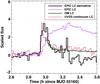 |
Fig. 13 Neupert effect observed during the large flare on AB Dor A. Depicted are the combined EPIC X-ray light curve in violet, its time derivative (smoothed by five bins) in black, the OM light curve in green, and the UVES continuum light curve in red. |
 |
Fig. 14 Central part of the Ca ii K emission line for different times. The spectra are offset for convenience, and a PHOENIX spectrum has been subtracted. The spectrum taken at 4:28 UT is always over-plotted for better comparison. |
6.2. Comparison to other works and to the radio data
The timing of different flares for multi-wavelength observations has been extensively discussed by Osten et al. (2005), who compare parallel radio, optical, UV, and X-ray observations for the young flare star EV Lac and found that flares in different wavelength bands need not have counterparts in any other wavelength bands. Also Kundu et al. (1988) found little correlation between radio and X-ray variations on the flare stars UV Cet, EQ Peg, YZ CMi, and AD Leo. While these two studies did not find a strong correlation between different wavelength bands, other studies did. For example, Liefke et al. (2009) in their study of the flare star CN Leo found clear correlations between X-ray emission, chromospheric lines, and the photospheric continuum at least for the larger events, while smaller events were not seen in all wavelength bands.
During Events 1 and 3 all line fluxes, X-ray, optical, and chromospheric, respond to the flare. On the other hand, Event 2 is substantially different: this long-lasting heating event is observed mostly in the X-ray light curve with little, if any, associated variability in the optical light curve (as seen in the OM) and chromospheric line fluxes. Therefore, Event 2 appears to be largely confined to the corona. In agreement with earlier studies, we could not find any correlation between the radio light curve and other wavelength bands. Furthermore, the radio light curve does not show a significant reaction during the prominence crossings.
6.3. Location of the flaring regions
During Event 1 the chromospheric lines listed in Table 6 and the main components of the Balmer lines show a mean velocity shift of 39.6 ± 9.6 km s-1. Most of these lines appear during the flare onset, but the Balmer lines and other strong lines can be identified before the flare as well. These strong lines show a slow velocity drift over a long time interval, but no abrupt change in their velocity at the onset of Event 1 as can be seen in Fig. 15 for a time interval extending well into flare Event 2. This suggests that the projected rotational velocity of the star and not the intrinsic velocity of the flaring material dominates the velocity of the main line component. This interpretation is further supported by observations of slowly rotating M-dwarfs, for which line shifts during flares are normally not observed; for example, Reiners (2009) searched for radial velocity jitter in UVES observations of the M-dwarf CN Leo and found a jitter of below 1 km s-1 even during the observed very large flare. Nevertheless, most of the glitches and jumps visible in Fig. 15 in the Na i D, Ca ii K, and He i D3 lines occur between the onset and maximum of Event 2. Whether they are physically connected to this event is not clear, though.
Under the assumption that the velocity shift in the chromospheric lines is dominated by rotation and that the chromospheric line emission originates in a region very close to the stellar surface, one can try to locate the flaring active region. Using an inclination of 60° of the stellar rotational axis (Kuerster et al. 1994; Donati & Collier Cameron 1997) and 90 km s-1 as projected rotational velocity, the active region would be about 25° off the centre of the stellar disk in longitude, if located at the equator, and at about longitude of 60°, if located at 60° latitude. Thus, the possibility of the flaring active region being circumpolar (i.e., visible throughout the full rotation cycle) is excluded on the grounds that there are no reversals in the observed velocity shifts (see Fig. 15). However, we note that a small velocity shift reversal could be masked by the changing components of the emission lines during the flare.
 |
Fig. 15 Velocity shift of strong emission lines: Ca ii K (main component, red), Hβ (main component, blue), He i D3 (magenta), and Na i D (two components, rendered green and yellow). Grey and black indicate less reliable sections of the Hβ curve. The graphs of Ca ii K and He i D3 are truncated after about 4:20 UT because of the large scatter of the measurements. |
To constrain the location of the active region further in latitude, we computed the times when the flare would still be visible for different latitudes. However, for the 45-min flare duration (the time span for which the metal lines and the broad line component can be identified), only latitudes lower than about –30° are excluded. As another approach, we measured the drift velocity, i.e. the slope of the velocity shift in Fig. 15, of the lines to be about 20 km s-1 h-1 during Event 1 and large parts of Event 2. This drift velocity implies a latitude of about 60°. However, the highest possible velocity for this latitude on the surface of the star is about 45 km s-1, which is significantly exceeded by the measured velocities reaching about 70 km s-1, see Fig. 15. A possible solution would be to locate the flaring region at some distance from the stellar surface, but distances up to one stellar radius also do not give consistent results, so there seems to be some inconsistency in the drift velocity, which may be influenced to some extent by the line profiles. Thus in summary, we cannot consistently locate the active region responsible for Event 1.
Although the physical connection between the chromospheric and coronal activity is unclear for Event 2, we try to locate the chromospheric active region. To complicate the situation even more, the measured velocities of the chromospheric material at the onset (40–50 km s-1) and the maximum (–35 km s-1) of Event 2 differ substantially, suggesting that the emission may not originate in the same active region. For Event 3 the measured velocity is –24 km s-1. These velocities, together with the rotational drift of the lines, suggest there is no common origin of the different events. This would only be possible for a circumpolar active region, a case excluded above. For instance, Event 2 may even be a superposition of smaller chromospheric brightenings in different regions. Also the intensity map in Fig. 7 suggests different active regions for the Events 1 to 3. Therefore, the simple scenario of a reheating or flares in different arcades of the same active region does not seem to be justified despite the close succession of the three events.
6.4. Geometry of the flaring region
The continuum of the flare optical spectra shows a well-defined slope, suggesting a black-body origin. To compute the black body temperature we use the flare spectrum with the quiescent flux subtracted. The black body fit gives a temperature estimate of 16 000 K during the flare peak. Figure 16 shows the best-fit blackbodies and black body fits with fixed temperatures at 14 500 K and 17 500 K for comparison.
Using the UV light curve obtained with the OM, the optical filling factor can be estimated. For the OM we find a mean count rate of 70 cts/s during the quiescent phase between 21:00 UT and 01:00 UT. Additionally, we obtain the count rate of 190 cts/s at the flare peak (Event 1). Using the count-to-energy conversion factor of 1.66 × 10⁻¹⁵ erg/cm2/s for a star of spectral type K0 from the XMM-Newton handbook, we calculated a flux of 1.1 × 10⁻¹³ erg/cm2/s and 3.1 × 10⁻¹³ erg/cm2/s during quiescent and Event 1 in the covered band of the UVM2 filter. Combining this flux with a distance of ≈15 pc, we obtain a luminosity of 3.2 × 1027 erg/s and 8.6 × 1027 erg/s during quiescent and flare Event 1, respectively. Using the derived temperature and the ratio of flare luminosity to the quiescent luminosity, an area filling-factor of the flare of ≈2.3% can be estimated.
 |
Fig. 16 Blue UVES spectrum with the quiescent flux subtracted, covering the peak of flare Event 1. Overlaid in green and red are different black-body fits. |
Furthermore, one can attempt to estimate the volume of the flaring region in X-rays
making use of the emission measure that is defined by
 , where
ne is the electron density. Using the EM of the hottest
component from Table 2 and
ne from Table 3, we
computed their loop-foot point area
, where
ne is the electron density. Using the EM of the hottest
component from Table 2 and
ne from Table 3, we
computed their loop-foot point area  , where
L is the loop length from Table 4. The resulting filling factor of each of the flaring events range between
1–3%, which is consistent with the estimate from the UV emission.
, where
L is the loop length from Table 4. The resulting filling factor of each of the flaring events range between
1–3%, which is consistent with the estimate from the UV emission.
6.5. Quasi-quiescence in the chromospheric lines
As discussed in Sect. 5.2.1, throughout our observations we find significant variations in line shape and amplitude in Hα, Hβ, and the Ca ii K lines on a time scale of ten minutes and less. These strong chromospheric lines also exhibit subcomponents in their cores. This indicates that they trace emission from different active regions, which are partially resolved in wavelength owing to the high rotational velocity of AB Dor A. The line emission thus results from the superposition of fluxes emitted by the different active regions on the stellar surface. The flux of the different active regions vary in time due to small flares and therefore lead to the very dynamic line behaviour. While the line shape is mostly affected by this phenomenon, even the overall fluxes of the strong lines vary outside the flare events as can be seen in Fig. 7. This is comparable to the situation in X-rays, where many active flare stars do not exhibit a truly quiescent emission level, but some sort of flickering, sometimes called quasi-quiescence (Robrade & Schmitt 2005). Moreover, the chromospheric emission in the strong lines is dominated by many active regions and not by the narrower component emission of the flare. Especially in the Hα-line the flare emission only plays a minor role compared to the overall signal.
6.6. Rotational modulation
Our observations cover about 16 h, translating into ≈1.3 stellar rotation periods. Furthermore, an analysis of rotational modulation in our data is hampered by the fact that a large part of it is highly influenced by flares. Visual inspection of the radio and X-ray light curves suggests that AB Dor A’s emission is rotationally modulated outside Events 1 to 3, see Fig. 1. However, closer inspection shows that the estimated maxima of the radio emission do not match the rotation period of 0.52 d by an hour or more. The same applies to the minima of the X-ray signal. Thus we conclude that we do not see any significant rotational modulation during our observations.
7. Summary and conclusions
The data set reported in this paper contains – to the best of our knowledge – the most comprehensive multi-wavelength data set on the ultra-fast rotator AB Dor A. These data allow us to study temporal correlations of the star’s magnetic activity with unprecedented accuracy. We focused on long duration flare events that were simultaneously covered both in the optical and X-ray domains with very high spectral and temporal resolution. The X-ray data allow determining the coronal abundances, temperature, emission measure, and densities during the different states of activity. The recorded X-ray flare light curve shows a striking similarity to the flares observed previously on the same star described by Güdel et al. (2001).
These clustered events suggest that they originate in the same loop or arcade as to what is observed on the Sun (see Kołomański 2007 and their references); however, our simultaneously recorded high resolution optical data clearly show that these events must have originated in different active regions at least at the chromospheric level. For Events 1 and 3 we do have clear counterparts in the different wavelength bands except for the radio emission that is not covered and that exhibits no flaring activity. On the other hand, a physical connection between the re-heating like Event 2 in X-rays, and the coinciding event in the chromospheric lines is not clear. Additionally, we have found – as in previous observations – strong prominence-like absorptions in the chromospheric line profiles; however, we find no evidence for any X-ray absorption effects by these prominences. Furthermore, no signs of rotational modulation either in X-ray or in radio emission were found in our data.
In our high time-cadence spectral series, we could identify shallow emission subcomponents in the Hα and Ca ii K lines during the first few minutes of the large flare, which we interpreted as the signature of the strongest chromospheric shocks caused by the flare. Moreover, for the first time to our knowledge, we could show that during the early phase of a large flare both turbulent broadening for the helium and metal lines and Stark broadening for the hydrogen lines is at work, but later on only turbulent broadening seems to be present. The presence of Stark broadening in the Balmer lines demonstrates that the flaring region exhibits high densities at the chromospheric level, as expected, in the context of a evaporation scenario, and the same applies to the X-ray emitting plasma, which also shows quite high density. The filling factors derived both from the chromosphere and corona agree and suggest a flaring region covering up to a few percent of the stellar surface, i.e., of the order of a 1–2 × 1010 cm, in agreement with simple estimates derived from hydrodynamic loop models. Our findings demonstrate the extreme complexity of the flare phenomenon and the importance of both high time-cadence and spectral resolution for stellar flare studies.
A detailed description of the UVES spectrograph is available at http://www.eso.org/instruments/uves/doc/
The UVES pipeline manual can be found at ftp://ftp.eso.org/pub/dfs/pipelines/uves/uves-pipeline-manual-13.0.pdf
A detailed description of the instruments on board XMM-Newton is available at http://xmm.esac.esa.int/external/xmm_user_support/documentation/technical/
The XMM-Newton SAS user guide can be found at http://xmm.esac.esa.int/external/xmm_user_support/documentation/
Acknowledgments
S.L. acknowledges funding by the DFG in the framework of RTG 1351. We thank Dr. Stefan Czesla for fruitful discussions.
References
- Allred, J. C., Hawley, S. L., Abbett, W. P., & Carlsson, M. 2006, ApJ, 644, 484 [NASA ADS] [CrossRef] [Google Scholar]
- Arnaud, K. A. 1996, in Astronomical Data Analysis Software and Systems V, eds. G. H. Jacoby, & J. Barnes, ASP Conf. Ser., 101, 17 [Google Scholar]
- Audard, M., Güdel, M., Sres, A., Raassen, A. J. J., & Mewe, R. 2003, A&A, 398, 1137 [NASA ADS] [CrossRef] [EDP Sciences] [Google Scholar]
- Beck, C., Schmidt, W., Rezaei, R., & Rammacher, W. 2008, A&A, 479, 213 [NASA ADS] [CrossRef] [EDP Sciences] [Google Scholar]
- Ben Chaouacha, H., Sahal-Bréchot, S., & Ben Nessib, N. 2007, A&A, 465, 651 [NASA ADS] [CrossRef] [EDP Sciences] [Google Scholar]
- Brinkman, A. C., Behar, E., Güdel, M., et al. 2001, A&A, 365, L324 [NASA ADS] [CrossRef] [EDP Sciences] [Google Scholar]
- Close, L. M., Lenzen, R., Guirado, J. C., et al. 2005, Nature, 433, 286 [NASA ADS] [CrossRef] [PubMed] [Google Scholar]
- Close, L. M., Thatte, N., Nielsen, E. L., et al. 2007, ApJ, 665, 736 [NASA ADS] [CrossRef] [Google Scholar]
- Clough, S. A., Iacono, M. J., & Moncet, J.-L. 1992, J. Geophys. Res., 97, 15761 [NASA ADS] [CrossRef] [Google Scholar]
- Collier Cameron, A., & Robinson, R. D. 1989, MNRAS, 236, 57 [NASA ADS] [CrossRef] [Google Scholar]
- Collier Cameron, A., Duncan, D. K., Ehrenfreund, P., et al. 1990, MNRAS, 247, 415 [NASA ADS] [Google Scholar]
- Crespo-Chacón, I., Montes, D., García-Alvarez, D., et al. 2006, A&A, 452, 987 [NASA ADS] [CrossRef] [EDP Sciences] [Google Scholar]
- Donati, J.-F., & Collier Cameron, A. 1997, MNRAS, 291, 1 [NASA ADS] [CrossRef] [Google Scholar]
- Donati, J.-F., Collier Cameron, A., Semel, M., et al. 2003, MNRAS, 345, 1145 [NASA ADS] [CrossRef] [Google Scholar]
- Dunstone, N. J., Collier Cameron, A., Barnes, J. R., & Jardine, M. 2006, MNRAS, 373, 1308 [NASA ADS] [CrossRef] [Google Scholar]
- Fletcher, L., Dennis, B. R., Hudson, H. S., et al. 2011, Space Sci. Rev., 159, 19 [NASA ADS] [CrossRef] [Google Scholar]
- Fossum, A., & Carlsson, M. 2005, Nature, 435, 919 [NASA ADS] [CrossRef] [PubMed] [Google Scholar]
- Fuhrmeister, B., Liefke, C., Schmitt, J. H. M. M., & Reiners, A. 2008, A&A, 487, 293 [NASA ADS] [CrossRef] [EDP Sciences] [Google Scholar]
- Fuhrmeister, B., Lalitha, S., Poppenhaeger, K., et al. 2011, A&A, 534, A133 [NASA ADS] [CrossRef] [EDP Sciences] [Google Scholar]
- Gabriel, A. H., & Jordan, C. 1969, MNRAS, 145, 241 [NASA ADS] [CrossRef] [Google Scholar]
- García-Alvarez, D., Drake, J. J., Kashyap, V. L., Lin, L., & Ball, B. 2008, ApJ, 679, 1509 [NASA ADS] [CrossRef] [Google Scholar]
- Grevesse, N., & Sauval, A. J. 1998, Space Sci. Rev., 85, 161 [NASA ADS] [CrossRef] [Google Scholar]
- Güdel, M., Audard, M., Briggs, K., et al. 2001, A&A, 365, L336 [NASA ADS] [CrossRef] [EDP Sciences] [Google Scholar]
- Guirado, J. C., Marcaide, J. M., Martí-Vidal, I., et al. 2011, A&A, 533, A106 [NASA ADS] [CrossRef] [EDP Sciences] [Google Scholar]
- Hauschildt, P. H., Allard, F., & Baron, E. 1999, ApJ, 512, 377 [NASA ADS] [CrossRef] [Google Scholar]
- Hussain, G. A. J., Jardine, M., Donati, J.-F., et al. 2007, MNRAS, 377, 1488 [NASA ADS] [CrossRef] [Google Scholar]
- Innis, J. L., Coates, D. W., & Thompson, K. 1988, MNRAS, 233, 887 [NASA ADS] [Google Scholar]
- Jeffers, S. V., Donati, J.-F., & Collier Cameron, A. 2007, MNRAS, 375, 567 [NASA ADS] [CrossRef] [Google Scholar]
- Johns-Krull, C. M., Hawley, S. L., Basri, G., & Valenti, J. A. 1997, ApJS, 112, 221 [NASA ADS] [CrossRef] [Google Scholar]
- Kołomański, S. 2007, A&A, 465, 1021 [NASA ADS] [CrossRef] [EDP Sciences] [Google Scholar]
- Kowalski, A. F., Hawley, S. L., Holtzman, J. A., Wisniewski, J. P., & Hilton, E. J. 2010, ApJ, 714, L98 [NASA ADS] [CrossRef] [Google Scholar]
- Kuerster, M., Schmitt, J. H. M. M., & Cutispoto, G. 1994, A&A, 289, 899 [NASA ADS] [Google Scholar]
- Kuerster, M., Schmitt, J. H. M. M., Cutispoto, G., & Dennerl, K. 1997, A&A, 320, 831 [NASA ADS] [Google Scholar]
- Kundu, M. R., White, S. M., Jackson, P. D., & Pallavicini, R. 1988, A&A, 195, 159 [Google Scholar]
- Liefke, C., Fuhrmeister, B., & Schmitt, J. H. M. M. 2009, in 15th Cambridge Workshop on Cool Stars, Stellar Systems, and the Sun, ed. E. Stempels, AIP Conf. Ser., 1094, 608 [Google Scholar]
- Lim, J., Nelson, G. J., Castro, C., Kilkenny, D., & van Wyk, F. 1992, ApJ, 388, L27 [NASA ADS] [CrossRef] [Google Scholar]
- Montes, D., Saar, S. H., Collier Cameron, A., & Unruh, Y. C. 1999, MNRAS, 305, 45 [NASA ADS] [CrossRef] [Google Scholar]
- Moore, C. E. 1972, in Nat. Stand. Ref. Data Ser. (Washington D.C.: US Dept. of Commerce), 40 [Google Scholar]
- Ness, J.-U., & Wichmann, R. 2002, Astron. Nachr., 323, 129 [NASA ADS] [CrossRef] [Google Scholar]
- Osten, R. A., Hawley, S. L., Allred, J. C., Johns-Krull, C. M., & Roark, C. 2005, ApJ, 621, 398 [NASA ADS] [CrossRef] [Google Scholar]
- Pakull, M. W. 1981, A&A, 104, 33 [NASA ADS] [Google Scholar]
- Paulson, D. B., Allred, J. C., Anderson, R. B., et al. 2006, PASP, 118, 227 [NASA ADS] [CrossRef] [Google Scholar]
- Phillips, K. J. H., & Dennis, B. R. 2012, ApJ, 748, 52 [NASA ADS] [CrossRef] [Google Scholar]
- Pradhan, A. K., & Shull, J. M. 1981, ApJ, 249, 821 [NASA ADS] [CrossRef] [Google Scholar]
- Reale, F. 2007, A&A, 471, 271 [NASA ADS] [CrossRef] [EDP Sciences] [Google Scholar]
- Reale, F., Betta, R., Peres, G., Serio, S., & McTiernan, J. 1997, A&A, 325, 782 [NASA ADS] [Google Scholar]
- Reiners, A. 2009, A&A, 498, 853 [NASA ADS] [CrossRef] [EDP Sciences] [Google Scholar]
- Robrade, J., & Schmitt, J. H. M. M. 2005, A&A, 435, 1073 [NASA ADS] [CrossRef] [EDP Sciences] [Google Scholar]
- Sanz-Forcada, J., Maggio, A., & Micela, G. 2003, A&A, 408, 1087 [NASA ADS] [CrossRef] [EDP Sciences] [Google Scholar]
- Sault, R. J., Teuben, P. J., & Wright, M. C. H. 1995, in Astronomical Data Analysis Software and Systems IV, eds. R. A. Shaw, H. E. Payne, & J. J. E. Hayes, ASP Conf. Ser., 77, 433 [Google Scholar]
- Serio, S., Reale, F., Jakimiec, J., Sylwester, B., & Sylwester, J. 1991, A&A, 241, 197 [NASA ADS] [Google Scholar]
- Smith, R. K., Brickhouse, N. S., Liedahl, D. A., & Raymond, J. C. 2001, in Spectroscopic Challenges of Photoionized Plasmas, eds. G. Ferland, & D. W. Savin, ASP Conf. Ser., 247, 161 [Google Scholar]
- Švestka, Z. 1972, ARA&A, 10, 1 [NASA ADS] [CrossRef] [Google Scholar]
- Sylwester, J., Lemen, J. R., & Mewe, R. 1984, Nature, 310, 665 [NASA ADS] [CrossRef] [Google Scholar]
- Vilhu, O., & Linsky, J. L. 1987, PASP, 99, 1071 [NASA ADS] [CrossRef] [Google Scholar]
- Vilhu, O., Gustafsson, B., & Walter, F. M. 1991, A&A, 241, 167 [NASA ADS] [Google Scholar]
- Vilhu, O., Tsuru, T., Collier Cameron, A., et al. 1993, A&A, 278, 467 [NASA ADS] [Google Scholar]
- Wedemeyer-Böhm, S., Lagg, A., & Nordlund, Å. 2009, Space Sci. Rev., 144, 317 [NASA ADS] [CrossRef] [Google Scholar]
- Wedemeyer-Böhm, S., Scullion, E., Steiner, O., et al. 2012, Nature, 486, 505 [NASA ADS] [CrossRef] [PubMed] [Google Scholar]
- White, G. L., Jauncey, D. L., Batty, M. J., Peters, W. L., & Gulkis, S. 1988, PASP, 100, 825 [NASA ADS] [CrossRef] [Google Scholar]
- Wilson, W. E., Ferris, R. H., Axtens, P., et al. 2011, MNRAS, 416, 832 [NASA ADS] [CrossRef] [Google Scholar]
- Wolter, U., Robrade, J., Schmitt, J. H. M. M., & Ness, J. U. 2008, A&A, 478, L11 [NASA ADS] [CrossRef] [EDP Sciences] [Google Scholar]
- Worden, S. P., Schneeberger, T. J., Giampapa, M. S., Deluca, E. E., & Cram, L. E. 1984, ApJ, 276, 270 [NASA ADS] [CrossRef] [Google Scholar]
All Tables
Fixed 4-temperature grid fit to the quiescent and the flaring states with variable elemental abundances.
X-ray counts measured by best fit to lines and f/i ratios deduced from the O vii triplet.
Decay time τLC derived from the light curve, slopes (ζ) from the EM–T diagram, flare peak temperature T, and deduced loop lengths L for each of the events.
All Figures
|
Fig. 1 Light curves of AB Dor A observed on 25 Nov. 2009: a) 5.5 GHz radio flux from ATCA observations binned to 120 s; b) and c) Ca ii K flux and Hα equivalent widths calculated from UVES spectra; d) OM light curve; e) EPIC (combined MOS and pn) light curve; f) EPIC hardness ratio. Light curves d) to f) are binned to 100 s. The vertical lines in panel e) indicate the time segment corresponding to the events discussed in the article. Plotted at the top is the arbitrary rotation phase. |
| In the text | |
|
Fig. 2 AB Dor A’s coronal abundance relative to solar photospheric values (Grevesse & Sauval 1998) as a function of the first ionisation potential (FIP) during quasi-quiescence (blue) and Event 1 (red). |
| In the text | |
|
Fig. 3 Density-sensitive He-like triplets of O vii (resonance, inter-combination, and forbidden line for increasing wavelengths) measured with the RGS1 with best fit Lorentzians during preflare quiescence (top) and flaring (bottom) state. Represented as dotted-dashed lines are the three Lorentzians representing r, i and f lines. The continuum close to the triplet is approximated by a straight horizontal line. |
| In the text | |
|
Fig. 4 Temporal evolution of flare temperature, emission measure in cm-3 (left panel), and Fe abundance (right panel). Dotted lines indicate the boundaries of each event. |
| In the text | |
|
Fig. 5 Flare evolution in density and temperature for Event 1 (green), Event 2 (blue), and Event 3 (red). |
| In the text | |
|
Fig. 6 Flare onset spectrum of AB Dor A in an arbitrary chosen wavelength range covering the blue end of our observations including the Balmer lines H9–H13. Top: the flare spectrum with a quiescent spectrum subtracted. The identified emission lines are labelled. Bottom: the original flare spectrum. |
| In the text | |
|
Fig. 7 Intensity map of the Hα line (right – with a PHOENIX photospheric spectrum subtracted) and for the Ca ii line (left – original spectrum, no spectrum subtracted). The two horizontal bars indicate observational gaps. |
| In the text | |
|
Fig. 8 Examples from the evolution of the Hα line after subtracting a PHOENIX spectrum in the first hour of observations, covering the main flare. Blue: spectrum at 2:13 UT (first spectrum taken), green: spectrum at 2:48 UT; red: spectrum at 2:58 UT (flare onset); black: spectrum at 3:05 UT. The additional flux in the black spectrum (best seen at about 6557 and 6570 Å) is caused by the broad line component. |
| In the text | |
|
Fig. 9 Spectra of Hα (red), Hβ (green), and Ca ii K (blue) with a PHOENIX spectrum subtracted and scaled for convenience. For comparison the PHOENIX-subtracted flare spectrum (2:58 UT) of each line is over-plotted in black. Different behaviour is seen for the lines, e. g. at 3:14 UT, where the Ca ii line is still double peaked, while in Hα and Hβ the peak at 40 km s-1 has already decayed. Also, the rotationally induced shift of line components is seen, e. g. in Hα the main component, which moves from about –40 (3:14 UT) to +20 (3:41 UT), +30 (3:50 UT), and finally to +50 km s-1 (4:12 UT). |
| In the text | |
|
Fig. 10 Characteristics of the broad line component: Top: flux amplitude; Middle: velocity shift of the line centre; Bottom: Gaussian width in km s-1. The legend applies to all panels. The earlier rise in the He i D3 line is caused by using a running mean for the fitting process. The high velocity shifts in Hα are caused by line subcomponents influencing the fit. The vertical bar in each panel represents a typical error bar. |
| In the text | |
|
Fig. 11 Amplitude of the Gaussian fit for the strongest chromospheric emission lines. In case of multiple line components, the strongest narrow fitting component is shown (Hα, Hβ, Ca ii K). The time interval covers the first 2.3 h of observations, including the flare onset at 2:58 UT. For fitting Hα, a PHOENIX spectrum has been subtracted; the change of the green hue indicates that the fit switched to another line component (see text). Colours are indicated in the legend; both Na i D lines are denoted in red. |
| In the text | |
|
Fig. 12 Fit examples of the Hα line with the observed quiescent spectrum subtracted. The data is shown in grey, the fit components are shown in green, blue, and red, and the resulting fit is shown in black. The data contains additional narrow short-lived line components, which are not fitted here, but are indicated by arrows for the two most complicated spectra at 3:59 UT. Between 3:00 and 3:01 UT the fit switches to another line component. The second spectrum in the upper row shows the flare onset. In the last two spectra one can note an absorption line at about 6563 Å, which is caused by the dimming of a preflare line component and not caused by the flare. |
| In the text | |
|
Fig. 13 Neupert effect observed during the large flare on AB Dor A. Depicted are the combined EPIC X-ray light curve in violet, its time derivative (smoothed by five bins) in black, the OM light curve in green, and the UVES continuum light curve in red. |
| In the text | |
|
Fig. 14 Central part of the Ca ii K emission line for different times. The spectra are offset for convenience, and a PHOENIX spectrum has been subtracted. The spectrum taken at 4:28 UT is always over-plotted for better comparison. |
| In the text | |
|
Fig. 15 Velocity shift of strong emission lines: Ca ii K (main component, red), Hβ (main component, blue), He i D3 (magenta), and Na i D (two components, rendered green and yellow). Grey and black indicate less reliable sections of the Hβ curve. The graphs of Ca ii K and He i D3 are truncated after about 4:20 UT because of the large scatter of the measurements. |
| In the text | |
|
Fig. 16 Blue UVES spectrum with the quiescent flux subtracted, covering the peak of flare Event 1. Overlaid in green and red are different black-body fits. |
| In the text | |
Current usage metrics show cumulative count of Article Views (full-text article views including HTML views, PDF and ePub downloads, according to the available data) and Abstracts Views on Vision4Press platform.
Data correspond to usage on the plateform after 2015. The current usage metrics is available 48-96 hours after online publication and is updated daily on week days.
Initial download of the metrics may take a while.