| Issue |
A&A
Volume 556, August 2013
|
|
|---|---|---|
| Article Number | A84 | |
| Number of page(s) | 12 | |
| Section | Stellar structure and evolution | |
| DOI | https://doi.org/10.1051/0004-6361/201220651 | |
| Published online | 02 August 2013 | |
The complex behaviour of the microquasar GRS 1915+105 in the ρ class observed with BeppoSAX
III. The hard X-ray delay and limit cycle mapping⋆
1
INFN, Sezione Roma 1, Piazzale A. Moro 2,
00185
Roma,
Italy
2
Dipartimento di Fisica, Università La Sapienza,
Piazzale A. Moro 2,
00185
Roma,
Italy
3
INAF, IASF, Sez. di Palermo, via U. La Malfa 153,
90146
Palermo,
Italy
e-mail:
This email address is being protected from spambots. You need JavaScript enabled to view it.
4
Dipartimento di Fisica, Università di Palermo,
via Archirafi 36, 90123
Palermo,
Italy
5
INAF, IAPS, Sez. di Roma, via Fosso del Cavaliere 100,
00113
Roma,
Italy
6
INAF, Osservatorio Astronomico di Roma,
23807
Monte Porzio Catone,
Italy
7
INAF, Osservatorio Astronomico di Brera,
via E. Bianchi 46, 23807
Merate,
Italy
Received:
29
October
2012
Accepted:
25
April
2013
Abstract
Context. The microquasar GRS1915+105 was observed by BeppoSAX in October 2000 for about ten days while the source was in ρ mode, which is characterized by a quasi-regular type I bursting activity.
Aims. This paper presents a systematic analysis of the delay of the hard and soft X-ray emission at the burst peaks. The lag, also apparent from the comparison of the [1.7–3.4] keV light curves with those in the [6.8–10.2] keV range, is evaluated and studied as a function of time, spectral parameters, and flux.
Methods. We apply the limit cycle mapping technique, using as independent variables the count rate and the mean photon rate. The results using this technique were also cross-checked using a more standard approach with the cross-correlation methods. Data are organized in runs, each relative to a continuous observation interval.
Results. The detected hard-soft delay changes in the course of the pointing from ~3 s to ~10 s and presents a clear correlation with the baseline count rate.
Key words: binaries: close / stars: individual: GRS 1915+105 / X-rays: stars
Table 2 is available in electronic form at http://www.aanda.org
© ESO, 2013
1. Introduction
The various phenomena occurring in accretion disks around black holes (BH) can exhibit complex patterns likely originated by non-linear processes. In the case of the microquasar GRS 1915+105, such complex processes produce a large variety of behaviours, ranging from a rather steady and noisy emission to the occurrence of long recurrent burst series. In two previous papers on GRS 1915+105, we investigated the time evolution of the burst series properties in the so-called ρ class (Belloni et al. 2000) using the data collected in the course of a long pointing of BeppoSAX in October 2000 (Massaro et al. 2010, hereafter Paper I); the results of the spectral analysis were described in Mineo et al. (2012, Paper II).
In these two papers, we introduced the regular and irregular modes of the ρ class on the basis of the stability of the recurrence time of bursts Trec, derived from Fourier and wavelet spectra, and on the multiplicity of pulses. We introduced a synthetic nomenclature useful for classifying the various types of bursting. Fourier periodograms of individual series were classified in three types, namely S, T, and M, according to the occurrence of a single, two, or many prominent peaks, respectively. We defined three stability classes, which were denoted as 0, 1, and 2 and corresponded to a decrease of the fluctuations of the highest power time-scale in the wavelet scalograms. Thus series of the S2 type correspond to the most regular ones, whereas the M0 ones are the most irregular. The entire pointing was divided into three successive intervals identified by a Roman numeral: I (from the start time of the observation to 1.7 × 10⁵ s); II (from this time to 3.8 × 10⁵ s); and III (from 4.0 × 10⁵ s to 6.0 × 10⁵ s). In the interval II, GRS 1915+105 was in the irregular mode, while in the two others it was mainly in the regular one. We observed an increase in the baseline count rate from interval II to interval III; the fractional final increase was ~18% and took place in ~20 ks.
In Paper II, we described the results of a time-resolved spectral analysis that was performed splitting the entire burst cycle into a few segments: the slow leading trail (SLT) from the minimum level to about the half height of the pulse (P) and followed by the fast decaying tail, or FDT, in which the count rate decreases to its minimum. The first two segments were moreover separated into two parts of equal duration, named SLT-1, SLT-2 and P-1, P-2, respectively. Bursts are superimposed onto a baseline level (BL), which showed a step-like increase from interval II to III (Paper I). For clarity’s sake, we report in Table 1 a log of the acronyms and labels used in Paper I and II.
Acronyms and labels used in Paper I and II.
Lags between the hard and soft X-ray emission, hereafter named hard-X delay (HXD), have been observed in GRS 1915+105 and in other X-ray binaries (Uttley et al. 2011; Cassatella et al. 2012). The HXD occurrence was reported since early observations of the ρ class in terms of temperature evolution of the multi-temperature disk black body in the course of the burst (Taam et al. 1997; Paul et al. 1998). Similar changes were also found in the spectral analysis presented in Paper II: the disk kT changed from about 1.1 keV in the SLT to about 1.6 keV in the first segment of the pulse (P1), reaching values above 2 keV in the second segment (P2) and decreasing to P1 values during the FDT. The same temperature evolution was reported by Neilsen et al. (2012) using RXTE observations. On time-scales shorter than 1 s, a hard phase lag of the high-energy component with respect to the low-energy one was observed in GRS 1915+105 and other accreting black hole candidates on the basis of Fourier transforms. Cui (1999) reported for GRS 1915+105 a hard X-ray phase lag associated with the 67 Hz quasi-periodic oscillation and showed the existence of both hard and soft phaselags up to ~1 s. Reig et al. (2000) found that a lag was also present in QPOs at lower frequencies [0.6–8] Hz and that their amplitude is correlated with the frequency, while Muno et al. (2001) indicated the existence of both positive and negative lags, according to X-ray and radio intensity levels; in particular, the phase lag sign changed from positive to negative as radio emission increased. Janiuk & Czerny (2005) considered the same RXTE observations of GRS 1915+105 of Belloni et al. (2000) and, applying a cross-correlation to the energy-selected light curves in the [1.5−6] keV and [6.4−14.6] keV bands, found a delay of ~1 s only in the ρ and κ classes. More recently, Neilsen et al. (2012) in their analysis of ρ class data defined the HXD on the basis of the phase separation between the maxima on folded burst profiles in the two energy ranges [2−5] and [12−45] keV. They found that the phase lags depend on burst multiplicity: double-peaked bursts have significantly longer lags (Δφ = 0.08 ± 0.05) than single-peaked ones (Δφ = 0.02 ± 0.02); we note that the latter result is compatible with a zero lag at one standard deviation. For a typical recurrence time of their data (~64 s), the former lag translates into a time distance of ~4.6 s.
The analysis presented in this paper is devoted to the correlated spectral-timing variations of GRS 1915+105 emission in the ρ class; more specifically, we focus on the analysis of the HXD. We developed specific tools for the study of the spectral-timing behaviour by means of a limit cycle mapping and applied these methods to the investigation of both regular and irregular data series to investigate how the HXD changes across the long BeppoSAX observation. After a brief description of data and the HXD phenomenon, we describe the methods developed for mapping limit cycle behaviour in a suitable parameter space and for estimating the HXD. Then our results are discussed and compared with previous findings. We note that our approach and results will also be useful when comparing the ρ class observed in GRS 1915+105 with other sources showing similar behaviour, and possibly the same underlying physical mechanisms as the newly discovered IGR J170913624 (Altamirano et al. 2011), which exhibits very similar variability patterns.
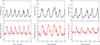 |
Fig. 1 Two 300-s long segments of the count rate (upper panels) and mean photon energy (lower panels) curves of the MECS [1.7–10] keV data series A8b (left), E5 (centre), and F7 (right) after a running average smoothing over five bins. The bin size of all series is 1 s. |
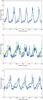 |
Fig. 2 Portions of MECS light curves in the energy ranges [1.3−3.4] keV, green curve, and [6.8–10.2] keV, blue curve. From top to bottom, examples from time interval I (time series A8b), time interval II (E5), and time interval III (F7). The time bin is 1 s. |
2. Observations and data reduction
General descriptions of the long BeppoSAX observation of GRS 1915+105 performed in October 2000 are given in Papers I and II, and we refer to those papers for more details. This observation started on October 20 (MJD 51837.894) and terminated on October 29 after an overall duration of 768.79 ks. In this paper, our analysis is performed only on data obtained with the Medium Energy Concentrator Spectrometer (MECS, Boella et al. 1997) in the energy range [1.7–10] keV, whose statistics are high enough to provide significant information on individual bursts. As shown in Paper I, data at higher energy, as those obtained with the PDS instrument, are noisier and burst features cannot always be clearly established. Data are organized in runs, each relative to a continuous observation interval, and named with letters and sequential numbers. We use the same 52 data series that were already considered in Paper II; they are all within the first 600.725 s of the pointing when the source remained almost stable in the ρ class. The main parameters of the considered runs are given in Table 2.
In addition to the count rate time series, we also consider in the following analysis the
series describing the evolution of the mean energy of photons, which are good for properly
describing the recurring bursting behaviour of the source in a two-dimensional space. These
series were obtained by computing the arithmetic mean ⟨ C ⟩ of the energy
channels assigned to each photon in every time bin and then converting the result with the
instrumental gain relationship  (1)Three
examples of count rate and energy series, which are extracted from the light curves A8b (S2
type, regular), E5 (M0 type, irregular) and F7 (T2 type,
regular), the same already used in Paper I as representative of the
different modes of the ρ class, are shown in Fig. 1. Considering the high scatter of the data due either to statistical
fluctuations or to an intrinsic high-frequency variability, we smoothed the high-frequency
noise by means of a running average filter over a time window of five bins. Curves of the
mean photon energy are generally limited in the quite narrow range between 4.2 keV and 4.8
keV, but their variations are very apparent. Considering that the typical root-mean-squared
(rms) dispersion in each bin is close and generally lower than 0.1 keV, these variations are
significant and consistent with the spectral evolution presented in Paper II. In our
analysis the considered data series had the time bin width of one second.
(1)Three
examples of count rate and energy series, which are extracted from the light curves A8b (S2
type, regular), E5 (M0 type, irregular) and F7 (T2 type,
regular), the same already used in Paper I as representative of the
different modes of the ρ class, are shown in Fig. 1. Considering the high scatter of the data due either to statistical
fluctuations or to an intrinsic high-frequency variability, we smoothed the high-frequency
noise by means of a running average filter over a time window of five bins. Curves of the
mean photon energy are generally limited in the quite narrow range between 4.2 keV and 4.8
keV, but their variations are very apparent. Considering that the typical root-mean-squared
(rms) dispersion in each bin is close and generally lower than 0.1 keV, these variations are
significant and consistent with the spectral evolution presented in Paper II. In our
analysis the considered data series had the time bin width of one second.
3. The hard X-ray delay
The occurrence of a delay of a few seconds between the emission at energies above 6 keV with respect to that at lower energies is clearly apparent from the short segments of the data series A8b, E5, and F7, shown in the panels of Fig. 2, where data in the two energy ranges [1.7–3.4] keV and [6.8–10.2] keV are compared. For the sake of clarity, high-energy count rates were scaled to achieve values comparable to those at lower energies. The count rate increase of SLT in the low-energy band anticipates the one in the high-energy band, and peaks within the pulse do not appear synchronous, whereas a lag at the end of the FDT is clearly resolved. In Paper I, we already mentioned this effect and reported that it appears even larger when comparing MECS with PDS data at energies higher than 15 keV.
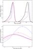 |
Fig. 3 Top panel: simulated light curves: the thick black curve represents the one at low energies; the others show three different examples of higher energy data. The left-hand curves show the case when leading sides are delayed with respect to the low energy, but the trailing sides are the same in two cases and slightly different in the third one. In the right-hand curves, different shifts between the pulse maxima and decays are introduced. Bottom panel: the cross-correlation functions for the simulated light curves normalised to the values of zero lag. Colours are the same as the corresponding simulated data. |
A precise definition of this effect is not simple. To illustrate this, we consider some simulated, one low-energy, and three high-energy, light curves as shown in Fig. 3 (top panel). In the three examples on the left-hand side, high-energy curves have the leading sides delayed with respect to the low-energy curves, but the trailing sides are the same in two cases and slightly different in the third one. In the other two examples (on the right-hand side of the bottom panel in Fig. 3), we considered different lags between the pulse maxima and the following decays. It is apparent that delays are not constant during the bursts and reach the highest values at the transition between the SLT and the pulse. Taking into account the conventional definition of a signal width, we can consider the pulse height at half of the maximum and define the HXDs as the separation between these values at different energies. Thus, the horizontal segments plotted between the couples of pulses in Fig. 3 (upper panel) give an estimate of these delays, which are equal to 1.75, 4.0, and 5.25 s for the left three bursts and to 5.75 and 10.25 s for the other two, while peak shifts are 2.5 and 5.0 s. We must also distinguish between the delays occurring in the rising and decaying portions of the burst, hereafter indicated as HXD1 and HXD2, because they can be different. The evaluation of lags between signals in two simultaneous time series is generally performed by means of their cross-correlation function (CCF). This method is not sensitive to the variables we are working with and other algorithms must be applied. This is clearly shown in the CCF plots of the above simulated data in the bottom panel of Fig. 3: CCF maxima for the first set of three burst data sets have very low values in the range 0.5–1.5 s, which are much smaller than the separation between pulses. In the other two examples, CCF maxima are clearly evident, but their lags are 3.5 and 6.0 s, slightly higher than the corresponding peak shifts, but even much lower than the separations at half peak heights. These examples show that the CCF method does not always provide a proper evaluation of HXD: it is much more sensitive to phase lags at the fundamental frequency, where it is the highest power, but it does not measure well lags at higher harmonics, which are important when the pulse width is changing, as in our case. In addition to CCF, we have therefore considered other methods which are more appropriate for a self-consistent description of the burst inherent complexity.
4. Limit cycle mapping in the CR–E plane
To study the evolution of recurrent signals, it is useful to analyse the trajectories described in a suitable parameter space defined by two or more variables. It is therefore necessary to have at least two simultaneous time series of independent quantities. For dynamical systems, one could consider, for example, the time derivative of the original data series as an independent variable. In our case, however, because of rather large fluctuations of the signal, the calculated derivatives present frequent sign changes and the resulting trajectories are highly confused. We thus preferred to use a dynamic space, having the count rate and the mean photon energy as coordinates (hereafter CR-E plane). Hardness ratios (HR) could be used equivalently instead of the mean energy, and we verified that the two variables are strongly correlated, as expected. We recall that the dominant emission component in the MECS range is the multi-temperature disk (see Paper II); the mean photon energy can be related to the temperature Tin at the inner boundary of the disk, while the count rate can be related to the integrated photon emission rate from the disk (see Sect. 5.3). For this reason we preferred to use the mean energy instead of HR. We note that these variables are statistically independent, at variance with the plots of two hardness ratios (see, e.g. Vilhu & Nevalainen 1998; Belloni et al. 2000), where there is an interdependence between the two variables due to the use of count rates in a common energy band. This parameter space cannot be considered equivalent to the phase space used in the study of dynamical systems because the curves can intersect and can also be superimposed: different brightness states can correspond to the same mean photon energy. A more complete description of the physical state of the disk, in fact, would require more than two variables.
For a better understanding of the evolution of a system in the CR-E plane, one must consider that trajectories described by sources exhibiting variations with a one-to-one correspondence between the mean photon energy and the count rate are portions of a curve that becomes a straight segment when they are exactly proportional. The occurrence of loops implies that there is a time shift between the two variables, and the direction of the motion along the loop depends on the sign of the lag between the mean energy and the count rate. This approach can be considered an evolution of the method that was originally proposed by Milne (1934) for studying stellar variability, and some of the considerations developed in this paper can be applied in the present analysis.
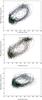 |
Fig. 4 Trajectories for the data of the A8b (top panel), E5 (central panel), and F7 (bottom panel) time series in the CR-E plane. Dotted lines connect consecutive data points, the green dots are the mean values in the set of angular sectors along the loop, and thick lines are their best fit ellipses, computed as described in the text; crosses mark the centroids of the trajectories. |
The CR-E trajectories for the A8b, E5, and F7 series are reported in the top, central, and bottom panel of Fig. 4, respectively: the loop structure is clearly apparent in all the panels, but with some interesting differences. First, we note that all loops are in a counterclockwise direction, which in our case corresponds to a lag of the mean energy series as expected from the occurrence of HXD, either in the SLT or in the decay of the pulse, which is a stable characteristic of the ρ class. Data points are not uniformly distributed along the cycle: their density is generally much higher in the low-energy – low-count rate part of the diagram. This region corresponds to the SLT segment, while the pulse, which completes the right-upper part of the loop, evolves on a shorter time-scale and has therefore a smaller number of points. In the CR-E map of the E5 series, there is another high density region in the high-energy and high count rate part, corresponding to the high multiplicity structure of the pulse, and trajectories describe smaller secondary loops. Our CR-E plots are strongly similar to that presented in Fig. 14 of Janiuk & Czerny (2005), where they considered the two regions with a high density of points, which are also present in our maps. However, in that work the trajectories were not considered as a tool for the HXD evaluation.
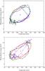 |
Fig. 5 Trajectories in the CR-E plane of two subsequent individual bursts of the A8b (top panel) and E5 (bottom panel) time series. Green filled circles and blue and red ellipses are the mean trajectories and the best fits as in Fig. 4; black lines connecting consecutive points track individual bursts, with the exception of the first “anomalous” burst in the bottom panel plotted as a violet dashed line. In the upper panel the thick black portions of the line connecting data points mark the sections used to measure the HXD1 (magenta) and HXD2 (orange). |
4.1. Mean trajectories: definition and main properties
As a first step, we evaluated the central point encircled by the CR-E plane trajectories. A direct evaluation of this point from a simple averaging of CR-E coordinates of all data points would produce a position that is close to the high-density region in the left-hand bottom side and not even encircled by several burst loops. We therefore adopted the following procedure: we assumed a preliminary guess for the point location and transformed the two variables by subtracting these approximate values and normalizing them by dividing the resulting values by the respective standard deviations. From this point, we then drew a set of angular beams covering the entire plane, with an amplitude chosen to have in each of them a minimum number of 50 points; we computed the mean of the radial distances of all points inside each bin and assigned this value to the central beam direction. All these points track a first mean trajectory, and their mean values were used to calculate a new central point (hereafter we refer this point as the centroid of the loop; it is independent of the normalization and can be easily translated to the original CR-E plane). This procedure was iterated until a convergence better than 0.5% and a stable mean trajectory was reached, The final trajectories are plotted as green dots in the panels of Figs. 4 and 5.
All the mean trajectories present a nearly elliptical shape and so, for each considered data series we computed the best-fitting ellipse; the results were found to track them quite well, with some minor deviations. According to Milne (1934), the elliptical shape can be understood on the basis of the hexagon Pascal’s theorem, assuming that there is a relation linking the mean energy with the count rate. Mean trajectories and best ellipses are also plotted for the CR-E maps in Fig. 4 and their centroids are marked by a cross. We note that the ellipses of the A8b and E5 series have similar orientation; the latter is only a bit more elongated along the major axis, whereas that of the F7 series is smaller and has a different orientation with the major axis nearly aligned with the CR axis. Moreover, from the plots of the A8b and E5 series, which correspond to the regular and irregular mode, respectively, we see that their centroids remained very stable (changes are smaller than 1%). This indicates that different types of bursts do not significantly depend on these parameters. We also note that, by our construction of the mean trajectories, they are rather regular curves without minor loops, and very different from those originated by peaks in bursts with high multiplicity. The information on structures related to the irregular mode does not appear in the mean trajectories, and their study must be based on the analysis of the trajectories of individual bursts (see Sect. 4.2).
4.2. Trajectories of individual bursts
As discussed above, the mean CR-E trajectories of all data series can be reasonably described by a regular curve like an ellipse. Ellipses described with a constant angular velocity would result as a combination of simple harmonic motions on both coordinates, and the orientation ellipse would depend on their phase difference. Time profiles of individual bursts, however, differ from a sinusoid on both variables and can exhibit several structures, depending on the SLT length and pulse multiplicity. Figure 5 shows some examples of trajectories for a couple of bursts extracted from the regular A8b series (upper panel) and the irregular E5 one (lower panel). In the former case, we see a burst following an elliptical loop rather well, while the second one, with two well-separated peaks (multiplicity 2), has a trajectory that crosses the ellipse and presents a second clockwise small loop in the upper region. As shown in Paper I, bursts in the regular series are characterised by a low mean multiplicity, which reaches 1.5 only in a few series. Consequently, the region surrounding the centroids of the ellipse does not appear to be crossed by many trajectories. Irregular series, like E5 (lower panel in Fig. 5), which have a typical mean multiplicity close to or higher than 2.5, tend to fill this central region. Moreover, they frequently present one or more secondary loops in the in the upper right-hand corner of their ellipses. The connections between this structure and the burst type are also discussed in Neilsen et al. (2012).
4.3. Evolution of trajectories with the mean count rate
The plots of Fig. 4 show that a change in the shape and orientation of the ellipse
occurred with the transition between interval II and III, when the the BL
count rate increased (see Papers I and II). This increase produced a shift of the
centroid of the loop (and its mean ellipse) with respect to those of the preceeding
series. A change in the ellipses’ orientation implies a variation of the phase difference
of the two variables. To make this effect clear, we investigated whether it can or cannot
be explained by a BL increase. To this aim, we modelled the burst
structure as the sum of a constant BL level plus a variable signal
representing the rate variation along the burst. We indicate with
Nk = NB + (NV)k
the total numbers of photons in each time bin k, where
NB and
NV are the photons in the BL
and variable component, respectively. Assuming that the mean energy of BL
photons remains stable at the value
⟨ EB ⟩, the mean photon energy will be
 (2)where
⟨ (EV)k ⟩ is
the mean energy of photons in the variable components in the kth bin. In
this simple model, we assumed that ⟨ EB ⟩
remained stable and equal to 4.25 keV during all the observation in agreement with the
disk/coronal temperature in the SLT-1 phase, as found in Paper II. For a
change of the BL count rate from
NB to
(2)where
⟨ (EV)k ⟩ is
the mean energy of photons in the variable components in the kth bin. In
this simple model, we assumed that ⟨ EB ⟩
remained stable and equal to 4.25 keV during all the observation in agreement with the
disk/coronal temperature in the SLT-1 phase, as found in Paper II. For a
change of the BL count rate from
NB to
 and consequently from
Nk to
and consequently from
Nk to
 , as observed in the II and III
time intervals, the mean photon energy would change to
, as observed in the II and III
time intervals, the mean photon energy would change to
 (3)We note that this
transformation is not a linear function in Δ, and therefore the ellipse will be changed in
another closed curve, but such a modification would be relevant only for high Δ values.
(3)We note that this
transformation is not a linear function in Δ, and therefore the ellipse will be changed in
another closed curve, but such a modification would be relevant only for high Δ values.
We applied this transformation to the A8b ellipse for Δ equal to the change of the mean count rates from A8b to F7 series and plotted the resulting curve together with the mean ellipses of the three series considered in Fig. 6: its position was similar to that of F7, but the orientation results changed slightly. We conclude that an increase of the BL count rate cannot explain the change in the orientation of the ellipse observed in the two regular modes in the time intervals I and III and that a phase difference between the two variables must also occur. Only for quite large Δ values is a clear change in the ellipse shape and orientation obtained, but in this case a large change of the highest count rates is also found in contrast with the observational results (see Fig. 4). This result also agrees with the conclusion derived from the spectral analysis from Paper II and Neilsen et al. (2012) that different modes require different disk temperatures and delays.
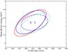 |
Fig. 6 Best-fit ellipses of the mean trajectories in the CR-E plane of the A8b (blue solid line), E5 (red solid line), and F7 (blue dashed line) series, showing the change of the shape, orientation, and location of the centre of the ellipse of the last data series with respect to the previous two. The green ellipse is computed from that of the A8b by increasing the count rate by the difference between the mean values with the F7 series and assuming that the mean energy of this component was unchanged, equal to 4.25 keV, as the typical BL value. |
5. HXD evaluation and results
We adopted two different approaches to evaluate the HXD. A first method, called the direct method, is based on the delay between the rising/decaying portions of individual bursts in the two series from their CR-E trajectories. The second method is the calculation of the cross-correlation function between the count rate and mean energy time series. This standard method was used as a benchmark for the results obtained with the limit cycle mapping.
5.1. Direct method results
To estimate the HXDs from the CR-E trajectories, we subtracted the corresponding values of the loops’ centroid from the count rate and mean energy data series and normalised the results by dividing the respective standard deviations. Then, we computed for every burst the time differences between the rising edges at their zero level to estimate HXD1 and between the corresponding decaying edges to estimate HXD2. In practice, HXD1 corresponds to the time necessary to cover the part of the trajectory marked by a thick magenta line in the upper panel of Fig. 5, and HXD2 corresponds to the time needed to cover the orange line. We representatively show a short segment of normalised count rate (black) and mean energy (red) curves used for the evaluation of HXD1 and HXD2 in Fig. 7. Both curves have a zero level corresponding to the centroid’s values of the loop. The time difference between the two curves at zero is HXD1 in the SLT and HXD2 in the FDT. These two examples clearly show the presence of a time lag between the maxima of the count rate and the mean energy series. This lag is due to the fact that the energy distribution of photons in the FDT has a temperature that, on average, is higher than the ones found in SLT and P-1; this effect lasts until the BL level is reached (see Paper II).
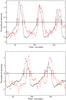 |
Fig. 7 Upper panel: a segment of the A8b series illustrating how HXDs are evaluated in single bursts. Black and red data are the count rate and mean energy series, respectively. The zero level corresponds to the values of the centroid of the ellipse in the CR − E plot. Long and short vertical bars mark the time intervals of HXD1 and HXD2, respectively. Lower panel: a segment of equal duration of the F7 series. We note that both HXDs are longer than in the A8b series. |
These values were then averaged over every time series; the resulting HXDs are given in Table 2 and plotted in Fig. 8 as red diamonds (HXD1) and open green squares (HXD2). In the regular series, HXD2 values are lower than the HXD1 ones, with an average difference of 0.6 s in the interval I that increases to 3 s in interval III. Only in three irregular series did we find HXD2 longer than HXD1. We note, however, that the estimate of HXD2 is more uncertain than HXD1 because of the irregularity of pulse decays due to the presence of several substructures, particularly in bursts with high multiplicity. When bursts exhibit such substructures, we assumed as HXD2 the smallest time difference.
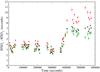 |
Fig. 8 Evolution of the HXDs, measured by means of the various methods, between the count rate and the mean energy data series during the entire time interval: results from the direct method are red diamonds (HXD1) and green open squares (HXD2). Black filled circle are the HXD values obtained from the cross-correlation method. The rather sharp increase from the interval II to III (360 000 to 400 000 s), after the irregular mode,corresponds to an increase in the mean count rate (see Paper I). |
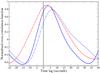 |
Fig. 9 Cross-correlation functions of the count rate and mean energy data of three series, divided for their number of time bins: A8b (blue solid line), E5 (red solid line) and F7 (blue dashed line). We note a time lag varying from about 2.5 s to more than 6 s. |
5.2. Cross-correlation results
To compare our estimates of the HXD with the results reported in the literature, we also computed the cross-correlation function (CCF) between the count rate and the mean energy for all the time series considered. The CCF functions of the three sample series are plotted in Fig. 9: all show a clear time lag of the mean energy series with respect to the count rate. The position of the first maximum is considered as an estimate of the mean shift between the two time series giving the best matching between them, so we cannot obtain information on HXD1 and HXD2 separately. We used a polynomial best fit to evaluate the position of CCF maxima, and the resulting values are given in Table 1 and plotted in Fig. 8. The CCF results are lower than HXD2 or between the two HXD values obtained by means of the direct method.
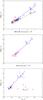 |
Fig. 10 Upper panel: correlation between the HXD1, evaluated using the direct method, with the third power of the mean count rate of the BL (in units of 106). Blue circles correspond to the interval I series, blue triangles to the interval III series; red filled squares correspond to the series in interval II. The solid thick violet line indicates the linear best fit. Black circles and the thin black line are data points for the CCF estimates of HXD and their best fit. Central panel: correlation between the mean HXDs with the mean count rate in the PDS band (units of 105). Symbols are the same as in the upper panel. Lower panel: correlation between the mean HXD1 with the recurrence time of bursts as evaluated in Paper I. The solid thick line is the linear best fit of blue points only. Black circled points mark the irregular data series. |
5.3. Evolution of the HXD
The time evolution of the HXD measures is remarkably similar to that of the mean count rate and a very interesting behaviour emerges: the HXD remained practically stable within the rather narrow range [3–4] s during the interval I, when GRS 1915+105 was in the regular mode. A small decrease occurred in the interval II, during the irregular mode, which was followed by a rather sharp increase between 360 ks and 400 ks to a mean lag value around 7 s, when the source turned again to the regular mode interval III. As shown in Fig. 8, this evolution of HXD in the course of the observation is remarkably similar to those of other quantities that characterise the ρ class (see Paper I), particularly the BL count rate (see Fig. 15 in Paper I). To show this, we use a double-log plot of HXD vs. count rate. A power-law fit with an exponent close to three provides a good description of this apparent trend. This result is shown in the upper panel of Fig. 10, where we plotted the values of the HXD1, against the third power of the count rate (in units of 106 counts3). The resulting linear correlation coefficient is equal to 0.982. We note that this exponent value depends on the method used to estimate the HXD; in fact, by repeating the same analysis with the values derived from the CCF method, we obtained a power law index closer to 2.5.
In the upper panel of Fig. 10, these values are also plotted together with the linear best fit, corresponding to a linear correlation coefficient equal to 0.974. According to the timing analysis of Paper I, this result implies that HXD1 is also related to the mean count rate of PDS (15–100 keV) and to the recurrence time of the bursts. The former correlation is shown in the central panel of Fig. 10, where HXD1 is plotted against the third power of the PDS count rate (the linear correlation coefficient is 0.973), while the one with the recurrence time is shown in the lower panel of the same figure. In this case, however, it is important to distinguish regular series from the irregular ones: in the latter mode, in fact, it is very difficult to evaluate a reliable value of Trec. Fourier periodograms of irregular series are generally of M type (Paper I) with several prominent peaks, and the central value of the period range in which they are present was used in the plot. These series, which occurred mainly in interval II, appear to be characterised by rather short HXDs. For the series of intervals I and III, which are mostly regular, we again obtained a very high linear correlation coefficient equal to 0.958; the corresponding best fit is plotted in Fig. 10.
Loops in the CR-E plane can also be depicted in terms of corresponding spectral parameters (see also Neilsen et al. 2011, 2012). In Paper II we evaluated temperatures and fluxes for the multi-temperature disk and a surrounding hot corona component in five burst segments; their plots are given in Fig. 11. The general structure of the loops in the CR-E plane of Figs. 4 and 11 can be easily recognized in the disk plot.
Using the results of the spectral analysis presented in Paper II, we constructed the
light curves for the multi-temperature disk and for the corona emission. They were
obtained from the detected rates according to the following formula
 (4)where
Rcomp is the rate relative to each spectral component at the
time t, Rtotal the detected rate,
fcomp and ftotal are the
component and total fluxes in the considered energy range. These factors depend on the
source spectrum and change along the five burst segments that we identified in each
series. Short portions of the light curves for the multi-temperature disk and the corona
for the three series A8b, E5, and F7, previously considered in this paper, are shown in
the three panels of Fig. 12. In each panel we
plotted the computed count rates in three energy ranges [1.7–3.4], [3.4–6.8] and
[6.9–10.2] keV. We note that the pulse appears only in the disk component
curve (black curve) and that the high-energy peaks lag behind the ones in the soft range
with a behaviour coherent with the HXDs detected in our analysis. The corona emission is
rather stable, particularly at energies above ~7 keV, while in the lowest range it is
strongly anti-correlated with the disk component.
(4)where
Rcomp is the rate relative to each spectral component at the
time t, Rtotal the detected rate,
fcomp and ftotal are the
component and total fluxes in the considered energy range. These factors depend on the
source spectrum and change along the five burst segments that we identified in each
series. Short portions of the light curves for the multi-temperature disk and the corona
for the three series A8b, E5, and F7, previously considered in this paper, are shown in
the three panels of Fig. 12. In each panel we
plotted the computed count rates in three energy ranges [1.7–3.4], [3.4–6.8] and
[6.9–10.2] keV. We note that the pulse appears only in the disk component
curve (black curve) and that the high-energy peaks lag behind the ones in the soft range
with a behaviour coherent with the HXDs detected in our analysis. The corona emission is
rather stable, particularly at energies above ~7 keV, while in the lowest range it is
strongly anti-correlated with the disk component.
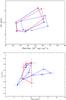 |
Fig. 11 Upper panel: evolution of spectral parameters of the disk component (see Paper I, Table 2) in the five segments of the bursts in the three intervals: I (solid blue line); II (solid red line); III (dashed blue line). Lower panel: evolution of spectral parameters of the coronal component (see Paper I, Table 2) in the same five segments of the bursts as in the upper panel. |
6. Discussion
We have shown that trajectories in the CR-E plane provide a useful tool for investigating the complex behaviour of binary X-ray sources, particularly when they exhibit quasi-periodic variations as GRS 1915+105 does in the ρ class. An interesting parameter for the physical modelling is the delay of the X-ray emission in the hard X-ray range with respect to the soft band. We developed a method based on the study of these trajectories to measure the HXD values observed in the burst sequence. Our results offer a wider perspective on the HXD phenomenon in GRS 1915+105 . In particular, we have shown that in the ρ class the hard time lag can vary significantly, from ~3 s up to ~10 s, in tight correlation with the BL count rate and likely proportional to its third power. This general evolution, despite some minor systematic deviations, is consistent with the results obtained by means of the CCF between the count rate and the mean energy data series, which is sensitive to the phase lags between the two signals.
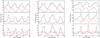 |
Fig. 12 Short segments 200 s long of the count rates of the light curves for the multi-temperature disk (black) and the corona (red) emission components in the three energy ranges [1.7–3.4] (top), [3.4–6.8] (centre), and [6.9–10.2] keV (bottom) for the three series A8b (left panel), E5 (central panel), F7 (right panel). Rates relative to the corona were multiplied by 8 in the energy range [1.7–3.4] keV and by 2 in the other ranges to superimpose the light curves on the disk ones. |
Neilsen et al. (2012) reported in some RXTE observations a relation between HXD and burst multiplicity that is not evident from the BeppoSAX data examined in this work. This follows from the different definitions and methods used to evaluate the HXD, because we focused our analysis mainly on HXD1, which occurs in the transition between the SLT and the P − 1 and is not expected to be related to the peak multiplicity. Particularly interesting is the finding that the HXD1 is highly correlated with some important source parameters, such as the baseline level of the stable component onto which bursts are superposed and the mean PDS count rate (see Table 2).
This result can imply that the development of the limit cycle, which is typical of ρ bursts, is physically related to the state of the disk and that it can depend on some relevant quantities, such as the accretion mass rate and the local temperature value.
A phenomenon similar to HXD, as considered by us, is also observed at much lower frequencies in other disk accretion systems such as dwarf novae. In the outbursts of some nova-like sources, it was noticed that the rise of high-frequency radiation follows that of the optical with a variable delay, ranging from minutes to days (UV: e.g. Hassall et al. 1983, 1985; Cannizzo et al. 1986; soft X: van der Woerd et al. 1986), while the decline in the two bands occurs almost simultaneously.
6.1. Physical origin of the HXD
The geometry and physical characteristics of the corona of GRS 1915+105 are still debated. One possibility is to set the corona at the base of a jet (Nobili 2003), anchoring a source of variability in the accretion disk (like a flaring magnetic episode or a density wave) and adjusting in a suitable way the distance from the jet and its opening angle. However, such scenarios seems unlikely for the ρ class bacause it has been associated with unstable jet formation and generally weak radio emission (Klein-Wolt et al. 2002). A more plausible scenario could be connected to a hot, geometrically thick compact corona and a truncated accretion disk, whose inner radius loops between a maximum and a minimum (possibly associated with the last stable orbit radius) value. These models have been successful in reproducing the general light curve shapes typical of the ρ class (Honma et al. 1991; Szuszkiewicz & Miller 1998; Taam et al. 1997; Janiuk et al. 2000) and rely on the classical thermal instability model of Lightman & Eardley (1974) as the agent of the cyclic behaviour. Another scenario, which is more physically motivated, is based on a geometrically thin and cold accretion disk (but with a variable and opportune prescription for the viscosity) and a corona above it (Nayakshin et al. 2000).
A first attempt to derive from this model an explanation for the hard lag phenomenon was provided by Janiuk & Czerny (2005), which presented a simple interaction model between disk and corona that provided, at least qualitatively, the observed time-scales. The model assumed a mass exchange between disk and corona, but the coronal thermodynamic equilibrium was simply set by the virial temperature (Compton processes are thus neglected). Besides providing the observed time-scale of the lag (~1 s), the model produced anti-correlated disk and coronal light curves, and predicted luminosity variations of the corona within a factor of two between the minimum and maximum fluxes. These predictions are in good agreement with what we observationally found. The new observational facts that add now up are the correlation between the baseline count rates and the hard time lag and the wide spread in values of the observed lags.
Finally, always within the instability model, it is possible to interpret the hard lag as a typical thermal time-scale of the region of the disk, which experiences the instability producing the limit cycle behaviour. While the viscous disk time-scale sets the recurrence time of the outbursts (Belloni et al. 1997), it is expected that the thermodynamic time-scale should be at least a factor 10 less, of the same order of the rising outburst time-scales (Nayakshin et al. 2000). As shown in Fig. 12, the most variable component in the MECS energy range is always associated with the thermal disk emission. We argue therefore that such hard lags could be mostly due to the thermal adjustment of the rising/decaying temperature within the inner parts of the disk, which are probably due to mass-accretion variations propagating in the disk.
The regularity and the rather stable HXD, which are often observed in the ρ class bursts, suggest that it can be described by a set of differential equations, likely including one or more non-linear terms that combine the evolution of luminosity and temperature. The parameters in these equations, in turn, could vary on time-scales different from that of the bursts, e.g. the mass accretion rate; they could be responsible for systematic changes exhibited by the source and also produce changes of variability class. A first attempt to construct a mathematical model for the ρ class appears very promising and, if confirmed,will be the subject of a forthcoming paper.
The discovery of another source, IGR J17091-3624, which also shows the heartbeat phenomenon typical of the ρ class of GRS 1915+105, opened the possibility to place much stronger constraints on the physical interpretation of such complex behaviours. This new source has shown so far several of the variability classes originally discovered in GRS 1915+105, albeit on faster time-scales and seemingly at lower accretion luminosities. Further and more detailed comparative studies of the two sources are needed to improve our understanding of the Eddington/radiation pressure instability as a function of disk (corona) viscosity, accretion rate, optical depth, radiative efficiency, and mass transfer prescriptions.
Online material
Observation runs of the BeppoSAX pointing of GRS 1915+105 in October 2000 used in the HXD analysis.
Acknowledgments
The authors thank the personnel of ASI Science Data Center, particularly M. Capalbi, for help in retrieving BeppoSAX archive data and the anonymous referee for his/her useful comments of the paper. A.D. and T.M. thank Prof. A. A. Zdziarski for his useful discussion on the analysis. This work has been partially supported by research funds of the Sapienza Università di Roma.
References
- Altamirano, D., Belloni, T., Linares, M., et al. 2011, ApJ, 742, L17 [NASA ADS] [CrossRef] [Google Scholar]
- Belloni, T., Mendez, M., King, A. R., van der Klis, M., & van Paradijs, J. 1997, ApJ, 488, L109 [NASA ADS] [CrossRef] [Google Scholar]
- Belloni, T., Klein-Wolt, M., Méndez, M., van der Klis, M., & van Paradijs, J. 2000, A&A, 355, 271 [NASA ADS] [Google Scholar]
- Boella, G., Chiappetti, L., Conti, G., et al. 1997, A&AS, 122, 327 [NASA ADS] [CrossRef] [EDP Sciences] [Google Scholar]
- Cannizzo, J. K., Wheeler, J. C., & Polidan, R. S. 1986, ApJ, 301, 634 [NASA ADS] [CrossRef] [Google Scholar]
- Cassatella, P., Uttley, P., Wilms, J., & Poutanen, J. 2012, MNRAS, 422, 2407 [NASA ADS] [CrossRef] [Google Scholar]
- Cui, W. 1999, ApJ, 524, L59 [NASA ADS] [CrossRef] [Google Scholar]
- Hassall, B. J. M., Pringle, J. E., Schwarzenberg-Czerny, A., et al. 1983, MNRAS, 203, 865 [NASA ADS] [Google Scholar]
- Hassall, B. J. M., Pringle, J. E., & Verbunt, F. 1985, MNRAS, 216, 353 [NASA ADS] [Google Scholar]
- Honma, F., Kato, S., Matsumoto, R., & Abramowicz, M. A. 1991, PASJ, 43, 261 [NASA ADS] [Google Scholar]
- Janiuk, A., & Czerny, B. 2005, MNRAS, 356, 205 [NASA ADS] [CrossRef] [Google Scholar]
- Janiuk, A., Czerny, B., & Siemiginowska, A. 2000, ApJ, 542, L33 [NASA ADS] [CrossRef] [Google Scholar]
- Klein-Wolt, M., Fender, R. P., Pooley, G. G., et al. 2002, MNRAS, 331, 745 [NASA ADS] [CrossRef] [Google Scholar]
- Lightman, A. P., & Eardley, D. M. 1974, ApJ, 187, L1 [NASA ADS] [CrossRef] [Google Scholar]
- Massaro, E., Ventura, G., Massa, F., et al. 2010, A&A, 513, A21 [NASA ADS] [CrossRef] [EDP Sciences] [Google Scholar]
- Milne, E. A. 1934, MNRAS, 94, 418 [NASA ADS] [Google Scholar]
- Mineo, T., Massaro, E., D’Ai, A., et al. 2012, A&A, 537, A18 [NASA ADS] [CrossRef] [EDP Sciences] [Google Scholar]
- Muno, M. P., Remillard, R. A., Morgan, E. H., et al. 2001, ApJ, 556, 515 [NASA ADS] [CrossRef] [Google Scholar]
- Nayakshin, S., Rappaport, S., & Melia, F. 2000, ApJ, 535, 798 [NASA ADS] [CrossRef] [Google Scholar]
- Neilsen, J., Remillard, R. A., & Lee, J. C. 2011, ApJ, 737, 69 [NASA ADS] [CrossRef] [Google Scholar]
- Neilsen, J., Remillard, R. A., & Lee, J. C. 2012, ApJ, 750, 71 [NASA ADS] [CrossRef] [Google Scholar]
- Nobili, L. 2003, ApJ, 582, 954 [NASA ADS] [CrossRef] [Google Scholar]
- Paul, B., Agrawal, P. C., Rao, A. R., et al. 1998, ApJ, 492, L63 [NASA ADS] [CrossRef] [Google Scholar]
- Reig, P., Belloni, T., van der Klis, M., et al. 2000, ApJ, 541, 883 [NASA ADS] [CrossRef] [Google Scholar]
- Szuszkiewicz, E., & Miller, J. C. 1998, MNRAS, 298, 888 [NASA ADS] [CrossRef] [Google Scholar]
- Taam, R. E., Chen, X., & Swank, J. H. 1997, ApJ, 485, L83 [NASA ADS] [CrossRef] [Google Scholar]
- Uttley, P., Wilkinson, T., Cassatella, P., et al. 2011, MNRAS, 414, L60 [NASA ADS] [Google Scholar]
- van der Woerd, H., Heise, J., & Bateson, F. 1986, A&A, 156, 252 [NASA ADS] [Google Scholar]
- Vilhu, O., & Nevalainen, J. 1998, ApJ, 508, L85 [NASA ADS] [CrossRef] [Google Scholar]
All Tables
Observation runs of the BeppoSAX pointing of GRS 1915+105 in October 2000 used in the HXD analysis.
All Figures
|
Fig. 1 Two 300-s long segments of the count rate (upper panels) and mean photon energy (lower panels) curves of the MECS [1.7–10] keV data series A8b (left), E5 (centre), and F7 (right) after a running average smoothing over five bins. The bin size of all series is 1 s. |
| In the text | |
|
Fig. 2 Portions of MECS light curves in the energy ranges [1.3−3.4] keV, green curve, and [6.8–10.2] keV, blue curve. From top to bottom, examples from time interval I (time series A8b), time interval II (E5), and time interval III (F7). The time bin is 1 s. |
| In the text | |
|
Fig. 3 Top panel: simulated light curves: the thick black curve represents the one at low energies; the others show three different examples of higher energy data. The left-hand curves show the case when leading sides are delayed with respect to the low energy, but the trailing sides are the same in two cases and slightly different in the third one. In the right-hand curves, different shifts between the pulse maxima and decays are introduced. Bottom panel: the cross-correlation functions for the simulated light curves normalised to the values of zero lag. Colours are the same as the corresponding simulated data. |
| In the text | |
|
Fig. 4 Trajectories for the data of the A8b (top panel), E5 (central panel), and F7 (bottom panel) time series in the CR-E plane. Dotted lines connect consecutive data points, the green dots are the mean values in the set of angular sectors along the loop, and thick lines are their best fit ellipses, computed as described in the text; crosses mark the centroids of the trajectories. |
| In the text | |
|
Fig. 5 Trajectories in the CR-E plane of two subsequent individual bursts of the A8b (top panel) and E5 (bottom panel) time series. Green filled circles and blue and red ellipses are the mean trajectories and the best fits as in Fig. 4; black lines connecting consecutive points track individual bursts, with the exception of the first “anomalous” burst in the bottom panel plotted as a violet dashed line. In the upper panel the thick black portions of the line connecting data points mark the sections used to measure the HXD1 (magenta) and HXD2 (orange). |
| In the text | |
|
Fig. 6 Best-fit ellipses of the mean trajectories in the CR-E plane of the A8b (blue solid line), E5 (red solid line), and F7 (blue dashed line) series, showing the change of the shape, orientation, and location of the centre of the ellipse of the last data series with respect to the previous two. The green ellipse is computed from that of the A8b by increasing the count rate by the difference between the mean values with the F7 series and assuming that the mean energy of this component was unchanged, equal to 4.25 keV, as the typical BL value. |
| In the text | |
|
Fig. 7 Upper panel: a segment of the A8b series illustrating how HXDs are evaluated in single bursts. Black and red data are the count rate and mean energy series, respectively. The zero level corresponds to the values of the centroid of the ellipse in the CR − E plot. Long and short vertical bars mark the time intervals of HXD1 and HXD2, respectively. Lower panel: a segment of equal duration of the F7 series. We note that both HXDs are longer than in the A8b series. |
| In the text | |
|
Fig. 8 Evolution of the HXDs, measured by means of the various methods, between the count rate and the mean energy data series during the entire time interval: results from the direct method are red diamonds (HXD1) and green open squares (HXD2). Black filled circle are the HXD values obtained from the cross-correlation method. The rather sharp increase from the interval II to III (360 000 to 400 000 s), after the irregular mode,corresponds to an increase in the mean count rate (see Paper I). |
| In the text | |
|
Fig. 9 Cross-correlation functions of the count rate and mean energy data of three series, divided for their number of time bins: A8b (blue solid line), E5 (red solid line) and F7 (blue dashed line). We note a time lag varying from about 2.5 s to more than 6 s. |
| In the text | |
|
Fig. 10 Upper panel: correlation between the HXD1, evaluated using the direct method, with the third power of the mean count rate of the BL (in units of 106). Blue circles correspond to the interval I series, blue triangles to the interval III series; red filled squares correspond to the series in interval II. The solid thick violet line indicates the linear best fit. Black circles and the thin black line are data points for the CCF estimates of HXD and their best fit. Central panel: correlation between the mean HXDs with the mean count rate in the PDS band (units of 105). Symbols are the same as in the upper panel. Lower panel: correlation between the mean HXD1 with the recurrence time of bursts as evaluated in Paper I. The solid thick line is the linear best fit of blue points only. Black circled points mark the irregular data series. |
| In the text | |
|
Fig. 11 Upper panel: evolution of spectral parameters of the disk component (see Paper I, Table 2) in the five segments of the bursts in the three intervals: I (solid blue line); II (solid red line); III (dashed blue line). Lower panel: evolution of spectral parameters of the coronal component (see Paper I, Table 2) in the same five segments of the bursts as in the upper panel. |
| In the text | |
|
Fig. 12 Short segments 200 s long of the count rates of the light curves for the multi-temperature disk (black) and the corona (red) emission components in the three energy ranges [1.7–3.4] (top), [3.4–6.8] (centre), and [6.9–10.2] keV (bottom) for the three series A8b (left panel), E5 (central panel), F7 (right panel). Rates relative to the corona were multiplied by 8 in the energy range [1.7–3.4] keV and by 2 in the other ranges to superimpose the light curves on the disk ones. |
| In the text | |
Current usage metrics show cumulative count of Article Views (full-text article views including HTML views, PDF and ePub downloads, according to the available data) and Abstracts Views on Vision4Press platform.
Data correspond to usage on the plateform after 2015. The current usage metrics is available 48-96 hours after online publication and is updated daily on week days.
Initial download of the metrics may take a while.