| Issue |
A&A
Volume 555, July 2013
|
|
|---|---|---|
| Article Number | A52 | |
| Number of page(s) | 22 | |
| Section | Astronomical instrumentation | |
| DOI | https://doi.org/10.1051/0004-6361/201219605 | |
| Published online | 01 July 2013 | |
INTEGRAL/SPI data segmentation to retrieve source intensity variations⋆
1 Université de Toulouse, UPS – OMP, IRAP, 31028 Toulouse Cedex 04, France
e-mail: This email address is being protected from spambots. You need JavaScript enabled to view it.
2 CNRS, IRAP, 9 Av. colonel Roche, BP 44346, 31028 Toulouse Cedex 4, France
3 Université de Toulouse, INPT – ENSEEIHT – IRIT, 31071 Toulouse, Cedex 7, France
4 CNRS-IRIT, 31071 Toulouse Cedex 7, France
5 Lawrence Berkeley National Laboratory, Berkeley CA 94720, USA
Received: 15 May 2012
Accepted: 22 April 2013
Abstract
Context. The INTEGRAL/SPI, X/γ-ray spectrometer (20 keV–8 MeV) is an instrument for which recovering source intensity variations is not straightforward and can constitute a difficulty for data analysis. In most cases, determining the source intensity changes between exposures is largely based on a priori information.
Aims. We propose techniques that help to overcome the difficulty related to source intensity variations, which make this step more rational. In addition, the constructed “synthetic” light curves should permit us to obtain a sky model that describes the data better and optimizes the source signal-to-noise ratios.
Methods. For this purpose, the time intensity variation of each source was modeled as a combination of piecewise segments of time during which a given source exhibits a constant intensity. To optimize the signal-to-noise ratios, the number of segments was minimized. We present a first method that takes advantage of previous time series that can be obtained from another instrument on-board the INTEGRAL observatory. A data segmentation algorithm was then used to synthesize the time series into segments. The second method no longer needs external light curves, but solely SPI raw data. For this, we developed a specific algorithm that involves the SPI transfer function.
Results. The time segmentation algorithms that were developed solve a difficulty inherent to the SPI instrument, which is the intensity variations of sources between exposures, and it allows us to obtain more information about the sources’ behavior.
Key words: methods: data analysis / methods: numerical / techniques: miscellaneous / techniques: imaging spectroscopy / methods: statistical / gamma rays: general
Based on observations with INTEGRAL, an ESA project with instruments and science data centre funded by ESA member states (especially the PI countries: Denmark, France, Germany, Italy, Spain, and Switzerland), Czech Republic and Poland with participation of Russia and the USA.
© ESO, 2013
1. Introduction
The SPI X/γ-ray spectrometer, on-board the INTEGRAL observatory is dedicated to the analysis of both point-sources and diffuse emission (Vedrenne et al. 2003). The sky imaging is indirect and relies on a coded-mask aperture associated to a specific observation strategy that is based on a dithering procedure. Dithering is needed since a single exposure does not always provide enough information or data to reconstruct the sky region viewed through the ~30° field-of-view (FoV), which may contain hundreds of sources for the most crowded regions. It consists of small shifts in the pointing direction between exposures, the grouping of which allows us to increase the amount of available information on a given sky target through a growing set of “non-redundant” data. The standard data analysis consists of adjusting a model of the sky convolved with the instrument transfer function plus instrumental background to the data.
However, source intensities vary between exposures. Thus, a reliable modeling of source variability, at least of the most intense ones, is needed to accurately model the data and intensity measurement of the sources. In addition, ignoring these intensity variations can prevent the detection of the weakest sources.
Ideally, the system of equations that connects the data to the sky model (unknowns) should be solved for intensities as well as for the variability timescales of sources and background. We propose methods based on data segmentation to fulfill these requirements as best as possible and we report in detail on the improved description and treatment of source variability during the data reduction process.
2. Functioning of SPI: necessity of modeling the intensity variations of sources
2.1. Instrument
SPI is a spectrometer provided with an imaging system sensitive to both point-sources and extended source/diffuse emission. The instrumental characteristics and performance are described in Vedrenne et al. (2003) and Roques et al. (2003). Data are collected between 20 keV and 8 MeV using 19 high-purity Ge detectors illuminated by the sky through a coded mask. The resulting FoV is ~30°. The instrument can locate intense sources with an accuracy of a few arc minutes (Dubath et al. 2005).
2.2. SPI imaging specifics and necessity of dithering
A single exposure provides only 19 data values (one per Ge detector), which is not enough to correctly sample the sky image. Indeed, dividing the sky into ~2° pixels (the instrumental angular resolution) yields about 225 unknowns for a 30° FoV (i.e., (30°/2°)2). Hence, reconstructing the complete sky image enclosed in the FoV is not possible from a single exposure because the related system of equations is undetermined. From these 19 data values, and the parameters describing the instrumental background we can, at best, determine the intensity of only a few sources. This is sufficient for sparsely populated sky regions and for obtaining a related coarse image (the intensities of the few pixels corresponding to the source positions). However, some of the observed sky regions are crowded (the Galactic center region, for example, contains hundreds of sources) and obtaining more data is mandatory for determining all parameters of the sky model. The dithering technique (Sect. 2.3) allows to obtain this larger set of data through multiple exposures.
2.3. Dithering
By introducing multiple exposures of the same field of the sky that are shifted by an offset that is small compared to the FoV size, the number of data related to this sky region is increased. In the dithering strategy used for INTEGRAL, the spacecraft continuously follows a dithering pattern throughout an observation (Jensen et al. 2003). In general, the exposure direction varies around the pointed target by steps of 2° within a five-by-five square or a seven-point hexagonal pattern. An exposure lasts between 30 min and 1 h.
Through grouping of exposures related to a given sky region, the dithering technique allows one to increase the number of “non-redundant” data points1 without significantly increasing the size of the FoV that is spanned by these exposures. This provides enough data to recover the source intensity by solving the related system of equations. The source intensity variations within an exposure do not constitute a problem with the coded mask imaging system. The difficulty comes from the intensity variations between exposures. Hence, in our case, sources are variable on various timescales, ranging from an hour (roughly the duration of an exposure) to years. This information should be included in the system of equations to be solved.
2.4. Handling source intensity variation
We chose to model the intensity variation of a source as a succession of piecewise constant segments of time. In each of the segments (also called “time bins”), the intensity of the source is supposed to be stable. The higher energy bands (E ≳ 100 keV) contain a few emitting/detectable sources. Their intensities are rather stable with time according to the statistics and only a few piecewise constant segments of time or “time bins” are needed to model source intensity variations.
At lower energies (E ≲ 100 keV), the source intensity varies more rapidly. When inappropriate timescales are used for the sources contained in the resulting large FoV (>30°) and for the background, the model does not fit the data satisfactorily (the chi-squares of the corresponding least-squares problem (Appendix A) can be relatively high). Moreover, allowing all sources to vary on the timescale of an exposure is an inappropriate strategy because, for crowded regions of the sky the problems to be solved are again undetermined in most cases. Generally, to estimate the source variability timescale, a crude and straightforward technique consists of testing several mean timescale values until the reduced chi-square of the associated least-squares problem is about 1 or does not decrease anymore. Unfortunately, this method is rapidly limited. Including variability in the system of equations always increases the number of unknowns that need to be determined (Appendix A) since the intensity in each segment of time (“time bins”) is to be determined. Using too many “time bins” will increase the solution variance and does not necessarily produce the best solution. Similarly, it is better to limit the number of “time bins” to the strict necessary minimum to set up a well-conditioned system of equations.
When one manually defines the “time bins”, one might soon be overwhelmed by the many timescales to be tested and the number of sources. It is difficult to simultaneously search for the variability of all sources contained in the instrument FoV and to test the various combinations of “time bins” (not necessarily the same length or duration, location in time). As a consequence, constructing light curves turns out to be rather subjective and tedious, and relies most of the time on some a priori knowledge. To make this step more rational, we propose methods based on a partition of the data into segments, to model source intensity variations between exposures.
3. Material
The objective is to find the “time bins” or segment sizes and locations corresponding to some data. This is related to the partition of an interval of time into segments. We propose two methods. The first one, called “image space”, relies on some already available light curves (or equivalently on a time series)2. In our application the time series come mainly from INTEGRAL/IBIS and from Swift/BAT (Barthelmy et al. 2005). The purpose is to simplify an original light curve to maximize the source signal-to-noise ratio (S/N), hence to reduce the number of “time bins” through minimizing of the number of time segments3. These “time bins” are used to set up the SPI system of equations. This partitioning is made for all sources in the FoV. This algorithm is not completely controlled by SPI data, but at least it allows one to obtain a reasonable agreement (quantified by the chi-square value) between the data and the sky model.
The second method, called “data space”, starts from the SPI data and uses the instrument transfer function. In contrast to the “image-space” method where the segmentation is made for a single source only, the “data-space” method performs the time interval partitioning simultaneously for all sources in the FoV and is used to separate their individual contributions to the data. While this is more complex, the great advantage is that it is based solely on SPI data (Sect. 5).
Index of mathematical symbols.
4. Theory and calculation
4.1. The “image-space” algorithm – partition of a time series
The partition of an interval into segments is closely related to the topic of change points, which is widely discussed in the literature. There is a variety of efficient ways to analyze a time series if the parameters associated with each segment are independent (Fearnhead 2006; Hutter 2007, and references therein). Scargle (1998) proposed an algorithm for best data partitioning within an interval based on Bayesian statistics. Applications to astronomical time series (BATSE bursts characterization) can be found in Scargle (1998).
4.2. Problem formulation
A list of notations used throughout this paper is given in Table 1. We consider the time series x ≡ x1:L = (x1,...,xL), comprising L sequential elements, following the model  (1)where xi are the measured data and ϵi their measurement errors. The data are assumed to be ordered in time, although they may be spaced irregularly, meaning that each xi is associated with a time ti and contained in a time interval T = (t1,...,tL). f(ti) is the model to be determined. We chose to model the time series as a combination of piecewise constant segments of time or blocks. This set of non-overlapping blocks that add up to form the whole interval forms a partition of the interval T. Hence there are, m change points τ1:m = (τ1,...,τm), which define m + 1 segments, such that the function f(t) is constant between two successive change points,
 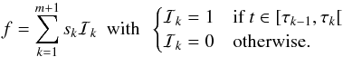 (2)Here τ0 = min(T) and τm + 1 = max(T) or, equivalently, in point number units, τ0 = 1 and τm + 1 = L + 1 (τ0 < τ1 < ... < τm + 1). Since these data are always corrupted by observational errors, the aim is to distinguish statistically significant variations through the unavoidable random noise fluctuations. Hence, the problem is fitting a function through a noisy one-dimensional series, where the function f to be recovered is assumed to be a piecewise constant function of unknown segment numbers and locations (see Appendix A).
4.3. Algorithm
Yao (1984) and Jackson et al. (2005) proposed a dynamic programing algorithm to explore these partitions. The algorithm described in Jackson et al. (2005) finds the exact global optimum for any block additive fitness function (additive independent segments) and determines the number and location of the necessary segments. For L data points, there are 2L − 1 possible partitions. In short, these authors proposed a search method that aims at minimizing the following function (see also Killick et al. 2012): ![Mathematical equation: \begin{equation} \min_{{\tau}} \left\{\sum_{i=1}^{m+1}{\left[\mathcal{C}(x_{(\tau_{i-1}+1):\tau_i}) + \beta \right]}\right\}, \label{eqn:objf} \end{equation}](/articles/aa/full_html/2013/07/aa19605-12/aa19605-12-eq71.png) (3)where
(3)where  represents some cost function. The ith segment contains the data block x(τi − 1 + 1):τi = (xτi − 1 + 1,...,xτi) (in point number units), and the cost function or effective fitness for this data block is
  ). The negative log-likelihood, for example the chi-square, is a commonly used cost function in the change point literature, but other cost functions can be used instead (e.g. Killick et al. 2012, and references therein). β is a penalty to prevent overfitting. Jackson et al. (2005, but see also Killick et al. 2012 proposed a convenient recursive expression to build the partition in L passes,
  (4)This enables calculating the global best segmentation using best segmentations on subsets of the data. Once the best segmentation for the data subset x1:τ∗ has been identified, it is used to infer the best segmentation for data x1:τ∗ + 1.
At each step of the recursion, the best segmentation up to τ∗ is stored; for that, the position of the last change point τ∗ is recorded in a vector (Jackson et al. 2005). By backtracking this vector, the positions of all change points that constitute the best segmentation at a given time or iteration number can be recovered. Figure 1 shows a flowchart of the algorithm. Our implementation is essentially the same as that of Jackson et al. (2005), but see also Killick et al. (2012). The best partition of the data is found in O(L2) evaluations of the cost function.
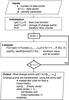 |
Fig. 1 Flowchart of the “image-space” algorithm (pseudo-code in Appendix F.1). The vector last gives the starting point of individual segments of the best partition in the following way; let τm=last(L), τm − 1=last(τm − 1) and so on. The last segment contains cells (data points) τm,τm + 1,...,n, the next-to-last contains cells τm − 1,τm − 1 + 1,...,τm − 1, and so on. |
5. “Data-space” algorithm
The SPI data contain the variable signals of several sources. The contribution of each of the sources to the data through a transfer function is to be retrieved. As in Sect. 4.1 and for each of the sources, the number and positions of segments are the parameters to be estimated, but this time, the estimates are interdependent because of the nature of the instrument coding. While many algorithms exist to analyze models where the parameters associated with each segment are independent of those linked to the other segments, there are only a few approaches, not of general applicability, where the parameters are dependent from one segment to another (Punskaya et al. 2002; Fearnhead & Liu 2011, and references therein). However, our problem involves a transfer function, which requires a specific treatment.
5.1. Contribution of the sources to the data
The elements related to source J are denoted with the upper subscript (J). The variable signal of the source numbered J is represented by nseg(J) ( = m(J) + 1) piecewise constant segments (“time bins”) delimited by 0 ≤ m(J) ≤ np − 1 change points (Sect. 4.2). The response H0(1:M,J) , which corresponds to a constant source intensity, is a vector of length M ( ). This vector is expanded into a submatrix with nseg(J) orthogonal columns. The signal can be written (see also Eq. (2))
 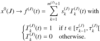 The corresponding predicted contribution to the data, at time t (in units of exposure number), is
 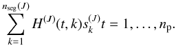 The submatrices H(J)(t,k) of dimension nd(t) × nseg(J) are derived from the response vector H0(1:M,J) as follows:
 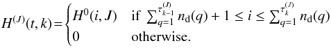 The response associated with the N0 sources is obtained by grouping subarrays H(J) of all sources,
 ![Mathematical equation: \begin{equation} H \equiv \left[H^{(1)},\cdots,H^{(N^0)} \right]. \label{eqn:gather}\\ \end{equation}](/articles/aa/full_html/2013/07/aa19605-12/aa19605-12-eq97.png) (5)Matrix H has size M × N with
(5)Matrix H has size M × N with  . Therefore, the predicted contribution of the N0 variable sources to the data is
 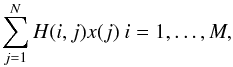 where
where 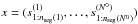 is the flux in the N “time bins” (see also Appendix A).
5.2. Algorithm
The search path or the number of possible partitions for N0 sources and the np exposures is (2np − 1)N0. An exhaustive search is not feasible for our application. In addition, computing the cost function for a particular partition implicitly involves solving a system of equations (computing the cost function), which renders the search even more inefficient. We essentially make a simplification or approximation that reduces the computation time, allows significant optimizations, and hence makes the problem tractable.
Instead of searching for the exact change points, we can settle for reliable segments and hence derive an algorithm that aims at significantly reducing the search path. Rather than exploring the space for all sources simultaneously, we explore the reduced space associated to a single source at a time. The algorithm closely follows the pattern of Eq. (4). It is an iterative construction of time segments that processes the sources sequentially and independently. In practice, the best set of change points using the data recorded up to time t − 1 is stored. The nd(t) new data points obtained at time t are added to the dataset. The procedure starts for the best change points recorded so far. For a given source, an additional change point is added at the various possible positions. Its best position is recorded along with the best new cost function. The operation is repeated for all sources. The best change point (and cost function value) of all sources is kept (location and source number) and added to the growing set of change points. This procedure is repeated several times, for instance Niter (≤N0 subiteration) times, until no more change points are detected or until the cost function cannot be improved any further. Then, another iteration at t + 1 can start. Figure 2 schematically shows the resulting procedure.
This experimental approach is exact when the columns of the transfer matrix are orthogonal. Although there is no mathematical proof that this holds for a matrix that does not have this property, it is efficient on SPI transfer function and data (Sect. 6.3).
 |
Fig. 2 Flowchart of the “data-space” algorithm (pseudo-code in Appendix F.2). The cost function calculation, here the shaded box, is detailed in Fig. 3. |
5.3. Cost function calculation
The computation of the cost function, used to adjust the data to the model, is detailed in Appendix B. The derived expression involves the minimization of the chi-square function. Indeed, the cost function must be computed many times, each time that a new partition is tested. This is by far the most time-consuming part of the algorithm. Fortunately, these calculations can be optimized.
At iteration n, for a subiteration, we have to solve about n × N0 systems of equations to compute the cost functions corresponding to the different change-point positions. Instead of solving all these systems, it is possible to solve only a few of them and/or reduce the number of arithmetic operations by relying on the structure of the matrices4.
The matrix H of size M × N using the change points obtained at iteration n − 1 is the starting point. To search for the best partition for source J, we have to replace only the submatrix H(J) by its updated version H∗ (J). The corresponding transfer matrix H∗ (of dimension M × N∗) can be written (Eq. (5)) as ![Mathematical equation: \begin{eqnarray*} {\bf H}^*(1:M,1:N^*) \equiv \left[{\bf H}^{(1)},\cdots,{\bf H}^{(J-1)}, {\bf H}^{*(J)}, {\bf H}^{(J+1)},\cdots, {\bf H}^{(N^0)}\right]. \end{eqnarray*}](/articles/aa/full_html/2013/07/aa19605-12/aa19605-12-eq114.png) The dimension of the submatrix H∗ (J) corresponding to the new data partition is
The dimension of the submatrix H∗ (J) corresponding to the new data partition is  . Here
  is the resulting number of segments for source J. It varies from 1, which corresponds to a single segment for the source J, to the
  , where
  is the highest number of segments obtained so far for source J for iteration up to n − 1. In most cases, only the few last columns of the matrix H∗ (J) are not identical to those of H(J), since the very first columns tend to be frozen (Sect. 5.4). If
  is the number of consecutive identical columns, then
 ![Mathematical equation: \begin{eqnarray*} {\bf H}^{*(J)} \equiv \left[{\bf H}^{(J)}(1:M,1:n_{\rm seg}^{\rm keep} ), H_{\rm add}(1:M,1:N_{\rm add}) \right]. \end{eqnarray*}](/articles/aa/full_html/2013/07/aa19605-12/aa19605-12-eq121.png) Here Hadd is the modified part of H(J). Let
Here Hadd is the modified part of H(J). Let  and
and  . Then, the columns, from
  to kmax(J) are deleted in the matrix H and Nadd columns are added at position to
  . Therefore, it is not necessary to compute the full matrix H∗ from scratch each time a new change point is tested (position and source number), but simply to update some columns of the matrix H. This construction of the transfer function significantly saves on run time and provides clues to further optimization.
However, in our application, we solve a least-squares system, and hence the matrix A = HTH (A∗ = H∗ TH∗) is to be implicitly inverted. We use an expression based on the Sherman-Morrison-Woodbury formula and the matrix partition lemma (E) to obtain A∗ from A after subtracting Nsub and added Nadd columns to H (Appendix E). With this optimization, we need only one matrix decomposition (A = LtL where L is a lower triangular matrix) of a symmetric sparse matrix5A of order N per iteration and solve the system (Ax = HTy) (store factors and solution). Then, for each tested change-point position tested, only one system of equations is to be solved (using the matrix decomposition stored previously), other operations are relatively inexpensive. To compute the cost function, it can be necessary for our application, depending on the expression of the cost function, to compute a determinant. However, in our application, only the ratio of the determinant of the created matrix (A∗) of rank N∗ = N + Nadd − Nsub to matrix A of rank N matters. This ratio is very stable because it involves only matrices of small rank. In addition, as a cross-product of the update of A, it is inexpensive to compute.
5.4. “Limited memory” version
The number of possible partitions, and hence possible change-point positions, increases with the number of exposures (Sect. 5.2). This makes the problem difficult to solve in terms of computing time for data sets containing a large number of exposures. The positions of the change points are not necessarily fixed until the last iteration. In the worst case, there can be no common change points (hence segments) between two successive iterations. In practice, it turns out that they become more or less frozen once a few successive change points have been located. Then, for each source, instead of exploring the n possible positions of the change point, we consider only the data accumulated between iteration n0 > 1 and n (The “full” algorithm starts at n0 = 1). This defines a smaller exploration window size, which further reduces the number of cost function evaluations (in the shaded box of Fig. 3, the loop on change-point positions starts at i = n0 > 1). The number of change-point positions to test is nearly stable as a function of the number of accumulated exposures. Section 6.3.4) compares the “limited memory” and “full” version.
 |
Fig. 3 Flowchart of the calculation of the cost function for the “data-space” algorithm. |
5.5. Parallelization
The algorithm sequentially divides each source interval into segments. Hence, it is straightforward to parallelize the code and process several sources simultaneously. To do so, the “source loop” (in the shaded box of Fig. 3, the loop on J) is parallelized using Open-MP. Matrix operations are performed in sequential mode, although a parallel implementation is also possible. Experiments on parallelization are presented in Sect. 6.3.3.
6. Results
The sky model for each dataset consists of sources plus the instrumental background, whose intensity variations are to be determined. The background is also the dominant contributor to the observed detector counts or data. Its spatial structure on the detector plane (relative count rates of the detectors) is assumed to be known thanks to “empty-field” observations, but its intensity is variable (Appendix A). By default, its intensity variability timescale is fixed to ~6 h, which was shown to be relevant for SPI (Bouchet et al. 2010). Its intensity variation can also be computed, as for a source, with the “data-space” algorithm.
Owing to observational constraints (solar panel orientation toward the Sun, etc.), a given source is “visible” only every ~6 months and is observed only during specific dedicated exposures (Fig. 4). For these reasons, it is more convenient to present the “light curves” as a function of the exposure number, so the abscissa does not actually reflect the time directly.
The fluxes obtained with SPI and IBIS in each defined “time bin”, are also compared whenever possible. However, IBIS light curves are provided by a “quick-look analysis” and are intended to give an approximate measurement of the source intensity. These time series, used as external data input to the “image-space” method, are not fully converted into units that are independent of the instrument (such as photons cm2 s-1) and can even be affected by the specific characteristics of the instrument.
6.1. Datasets/training data
The various datasets used in this paper are shorter subsets related to a given sky region of a larger database that consists of ~39 000 exposures covering six years of observations of the entire sky (Bouchet et al. 2011). An SPI dataset, related to a particular source, consists of all exposures whose angular distance, between the telescope pointing axis and the source of interest direction (central source), is less than 15°. This procedure gathers the maximum number of exposures containing the signal from the source of interest, but at the same time the datasets span a ~30° radius FoV sky region containing numerous sources.
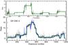 |
Fig. 4 GX 339-4 intensity variations. The 26–40 keV IBIS time series (gray), which contains 1183 data points (one measurement per exposure), is segmented into 17 constant segments or “time bins” (green). The |
Concerning the energy bandwidth of the datasets, the transfer function is computed for the same mean energy. However, because of the spectral evolution of the source with time, this approximation introduces some inaccuracies that increase with the energy bandwidth. At first glance, it is preferable to use a narrow energy band, but at the same time, the S/N of the sources are lower (since the error bars on the fluxes are large enough, we detected virtually no variation in intensity). In other words, for a narrower energy band, the reduced chi-square between the data and the model of the sky is lower, but at the same time, the source intensity variations are less marked. Finally, as a compromise for our demonstration purpose, we used the 25–50 keV and 27–36 keV energy bands.
6.2. “Image-space” method
6.2.1. Application framework
We rely on auxiliary information, such as available light curves, to define the “time bins” for SPI. These light curves come from the IBIS “quick-look analysis”6, more precisely, its first detector layer ISGRI (Ubertini et al. 2003). The light curves of the known sources are not all available, but usually the strongest ones are, if not always exactly in the requested energy bands, but this is sufficient to define some reliable “time bins”.
The “image-space” method consists of two separate steps. The first does not necessarily involve the SPI instrument, while the second one involves the SPI only.
6.2.2. “Time bins”: segmentation of an existing time series
The basic process to set up the “time bin” characteristics (position and length) is the time series segmentation. The raw time series is the light curve linked to a given source, which comes from the “quick-look analysis” of IBIS data. Below 100 keV, IBIS is more sensitive than SPI. However, it depends on the source position relative to the instrument pointing axis, the number of sources in the FoV, but also on the source’s spectral shape. The measured S/N of the two instruments for strong sources is around ~2 and increased to ~3 for crowded sky regions. To have roughly similar S/N per sources between IBIS and SPI, especially in crowded sky regions, random Gaussian statistical fluctuations are added to raw time series to obtain statistical error bars on IBIS light curves increased roughly by a factor 3 below 100 keV. This forms the time series used. This ad hoc procedure is also retrospectively coherent with the number of segments obtained with the “data-space” method (Sect. 6.5). Above 150 keV SPI is more sensitive, but at these energies many sources can be considered to be stable in intensity because their detection significance is low (fluxes have large error bars), hence we do not expect as many “time bins”.
In principle, the model of the time series, hence the number of segments, can be adjusted to the data with the desired chi-square value by varying the penalty parameter β of Eq. (3). Intuitively, one readily sees that a too high value will underfit, while a too low value will overfit the data. To be conservative, we adjusted this parameter to obtain a reduced chi-square ( ) of 1; the segmentation algorithm is fast enough to test several values of β to achieve this objective.
We proceeded as follows: if a single segment (constant flux) gives above 1, the time series was segmented. Many expressions of the cost function can be used; expressions C.3 and C.5 described in Appendix C give similar results. Finally, we chose the most simple one (C.3), which is the chi-square function.
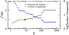 |
Fig. 5 GX 339-4 time series segmentation. Variation of the |
Figures 4 and 5 show the application to the GX 339-4 source, whose intensity variation is characterized by a short rise time followed by an exponential decay on a timescale of about one month. The IBIS time series for the 26–40 keV band contains 1183 exposures. The is 1.0006 for 1166 degrees of freedom (d.o.f.), the number of “time bins” is 17 for a penalty parameter value of 8.99 (if the IBIS raw time series is directly segmented7, the number of segments is 46 instead of 17).
6.2.3. Application to SPI
We applied the “image-space” algorithm to the common IBIS/SPI 27–36 keV datasets related to the GX 339-4, 4U 1700-377, and GX 1+4 sources, which contain 1183, 4112, and 4246 exposures. The persistent source 4U 1700-377 is variable on hour timescales, while GX 1+4 is variable on a timescale from days to about 1–2 months. In the sky model are 120, 142, and 140 sources included for the GX 339-4, 4U 1700-377, and GX 1+4 datasets.
For 4U 1700-377, the reduced chi-square ( ) between the predicted and measured data is 6.15; assuming that all sources have constant intensity, this value is clearly not acceptable. Each available IBIS individual light curve was segmented as indicated in Sect. 6.2.2 to define the “time bins”. A total number of 4005 “time bins” was obtained to describe the dataset, and the resulting 4U 1700-377 was partitioned into 2245 segments. The SPI-related system of equations (Appendix A) was then solved using these segments. The is 1.28 for 68 455 d.o.f., which is a clear improvement compared with the value of 6.15 obtained when all sources are assumed to remain constant over time. It is also possible to directly use the “time bins” defined with the IBIS light curves without scaling the sensitivities of the two instruments (Sect. 6.2.2), in which case the reaches 1.13. For strong and highly variable sources such as 4U 1700-377, one can fix the variation timescale to the exposure duration (~1 h). All these results are summarized in Table 2.
For all three datasets, the source 4U 1700-377 was assumed to vary on the exposure timescale. Assuming that all other sources are constant in intensity yields a final of 2.46, 1.81, and 2.01 for the GX 339-4, GX 1+4, and 4U 1700-377 datasets.
The segmentation of the available IBIS time series permits one to obtain better “time bins” and the improves to values below 1.2 (Table 2). The resulting GX 339-4 and GX 1+4 light curves were partitioned into 17 and 122 segments (Table 2). Figure 6 shows the intensity variations of these two sources, obtained from SPI data.
The correlation of the fluxes in the “time bins” of the two instruments is purely indicative since IBIS time series are obtained from a “quick-look analysis”. However, the fluxes are well correlated (Fig. 8). The linear correlation coefficients are 0.995, 0.941, and 0.816, for GX 339-4, 4U 1700-377, and GX 1+4.
To illustrate the decreasing number of “time bins” with increasing energies, we used the GRS 1915+105 dataset. There are 1185 common IBIS and SPI exposures for this source in our database. For each energy band, the procedure is the same as before, but with 66 sources contained in the FoV. The number of “time bins” after segmentation of the IBIS time series in the 27–36, 49–66, 90–121 and 163–220 keV bands, is 174, 50, 8, and 1 and the (d.o.f.), after solving the SPI related system of equations, is 1.20 (20 257), 1.05(20 545), 1.02(20 562), and 1.01(20 616). Figure 7 shows the resulting intensity variations.
“Image-space” method final chi-square.
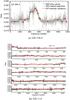 |
Fig. 6 Intensity variations of GX 339-4 and GX 1+4 in the 27–36 keV band as a function of the exposure number. The SPI segments are plotted in red and the IBIS raw light curves (26–40 keV) are drawn in gray. The segmented IBIS time series (scaled S/N) is shown in green. The count rate normalization between IBIS and SPI is arbitrary. |
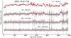 |
Fig. 7 “Image-space” method applied to GRS 1915+105. The intensity variations as a function of the exposure number are shown in the 27–36, 49–66, 90–121 and 163–220 keV band as indicated in the figure. The different bands are translated on-to the y-axis (the intensities are in arbitrary units). The SPI segments are plotted in red and the IBIS time series (scaled S/N) are drawn in gray (26–40, 51–63, 105–150, and 150–250 keV). The number of “time bins” deduced from the time series segmentation are 174, 50, 8, and 1. The global normalization factor in each energy band between the fluxes of the two instruments is arbitrary. |
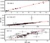 |
Fig. 8 IBIS/SPI flux correlation in 17, 2245, and 122 “time bins” for GX 339-4, 4U 1700-377, and GX 1+4. The red line is a straight-line fitting (with errors in both directions) with a chi-square of 25 (15 d.o.f.), 3961 (2243 d.o.f.), and 321 (120 d.o.f.). |
6.3. “Data-space” method
6.3.1. Application framework
As examples, we built datasets related to the sources V0332+53, Cyg X-1, GRS 1915+105, GX 339-4, and IGR J17464-3213 as described in Sect. 6.2. The characteristics of these datasets are indicated in Table 3.
Characteristics of the datasets.
6.3.2. Cost function, penalty parameter, and chi-square
The penalty parameter value determines the final chi-square value between the data and the sky model, but its choice is more problematic than with the “image-space” algorithm. Figure 9 illustrates the influence of parameter β on the final number of segments and the value for several datasets of Table 3. Because of the very schematic representation of the data, it is not always possible to reach a value of 1 for all these datasets, but this value can be approached; if necessary, the width of the energy bands can be reduced (Sect. 6.1) to obtain a lower value. Two expressions of the cost function are used using different assumptions (Appendix C), but there is no strong justification for preferring one expression over the other.
The simplest cost function expression C.8 is essentially the chi-square. The value of the penalty parameter β prescribed by the Bayesian information criterion is β0 ~ log (M), M being the number of data points (Appendix D). A penalty parameter value lower than this prescription is required to reach a value closer to 1. These lower values of β produce a greater number of “time bins”, which has the effect of reducing the chi-square at the expense of the reliability of the solution. However, the value β0 remains a reliable guess value of the penalty parameter and gives a number of “time bins” similar to what is expected from the direct segmentation of the light curves (Sect. 6.5).
Expression C.9 of the cost function has an additional term with respect to the expression C.8, which acts as a penalty parameter and further limits the increase of the number of “time bins”. The minimum cost function value is reached for penalty parameters β below one tenth of β0. A value β = 0 can be used since it gives the minimum chi-square or at least a value close to the lowest one. The value is then comparable to the value obtained with expression C.8 and the Bayesian information criterion prescription for the value of β.
Figure 9 shows the evolution of the and total number of segments to describe the intensity variations of the central source as a function of the penalty parameter β for several datasets and configurations of the “data-space” algorithm. The C.8 expression of the cost function permits one to reach a lower value of the chi-square compared to C.9. Tables 6 and 7 summarize the results obtained with the “data-space” method. We quite arbitrarily chose to use the expression C.9 as the baseline cost function with penalty parameter β = 0.
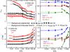 |
Fig. 9 (Bottom) Reduced chi-square ( |
6.3.3. Parallelization
Table 4 shows experimental results for two datasets (V0332+53 and GX 339-4 (Table 3). A system with 64 (2.62 GHz) cores was used. The run time was measured in the “source loop” (Sect. 5.5). Using 16 threads instead of 1 speeds up the computation by a factor ~3 for the V0332+53 dataset and by a factor ~4 for the GX 339-4 with the “limited memory” code. The gain is the same for the V0332+53 dataset with the “full” code, but the average time to perform a loop is about seven times higher than the “limited memory” code.
Gain in time achieved by “source loop” parallelization of the “data-space” algorithm.
6.3.4. “Limited memory” and “full” version
The “limited memory” version (Sect. 5.4) is parameterized such that at iteration n, it starts the change-points position exploration at exposure n0 = min(n − 30 exposures, n − 2 change points backward), individually for each source.
For the GX 339-4 dataset, the average time spent in a single “source loop” by the “full” version increases with the iteration number (number of exposures processed) while it is comparable per iteration number with the “limited memory” version. Table 5 reports the gain in time achieved with the “limited memory” version compared with the full “data-space” algorithm. Finally, the “limited memory” version is almost ~15 times faster than the “full” version on the GX 339-4 dataset.
Mean time spent in the “source loop” by the “full” and “limited memory” versions of the ’data-space’ algorithm.
Table 7 compares the results of the “limited memory” and “full” version for the V0332+53 and GX 339-4 and the GRS 1915+105 and Cyg X-1 datasets. The number of segments found by the “limited” version is in general slightly higher than the number found by the “full” version of the code; however, this effect is also due to the particular parametrization used for the “limited” version. The results remain quite similar in terms of number of segments and reached , showing that the “limited memory” version is a good alternative to the full “data-space” algorithm, especially for the gain in computation time. The gain in time of the “limited” (with the above parametrization) over the “full” version reaches a factor ~30 when the background timescale is fixed (not to be segmented).
6.3.5. Background segmentation
It is no longer necessary to fix the variation timescale of instrumental background to about six hours. The “data-space” algorithm models the change in intensity of the background similarly to the other sources of the sky model (Table 7). If we let the algorithm determine the background intensity variation, it is modeled with a fewer number of segments than when the background variation is fixed for a quantitatively comparable chi-square. This is because of a better localization of the change points. The other parameters, such as the number and locations of the source “time bins”, stay essentially the same.
6.3.6. Application
The “limited memory” version, where the intensity variations of both sources and background are computed, was used as the default algorithm. For the dataset relative to V0332+53, this consisted of a of 1.06 for 6595 d.o.f. and a total of 97 “time bins”. The resulting V0332+53 intensity evolution is displayed in Fig. 10 as a function of the exposure number (nine segments).
Next, we processed the highly variable source Cyg X-1. The dataset is 1.44 for 40 068 d.o.f. and a total of 676 “time bins”. The number of segments needed to describe Cyg X-1 is 280. The relatively high value of the chi-square may be due to the strong intensity and hence to the high S/N of the source. However, the systematic errors due to the finite precision of the transfer function start to be important for this strong source, which may be in part responsible for the high chi-square value.
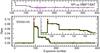 |
Fig. 10 ‘’Data-space” method applied to V0332+53. The source intensity variations (25–50 keV) were modeled by nine segments (red) and were compared with the IBIS time series (26–51 keV, gray). The green curve corresponds to the IBIS flux averaged on SPI-obtained segments. The insert is a zoom between exposure number 81 and 179. (Top) SPI intensity variations model (black) compared with Swift/BAT time series (24–50 keV, purple line). The scale between the different instruments is arbitrary and was chosen such that their measured total fluxes are equal. It should be noted that the Swift/BAT and IBIS data are not necessarily recorded at the same time as the SPI data, nor exactly in the same energy band. |
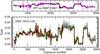 |
Fig. 11 Same caption as Fig. 10, but for GRS 1915+105 in the 27–36 keV band. The intensity linear correlation coefficients are 0.98 between IBIS (26–40 keV) and SPI, and 0.97 between Swift/BAT (24–35 keV) and SPI. |
For the dataset related to GRS 1915+105, a moderately strong and variable source, the is 1.24 for 51 573 d.o.f. and a total of 440 “time bins”. GRS 1915+105 intensity variation is displayed in Fig. 11 and consists of 106 segments.
The flux linear correlation factors between SPI and IBIS (“quick-look analysis”) fluxes measured in the same “time bins” are 0.991, 0.948, and 0.983 for V0332+53, Cyg X-1, and GRS 1915+105. The linear correlations with Swift/BAT are 0.993, 0.934, and 0.973. The flux correlation for Cyg X-1 and GRS 1915+105 are shown in Fig. 12. In addition, the average flux in a given segment is not necessarily based on the same duration of the observation. The number of usable SPI and IBIS exposures contained in the same segment is not always the same and there are not always simultaneous observations available of the same sky region by Swift/BAT and INTEGRAL. Despite these limitations, the fluxes measured by these instruments are quantitatively well correlated.
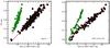 |
Fig. 12 Black denotes the SPI-IBIS correlation and green the SPI-Swift/BAT flux correlation in the “time bins” defined using the “data-space” method. The best SPI-IBIS and SPI-Swift/BAT linear regression are shown in red and purple. Left shows Cyg X-1 and right GRS 1915+105. |
Lower values of the chi-square than those indicated in Table 7 can be obtained by reducing the width of the energy band (Sect. 6.1) or by using a lower penalty parameter (Sect. 6.3.2) if the cost function is given by expression C.8.
“Limited-memory” “data-space” algorithm results.
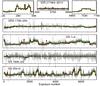 |
Fig. 13 Intensity evolutions (red) of IGR J17464-3213, GRS 1758-258, GX 1+4, GS 1826-24, and GX 354-0 in the 27–36 keV band. The IGR J17464-3213 dataset is divided in-to three subsets (dashed vertical lines show the limits) during the computation. The IBIS time series (30–40 keV) is shown in gray and the averaged fluxes in SPI “time bins” are plotted in green, as in Fig. 10. The distance of GRS 1758-258, GX 1+4, GS 1826-24, and GX 354-0 to IGR J17464-3213 are 7.3, 8.1, 12.7, and 3.4°. |
The IGR J17464-3213 dataset corresponds to the central, crowded, region of the Galaxy. The sky model consists of 132 sources and the background timescale was fixed to about six hours. The dataset is relatively large (7147 exposures) and was artificially split into three subsets to reduce the computation time. The characteristics of these three subsets are displayed in Table 6. The intensity variations of the central source, IGR 17464-3213, was modeled with 29 segments. We also extracted the intensity evolutions of GRS 1758-258, GX 1+4, GS 1826-24, and GX 354-0 which are derived simultaneously (Fig. 13). There are a few spikes in the GX 1+4 intensity variations, which are not investigated here in more detail. The comparison of the source intensity variations obtained with the IBIS instrument (the light curves are assembled from a “quick-look analysis”, the intensities are computed/averaged in the temporal segments found by the “data-space” method) gives linear correlation coefficients of 0.995, 0.800, 0.786, 0.845, and 0.901 for IGR J17464-3213, GRS 1758-258, GX 1+4, GS 1826-24, and GX 354-0. The comparison with Swift/BAT gives 0.996, 0.912, 0.909. 1.00, and 0.968 for the same sources.
“Data-space” algorithm comparison.
6.4. Comparison of the “image-space” and “data-space” methods
The comparison was made on the SPI and IBIS common 1183 exposures related to the GX 339-4 dataset. The “image-space” algorithm used the IBIS (26–40 keV) light curve as external input to define SPI “time bins”. It achieved a of 1.19 (18 880 d.o.f.) and a total of 1990 “time bins” and used 17 segments to describe the intensity evolution of GX 339-4 (Sect. 6.2). The “data-space” algorithm displays a similar of 1.20 and used 15 segments. Both light curves are compared in Fig. 14. If the background intensity is forced to vary on a timescale of about six hours, the number of segments is 13, if the source 4U 1700-377 is forced to vary exposure-by-exposure, the number of segments is 13 as well. The SPI curves are more difficult to compare quantitatively because the total number of segments and the are not the same with the two methods (Sect. 6.5). Nevertheless, we compared them indirectly with the IBIS binned ones. This demonstrates the effectiveness of the “data-space” algorithm.
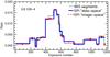 |
Fig. 14 Comparison of GX 339-4 (27–36 keV) intensity variations obtained with the “image-space” and the “data-space” algorithms. The common SPI/IBIS database contains 1183 exposures. The “image space” method describes GX 339-4 intensity variations with 17 segments (red) for a |
6.5. Studying a particular source: Obtaining its light curve on the exposure timescale
The data related to a given source also contain the contribution of the many other sources in the FoV. To study this particular source, one must take into account the influence of the other sources and distinguish the different contributions to the data. This means knowing the model of the intensity variations of all other sources. At the same time, the number of unknowns to be determined in the related system of equations must be minimum to achieve a high S/N for the source of interest. The intensity variation of all sources of the FoV is not generally known a priori and constitutes a difficulty. The “image-space” or “data-space” methods are designed to solve this difficulty.
The first step consists of processing data using methods that allow one to construct synthetic intensity variations of the sources; then one determines these variations by constructing “time bins” while minimizing their number. The intensity variations of all sources are fixed, excepted those of the source of interest, which can be therefore studied in more detail.
As an example, the procedure was applied to the GX 339-4 light curve study exposure-by-exposure. Figure 15 shows the light curve obtained with SPI, compared with its segmented version. The light curve is segmented into 15 segments, this number is comparable to the number found using IBIS time series of 17 segments, which also confirms the idea that it is useful to adjust the SPI and IBIS sensitivity.
Next, both GX 339-4 source and background were forced to vary exposure-by-exposure. The S/N of this GX 339-4 light curve is degraded compared with the case where the background varies on a timescale of about six hours or is segmented. The resulting light curve is segmented in-to only six segments. This illustrates the importance of having a minimum number of parameters to model the sky and the background.
 |
Fig. 15 “Data-space” algorithm has modeled the temporal evolution of GX 339-4 in the 27–36 keV band with 15 constant segments (blue). The light curve (in gray) of GX 339-4 was obtained by directly processing SPI data (after fixing the temporal evolution of the other sources). It contains 1183 data points (one measurement per exposure) The red curve is the segmentation of the gray curve into 15 segments with the “image space” algorithm. (*) If the background is forced to vary exposure-by-exposure, the GX 339-4 light curve is segmented only into six segments (dashed-green). |
7. Discussion and summary
7.1. Discussion
We proposed two methods for modeling the intensity variations of sky sources and instrumental background. The first one, called “image space”, is relatively easy to implement and benefits from the IBIS instrument on-board INTEGRAL, which simultaneously observes the same region of the sky as SPI. Hence in this case, the main weakness of this method is that it requires information from other instruments and then depends both on the characteristics of these instruments (FoV, sensitivity, etc.) and on the level of processing performed on these available external data.
The second method, called “data space” (Sect. 5), is based solely on SPI data and does not depend on external data. With this algorithm, the background intensity variations can be computed (6.3.5). The dependence across segments through the transfer function greatly increases the complexity of the algorithm, which is very computer-intensive and hence time-consuming. We have made some simplifications to be able to handle the problem and optimizations that in most cases accelerate the computations, in particular the way the matrices are updated during the change-point position search. More or alternative optimizations are possible, although we did not explore them in this paper; for example a (sparse) Cholesky update/down-date may be used at each iteration to avoid the decomposition of matrix H at each iteration. Similarly, an alternative to the procedure used here could be solving the orthogonal-least-squares problem through QR rank update. Because of the approximations we made, the best segmentation (in the mathematical sense) is probably not achieved, but at least we obtained a reliable one, which is sufficient to improve the sky model.
The final value of the chi-square is not really directly controlled for the “image-space” method. For the “data space”, the value achieved depends mainly on the value of the penalty parameter. We empirically derived some initial guess values. The determination of the penalty parameter, even if a good guess of its initial value is possible, and the cost function formulation are difficulties of the “data-space” method, which need more investigation.
In addition, the “data-space” method is more suitable for exploring the interdependence of the source contributions to the data. It takes into account the co-variance of the parameters during the data reduction process. In contrast, the “image-space” method uses only the variance since the light curves are already the product of another analysis and the covariance information related to the sources in the FoV is lost.
We chose to use a very simple representation of the source intensity variations by using piecewise constant functions. With this modeling of the time series, the individual segments are disjoint. For the “data-space” method and for a given (single) source, the columns of the corresponding submatrix are orthogonal. With a more complex light curve model, this property no longer holds. However, it is possible to derive a formulation where the intensity variations are continuous, e.g., using piecewise polynomials (the quadratic functions have been studied by Fearnhead & Liu (2011).
7.2. Summary
With only 19 pixels, the SPI detector does not provide enough data to correctly construct and sample the sky image viewed through the aperture. The dithering technique solves this critical imaging problem by accumulating “non-redundant” data on a given sky region, but at the same time it raises important questions of data reduction and image/data combination because of the variability of the sources.
We proposed two algorithms that model the intensity variation of sources in the form of combinations of piecewise segments of time during which a given source exhibits a constant intensity. For our purposes, these algorithms can help to solve a specific difficulty of the SPI data processing, which is to take into account the variability of sources during observations and consequently optimize the signal-to-noise ratio of the sources. A first algorithm uses existing time series to build segments
of time during which a given source exhibits a constant intensity. This auxiliary information is incorporated into the SPI system of equations to be solved. A second algorithm determines these segments directly using SPI data and constructs some “synthetic” light curves of the sources contained in the FoV. It separates the contribution to the data of each of the sources through the transfer function. Both algorithms allow one to introduce more objective parameters, here the “time bins”, in the problem to be solved. They deliver an improved sky model that fits the data better.
The algorithms also have various applications, for example for studying a particular source in a very crowded region. One typical example is the extraction of the diffuse emission components in addition to all source components. Indeed, the contribution of variable sources should be “eliminated” across the whole sky, so that the diffuse low surface brightness emission is as free as possible from residual emission coming from the point sources.
In addition, the “image-space” method allows one to merge databases of the various instruments on-board the INTEGRAL observatory and uses the complementary information of different telescopes.
The measurements correspond to data points that are not completely independent, if one considers that the shadow (of the mask projected onto the camera by a source) just moves as a function of the pointing direction of the exposure. Dithering is also used to extend the FoV and to separate the background from the source emission. It does not always provide a better coding of the sky.
In some cases it is also possible to use SPI light curves directly, for example when the FoV contains only a few sources. A first analysis exposure-by-exposure provides a light curve.
The number of naturally defined “time bins” using for example the IBIS “imager”, is the number of exposures (hence, exposure timescales), which can exceed the number of SPI data if we have more than 19 sources (which corresponds to the number of detectors) in the FoV varying on the exposure timescale), leading to an undetermined system of equations. In short, these light curves on the exposure timescale cannot be used directly.
In our implementation, the matrices are sparse and the estimated search path number and cost in arithmetic operations are lower than those given in this section, which correspond to full matrices.
We used the MUMPS (MUltifrontal Massively Parallel Solver) package (http://mumps.enseeiht.fr/ or http://graal.ens-lyon.fr/MUMPS). The software provides stable and reliable factors and can process indefinite symmetric matrices. We used a sequential implementation of MUMPS.
Provided by the INTEGRAL Science Data Centre (ISDC).
The direct segmentation of IBIS time series will generally produce more “time bins” than necessary. This will overfit the SPI model of the source intensity variations. Obviously, this reduces the chi-square, but does not necessarily produce the best source S/N after SPI data processing.
Acknowledgments
The INTEGRAL/SPI project has been completed under the responsibility and leadership of CNES. We are thankful to ASI, CEA, CNES, DLR, ESA, INTA, NASA, and OSTC for their support. We thank the referees for their very useful comments, which helped us to strengthen and improve this paper.
References
- Akaike, H. 1974, IEEE Trans. Autom. Contr., 19, 716 [Google Scholar]
- Barthelmy, S. D., Barbier, L. M., Cummings, J. R., et al. 2005, Space Sci. Rev., 120, 143 [NASA ADS] [CrossRef] [Google Scholar]
- Bouchet, L., Roques, J. P., & Jourdain, E. 2010, ApJ, 720, 177 [Google Scholar]
- Bouchet, L., Strong, A., Porter, T. A., et al. 2011, ApJ, 739, 29 [NASA ADS] [CrossRef] [Google Scholar]
- Dubath, P., Knödlseder, J., Skinner, G. K., et al. 2005, MNRAS, 357, 420 [NASA ADS] [CrossRef] [Google Scholar]
- Fearnhead, P. 2006, Stat. Comp., 16, 203 [CrossRef] [Google Scholar]
- Fearnhead, P., & Liu, Z. 2011, Stat. Comp., 21, 217 [CrossRef] [Google Scholar]
- Hannan, E. J., & B. G. Quinn 1979, J. Roy. Stat. Soc., B, 41, 190 [Google Scholar]
- Hutter, M. 2007, Bayesian Anal., 4, 635 [CrossRef] [Google Scholar]
- Jackson, B., Scargle, J. D., Barnes, et al. 2005, IEEE, Sig. Proc. Lett., 12, 105 [Google Scholar]
- Jensen, P. L., Clausen, K., Cassi, C., et al. 2003, A&A, 411, L7 [NASA ADS] [CrossRef] [EDP Sciences] [Google Scholar]
- Killick, R., Fearnhead, P., & Eckley, I. A. 2012, J. Am. Stat. Assoc., 107, 1590 [CrossRef] [Google Scholar]
- Koop, G. 2003, Bayesian Econometrics (The Atrium, Southern Gate, Chichester, UK: John Wiley & Sons Ltd) [Google Scholar]
- Poirier, D. 1995, Intermediate Statistics and Econometrics: A comparative approach (Cambridge: The MIT Press) [Google Scholar]
- Punskaya, E., Andrieu, C., Doucet, A., & Fitzgerald, W. J. 2002, IEEE Trans. Sig. Proc., 50, 3 [CrossRef] [Google Scholar]
- Roques, J. P., Schanne, S., Von Kienlin, A., et al. 2003, A&A, 411, L91 [NASA ADS] [CrossRef] [EDP Sciences] [Google Scholar]
- Scargle, J. D. 1998, ApJ, 504, 405 [NASA ADS] [CrossRef] [Google Scholar]
- Schwarz, G. E. 1978, Ann. Stat., 6, 461 [NASA ADS] [CrossRef] [MathSciNet] [Google Scholar]
- Ubertini, P., Lebrun, F., Di Cocco, G., et al. 2003, A&A, 411, L131 [NASA ADS] [CrossRef] [EDP Sciences] [Google Scholar]
- Vedrenne, G., Roques, J. P., Schonfelder, V., et al. 2003, A&A, 411, L63 [NASA ADS] [CrossRef] [EDP Sciences] [Google Scholar]
- Yao, Y. 1984, Ann. Stat., 12, 1434 [CrossRef] [Google Scholar]
- Zellner, A. 1971, An Introduction to Bayesian Inference in Econometrics (New York: John Wiley & Sons) [Google Scholar]
Appendix A: Stating the problem: from the physical phenomenon to the mathematical equation
The signal (counts and energies) recorded by the SPI camera on the 19 Ge detectors is composed of contributions from each source (point-like or extended) in the FoV convolved with the instrument response plus the background. For ns sources located in the FoV, the data  obtained during an exposure p in detector d for a given energy band can be expressed by the relation
 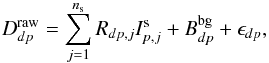 (A.1)where Rdp,j is the response of the instrument for source j (function of the incident angle of the source relative to pointing axis),
  is the flux of source j during exposure p and
  the background both recorded during the exposure p for detector d. ϵdp are the measurement errors on the data , they are assumed to have zero mean, to be independent, and to be normally distributed with a known variance σdp (
![Mathematical equation: \hbox{$\epsilon_{dp} \sim N(0,[\sigma_{dp}^2]) $}](/articles/aa/full_html/2013/07/aa19605-12/aa19605-12-eq174.png) and
and  ).
).
For a given exposure p, , ϵdp, Rdp,j, and are vectors of nd(p) elements (say, nd = 19) elements). However, nd(p) corresponds to the number of functioning detectors, the possible values are 16, 17, 18 or 19 for single events and up to 141 when all the multiple events are used in addition to the single events (Roques et al. 2003). For a given set of np exposures, we have to solve a system of M ( ) equations (Eq. (A.1)).
To reduce the number of free parameters related to the background, we take advantage of the stability of relative count rates between detectors and rewrite the background term as  (A.2)In this expression, either Ud or
  is supposed to be known, depending on the hypotheses made on the background structure. To illustrate the idea, suppose that Ud is known. U is an “empty field” (Bouchet et al. 2010), a vector of nd elements. Then, the number of parameters necessary to model the background reduces to np. The number of unknowns (free parameters) of the set of M equations is then (ns + 1) × np (for the ns sources and the background intensities, namely Is and Ibg). Fortunately, a further reduction of the number of parameters can be obtained since many sources vary on timescales longer than the exposure timescale. In addition, many point sources are weak enough to be considered as having constant flux within the statistical errors, especially for the higher energies. Then the np × ns parameters related to sources will reduce to
  parameters and, similarly, Nb for the background. As these parameters also have a temporal connotation, they are also termed, hereafter, “time bins”. Finally, we have
  free parameters to be determined. If the source and background relative intensities are supposed to be constant throughout all observations (time spanned by the exposures), omitting the detector index, the equation can be simplified as
 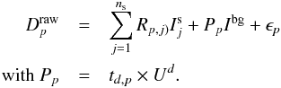 (A.3)Here Pp is a vector of nd(p) elements. The aim is to compute the intensities Is(j) of the ns sources and the background relative intensity Ibg. Therefore, the problem can be written in matrix form as
 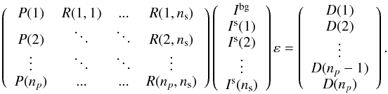 At last, Eq. (A.1) reduces to the general linear system H0x0 + ε = y, where H0 is the transfer matrix, y the data, ε the measurement errors and x0 the unknowns H0 (elements Hij) is an M × N0 matrix and N0 = ns + 1. x0 = (Ibg,Is(1),··· ,Is(ns))T is a vector of length N0. y = (D1,D2,··· ,Dnp)T and
  are vectors of length M. Now, if all N0 sources (here sources and background) are assumed to vary and the signal of source J is represented by nseg(J) piecewise constant segments of time or “time bins”, then each columns of H0 will be expanded in nseg(J) columns. Equation (A.1) reduces to Hx + ε = y, where the matrix H is of dimension M × N, with
  and x a vector of length N representing the intensity in the “time bins”. Schematically and to illustrate the purpose of Sect. 5.1, H can be derived from H0:
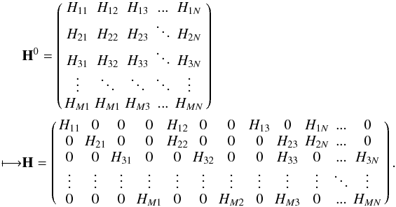 For the training data given in Sect. 2, which contain ≃39 000 exposures and for the 25–50 keV energy band, we used
 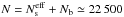 “time bins” (Bouchet et al. 2011). To fit the sky model consisting of sources plus instrumental background to the data, we minimized the corresponding chi-square value:
 ![Mathematical equation: \appendix \setcounter{section}{1} \begin{equation} \chi^2=\sum_{i=1}^{M} \left[ \frac{y_i-\sum_{j=1}^{N} H_{ij}x_j} {\sigma_i} \right]^2, \end{equation}](/articles/aa/full_html/2013/07/aa19605-12/aa19605-12-eq213.png) (A.4)where σi is the measurement error (standard deviation) corresponding to the data point yi, formally
(A.4)where σi is the measurement error (standard deviation) corresponding to the data point yi, formally  . By replacing H and y by their weighted version,
 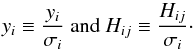 (A.5)The least-squares solution x is obtained by solving the following normal equation:
  (A.6)Here A is a symmetric matrix of order N, x and b are vectors of length N.
Appendix B: Segmentation/partition of a time series
Appendix B.1: Bayesian model comparison
The literature about model comparisons is vast, especially in the field of econometric (e.g. Zellner 1971; Poirier 1995; Koop 2003). We have some data y, a model Modeli containing a set of parameters θi. In our application, we have to choose between models of light curves (Model1 or Model2), based on observations over a time interval T: 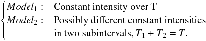 Using Bayesian inference (see for example Scargle 1998), the posterior odds ratio makes it possible to compare models i and j: it is simply the ratio of their posterior model probabilities:
  (B.1)where BFij is the Bayes factor comparing Modeli to Modelj. The quantity p(y | Modeli), the marginal likelihood
  (B.2)To compare Model2 with Model1, non-informative choices are commonly made for the prior model probabilities (i.e,
  ). Then, to prevent overfitting, we introduce a penalty parameter γ that chooses model Model2 instead of Model1 if
  (B.3)To fit the framework of expression Eq. (3), this equation can be equivalently rewritten as
 ![Mathematical equation: \appendix \setcounter{section}{2} \begin{equation} -\log [p(y | Model_2)] + \beta < -\log [p(y | Model_1)] \mathrm{~~ with~~} \beta=\log( \gamma). \end{equation}](/articles/aa/full_html/2013/07/aa19605-12/aa19605-12-eq233.png) (B.4)
(B.4)
Appendix C: Cost or likelihood function computation
Appendix C.1: Normal distributions
The model for the time series observations (Eq. (1)) is  where xi is the value measured at time ti, f is the unknown signal and ϵi the measurement errors. These errors are assumed to have zero mean, to be independent, and to be normally distributed with a known variance
  , thus the probability for bin i is
  The parameters associated with each segment are independent of each other, the likelihood can be calculated for the data within each segment or block. For the block K where the true signal is λ, the likelihood is,
  (C.1)The product is over all i such that ti falls within block K, for instance LK points fall into block K. We can simply maximize the likelihood for instance, PK = max(ℒ(K)); its maximum is reached for λ = λmax. With the following notations
  The expression can be written in terms of ordinary least-squares quantities:
 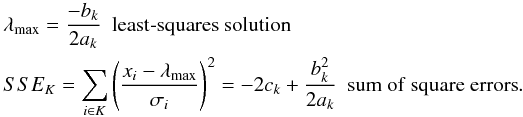 The block likelihood can be rewritten as
 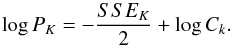 (C.2)Finally, the probability for the entire dataset is
 ![Mathematical equation: \appendix \setcounter{section}{3} \begin{equation} \log P= \log \left[ \prod_K P_K \right]= \sum_K {\log P_K}. \label{eqn:cost_series_marginalized} \end{equation}](/articles/aa/full_html/2013/07/aa19605-12/aa19605-12-eq246.png) (C.3)The choice of the prior of λ is another question, although many prior probabilities may be possible, we marginalize it by choosing the flat unnormalized prior (p(x | Model) = constant). If the variable λ is marginalized,
(C.3)The choice of the prior of λ is another question, although many prior probabilities may be possible, we marginalize it by choosing the flat unnormalized prior (p(x | Model) = constant). If the variable λ is marginalized,  (C.4)The expression can be integrated to give
 ![Mathematical equation: \appendix \setcounter{section}{3} \begin{equation} \log P= \sum_K \left[ -\frac{1}{2}\log a_K - \frac{SSE_K}{2} + \frac{1}{2} \log \pi+\log C_K \right]. \label{eqn:cost_series_flat_prior} \end{equation}](/articles/aa/full_html/2013/07/aa19605-12/aa19605-12-eq250.png) (C.5)
(C.5)
Appendix C.2: Generalization to multivariate normal distributions
We assume to have a linear regression model that assesses the relation between the dependent variables yi (the data) and the N-vector of regressors xi (unknowns). This relation is written in vector form as  (C.6)Thus, y is an M-vector, H an M × N matrix, ε an M-vector of errors, and x an N-vector. The errors are assumed to be independently normally distributed with mean 0 and a variance σ, that is
 ![Mathematical equation: \appendix \setcounter{section}{3} \begin{eqnarray*} {\vec \varepsilon} \sim N({\vec 0}_M,[{\bf \sigma}^2]), \end{eqnarray*}](/articles/aa/full_html/2013/07/aa19605-12/aa19605-12-eq255.png) where 0M is an M-vector of zeroes and [σ2] is an M × M diagonal matrix whose diagonal is
where 0M is an M-vector of zeroes and [σ2] is an M × M diagonal matrix whose diagonal is  . Using the properties of the multivariate normal distribution, it follows that the likelihood function is given by
 ![Mathematical equation: \appendix \setcounter{section}{3} \begin{equation} p({\vec y}| {\vec x}, {\bf \sigma})= \frac {1} {2 \pi^{M/2} \prod_{i=1}^{M} {\sigma_i} } {\rm e}^{-\frac{1}{2} ({\vec y}-{\bf H}{\vec x})'[\sigma^{-2}] ({\vec y}- {\bf H}{\vec x})}. \end{equation}](/articles/aa/full_html/2013/07/aa19605-12/aa19605-12-eq260.png) (C.7)The likelihood function can be rewritten in terms of ordinary least-squares quantities:
(C.7)The likelihood function can be rewritten in terms of ordinary least-squares quantities: ![Mathematical equation: \appendix \setcounter{section}{3} \begin{eqnarray*} \begin{split} & \hat {\vec x}= ({\bf H}'[{\bf \sigma}^{-2}]{\bf H})^{-1} {\bf H}^{\rm T} [{\bf \sigma}^{-2}]{\vec y} & \ \ \text{\small least-squares solution} \\ & SSE=({\vec y}-{\bf H} \hat {\vec x})^{\rm T}[{\vec \sigma}^{-2}] ({\vec y}-{\bf H} \hat {\vec x}) & \ \ \text{\small sum of squared errors}. \end{split} \end{eqnarray*}](/articles/aa/full_html/2013/07/aa19605-12/aa19605-12-eq261.png) If we take the highest likelihood value,
If we take the highest likelihood value, 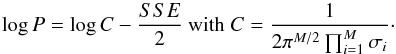 (C.8)If the variable x is marginalized by choosing the flat un-normalized prior, it yields for the marginal posterior after integration
 ![Mathematical equation: \appendix \setcounter{section}{3} \begin{equation} \log P=\log C + \frac{1}{2} \log \frac{(2 \pi)^p}{det ({\bf H}'[\sigma^{-2}]{\bf H} )} -\frac{SSE}{2}\cdot \label{eqn:cost_data_flat_prior} \end{equation}](/articles/aa/full_html/2013/07/aa19605-12/aa19605-12-eq263.png) (C.9)For M = L, N = 1 and H a matrix with elements Hij = 1, we recover Eqs. (C.2) and (C.4), with
(C.9)For M = L, N = 1 and H a matrix with elements Hij = 1, we recover Eqs. (C.2) and (C.4), with ![Mathematical equation: \appendix \setcounter{section}{3} \begin{eqnarray*} a= {\rm det} ({\bf H}'[{\bf \sigma}^{-2}]{\bf H})= \sum_{i=1}^{N} {\frac{1}{\sigma_i^2}}\cdot \end{eqnarray*}](/articles/aa/full_html/2013/07/aa19605-12/aa19605-12-eq267.png)
Appendix D: Common model selection criteria
Other penalty cost functions are possible, the most widely known criteria for model selection among a class of parametric models with different numbers of parameters are AIC (Akaike 1974) and BIC (Schwartz 1978). Given ℒ, the likelihood of the data, their expressions are AIC = 2k − 2log (ℒ), BIC = − 2 log ℒ + klog (M). Here M is the number of data and k the number of parameters used in the model. Both AIC and BIC fit the general form given in Eq. (3) with (β = 2) and (β = log M). The penalty term of BIC is more stringent than the penalty term of AIC (for M > 8, k × log M exceeds 2k). The AIC formula is based on an asymptotic behavior with M large and a small number of parameters k and BIC on an asymptotic approximation to a transformation of the Bayesian posterior probability of a candidate model. Thus, both are issued from asymptotic approximation and may have some drawbacks in some range of parameters. Modified versions of these criteria have also been developed to correct their main weakness. The Hannan-Quinn information criterion (HQC; Hannan & Quinn 1979) proposes something intermediate with (HQC = − 2log ℒ + 2klog (log M)) and (β = 2log (log M)).
Appendix E: Mathematical utilities
The formulas below avoid recomputing the inverse of matrix from scratch when a small rank adjustment is performed on the matrix.
Appendix E.1: Sherman-Morrison-Woodbury formula – inversion lemma
Suppose that one aims to invert the matrix A + UCV. Here A, U, C, and V are n × n, n × k, k × k and k × n matrices, respectively. UCV is called rank-k update (or correction) of A. If C has a much smaller dimension than A, it is more efficient to use the Sherman-Morrison-Woodbury formula than to invert A + UCV directly. Now suppose that A-1 has already been computed and that C and C-1 + VA-1U are invertible. The Sherman-Morrison-Woodbury formula says that the inverse of a rank-k correction of some matrix can be computed by applying a rank-k correction to the inverse of the original matrix. Alternative names for this formula are the matrix inversion lemma or simply the Woodbury formula. The Woodbury matrix identity is  The determinant of A + UCV is obtained through the relation:
Appendix E.2: Inverse of a partitioned matrix
Let the N × N matrix A be partitioned into a block form as below, where T and W are square matrices of size t × t and w × w, respectively (t + w = N). Matrices U and V are not necessarily square, and have size t × w and w × t, respectively. Let matrices T, W and Q = W − VT-1 being invertible. The inverse of A can be written as 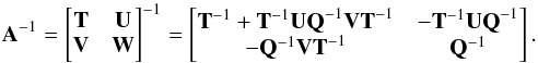 The determinant of A is obtained through the relation:
Appendix E.3: Application
We have to solve system Hx = y in the least-squares sense; y is the right-hand side, H a matrix and x the solution, see also Appendix A. Now, we need to update the solution x of the system of equations Ax = (HTH)x = HTy after adding or deleting some columns to H. Here H is a matrix of size M × N, x and y are vectors of length N and M, respectively. We first derive the expression of the updated inverse of A. We assume that the inverse of A is already computed and denote by A∗ the updated corresponding matrix. To simplify, we just plug the formula for 1 column added or suppressed. First we add Nadd columns to H such that H∗ = [Hv], v is a matrix of size M × 1 representing the newly added column, then 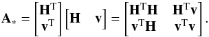 The inverse of this partitioned matrix is (Appendix E.2)
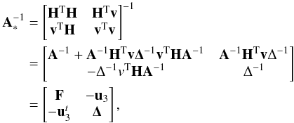
where Δ = vTv − vTHA-1HTv. Algorithm 1 performs the operation without accessing A-1 explicitly. We use the MATLAB notation “\” to denote the solution of a linear system (“x = A \ b′′ ≡ “x = A-1b′′): it emphasizes the fact that the system is solved without forming the inverse of the matrix of the system. If we need to remove a column from H, the algorithm is described in algorithm 2.
Appendix E.4: Adding Nadd columns and suppressing Nsub columns
The two algorithms described above are also applicable without loss of generality when several columns are added or removed. Algorithm 3 first adds Nadd columns and then suppresses Nsub columns from the transfer matrix H and updates the solution x∗ and predicted data  .
.
Appendix F: “Pseudo-codes”
The codes (simplified versions) for the ’image-space’ and ’data-space’ algorithms are written in IDL and Fortran, the time series of GX 339-4 (6.2.2) and the data for V0332+53 (6.3.1) that are to be used as input data to these codes can be downloaded at http://sigma-2/integral/algorithms. These codes and input data allow one to reproduce the main features of Figs. 4 and 10.
Appendix F.1: “Image-space” algorithm
Appendix F.2: “Data-space” algorithm
All Tables
Gain in time achieved by “source loop” parallelization of the “data-space” algorithm.
Mean time spent in the “source loop” by the “full” and “limited memory” versions of the ’data-space’ algorithm.
All Figures
|
Fig. 1 Flowchart of the “image-space” algorithm (pseudo-code in Appendix F.1). The vector last gives the starting point of individual segments of the best partition in the following way; let τm=last(L), τm − 1=last(τm − 1) and so on. The last segment contains cells (data points) τm,τm + 1,...,n, the next-to-last contains cells τm − 1,τm − 1 + 1,...,τm − 1, and so on. |
| In the text | |
|
Fig. 2 Flowchart of the “data-space” algorithm (pseudo-code in Appendix F.2). The cost function calculation, here the shaded box, is detailed in Fig. 3. |
| In the text | |
|
Fig. 3 Flowchart of the calculation of the cost function for the “data-space” algorithm. |
| In the text | |
|
Fig. 4 GX 339-4 intensity variations. The 26–40 keV IBIS time series (gray), which contains 1183 data points (one measurement per exposure), is segmented into 17 constant segments or “time bins” (green). The |
| In the text | |
|
Fig. 5 GX 339-4 time series segmentation. Variation of the |
| In the text | |
|
Fig. 6 Intensity variations of GX 339-4 and GX 1+4 in the 27–36 keV band as a function of the exposure number. The SPI segments are plotted in red and the IBIS raw light curves (26–40 keV) are drawn in gray. The segmented IBIS time series (scaled S/N) is shown in green. The count rate normalization between IBIS and SPI is arbitrary. |
| In the text | |
|
Fig. 7 “Image-space” method applied to GRS 1915+105. The intensity variations as a function of the exposure number are shown in the 27–36, 49–66, 90–121 and 163–220 keV band as indicated in the figure. The different bands are translated on-to the y-axis (the intensities are in arbitrary units). The SPI segments are plotted in red and the IBIS time series (scaled S/N) are drawn in gray (26–40, 51–63, 105–150, and 150–250 keV). The number of “time bins” deduced from the time series segmentation are 174, 50, 8, and 1. The global normalization factor in each energy band between the fluxes of the two instruments is arbitrary. |
| In the text | |
|
Fig. 8 IBIS/SPI flux correlation in 17, 2245, and 122 “time bins” for GX 339-4, 4U 1700-377, and GX 1+4. The red line is a straight-line fitting (with errors in both directions) with a chi-square of 25 (15 d.o.f.), 3961 (2243 d.o.f.), and 321 (120 d.o.f.). |
| In the text | |
|
Fig. 9 (Bottom) Reduced chi-square ( |
| In the text | |
|
Fig. 10 ‘’Data-space” method applied to V0332+53. The source intensity variations (25–50 keV) were modeled by nine segments (red) and were compared with the IBIS time series (26–51 keV, gray). The green curve corresponds to the IBIS flux averaged on SPI-obtained segments. The insert is a zoom between exposure number 81 and 179. (Top) SPI intensity variations model (black) compared with Swift/BAT time series (24–50 keV, purple line). The scale between the different instruments is arbitrary and was chosen such that their measured total fluxes are equal. It should be noted that the Swift/BAT and IBIS data are not necessarily recorded at the same time as the SPI data, nor exactly in the same energy band. |
| In the text | |
|
Fig. 11 Same caption as Fig. 10, but for GRS 1915+105 in the 27–36 keV band. The intensity linear correlation coefficients are 0.98 between IBIS (26–40 keV) and SPI, and 0.97 between Swift/BAT (24–35 keV) and SPI. |
| In the text | |
|
Fig. 12 Black denotes the SPI-IBIS correlation and green the SPI-Swift/BAT flux correlation in the “time bins” defined using the “data-space” method. The best SPI-IBIS and SPI-Swift/BAT linear regression are shown in red and purple. Left shows Cyg X-1 and right GRS 1915+105. |
| In the text | |
|
Fig. 13 Intensity evolutions (red) of IGR J17464-3213, GRS 1758-258, GX 1+4, GS 1826-24, and GX 354-0 in the 27–36 keV band. The IGR J17464-3213 dataset is divided in-to three subsets (dashed vertical lines show the limits) during the computation. The IBIS time series (30–40 keV) is shown in gray and the averaged fluxes in SPI “time bins” are plotted in green, as in Fig. 10. The distance of GRS 1758-258, GX 1+4, GS 1826-24, and GX 354-0 to IGR J17464-3213 are 7.3, 8.1, 12.7, and 3.4°. |
| In the text | |
|
Fig. 14 Comparison of GX 339-4 (27–36 keV) intensity variations obtained with the “image-space” and the “data-space” algorithms. The common SPI/IBIS database contains 1183 exposures. The “image space” method describes GX 339-4 intensity variations with 17 segments (red) for a |
| In the text | |
|
Fig. 15 “Data-space” algorithm has modeled the temporal evolution of GX 339-4 in the 27–36 keV band with 15 constant segments (blue). The light curve (in gray) of GX 339-4 was obtained by directly processing SPI data (after fixing the temporal evolution of the other sources). It contains 1183 data points (one measurement per exposure) The red curve is the segmentation of the gray curve into 15 segments with the “image space” algorithm. (*) If the background is forced to vary exposure-by-exposure, the GX 339-4 light curve is segmented only into six segments (dashed-green). |
| In the text | |
Current usage metrics show cumulative count of Article Views (full-text article views including HTML views, PDF and ePub downloads, according to the available data) and Abstracts Views on Vision4Press platform.
Data correspond to usage on the plateform after 2015. The current usage metrics is available 48-96 hours after online publication and is updated daily on week days.
Initial download of the metrics may take a while.