| Issue |
A&A
Volume 551, March 2013
|
|
|---|---|---|
| Article Number | A93 | |
| Number of page(s) | 21 | |
| Section | Extragalactic astronomy | |
| DOI | https://doi.org/10.1051/0004-6361/201220013 | |
| Published online | 28 February 2013 | |
Magellan/MMIRS near-infrared multi-object spectroscopy of nebular emission from star-forming galaxies at 2 < z < 3⋆,⋆⋆
1
Department of Astronomy, Oskar Klein CenterStockholm
University,
AlbaNova,
10691
Stockholm,
Sweden
e-mail:
lguai@astro.su.se
2
Pontificia Universidad Católica de Chile, Departamento de
Astronomía y Astrofísica, Casilla
306, Santiago 22,
Chile
3
Department of Physics and Astronomy, Rutgers, The State University
of New Jersey, Piscataway, NJ
08854,
USA
4
Université de Toulouse, UPS-OMP, IRAP, Toulouse, France
5
CNRS, IRAP, 14
avenue Edouard Belin, 31400
Toulouse,
France
6
Space Science Institute, 4750 Walnut Street, Suite 205, Boulder, Colorado
80301,
USA
Received: 11 July 2012
Accepted: 14 January 2013
Aims. To investigate the ingredients, which allow star-forming galaxies to present Lyα line in emission, we studied the kinematics and gas phase metallicity of the interstellar medium.
Methods. We used multi-object near-infrared spectroscopy with Magellan/MMIRS to study nebular emission from z ≃ 2−3 star-forming galaxies discovered in three MUSYC fields.
Results. We detected emission lines from four active galactic nuclei and 13 high-redshift star-forming galaxies, including Hα lines down to a flux of (4 ± 1)E-17 erg s-1 cm-2. This yielded seven new redshifts. The most common emission line detected is [OIII]5007, which is sensitive to metallicity. We were able to measure metallicity (Z) for two galaxies and to set upper (lower) limits for another two (two). The metallicity values are consistent with 0.3 < Z/Z⊙ < 1.2, 12 + log (O/H) ~ 8.2−8.8. Comparing the Lyα central wavelength with the systemic redshift, we find ΔvLyα − [OIII] 5007 = 70−270 km s-1.
Conclusions. High-redshift star-forming galaxies, Lyα emitting (LAE) galaxies, and Hα emitters appear to be located in the low mass, high star-formation rate (SFR) region of the SFR versus stellar mass diagram, confirming that they are experiencing burst episodes of star formation, which are building up their stellar mass. Their metallicities are consistent with the relation found for z ≤ 2.2 galaxies in the Z versus stellar mass plane. The measured ΔvLyα − [OIII] 5007 values imply that outflows of material, driven by star formation, could be present in the z ~ 2−3 LAEs of our sample. Comparing with the literature, we note that galaxies with lower metallicity than ours are also characterized by similar ΔvLyα − [OIII] 5007 velocity offsets. Strong F([OIII]5007) is detected in many Lyα emitters. Therefore, we propose the F(Lyα)/F([OIII]5007) flux ratio as a tool for the study of high-redshift galaxies; while influenced by metallicity, ionization, and Lyα radiative transfer in the ISM, it may be possible to calibrate this ratio to primarily trace one of these effects.
Key words: techniques: spectroscopic / galaxies: high-redshift / galaxies: star formation
This paper includes data gathered with the 6.5 m Magellan Telescopes located at Las Campanas Observatory, Chile
Tables 4−6 and Appendices are available in electronic form at http://www.aanda.org
© ESO, 2013
1. Introduction
Characterizing star formation at high redshift is critical for the investigation and understanding of galaxy formation and evolution. This task is often difficult, however, since distant star-forming galaxies can be quite faint and many of their characteristic diagnostic features redshifted into different observational regimes. The identification of high-redshift objects during specific evolutionary stages amidst foreground sources generally falls into two categories, either photometric methods which sample portions of the integrated spectral energy distribution (SED) or narrow-band imaging which select specific emission lines at specific redshifts.
Photometric methods (e.g., the Lyman break galaxy, or LBG, technique, Steidel et al. 1996; the Lyman alpha decrement, or BX technique, Steidel et al. 2004) have been extensively used to identify large samples of high-redshift galaxies, and even characterize their physical properties via comparisons to theoretical SEDs, generated by various initial mass functions, star-formation histories, stellar masses, dust reddening and interstellar medium (ISM) metallicities (e.g., Shapley et al. 2003; Pentericci et al. 2007). The advantage of the photometric techniques is that faint sources, occupying wide fields-of-view and wide redshift slices, can be detected, while the disadvantage is the lack of redshift confirmation.
A more efficient way to detect galaxies, at least in a narrow redshift range, is by using narrow-band filters covering a specific line wavelength at a specific redshift, such as Lyα (e.g., Cowie & Hu 1998). In principle Lyα could be observed up to z = 10 from the ground. Over the past decade, astronomers have built large samples of Lyα emitters (LAEs) at z > 2 (e.g., Rhoads et al. 2000; Gronwall et al. 2007; Ouchi et al. 2008; Nilsson et al. 2009). Narrow-band techniques have been used to detect Hα, [OII]3727 and [OIII]5007 line emitters at various redshifts (e.g., Thompson et al. 1994; Hayes et al. 2010b; Hatch et al. 2011; Shim et al. 2011). Such surveys, however, often require spectroscopic follow-up to weed out lower redshift emission-line galaxies which contaminate the samples. New multi-narrow-band surveys, with narrow-band filters covering Lyα, [OII]3727 and Hα+[NII] at z = 2.2 (e.g., Nakajima et al. 2012a; Lee et al. 2012), now have the advantage to reduce almost completely the contamination from low-redshift objects and also to calculate emission-line ratios, sensitive to galaxy metallicity.
In the context of the MUSYC survey (Gawiser et al. 2006)1, we amassed two samples of LAEs at z ≃ 3.1 and z ≃ 2.1. Their physical properties were studied by Gronwall et al. (2007), Gawiser et al. (2007), Lai et al. (2008), Guaita et al. (2010), Guaita et al. (2011), Acquaviva et al. (2012), and Bond et al. (2012), which found LAEs to be in the lower mass range of the mass distribution of star-forming galaxies (SFGs), observed during active phases of star formation, and characterized by low dust content and compact morphology. These are the ideal samples to constrain any evolution (or lack thereof) between redshifts of z ≃ 3.1 and z ≃ 2.1. Ciardullo et al. (2012) found z ≃ 3.1 LAEs with luminosities brighter than L(Lyα) > 1042.4 erg s-1 had almost twice the number density of z ≃ 2.1 LAEs in the Extended Chandra Deep Field South. Also, the number of galaxies with EW(Lyα) > 100 Å at z ≃ 3.1 was almost twice the number at z ≃ 2.1. While z ~ 3 LAEs were observed to be consistent with zero dust content (Gawiser et al. 2007; Nilsson et al. 2009; Ono et al. 2010), the SED fitting of LAEs at z ~ 2 showed a moderate amount of dust (Nilsson et al. 2011; Hayes et al. 2010a; Guaita et al. 2011).
The SED analyzes also showed that z ≃ 3.1 LAEs are low mass (108−109 M⊙), young galaxies (20 Myr) in active phases of star formation (Gawiser et al. 2007; Lai et al. 2008), while z ≃ 2.1 LAEs are instead characterized by more variety. For instance, some z ≃ 2.1 LAEs have “ages since star formation began” that are compatible with a few hundreds of Myr and the sub-sample of more massive galaxies (109.5 M⊙) are characterized by redder colors (e.g., Gu2011). This was interpreted as an indication that there are a wider variety of ISM mechanisms, due to the spatial and velocity distribution of dust and neutral Hydrogen at lower redshift, which could be responsible for the escape of Lyα photons (with delayed episodes of star formation among the proposals; Shimizu & Umemura 2010). A recent scenario was described in Acquaviva et al. (2012), who used a Monte Carlo Markov chain code (GalMC, Acquaviva et al. 2011) to derive physical parameters from the SEDs of our z ≃ 3.1 and z ≃ 2.1 LAE samples. They proposed that higher-redshift LAEs were on average more metal-poor, even if older, than lower redshift ones. The investigation of intrinsic properties and direct metalllicity estimations for individual galaxy could be very useful to confirm this hypothesis. Our current work here looks to address two main aspects of this scheme via estimates of the gas phase metallicity and an investigation of ISM kinematics. Star-formation activity and supernova explosions could be responsible for pushing material out of the galaxies in the form of outflows, which consequently leave imprints in the profile of Lyα emission (Verhamme et al. 2006).
Log of Nov. 2010 and May 2011 runs.
The estimation of metal line abundances is important to increase the statistics of metallicity estimations in SFGs at high redshift. While Balmer emission lines can be modeled by stellar synthesis codes (Schaerer & de Barros 2012), a deeper investigation of the [OIII] emission relative to the Hydrogen lines is useful to allow better SED modeling of optical emission lines. Notably, strong [OIII]5007 emission can comprise a significant fraction of the K band magnitude at z ~ 3 (McLinden et al. 2011), making its characterization critical for the correct interpretation of broad-band photometric properties. Moreover, McLinden et al. (2011) and Finkelstein et al. (2011) recently showed that significant velocities offsets between Lyα and systemic redshift as measured by [OIII] can be present in LAEs, which are clearly important for an interpretation of the Lyα emission.
This pilot project focuses on obtaining rest-frame optical spectra for a sizeable sample of high-redshift galaxies via near-infrared multi-object spectrographs (NIR-MOS). Only a few NIR-MOS instruments have been available to date. NIR spectra have been obtained by using the multi-object infrared camera and spectrograph (MOIRCS) at the Subaru telescopes to observe cluster stars (e.g., Scholz et al. 2009), medium redshift massive galaxies (e.g., Onodera et al. 2010; Hayashi et al. 2011), BzK galaxies with KAB ≤ 22 (Yoshikawa et al. 2010), Hα emitters (Tanaka et al. 2011), and quasars (Del Moro et al. 2009). Recently the MMT and Magellan Infrared Spectrograph (MMIRS) was used to obtain NIR spectra of LAEs at z ≃ 2.2 (Hashimoto et al. 2013) with relatively bright optical and NIR magnitudes (at least compared to those observed here).
We present here a new NIR spectroscopic survey, with five main aims:
-
1)
to demonstrate the capabilities for studying faint emission-linegalaxies with MMIRS on the Magellan Clay 6.5 m telescope;
-
2)
to confirm redshifts of photometrically-selected SFGs;
-
3)
to measure rest-frame optical emission line ratios and estimate metallicities of galaxies undergoing active phases of star formation;
-
4)
to place SFGs, previously detected via Lyα or Hα emission lines, in an evolutionary sequence and investigate similarities and differences with respect to continuum-selected SFGs in the same redshift range;
-
5)
to probe the gas kinematics of LAEs in order to study channels of the escape of Lyα photons.
We adopt AB magnitudes throughout, following the Two Micron All Sky Survey (2MASS) zero-point magnitudes, KAB = KVega + 1.87.
When we refer to the rest-frame wavelength of emission lines, we use vacuum-wavelengths of λLyα = 1215.67 Å, λ[OIII] 5007 = 5008.239 Å, λHα = 6564.614 Å. We denote the stellar reddening as E(B − V) and the nebular reddening as Eg(B − V). We assume a ΛCDM cosmology consistent with the WMAP 5-year results (Dunkley et al. 2009, their Table 2), adopting mean parameters of Ωm = 0.26, ΩΛ = 0.74, H0 = 70 km s-1 Mpc-1, σ8 = 0.8.
2. Observations and sample definition
MMIRS is a near-IR imager and multi-object spectrograph with a 4′ × 6.9′ field-of-view2, operating on the Magellan Clay telescope since the end of 2010. Mask design followed the MMT mask preparation procedure3. The objects studied in this paper come from two two-night observing runs in late 2010 and mid 2011 (see Table 1). Weather conditions and instrument performance were more favourable in the first run. Two entire nights were allocated in Nov, while only half nights in May, 19th and 20th. The half nights allocated to the second run resulted in airmasses that were generally higher than the first run, reaching up to airmass 2.0 on May 20th.
We obtained spectra in three fields belonging to the MUSYC survey (Gawiser et al. 2006, hereafter Ga2006): two masks in the ECDF-S (Extended Chandra Deep Field South), one mask in the EHDF-S (Extended Hubble Deep Field South), and one mask in the SDSS-1030 region.
Sources detected in MMIRS survey.
List of sources showing emission lines in each mask.
In Table 2 we show the number of detected sources versus the targeted ones. In Table 3 we list the 17 sources from which we detect emission lines. The names designed in Col. 1 will be used hereafter. When filling the masks we chose three main categories of sources:
-
1)
Narrow-band selected LAEs from Gronwall et al. (2007;hereafter Gr2007) at z ≃ 3.1 and in Guaita et al (2010; hereafter Gu2010) at z ≃ 2.1. Also, we considered Lyα and/or Hα emitters detected by Hayes et al. (2010) in their double blind (DB) survey. The detected sources originally belonging to this category and studied here are LAE27, z3LAE2, z2LAE2, z2LAE3, DB8, DB12, and DB22 (Table 3 notation).
-
2)
SFGs as defined in Ga2006 and Guaita et al. (2011), and studied in Berry et al. (2012), selected using the broad-band color drop-out technique at z ~ 3 (LBGs) and Lyα decrement at z ~ 2 (“BXs”). The detected sources originally belonging to this category and studied here are BX1, BX4, BX10, BX14, BX16, and LBG11 (Table 3 notation). Our spectroscopy revealed the presence of Lyα emission with equivalent widths larger than 20 Å for BX1 and BX10, confirming them as LAEs. Also included in this category were BzK galaxies either from Blanc et al. (2008) with KAB < 22 or, in the case of Bzk25, selected from deeper VLT infrared spectrometer and array camera (ISAAC) imaging with fainter continua (Mark Dickinson and Jeyhan Kartaltepe, private communication). The latter was not expected a priori to present any continuum in the NIR.
-
3)
Active galactic nuclei (AGNs) expected to lie in the range 2 < z < 3 and show strong rest-frame optical lines, selected from optical (Francke et al. 2008), radio (Miller et al. 2008), or X-ray catalog (Xue et al. 2011). The AGNs originally belonging to this category and studied here are AGN5 and AGN26.
We designed the MMIRS masks giving first priority to Lyα/Hα emitting galaxies observed at z ≃ 2 and z ≃ 3.
Galaxies selected to be either Lyα and/or Hα emitters were expected have faint continua and only display a few emission lines in the NIR spectra like [OIII] and Hα due to star formation. NIR spectra of DB sources, where Hα fluxes were measured photometrically, are very important for setting upper limits on Hα detection. We filled in the remaining space on the masks using SFGs and AGNs with or without firmly known redshifts but suspected to lie at z ≥ 1.5. We also included low-redshift galaxies, which were expected to yield strong continuum and thus be useful tests of MMIRS’ capability, as well as slit stars for mask alignment phase and flux calibration. In each of the four masks we included 3−4 square boxes with alignment stars, although during the second run we used three additional stars for flux calibration and additional alignment checks.
Our z ≃ 2.1 and z ≃ 3.1 LAE samples had a median Lyα flux of 4.0 × 10⁻¹⁷ erg s-1 cm-2 (Gr2007, Gu2010). The Lyα/Hα ratio can be significantly reduced from the theoretical value of 8.7 for case B recombination (Osterbrock 1989) even by a small amount of dust reddening. To produce a reasonable estimate of the reddening expected, we assumed a Calzetti law with E(B − V) = 0.04, which is typical of our sample LAEs (Ga2007, Gu2011), and that Lyα photons experience the enhanced dust attenuation of nebular gas but no further amplification of dust column from radiative transfer. This predicts a Lyα/Hα ratio of ~3, implying a median Hα flux for our sample of 1.3 × 10⁻¹⁷ erg s-1 cm-2. Scaling from the predicted S/N per resolution element for the current HK grism (MMIRS S/N calculator4), we anticipated a S/N of 6 in 4 h for the lines predicted in our typical LAEs. We obtained total exposure times of 4.8 and 4.7 h for our two ECDF-S masks, and 3.2 and 2.7 h for our SDSS and EHDF-S masks, respectively. Spectra were taken through the HK grism and H + K filter covering 1.25−2.45 μm wavelength range, through a slit with width equal to 0.7′′ (0.5′′ for a few sources in ECDF-S masks). The filter transmission has the same throughput of 70% at 16 000 and 21 000 Å. At 19 000 Å the throughput has its maximum, but the atmospheric absorption is maximum at this wavelength as well.
During the Nov run we chose a dithering pattern of 0, 3, −2, 2, −3 arcsec along the slit length to perform a better sky subtraction. However, the shift of pair subtracted images could cause an overlap of close-by slits (Sect. 3). Also, a 3′′ dither caused alignment stars to move outside of their boxes in a few cases. Therefore, we adopted a 0, 2, −2 pattern in the May run. We re-aligned the masks frequently during the nights, typically after a series of 5−10 science frames. We observed telluric standard stars5 2−3 times per mask per night, placing the telluric in 5 slits across the mask to achieve full spectroscopic coverage.
MMIRS is characterized by a 0.2012′′/pixel scale. It corresponds to a 3.5 (2.5) pixel resolution element for a 0.7′′ (0.5′′) slit width. For a sampling of 7 Å/pixel, this means a line resolution of 25 (18) Å and a resolution R = 800 (1100) at λ = 20 000 Å.
3. Reduction
A full account of our reduction procedure is reported in the Appendix A, while here we describe only the main details.
We used the mmfixen code provided by the MMIRS instrument scientific team6 to collapse all the information enclosed in the multi-extension files. The output became a new multi-extension file, in which the 1st extension was the science frame normalized to counts/s.
To calculate the wavelength calibration map we used the COSMOS7 public software package, which was originally designed to reduce optical multi-object spectra obtained with the Magellan IMACS and LDSS instruments and updated to work with NIR MMIRS data. Positional files (*.SMF) were generated for each mask by the MMIRS team (and mmirs2smf.py code) to make MMIRS mask frames compatible with COSMOS. We obtained a rough wavelength map using COSMOS align-mask and adjust-offset codes and then a final solution running COSMOS adjust-map.
The most prominent features in our NIR spectra were the atmospheric sky lines. They were used as a reference for the wavelength calibration, but afterwards they were eliminated from the science frames using an ABBA source offset procedure. We first subtracted two frames, A and B, adjacent in time to remove the bulk of the constant and variable IR backgrounds, obtaining background-subtracted (A-B) or (B-A) frames. Depending on the sky variation at a specific moment of the night and airmass, in the A-B and B-A frames sky lines are reduced by about 50−80%. We then applied offsets to align the dispersed source spectra from the A and B frames and summed the signals of aligned frames of the same mask for the entire run. The shift was determined based on the input dithering pattern. The remaining sky line residuals were due to rapid temporal sky line variations and variations along the slit for individual lines. These variations dominate the background noise.
We then applied the previously calculated wavelength map to the completely reduced frames. This was performed using the routine COSMOS extract-2dspec, which applies the wavelength map and and splits a multi-slit frame into individual slit 2D spectra. We used the IRAF twodspec.apextract.apall task to extract 1D spectra.
Giant A0 stars (without strong features in their NIR spectra) were used as flux standards to generate the sensitivity function needed for flux-calibrating science frames, as well as to correct telluric absorption features.
We chose extraction apall apertures of ±3 (±5) pixels for extracting 1D standard and science source spectra, respectively. The fractional missing flux due to the wings of the PSF falling outside the extraction aperture (not to be confused with slit losses) is estimated to be less than 10% in both the runs.
In the case of the Nov run, we compared our flux calibration for emission lines from AGN5 to those reported in the literature by van Dokkum et al. (2005); see Sect. 5 for more details. In the case of the May run, we compared the obtained sensitivity functions for our slit stars with their literature magnitudes, finding good agreement.
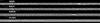 |
Fig. 1 2D spectra of AGNs detected in the 4 masks, all characterized by KAB > 20. The spectra are aligned in wavelength. Poisson noise due to sky emission line residuals can be seen as black vertical stripes. |
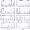 |
Fig. 2 Observed 1D spectra of AGNs in grey and best fit in red. From the top AGN5, BzK25, AGN26, z2LAE3. Vertical dashed lines represent the wavelengths of sky line residuals. The blue curve is the sky spectrum by Rousselot et al. (2000), which indicates the relative intensity of the OH emission lines. It has been scaled according to the panel axis to be visible. [OIII] doublet (Hα) wavelength ranges are presented in the left (right) panels. |
4. Emission line fitting procedure
After extracting 1D spectra, we fitted emission lines and continua with the python scipy optimized.leastsq function. The parameters of the fit were central wavelength (λ0), dispersion (σGauss), and amplitude (AGauss) of a Gaussian curve (![\hbox{$f_{\lambda} = (A_{\rm Gauss}/\sqrt{2\pi}) \exp[-(\lambda-\lambda_0)^2/2\sigma_{\rm Gauss}^2]$}](/articles/aa/full_html/2013/03/aa20013-12/aa20013-12-eq97.png) ) for emission lines and intercept of a flat continuum.
) for emission lines and intercept of a flat continuum.
To easily identify the first-guess fitting parameters we smoothed all raw spectra by a ~30 Å box. We performed a linear fit to the smoothed continua at ~16 000 Å and ~21 000 Å, excluding emission line wavelength regions from the continuum fit. We fitted the smoothed-spectrum continuum-subtracted Hα and [OIII]5007 emission lines with single Gaussians to measure λ0 (hence the source’s redshift) and the first-guess σGauss and AGauss.
We performed the fit a second time to obtain best-fit σGauss (σGauss, best−fit) values for three Gaussians fitted to Hα+[NII] doublet simultaneously, fixing the redshift inferred from λ0 in the previous step and varying σGauss and AGauss around the first-guess values. We fixed the ratio of the [NII] lines to 1:3 (Osterbrock 1989). Even if [NII] is not clearly seen in the 2D spectrum, this procedure was important to estimate the contribution of [NII] blended to Hα. Atek et al. (2011) found that the [NII] doublet contribution to Hα was on average 8% in their sample. We similarly fitted the [OIII]doublet + Hβ with three Gaussians, where we fixed the [OIII]doublet ratio to 1:2.98 (Storey & Zeippen 2000). We excluded pixels strongly contaminated by sky-line residuals from the fit.
After obtaining the best-fit λ0 and σGauss, best−fit for the six emission lines in the smoothed spectrum, we fixed these values and searched for the best-fit AGauss (AGauss, best−fit) in the raw spectrum. From this last amplitude estimation we calculated the integrated line flux (F(line) =  ). We estimated the 1σ uncertainty on the λ0, σGauss, best−fit, and AGauss, best−fit values assuming a single parameter of interest, calculating the diagonal elements of the fit covariance matrix.
The [OIII] doublet was a robust feature to find because it is composed by two separate emission lines with a known flux ratio. If we saw [OIII], but not Hα, we assumed an Hα upper limit of twice the continuum root-mean-square (rms) error at the wavelength of Hα multiplied by the MMIRS resolution of 25 Å. The same method was applied in the case we detected Hα but not [OIII].
4.1. Uncertainties of the emission line parameters
To estimate line integrated flux uncertainty, we used the parameter uncertainty derived from the best fit covariance matrix (Sect. 4). However, additional factors could increase the total error budget.
We performed a few tests to verify the goodness of the reduction and calibration processes. We calculated the observation point spread function (PSF) by measuring the median full width half maximum (FWHM) of the telluric standard spectral profile. Because telluric standards were observed in 5 slits along the mask spatial axis, we could estimate the average PSF variation along the mask. In addition to this, we could estimate the possible variations of the FWHM spectral profile with time in the series of 5 sub-sequent exposures. This could be related to the alignment, which might have varied with time. But in a series of five 1 s-long exposures, ΔFWHM was just 0.1′′. We did the same test considering the spectral profiles of stars in the science masks as well. The FWHM and the ΔFWHM are comparable to the ones measured for telluric stars. In the Nov run, for example, FWHM = 0.8′′ ± 0.2′′ for telluric and science frames. This means that our flux calibration could compensate for slit losses, in the case extraction aperture and slit width were the same for telluric and science spectra. The fraction of the flux in the wings of the spectral profile ending outside the extraction aperture should be less than 10%.
Flux calibration uncertainties are estimated to be less than 10% in the Nov masks and up to 30% in the May masks. This was produced by the standard deviation of the flux among standard spectra taken from the same slit along the run, due to changes in weather conditions.
Sky line residuals could also affect the integrated flux estimation. We avoided significant pixels with residual emission from the sky in the line fitting. In the case of [OIII], the presence of a doublet and a fixed ratio 2.98:1 compensated for the potential increase/decrease of flux due to sky line residuals.
Depending on the night seeing/slit width, sky emission lines can be broadened, producing an uncertainty in the wavelength calibration and so in the observed line center as well. The wavelength map needed to wavelength calibrate our spectra was successfully generated through the COSMOS package, but an uncertainty of 10 Å is the upper limit in the wavelength uncertainty due to broadened sky lines. To estimate this value, we extracted sky spectra from random slits of a few science frames, in which the ABBA procedure was not applied yet. We also average combined all these science frames the same way the final reduced ones were combined and extracted the sky spectrum from the combination. Then we compared the emission line wavelengths with the tabulated ones.
All these uncertainties are included in central wavelength and integrated line flux total error budgets, reported in the following figures.
5. Sources detected in MMIRS spectra
In Table 3 we list the 17 sources, for which we detected emission lines (Hα and [OIII]5007 have signal-to-noise ratio, S/N ≥ 3). AGNs, LAEs, and DB galaxies had the highest fraction of successful detections. The main reason for the low fraction was that the sources were generally faint in K band and that in some cases a particular emission line was overlapped with a strong sky line residual.
Several of the targetted AGNs exhibited strong, broad emission lines clearly seen in their 2D spectra (Fig. 1). Therefore, these sources were good candidates to test the sensitivity and capability of MMIRS, as described below. In Fig. 2 we show the AGN spectra in black and we over-plotted the best fit Gaussian curve in the [OIII] and Hα wavelength region as red curves. The blue spectrum is the sky spectrum from Rousselot et al. (2000). Figure 3 shows the line flux ratio diagram from Kewley et al. (2001) where SFGs appear to be separated from AGNs (upper left side in each panel). We used this diagram (originally proposed by Baldwin et al. 1981) to either identify and/or confirm AGNs among our sources.
5.1. Active galactic nuclei
AGN5 was previously studied in (van Dokkum et al. 2005, hereafter vD05), using Gemini/GNIRS. They used the GNIRS short camera with 32 lines mm-1 and 0.68′′ wide, 6.2′′ long slit. Their total exposure time was ~5500 s, with a seeing of ~0.7′′. We used a 0.5′′ slit in the H + K grism configuration for a total exposure time of 17 280 s (4.8 h). The estimated total spectroscopic throughput is ~30% in K and ~35% in H. This afforded us the chance to cross-check the performance of MMIRS against high-quality Gemini/GNIRS data. We mentioned before that our flux calibration was able to compensate for slit losses. By definition it also accounted for telescope aperture and system efficiency. However, for this object we needed to take into account an additional slit loss due to a narrower slit of 0.5′′ during a night with 0.8′′ seeing. This implied that we needed to increase the integrated flux by about 20% to compare with van Dokkum’s results. As described in the previous section, we fitted the continuum-subtracted emission lines with Gaussian curves to obtain the integrated flux and its uncertainty, after correcting for slit losses. Sky emission line residuals at 16 128 Å were excluded from the fit of the [OIII] doublet and we obtained F([OIII]5007) = 32.5 ± 6.7 E-17 erg s-1 cm2, F([OIII]4959) = 10.9 ± 2.3 E-17 erg s-1 cm2. Faint sky lines lying in the middle of the Hα+[NII] complex at 21 116 and 21 156 Å might still affect the results. We measured F(Hα) = 28.1 ± 7.9 E-17 erg s-1 cm2. The continuum rms in the [OIII] and Hα wavelength ranges are not significantly different.
Considering a PSF variation (ΔFWHM) of the order of 0.2′′ during the run and a flux calibration uncertainty of 10%, the MMIRS line flux measurements are consistent with the ones obtained using GNIRS by vD05 (F([OIII]4959) = (10.0 ± 1.0) E-17 erg s-1 cm2, F([OIII]5007) = (24.0 ± 2.4)E-17 erg s-1 cm2, and F(Ha) = (24.0 ± 2.4)E-17 erg s-1 cm2).
The squares in the upper and lower panels of Fig. 3 represent our estimations of line ratios for AGN5 (filled) and previous van Dokkum’s (open). Even if Hβ has very low S/N in our spectrum and so [OIII]/Hβ ratio is consistent with an upper limit, AGN5 appear to be located in the AGN region of the diagram.
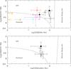 |
Fig. 3 Line ratio diagrams as presented in Kewley et al. (2001) (solid lines). The solid lines divide AGNs from Starburst galaxies. Symbols indicate AGNs found in our survey as explained in the text, the filled (open) squares are our (van Dokkum et al. 2005) ratio estimations for AGN5, the black triangle (pentagon) represents Bzk25 (AGN26), the red star z2LAE3. SFGs located in the region typical of Starbursts are presented for comparison: DB12 as a magenta circle, BX16 as a cyan star, and the two LAEs from Finkelstein et al. (2011) as orange dots. |
BzK25 was originally selected as a BzK galaxy. A public optical spectrum was available from the GOODS VIMOS survey (GOODS_LRb_002_1_q4_79_1.spec, Quality A optical redshift of 2.1449, Balestra et al. 2010)8.
This showed CIII]1909 and a weak HeII in emission. This spectrum might indicate it was an AGN, although CIV and NV were not formally detected (we note there is a faint line at the location of CIV which appears to have a P-Cyg profile; such features can be observed for SFGs). The MMIRS spectrum did not show any continuum, but showed [OIII] and Hα emission lines (S/N([OIII]) = 7, S/N(Hα) = 10). The filled triangle in Fig. 3 represents this source and supports the idea it is an AGN. Looking at Fig. 2 we can see sky lines are not significantly affecting Hα or [OIII]5007.
AGN26 is represented by the open pentagon in Fig. 3. The line ratio diagram, we chose to show here, indicates it is an AGN. The [OIII] doublet is not affected by sky emission lines, but sky line residuals could affect the [SII] integrated flux. The red star corresponds to z2LAE3. Even if it was initially selected as LAE through narrow-band technique in EHDF-S, it appeared to be an AGN based in Fig. 3 line ratios. It is the brightest source of the sample, with L(Lyα) was equal to 1043.5 erg s-1 (F(Lyα) ≃ 1.0E-15 erg s-1 cm2 and EW(Lyα)rest−frame = 74 Å) and it was the brightest source of the LAE sample in EHDF-S.
For comparison, we show BX16 and DB12, which fall in the Starburst region of the diagram, as well as LAEs from Finkelstein et al. (2011). However, we note that the most massive and most Lyα luminous galaxies are generally found near the border of AGN and Starburst regions.
5.2. Star-forming galaxies
We adopted the same procedure described in Sects. 4 and 5 for fitting continuum and emission lines of all the sources listed in Table 3 and showed in Figs. 4 and 5. The SFGs detected in our MMIRS spectra showed an average KAB magnitude of 22.3. We were not able to detect either emission lines nor continua from BzK galaxies fainter than KAB = 23 or photometrically selected LAEs with L(Lyα) fainter than 1042.94 erg s-1. The most prominent emission line observed is [OIII]5007 (typical S/N = 3−5), which is very intense in SFGs (Schaerer & de Barros 2012) and easy to identify thanks to its doublet. In Table 4 we report line fluxes, redshift, observed-frame equivalent width, and luminosities. This information was used to characterize the properties of SFGs in our sample.
5.2.1. Physical properties
In the past six years our sample of SFGs at 2 < z < 3 was studied via photometry and optical spectroscopy. In Gu2011 we fitted their stacked SED and showed that stellar mass and reddening were the only parameters we were able to constrain with high significance. We found that the median stacked SEDs were able to reproduce the median stellar E(B − V) and mass values of a sample, we defined as the typical ones. We accounted for the spread in the sample population by using the boot-strapping method to evaluate the uncertainties. It was also pointed out that stacking increased the signal-to-noise of ground-based photometric SEDs and revealed typical properties of our LAE samples. We needed LAE sub-samples (based on rest-frame UV magnitude, color, Lyα equivalent width, and brightness at observed-frame 3.6 μm separations) to identify unusual galaxy properties different from the typical ones.
Among GOODS VIMOS public spectra (Popesso et al. 2009; Balestra et al. 2010), we found that BX1 and BX10 were characterized by EWrest−frame(Lyα) > 20 Å and BX16 was characterized by Lyα in absorption. Thanks to MUSYC VIMOS and IMACS rest-frame UV spectra, LAE27 and z3LAE2 were confirmed to be LAEs, while LBG11 showed EWrest−frame = 8 Å (Fig. 4). In Table 6 we reported Hα/Hβ, Lyα/Hα, and Lyα/[OIII]5007 line ratios for all the SFGs of our survey. The integrated line fluxes were obtained by fitting MMIRS spectra shown in Figs. 4 and 5.
 |
Fig. 4 Observed-frame 1D spectra (black curve) of the sources showing either Lyα in emission or in absorption in rest-frame UV spectra. In red we show the best fit model spectra. From the top BX1, BX10, LAE27, z3LAE2, BX16, LBG11. The first, second and third panel columns represent Lyα (from MUSYC and GOODS-VIMOS surveys), [OIII]doublet and Hα wavelength ranges respectively. Dashed vertical lines indicate the wavelength of sky emission lines, which could leave residuals in the science spectra. Horizontal dashed blue lines indicate the continuum rms in the wavelength range where we did not see an expected emission line. As LAE27, z3LAE2, and LBG11 are at z ~ 3, Hα line would fall outside the MMIRS coverage. The rest-frame optical emission lines are unresolved. |
For the objects with available rest-frame UV spectra, a good (stellar) reddening estimation could be obtained from the β slope of he rest-frame UV continuum. This is shown as E(B − V)β in Table 6. Following Calzetti et al. (2000), β is related to E(B − V) through the following equations,  where A(1600) corresponds to the galactic absorption in magnitude at λrest−frame = 1600 Å, Eg(B − V) is the reddening of nebular gas, and E(B − V) that of stellar continuum. The constant c corresponds to a factor 0.44 ± 0.03 in Calzetti et al. (2000). However, the Calzetti law was calibrated at low redshift and there are recent works showing that factor could be just c = 1 at z ~ 2 (Erb et al. 2006). Hayes et al. (2010a) assumed c = 1 as well, because they noticed that c = 0.44 significantly over-predicts the SFR(Hα) with respect to SFR(UV) for their sample. For our sample, SFR(Hα) and SFR(UV) are within a factor of 2. From the SED fitting results in Gu2011, we also noted that 0.44 < c < 1 seemed to be more appropriate to reproduce SFRs, but we could not estimate one precise value. It is beyond the scope of this paper to investigate if c is closer to 0.44 or 1, so we assumed the Calzetti law entirely. Of course to dust-correct emission line fluxes we used Eg(B − V).
An alternative way to estimate dust reddening is the Balmer decrement (F(Hα)/F(Hβ) Miller & Mathews 1972). However, the low signal-to-noise Hβ line makes this an estimation which is less reliable than the previous ones. We reported the Balmer decrements and the implied stellar color excess, E(B − V)β − α, for 4 sources in Table 6.
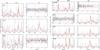 |
Fig. 5 Observed 1D spectra (grey curves) of the SFGs detected in our survey, without spectroscopic rest-frame UV counterparts (DB8, DB12, DB22, z2LAE2, BX4, BX7, BX14). [OIII]doublet and Hα regions are shown. If only one of these is detected, red vertical dashed lines indicate the location of Hα ([OIII]5007) lines which would be implied by the detected-line redshift for DB8, DB22, z2LAE2 (BX4). Dashed grey vertical lines indicate the wavelength of sky emission lines, which could leave residuals in the science spectra. Horizontal dashed blue lines represent the continuum rms in the wavelength range where we did not see an expected emission line. |
We considered the stellar dust reddening from stacked SED fitting as the most robust measure to use for dust reddening correction, when a rest-frame UV fit could not be performed. Therefore, we referred to the sub-sample definitions in Lai et al. (2008) and Gu2011 to infer stellar mass and E(B − V) from their SED fits. The categories, presented in those works and considered for the current analysis are IRAC-faint (f3.6 μm < 0.3 μJ), IRAC-bright (f3.6 μm ≥ 0.3 μJ), UV-faint (R ≥ 25.5), UV-bright (R < 25.5) LAEs, “BX” and LBGs. The z ~ 2 LAEs detected in our MMIRS survey all had SEDs consistent with those of UV-bright LAEs (log (M/M⊙) = 9.1[8.9−9.4], where square brackets correspond to the 68% confidence level range of stellar-mass values). The ones at z ~ 3 all belonged to the IRAC-bright sub-sample (M∗ ~ 109−1010 M⊙). The stacked sub-sample SED stellar mass was then rescaled to match the R band magnitude of individual sources. The SED for individual objects, performed in Hayes et al. (2010a), addressed stellar mass and reddening of DB sources. In Table 6 we reported the physical parameters from the SED fitting as E(B − V)SED and log (M∗/M⊙). Their error bars accounts for the spread in the sample population (Gu2011).
To infer star formation rate (SFR) of SFGs and LAEs, we applied the Kennicutt (1998) equation.
 Only for three sources (BX1, BX10, BX16) we were able to estimate E(B − V)β (and so Eg(B − V)β), we used to estimate SFRcorr(Hα). On the other hand Hα flux was an upper limit for the BX10 spectrum and it translated into an upper limit of SFRcorr(Hα). In the case of BX4, BX7, BX14, and DB12, the SFR(Hα) was assumed to be a lower limit of the SFRcorr(Hα) given the uncertain correction factor. On average SFRcorr(Hα) was found to be within a factor of two of the value estimated from the rest-frame UV.
As an example of the quantities introduced above, we present here the calculation relative to BX1. It was characterized by a quality A spectrum in GOODS survey. Fitting the spectroscopic rest-frame UV continuum with a power law, fλ ~ λβ, we obtained βbest fit = −1.6 ± 0.11 and so E(B − V)β = 0.12 ± 0.02, Eg(B − V)β = 0.27 ± 0.04. The Balmer decrement is measured as F(Hα)/F(Hβ) = 2.6 ± 2.5 i.e. F(Hα)/F(Hβ) ≤ 5.1, which implies Eβ − α ≤ 0.63. Its stellar reddening is then E(B − V)β − α ≤ 0.54, roughly consistent with the SED estimation, but not very conclusive.
BX1 was originally selected to have R = 24.65 and it belonged to the UV-bright LAE sub-sample (the R band magnitude of the stacked UV-bright sub-sample SED is 25.0). We, therefore, assumed the stacked SED shape was representative of this object, but we rescaled by a factor 1.4 the stellar mass to account for the individual object having a brighter R mag, yielding log (M/M⊙) = 9.25 [9.05−9.55].
Assuming E(B − V)β = 0.12 ± 0.02 and a Calzetti law for dust attenuation, we calculated Fcorr(Hα) = (9.4 ± 2.1) E-17 erg s-1 cm2 and SFRcorr(Hα) = 28.5 ± 8.2 M⊙ yr-1. This value was roughly consistent with the SFR averaged over the last 100 Myr found in Gu2011 for UV-bright LAEs (⟨ SFR ⟩ 100 = 10 [6−70] M⊙ yr-1). Following the Kennicutt (1998) equation for the SFR implied by the ultraviolet continuum, BX1 is characterized by an SFRcorr(UV, R band) around 50 M⊙/yr.
5.2.2. Line velocity offset
In the attempt to measure SFG properties we also studied ISM kinematics. [OIII]5007 can be used as a proxy of the galaxy systemic redshift (McLinden et al. 2011; Finkelstein et al. 2011). Fitting Lyα (from either GOODS or MUSYC spectra) and [OIII]5007 (from MMIRS spectra) emission lines with Gaussian curves we obtained best fits for their central wavelengths. To compare GOODS with our redshifts, we first applied the heliocentric correction at the time of the observations. It was v = + 22.2 km s-1 at Cerro Paranal and v = + 16.7 km s-1 at Las Campanas for BX1, as an example. Then, the offset velocity is estimated with the following equation (Table 6),![\begin{equation} \Delta v_{\rm Ly\alpha-[OIII]5007} = c \times \left(\frac{1+z_{\rm Ly\alpha}}{1+z_{\rm [OIII]}}-1 \right) \end{equation}](/articles/aa/full_html/2013/03/aa20013-12/aa20013-12-eq170.png) (5)where rest-frame wavelengths are λLyα = 1215.67 Å and λ[OIII] 5007 = 5008.239 Å.
(5)where rest-frame wavelengths are λLyα = 1215.67 Å and λ[OIII] 5007 = 5008.239 Å.
5.2.3. Gas phase metallicity
In Table 5 we present the line ratios used to infer metallicity, parametrized by 12+log (O/H). We calculated [OIII]5007/Hβ, [OIII]5007/[NII]6584, and N2 ([NII]6584/Hα), which relate to metallicity through the Nagao et al. (2006, their Figs. 8 and 17) and Maiolino et al. (2008) calibrations. [OIII]5007/[NII]6584 is sensitive to reddening, so it has been corrected using either Eβ(B − V) or ESED(B − V) values (when the rest-frame UV spectrum is not available) and the Calzetti law (Table 6). We reported [NII]6584/Hα for six sources, but only for three of them (BX16, BX4, DB12) the ratio is bigger than its error. It is expected for SFGs with negligible or no AGN contribution that [NII] is a weak emission line, hence it is difficult to use it to constrain metallicity. Therefore, in addition to N2, we also determined metallicity from two other emission line calibrations. The two rows in the third column of Table 5 represent the values inferred by the two branches of [OIII]5007/Hβ vs. 12+log (O/H) relation. For comparison with the literature we also adopted the Pettini & Pagel (2004) calibration of N2 (second row of 7th column) and O3N2 ([OIII]/Hβ / [NII]/Hα). In the last column we show as 12+log (O/H)adopted the value we will use in the discussion section. Due to low signal-to-noise from most [NII] and Hβ emission lines, we were only able to constrain 12+log (O/H) only for two sources (BX16 and DB12) and to set lower (upper) limits for two (two) others. In the case of LBG11, [OIII]5007/Hβ = 2.8 ± 2.4 gave 12+log (O/H) ≤ 9.0, which is not informative. In the case of z3LAE2, [OIII]5007/Hβ = 1.7 ± 0.8 was consistent with 12+log (O/H) of [7.0−7.2] and [8.5−8.7]. We considered the upper branch of the [OIII]5007/Hβ calibration the most representative of this source metallicity, because EW(Hβ) was measured to be at least 10 Å (Hu et al. 2009).
In the range of line ratios we measured for our sample, N2 calibration from Pettini & Pagel (2004) and Nagao et al. (2006) agreed within the error bars. As an example, [NII]/Hα = 0.2 for DB12. This ratio corresponds to 12+log (O/H) = 8.7 or 8.5 following Nagao et al. (2006) or Pettini & Pagel (2004) respectively. This difference of 0.2 dex was within the line ratio error bar.
As shown by Kewley & Ellison (2008), metallicity calibrations based on different approaches (such as line ratios and direct measurement of electron temperature) could produce a systematic deviation of 12+log (O/H) up to 0.7 dex. However, the analysis of (Kewley & Ellison 2008, their Fig. 2) showed that N2 and O3N2 have the lowest deviation from all the other possible calibrations at 9 < log (M∗/M⊙) < 10, which is the range of masses covered by the sources in our sample.
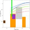 |
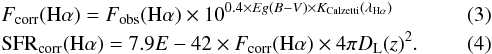
Fig. 6 Mass-metallicty relations as presented in Kewley & Ellison (2008) for log (M/M⊙) > 8.5. The color-coding is the same as in their Fig. 2. The cyan curve is obtained from the R23 calibration, blue, dashed black, and dashed red from a combination of R23 and [OIII]/[OII], solid black from a combination of line ratios, such as [OII], Hβ, [OIII], Hα, [NII], [SII], solid green from O3N2, solid yellow from N2, and solid red from the measurement of the electron temperature, using [OIII]4363, 4990, 5007. Shaded regions indicate the mass-metallicity area occupied by literature results within the error bars. Also shown is the Atek et al. (2011) source in brown at the lowest mass range, Finkelstein et al. (2011) upper limits in orange, Nakajima et al. (2012b) lower limit in green, and the range of objects from Xia et al. (2012)z > 1 in grey. The sources in our survey are characterized by 9 < log (M/M⊙) < 10, where the N2 and O3N2 agree with all the other calibrations within 0.4 dex. |
We chose recent literature estimations of metallicity of SFGs and LAEs to compare with in a meaningful way.
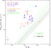 |
Fig. 7 SFRcorr(Hα) vs. stellar mass for LAEs and SFGs at z ≥ 2. Red and magenta colors indicate Lyα and Hα emitting galaxies, while blue indicate UV-continuum-selected SFGs without Lyα in emission. The blue star with cyan error bars represents BX16, which shows Lyα absorption. The SFR(Hα) upper limit is due to an upper limit in Hα flux, and lower limits are presented when it is not possible to estimate Eβ(B − V) from the rest-frame UV continuum slope for individual sources. The solid green line is the M∗ − SFR relation by Talia et al. (2012) for SFGs at z ≃2. The black line is the same relation for z ~ 2 SFGs in the GOODS survey (Daddi et al. 2007). Dashed green and black lines indicate the 1σ range of those relations. Measured values from Nakajima et al. (2012b) (green square), Finkelstein et al. (2011) (orange dots), Atek et al. (2011) (brown triangle), and Erb et al. (2010) (violet triangle) are also shown. |
Atek et al. (2011) used a direct method, measuring [OIII]4363 (dependent on electron temperature) versus [OIII]5007 to infer metallicity of line emitter sources at 0.35 < z < 2.3. This method is successfully applied to derive low-metallicities (7.1 < 12+log (O/H) < 8.3), because at higher metallicities [OIII]4363 becomes too weak to be measured. They discovered a very metal-poor source at z = 0.7 with 12+log (O/H) = 7.47 ± 0.11 and log (M∗/M⊙) < 8. Here, we took this source as an example of a very metal-poor line emitter. We also compared with Xia et al. (2012), which used the R23 (([OII]3727+[OIII]5007)/Hβ) method to estimate metallicity of SFGs with strong emission lines at z > 1.
In addition to them, we considered sources at z ≥ 2. The star-forming galaxy, named BX418, was found to have 12 +log (O/H) = 7.9 ± 0.2 (Erb et al. 2010, direct method). With EW(Lyα) = 54.0 ± 1.2 Å, it is one of the most metal-poor LAEs known at high redshift. Finkelstein et al. (2011) placed upper limits on metallicity for two LAEs at z = 2.3 and 2.5, using N2 and O3N2 from Pettini & Pagel (2004). They can be directly compared to our sources. Nakajima et al. (2012b) selected a sample of LAEs at z ~ 2.2 and were able to set a lower limit of 12 + log (O/H) ≥ 7.9 on the stacked object, using a combination of [OII]/Hβ and N2 calibrations. Nakajima et al. (2012a) used N2 from Maiolino et al. (2008) to infer 12+log (O/H) of individual sources, therefore their results can also be directly compared with ours.
We could apply neither R23 nor direct methods because in our MMIRS spectra we did not cover [OIII]4363 or [OII]3727.
In Fig. 6 we show the mass-metallicity (M∗ − Z) relations presented in (Kewley & Ellison 2008, their Fig. 2), with their same color coding. The shaded regions represent the ranges in stellar mass and metallicity for the literature results described above. Kewley & Ellison (2008) pointed out that their M∗ − Z relation, corresponding to the direct method, was characterized by high statistical uncertainty.
At the stellar mass of BX418 (log (M/M⊙) = 9.0), the discrepancy between the direct and N2 methods is less than 0.2 dex. In the range of masses covered by the Xia et al. (2012) sample, it is 0.3 dex between N2 and R23 estimators. In the range of masses probed by Nakajima et al. (2012b), it is less than 0.4 dex among all the calibrations. These discrepancies were within the error bars of the metallicity estimations of our sources. Therefore, our results could be compared with the literature ones just mentioned, reasonably without scaling to a common calibration (Sect. 6).
6. Discussion
We found the [OIII]4959, 5007 emission line doublet to be the strongest feature in MMIRS spectra of z ~ 2−3 sources. We detected the [OIII] doublet in 12 out of 13 galaxies, while we detected Hα in just 6 out of 10 z ~ 2 galaxies. This may be surprizing at first glance. However, for SFGs characterized by slightly sub-solar metallicity, [OIII]5007 is predicted and measured to be very strong (Schaerer & de Barros 2012). Kakazu et al. (2007) conducted a survey to search for ultra-strong emission line galaxies at 0 < z < 1. Their results showed that these galaxies contribute roughly 10% of the measured SFR density at that epoch. All the Hα emitters in their sample were metal-poor (Z < 0.45 Z⊙) galaxies, characterized by strong [OIII]4363, while [OII]3727 was found to be very weak compared to [OIII]5007. The higher-metallicity objects had, instead, stronger [OII]3727/[OIII]5007. They concluded that they were looking at galaxies different from local metal-poor dwarf galaxies with larger [OIII]5007/[OII]3727 flux ratio and more mass. This suggested an early chemical enrichment phase in galaxies which are still growing.
Also, in our spectra the sky background continuum can be 3 times higher at 22 000 Å than at 16 000 Å, and we measured an average fractional background error at 22 000 Å twice the one at 16 000 Å. In Figs. 4 and 5 we presented the spectra of the SFGs in our sample, separated into [OIII]doublet and Hα wavelength ranges.
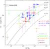 |
Fig. 8 Metallicity estimation versus stellar mass. The big magenta circle, red and blue stars correspond respectively to DB, LAEs and SFRs with EWrest−frame(Lyα) < 20 Å in our sample. Thin green upper limits and the green square are the data points from Nakajima et al. (2012a,b), small grey dots are Xia et al. (2012) values for z > 1 emitting galaxies. Black long-dashed, solid, dashed and dotted-dashed curves are the M∗ − Z relations from Maiolino et al. (2008) for the labeled redshifts. The horizontal solid line indicates solar metallicity (12+log (O/H) = 8.7). |
6.1. Star-forming galaxy evolutionary stage
Thanks to our spectroscopic results, we were able to place SFGs in the evolutionary sequence proposed by Noeske et al. (2007) (SFRcorr (Hα) versus stellar mass relation defined for log (M/M⊙) > 9.5 at z < 2). It was discovered that SFGs form a distinct sequence with a limited range of stellar masses. This “main sequence” moves as a whole to higher star formation rate as redshift increases. Therefore, galaxies of a given mass tended to present higher SFR at higher redshift; they were much more active on average in the past. One reason is the larger abundance of gas, depleted with time. For galaxies in the main sequence, the gradual accretion (as opposed to episodic and bursty events such as mergers) is the dominant process, and major mergers are not the dominant trigger of their star-formation activity and evolution. The outliers of the mass-SFR relation are galaxies with larger star-formation rate with respect to ordinary SFGs.
To completely fill this relation, we should be able to estimate SFR(Hα) for low mass (M∗ ≤ 109 M⊙) objects at z > 2. But the objects we detected in our spectroscopic survey tend to be bright in K band and therefore to be more massive than few ×109 M⊙. Ga2007 had first showed that z ≃ 3.1 LAEs are, typically, 109 M⊙ galaxies in their active phases of star formation and one of the highest specific SFR objects at that redshift. This is in favor of the idea that LAEs were still building stellar mass. If dust is an indication of a more evolved galaxy population and it is one of the reasons why Lyα photons cannot escape a galaxy ISM, we expect LAE to be characterized by lower mass and higher specific star formation rate. Nilsson et al. (2009) found that z ~ 2 LAEs instead presented a more massive (log (M/M⊙) ~ 9.5) sub-sample.
In Fig. 7 SFRcorr (Hα) is plotted versus stellar mass for SFGs at z ~ 2−3. Small symbols correspond to the literature data we chose for comparison, as described in the previous section. The lines (solid) with associated scatter (dashed) represent the correlation derived for z ~ 2 SFGs in the GOODS field by Daddi et al. (2007) and from GMASS (Galaxy Mass Assembly ultra-deep Spectroscopic Survey) by Talia et al. (2012). Our LAE and SFG data points tend to be characterized by higher SFR than typical z ~ 2 SFGs. Atek et al. (2011) observed that metal-poor galaxies at z ~ 1−2 are located towards the upper left corner of Daddi’s correlation, indicating that they are experiencing strong metal-poor burst episodes of star formation. The metal-poor source from Erb et al. (2010), the sources from Nakajima et al. (2012b), and the lowest mass LAE from Finkelstein et al. (2011) are also located in the same region.
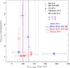 |
Fig. 9 F(Lyα)/F([OIII]5007) ratio versus the velocity offset between the same emission line central wavelengths. We present LAEs at z ≃ 2 in blue and at z ≃ 3 in red. The red asterisk is for LBG11. Data from McLinden et al. (2011) and (Finkelstein et al. 2011, updated by Chonis et al. priv. comm.) are shown as circles, from Erb et al. (2010) as triangle. The vertical lines represent the ranges of ΔvLyα − LIS by Shapley et al. (2003) (dashed) at z ~ 3, Berry et al. (2012) (solid) at z ~ 2 and 3, roughly divided by 3 to be compared with ΔvLyα − [OIII] 5007 (see text), and Steidel et al. (2010) (dotted). |
In Fig. 8 we show metallicity versus stellar mass for our and the literature sources we chose for comparison.
The sources detected so far in our survey are confirmed to be active star-forming, characterized by metallicity of the order of 0.3 < Z/Z⊙ < 1.2 (12 + log (O/H) ~ 8.2−8.8). As explained in Sect. 5.2.3, it is meaningful to compare our results with the ones presented in the figure. The black curves are the mass-metallicity relations from Maiolino et al. (2008), which used spectroscopic data from AMAZE (Assessing the Mass-Abundance redshift[-Z] Evolution). They estimated stellar masses assuming a Salpeter IMF, like in our SED fitting, and calculated the best fit parameters for the relation at z = 0.07 (dotted-dashed), z = 0.7 (dashed), z = 2.2 (solid, calibrated following Erb et al. (2006) observations), and z = 3.5 (long dashed). They showed evolution in the mass-metallicity relation stronger at lower stellar masses. Our six star-forming galaxy metallicity estimations are roughly consistent with Maiolino et al. (2008)M∗ − Z relation at z = 1−2. The Finkelstein et al. (2011) source with stellar mass bigger than 1010 M⊙ results in a very metal-poor object.
Our UV-bright LAEs do not seem to be the most metal-poor objects at this redshift, even if for a couple of them we just set upper limits. This could suggest an early chemical enrichment during the growth phase of individual z ~ 2−3 Lyα emitting galaxies (Kakazu et al. 2007). The Erb et al. and Atek et al. very metal-poor objects present values even lower than the lower limit inferred by Nakajima et al. (2012b) for z ~ 2.2 emitters.
The existence of a correlation between stellar mass and metallicity reflects the fundamental role that galaxy mass plays in galactic chemical evolution. It can mean that low-mass galaxies could be already experiencing a chemical enrichment phase. Also, galactic winds could be responsible in removing metals from galaxies (Tremonti et al. 2004; Rodrigues et al. 2012). This hypothesis could explain the metallicity lower than 7.9 obtained by Finkelstein et al. (2011) for a rare metal-poor source at that stellar mass. Tremonti et al. (2004) also noted that in large galaxies with deep potential wells, star formation activity and supernova explosions are not effective in pushing material in the form of an outflow. Inflows of metal-poor gas could either dilute the gas, reducing its metallicity, or turn on new star-formation episodes which would again metal-enrich the ISM. In addition to this, Mannucci et al. (2010) showed that the mass-metallicity relation, observed in the local and high-z Universe, may be due to a more general relation between stellar mass, metallicity and SFR. Based on their results, z ~ 2.5 SFGs with log (M∗/M⊙) = 9.7 are characterized by 12+log (O/H) of the order of 8.5−8.6, for star formation rates of about 30 M⊙ yr-1. For the same stellar mass and metallicity, the LAEs considered here could present even higher SFR. This can be an indication that different mechanisms could dominate in this kind of galaxies. We investigate the outflow hypothesis in the next sub-section and how it is related to the Lyα luminosity.
We are not yet able to derive conclusions about either M∗ − Z or M∗ − SFR relations of LAEs and SFGs at the same redshift. On-coming spectroscopic data are needed to support the hypothesis that z ~ 2 LAE could be younger but more metal-rich than z ~ 3 LAEs, as found by Acquaviva et al. (2012).
6.2. Lyα emitter ISM properties
From the MUSYC (FORS, VIMOS, and IMACS; see Berry et al. 2012) and GOODS-VIMOS spectroscopic surveys, we were able to measure Lyα fluxes (Fig. 9) for 2 LAEs at z ~ 2, 1 SF galaxy with Lyα in absorption, 2 LAEs at z ~ 3, and 1 LBG. GOODS 1D spectra were generated through an optimal extraction by following the slit profile measured in each slit. This minimized the slit losses for individual objects. Also, the GOODS team restricted the observations to airmass equal to 1.1, to minimize the loss of light due to atmospheric refractions (Popesso et al. 2009; Balestra et al. 2010).
The Lyα/Hα flux ratio is generally investigated to study the ISM nature (Hayes et al. 2010a; Finkelstein et al. 2011). In fact the presence of dust (to which the Balmer decrement is also sensitive) can significantly reduce the escape of Lyα versus Hα photons. For BX1 we calculated an escape fraction of Lyα photons of about 30% and for BX10 a lower limit of 7% due to F(Lyα)/F(Hα) ≥ 0.6. Finkelstein et al. (2011) calculated a ratio close to 7. First of all, they were observing two LAEs brighter in Lyα than our originally continuum-selected galaxies. Also, besides the big uncertainty and the low statistics, we could be observing individual LAEs with a higher dust amount than theirs. But they calculated E(B − V) = 0.20 ± 0.15 and E(B − V) < 0.13 from the Balmer decrement for their two objects. We estimated E(B − V) = 0.12 ± 0.02 (E(B − V) < 0.54) for BX1 and E(B − V) = 0.12 ± 0.02 for BX10 from fitting the UV β slope (Balmer decrement), which are consistent with theirs. Therefore, in addition to dust reddening, other ingredients of LAE ISM need to be considered to completely understand their properties, such as gas phase metallicity and kinematics.
For most emission line objects, the Lyα/[OIII]5007 flux ratio was calculated with high significance (S/N ≥ 3). This ratio is affected by gas phase metallicity, kinematics, and Lyα radiative transfer in the LAE ISM, related to the neutral Hydrogen content. Because metallicity could be a key ingredient which regulates Lyα photon escape, we note that Lyα/[OIII]5007, in addition to the Lyα/Hα or together with SED fitting, can be investigated to improve the understanding of star-forming galaxy ISM (temperature, metal abundances, geometry, kinematics). We noted a tentative trend between Lyα and [OIII]5007 emission lines, which could be related to the M∗ − Z relation. High statistics are needed to disentangle Lyα/[OIII]5007 dependence on metallicity and dust content.
We noted that SFGs at z ~ 2−3 show F(Lyα)/F([OIII]5007) ratio between 0 and 1, with z ~ 2 LAEs showing a ratio closer to 1 (Fig. 9). In addition to the flux uncertainty reported in Table 4, the uncertainties described in Sect. 4.1 are included in the [OIII] flux error budget. We used the public version of GalMC code (Acquaviva et al. 2011), which makes use of Anders & Fritse (2003) line ratios, to predict Lyα/[OIII]5007 ratios of typical SFGs at different values of galaxy age and metallicity (Z). Assuming an age of 108 yr, for 0.02 < Z/Z⊙ < 2.0, Lyα/[OIII]5007 can be between 5 and 8, assuming case B recombination and no dust. For E(B − V) = 0.1 it becomes 2.5 < Lyα/[OIII]5007 < 4.0 and for E(B − V) = 0.3 we calculated Lyα/[OIII]5007 < 1.0, assuming the Calzetti law. Also, in the absence of dust [OIII]5007/Hβ ~ 4 and [OIII]5007/Hα ~ 1.4. Therefore, a Lyα/[OIII]5007 ≤ 1.0 could be explained either with E(B − V) ~ 0.3, consistent with the SED fitting results, or involving radiative transfer effects, which preferentially absorb Lyα with respect to Hα and [OIII] photons. However, the referred Finkelstein’s LAEs present stronger Lyα emission with respect to [OIII] than ours and significantly lower metallicity.
It was proposed (Kunth et al. 1998; Heckman et al. 2001; Dijkstra et al. 2011, as examples) that galaxy outflows, driven by star formation activity, are able to red-shift the central wavelength of the Lyα photon λ-distribution. This way they appear invisible to neutral Hydrogen and can escape. To investigate the dependence of Lyα/[OIII] on kinematics we measured Lyα-[OIII] velocity offsets (Sect. 5.2.2).
Using stacked rest-frame UV spectra of a few LAEs in our sample, Berry et al. (2012) measured velocity offsets of about 600 km s-1 between Lyα and low-ionization absorption lines (LIS). As low-ionization absorption lines are thought to be tracing the neutral gas, this offset is thought to be produced because out-flowing neutral gas allows only the red side of Lyα line photons to escape, making it appear redshifted with respect to the systemic velocity. Here we estimated expansion velocities of possible outflows calculating velocity offsets between the central wavelength of Lyα with respect to that of metal lines at the systemic redshift.
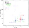 |
Fig. 10 Velocity offset between Lyα central wavelength and systemic redshift versus stellar mass. The color coding is as in Fig. 9. Green squares are from Hashimoto et al. (2013) for the sample of z ~ 2.2 LAEs, also studied in Nakajima et al. (2012a). The stellar masses of our sources are estimates from stacked SED fitting as explained in Sect. 5.2.1. |
In Fig. 9 we present the F(Lyα)/F([OIII]5007) ratio versus ΔvLyα − [OIII] 5007. In the figure we do not show the value of − 897.8 ± 257.0 km s-1, calculated for the SFG with Lyα in absorption (BX16). BX10 is characterized by 749.9 ± 188.3 km s-1 and the highest uncertainty in [OIII] central wavelength (18 095.5 ± 11.6 Å). In fact this emission line is on top of sky line residuals (Fig. 4), which affect the line integrated flux and central wavelength. However, we can not exclude it being a high-velocity-offset source. For the other three LAEs at z ~ 2−3 (star symbols), the offsets are 70−270 km s-1. These values are consistent with previous estimations from McLinden et al. (2011) and (Finkelstein et al. 2011; updated by Chonis et al., priv. comm.). For LBG11, we estimated ΔvLyα − [OIII] 5007 = 344.5 ± 107.0 km s-1, which is consistent with the value estimated by McLinden et al. (2011) for their strongest [OIII]5007 emission line LAE (F([OIII]5007) = (35.48 ± 1.15)E-17 erg s-1 cm-2) at similar redshift. The velocities we calculated here are also consistent with expansion velocities, Vexp = 100−300 km s-1, measured by Verhamme et al. (2008) for a sample of 11 LBGs. Instead, Steidel et al. (2010) estimated stronger velocity offsets of 445 ± 27 km s-1 for a sample of Hα emitters at z = 2.3. Their range of Vexp within 1σ is plotted as a rectangular region delimited by dotted lines.
While the outflow velocity, Vexp, is best estimated from the velocity difference between LIS, which trace the out-flowing material, and systemic redshift emission lines, ΔvLyα − [OIII] 5007 can give upper limits for commonly assumed geometries. In Berry et al. (2012) and Shapley et al. (2003), they estimated offsets between LIS absorption lines and Lyα, which could be up to three ×Vexp. It was shown in Verhamme et al. (2008) that for an expanding shell model ΔvLyα − LIS can be 3 (2) times of the expansion velocity, depending on the HI column density, NHI ≥ (< )1020/cm2. The situation can change for different geometries. In the figure the range of Vexp values from Shapley et al. (2003) is presented as the rectangle delimited by the red dashed lines, rescaled to be compared to our ΔvLyα − [OIII] 5007. The range of Vexp values from Berry et al. (2012) at z = 2 and z = 3 is also rescaled and it corresponds to the rectangle delimited by solid lines.
We fitted Lyα line profiles with single symmetrical Gaussian curves. The asymmetry of Lyα profile of LAEs at z ≃ 3.1 was quantified by McLinden et al. (2011) as the σGauss of the red peak divided by the σGauss of the blue peak (a). One of their two sources showed significant asymmetry in the Lyα line profile, a = 2.1 ± 0.2 (a = 1.0 ± 0.1 for the other source). They used the Hectospec multi-fiber spectrograph at the 6.5 m MMT observatory, with an instrument resolution of ~6 Å. We performed a test to estimate the centroid shift due to the symmetric versus asymmetric profile fit. A good fit to the data can be obtained with a symmetric profile and a central wavelength shift of about 1 Å in the rest frame. It implies a velocity offset of 60−80 km s-1 for LAEs at z ~ 3−2, which is within the error bars of our measurements.
We do not see any significant difference between redshift 2 and 3, but the statistics are still too low to derive strong conclusions. However, combining Figs. 8 and 9 we can observe that lower dust, lower metallicity, bright Lyα flux sources, such as the two LAEs studied by Finkelstein et al. (2011), tend to be characterized by velocity outflows similar to those of our sources. The rare metal-poor object by Finkelstein et al. (2011) could host an episode of chemical enrichment of pristine gas, also characterized by a low amount of dust. The sources in our survey could be galaxies in more evolved stages, but with hundred km s-1 outflows as channels for Lyα photon escape.
We are also interested in understanding how galaxy physical properties can relate to outflow expansion velocities. In Fig. 10 we plot ΔvLyα − [OIII] 5007 versus stellar mass for our survey of z ~ 2−3 SFGs and recent results described in the literature. The squares correspond to Hashimoto et al. (2013), who fitted individual galaxy SEDs to obtain stellar mass and used the MMIRS and Keck/NIRSPEC instrument to measure ΔvLyα − [OIII] 5007, ΔvLyα − Hα, and to infer Lyα velocity offsets. A weak trend of velocity offset with stellar mass can be seen, but individual cases of very high expansion velocity and log (M∗/M⊙) ~ 9.0 need to be investigated in more detail. This trend could be explained considering that low mass galaxies are still in the process of building up their mass and have a weak gravitational potential to support strong outflows (Heckman et al. 2001; Orsi et al. 2012). In this scenario log (M∗/M⊙) = 10 SFGs, like LBGs, could show higher velocity outflow. LBG11, for example, shows one of the highest Vexp of our sample. However, massive galaxies can be characterized by high HI column density (NHI ~ 1020/cm2), which would completely remove the Lyα line blue peak and would leave a Lyα emission line profile either asymmetric or double-peaked with the red side stronger than the blue one (Verhamme et al. 2008; Orsi et al. 2012). This would produce a big ΔvLyα − [OIII] 5007, without the need of strong Vexp. Multiple scattering can produce multiple peaks in the wings of the double-peaked profile (Kulas et al. 2012).
Additional investigation of Lyα line profile needs to be carried out to disentangle these hypotheses.
7. Summary and conclusions
In this paper we presented new spectroscopy of SFGs at z ~ 2−3 covered by MUSYC, probing nebular emission. The original aim was to detect [OIII] and Hα emission lines in SFGs to better understand their ISM properties (Table 5) and to relate them to Lyα emission line strength and profile, where observed. Details on MMIRS performance are presented in the Appendix. In Figs. 2, 4, 5 we showed the extracted and fitted 1D spectra for all the sources in our survey. In Tables 4−6 we presented measured line fluxes, flux ratios and galaxy physical properties. We list here the main conclusions of our NIR survey.
-
1)
We developed a reduction pipeline, which makes useof COSMOS software. We found COSMOS plusan ABBA source offset procedure successful in reducing MMIRS data (Sect. 3 and details in the Appendix A). We tested MMIRS behavior using high signal-to-noise spectra of AGNs in our masks.
-
2)
Through MMIRS spectra, we could confirm seven redshifts obtained via rest-frame UV spectra and determine seven(three) new redshifts of SFGs (AGNs).
-
3)
We estimated optical emission line intensity and line ratios for 13 SFGs, 6 of which were previously selected as either Lyα and/or Hα emitters. Two additional SFGs were discovered to be LAEs in GOODS public survey spectra. We found the [OIII]5007 emission line to be the most prominent one in our z ~ 2−3 galaxy spectra, which are all characterized by R ≤ 25.5.
-
4)
We adopted either rest-frame UV β slope or E(B − V)SED for reddening correction. We took advantage of the SED fitting results from Gu2011, Lai et al. (2008) and Hayes et al. (2010a) to estimate the stellar mass of the galaxies in our sample. In the M∗ − SFR(Hα) plane (Fig. 7), the SFGs in our sample were located towards the upper left corner of the correlation found for z ~ 2 SFGs by Daddi et al. (2007) and Talia et al. (2012). At fixed stellar mass, they presented larger SFR than typical SFGs. This implies that they are experiencing active bursts of star formation, which are building up their mass. One possibility can be the star-formation episodes implied by mergers (Noeske et al. 2007). As observed by Atek et al. (2011), low-metallicity sources occupy the same locus of the M∗ − SFR(Hα) plane. We estimated metallicity from Nagao (2006) and Maiolino (2008) [OIII]5007/Hβ, [OIII]5007/[NII]6584, and [NII]6584/Hα calibration. We chose a few metal-poor sources from the literature to compare our metallicity estimations and demonstrated it is meaningful to compare them. Due to weak Hβ and [NII] emission lines, we could estimate metallicity for two SFGs (one of which is selected to be Hα emitter) and set limits for another four. At 9 < log (M∗/M⊙) < 10 our sources have metallicity consistent with 12 + log (O/H) ~ 8.2−8.8. The two LAEs studied by Finkelstein et al. (2011) were significantly brighter in Lyα (3−6 times in the integrated line flux, Fig. 9), showed significantly lower metallicity, and had average lower SFRcorr(Hα) than ours. In the M∗ − Z plane, our sources agreed with the relations found by Maiolino et al. (2008) for z ≤ 2.2 galaxies. The sources detected so far in our survey are confirmed to be actively star-forming, characterized by metallicity of the order of 0.3 < Z/Z⊙ < 1.2. However, we are not yet able to derive strong conclusions about the connection between M∗ − Z and M∗ − SFR relations of LAEs and SFGs at the same redshift.
-
5)
We were able to study nebular emission from four LAEs, one SFG with Lyα in absorption, and one LBG with EWobs−frame(Lyα) = 34 Å (EWrest−frame(Lyα) ~ 2 Å). For high-redshift galaxies with both rest-UV and rest-frame optical spectroscopy, our observations indicate that the two emission lines with highest signal-to-noise will often be Lyα and [OIII]5007. For many dim objects, these will be the only lines detected. Hence, we find empirical motivation to form and study the Lyα/[OIII] flux ratio and to attempt to calibrate it both empirically and theoretically. This ratio is far from ideal as a physical tracer, being sensitive to a combination of metallicity, ionization, and Lyα radiative transfer in the ISM, and it will be challenging to model. But given the arrival of a generation of multi-object NIR spectrographs and the difficulty of detecting Hα for significant redshift ranges of interest, the Lyα/[OIII]5007 ratio is worthy of investigation.
Consistent with previous estimations ΔvLyα − [OIII] 5007 was positive, indicating the presence of outflows. We found that LAEs are characterized by Vexp ~ 70−270 km s-1, in agreement with Berry et al. (2012). However, the scattering of Lyα photons due to neutral Hydrogen atom, could mask the exact value of the outflow velocity. It was proposed by Tremonti et al. (2004) that outflows could remove metals together with neutral Hydrogen. Therefore, high-stellar-mass galaxies could have experienced outflow phenomena in the past and now show lower metallicity. The outflow phenomena could still be going on. However, our sources present just slightly sub-Z⊙. In Fig. 10 we showed velocity offset versus stellar mass. There is a weak trend for which higher mass SFGs could be characterized by higher velocity outflow. However, massive SFGs tend to be characterized by NHI ~ 1020/cm2, which could produce a strongly red-shifted red Lyα peak without the need for strong Vexp.
The MMIRS spectrograph can be successfully used to study nebular emission of bright SFGs at z ~ 2−3, but a larger sample of galaxies is needed to derive strong conclusions.
Online material
Emission line fluxes for all the sources.
Galaxy metallicity.
Galaxy properties.
Appendix A: MMIRS data reduction and performance
Appendix A.1: Reduction procedure
The raw mask frames, output of MMIRS, are multi-extension files. The 3nd to Nth extensions are characterized by individual exposure times equal to t_ramp up to t_total−t_ramp, where t_ramp is the ramp-up time and t_total is the total exposure time of the frame. The read-out is done using a ramp-up procedure, optimized to avoid saturation. It is made every t_ramp seconds, t_total/t_ramp times. The 1st extension in the multi-extension MMIRS frame contains the total exposure time, while the 2nd contains the zero-level counts.
Dark frames are obtained in the morning for every kind of exposure taken during the previous night and in series of 5 (ramped-up multi-extension darks should be subtracted from the ramped-up science frames). We average combined multi-extension dark frames, using IRAF mscred.combine task.
The following step of our reduction pipeline is collapsing all of the information enclosed in the multi-extension files. We used mmfixen code. The information contained in the N extensions are combined, saturated pixels are filled and cosmic rays are removed. The output is a new multi-extension file, in which the 1st extension is the science frame normalized to counts/sec, the 2nd, 3rd and 4th contain statistical information about the image and the fitting process.
We ran mmfixen code for all the ramped-up science frames and then we extracted their 1st extensions. In the case of t_total<t_ramp we just subtracted the zero-level counts (2nd extension) to the 1st extension. It happened for the majority of flat frames and for standard stars. We then normalized flat frames, slit by slit, using IRAF twodspec.longslit.response task and we divided science and standard frames by the normalized flat.
COSMOS software was used to generate the wavelength map needed for wavelength calibration. We first obtained a rough wavelength map using the calibration lamp. The spectra of an Argon9 lamp are obtained through each slit of a mask. Lamp emission line pixels were related to known wavelengths using COSMOS align-mask and adjust-offset codes. An improved wavelength solution and spectral map were calculated using a few isolated sky lines in science frames. 10 We then ran COSMOS adjust-map to obtain the final solution, which contains the best wavelength map for all the mask slits together and it is satisfied by the entire series of sky lines from ~14 000 to ~22 000 Å.
We applied an ABBA procedure to get rid of prominent sky lines. In our May, 2011 run, sky line variations and along individual lines were stronger. Therefore, we got a better sky subtraction in Nov frames. We had the case of the first night of May run in which SDSS mask frames were not ramped-up. We just dark-subtracted and flat-divided them and directly applied this ABBA procedure. We then removed cosmic rays using IRAF
xdimsum.xzap task to ABBA frames to eliminate cosmic rays, coming from A, and to the inverse of ABBA to eliminate cosmic rays, coming from B. We checked the alignment of the ABBA frames, looking at the continuum spectra of alignment stars (also slit stars in the case of May run) and combined all the aligned ABBA frames of the same mask.
We finally applied COSMOS extract-2dspec code to wavelength calibrate the completely reduced frame and divide it in individual-slit 2D spectra.
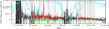 |
Fig. A.1 1D spectrum of z2LAE3 along the entire MMIRS coverage. The black (red) curve represents the raw (smoothed) spectrum. Grey vertical lines indicate the wavelength of the dominant sky emission lines. Cyan curve represents the atmospheric transmission at Las Campanas observatory. At λ ~ 14 000 and ~19 000 Å the transmission is very low. The green curve represents the background spectrum extracted far from the center of the slit where the source is positioned. Sky line residuals produce higher uncertainty. Telluric correction fixes the continuum shape but increases the uncertainty. Wavelength regions of high noise are not shown in the smoothed spectrum. |
Appendix A.2: Flux calibration
We used IRAF twodspec.apextract.apall task to extract 1D spectra. For standard stars we located the extraction aperture in a region of their continuum not affected by atmospheric absorption. For science spectra we chose the pixel position of the few prominent emission lines.
The three standard stars chosen at the observatory are telluric stars. Therefore they allowed to perform the correction for telluric features of science frames and also their flux calibration. Spectra coming from the same star, but obtained through different slits along a mask, cover different wavelength regions, depending on the position of the slit along the dispersion axis. They present comparable shapes in the common wavelength regions, but their relative intensity depends on the mask orientation and on the sky conditions, that can change with time. These variations are reflected in the science frames as well. So we average-combined all the 1D spectra of the same telluric stars of the run, taken at the same airmass of the science frames.
We extracted 1D spectra of the objects in the center of the slits as well as the ones of the background either on the upper or lower side of the slits to estimate background fluctuations, after sky emission line removal. In Fig. A.1 we show z2LAE3 raw(smoothed) spectrum in black(red) and the background spectrum in green. This background spectrum is a proxy of the noise spectrum of this object.
Appendix B: MMIRS 2D spectra and performance
As we could see in Table 2, z < 1.4 “low-z” galaxies and slit stars were located in MMIRS masks as a test of its performance. Figure B.1 shows 2D spectra of two slit stars in SDSS (upper) and EHDF-S (lower) masks. A star of KAB = 16.42 starts to show saturation in an MMIRS spectrum, while the continuum of a KAB = 17.81 star is clearly detected. Regions of strong atmospheric absorption are clearly seen, at ~14 000 Å (in the left side of the spectra), at ~19 000 Å (in the center-right side of the spectra). In these specific cases the slits were located at the same position along the dispersion axis of MMIRS mask. In Fig. B.2 we present the 2D spectra of 5 low-z galaxies obtained with SDSS mask. The top panel shows the source with the brightest KAB band mag of 17.65. The continuum appears well detected for sources with KAB ≤ 19.39.
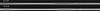 |
Fig. B.1 2D spectra of two slit stars in the SDSS and EHDF-S masks with KAB = 17.81 (up) and KAB = 16.42 (low), respectively. |
 |
Fig. B.2 2D spectra of the “low-z”, low-redshift galaxies obtained with SDSS mask. The spectra are aligned in wavelength. The top panel shows SDSS28 with the highest KAB band mag of 17.65. These sources spanned KAB band magnitudes from 17.65 (SDSS28), 19.39 (SDSS12) to 20.46. In the center of the stripes (~19 000 Å), the decrease in flux indicates the wavelength region of strong atmospheric absorption. We can also see regions of high Poisson noise due to sky emission lines. |
Acknowledgments
We are grateful for support from the following NSF grants:10-55919, 08-07570, 08-07885; from Basal-CATA PFB-06/2007 (HF, FEB, NP), CONICYT-Chile under grants FONDECYT 1101024 (FEB), ALMA-CONICYT 31100004 (FEB), and ANILLO ACT1101 (FEB), and Chandra X-ray Center grant SAO SP1-12007B (FEB); from CONICYT-Chile under grant FONDECYT 3100025, Comit Mixto ESO-Chile and FONDAP Center for Astrophysics 15010003 (HF); from Fondecyt Regular 1110327 (NP). We gratefully thank CNTAC for their generous support of our observing programs CHILE-2010B-0046 and CHILE-2011A-0002. We acknowledge Brian McLeod and Paul Martini for their strong help given during the reduction process of MMIRS data, Francesco di Mille and Vincent Suc for helping during the observations, and Anthony Gonzalez, Mike Berry, and Robin Ciardullo for useful comments that improved this paper. L.G. thanks Peter Kurczynski, Peter Laursen, Erik Zackrisson and Florent Duval for useful discussions.
References
- Acquaviva, V., Gawiser, E., & Guaita, L. 2011, ApJ, 737, 47 [NASA ADS] [CrossRef] [Google Scholar]
- Acquaviva, V., Vargas, C., Gawiser, E., & Guaita, L. 2012, ApJ, 751, L26 [NASA ADS] [CrossRef] [Google Scholar]
- Atek, H., Siana, B., Scarlata, C., et al. 2011, ApJ, 743, 121 [NASA ADS] [CrossRef] [Google Scholar]
- Baldwin, J. A., Phillips, M. M., & Terlevich, R. 1981, PASP, 93, 5 [NASA ADS] [CrossRef] [EDP Sciences] [Google Scholar]
- Balestra, I., Mainieri, V., Popesso, P., et al. 2010, A&A, 512, A12 [NASA ADS] [CrossRef] [EDP Sciences] [Google Scholar]
- Berry, M., Gawiser, E., Guaita, L., et al. 2012, ApJ, 749, 4 [NASA ADS] [CrossRef] [Google Scholar]
- Blanc, G. A., Lira, P., Barrientos, L. F., et al. 2008, ApJ, 681, 1099 [NASA ADS] [CrossRef] [Google Scholar]
- Bond, N. A., Gawiser, E., Guaita, L., et al. 2012, ApJ, 753, 95 [NASA ADS] [CrossRef] [Google Scholar]
- Calzetti, D., Armus, L., Bohlin, R. C., et al. 2000, ApJ, 533, 682 [NASA ADS] [CrossRef] [Google Scholar]
- Ciardullo, R., Gronwall, C., Wolf, C., et al. 2012, ApJ, 744, 110 [NASA ADS] [CrossRef] [Google Scholar]
- Cowie, L. L., & Hu, E. M. 1998, AJ, 115, 1319 [NASA ADS] [CrossRef] [Google Scholar]
- Daddi, E., Dickinson, M., Morrison, G., et al. 2007, ApJ, 670, 156 [NASA ADS] [CrossRef] [Google Scholar]
- Del Moro, A., Watson, M. G., Mateos, S., et al. 2009, A&A, 493, 445 [NASA ADS] [CrossRef] [EDP Sciences] [Google Scholar]
- Dijkstra, M., Mesinger, A., & Wyithe, J. S. B. 2011, MNRAS, 414, 2139 [NASA ADS] [CrossRef] [Google Scholar]
- Dunkley, J., Komatsu, E., Nolta, M. R., et al. 2009, ApJS, 180, 306 [NASA ADS] [CrossRef] [Google Scholar]
- Erb, D. K., Steidel, C. C., Shapley, A. E., et al. 2006, ApJ, 646, 107 [NASA ADS] [CrossRef] [Google Scholar]
- Erb, D. K., Pettini, M., Shapley, A. E., et al. 2010, ApJ, 719, 1168 [NASA ADS] [CrossRef] [Google Scholar]
- Finkelstein, S. L., Hill, G. J., Gebhardt, K., et al. 2011, ApJ, 729, 140 [NASA ADS] [CrossRef] [Google Scholar]
- Francke, H., Gawiser, E., Lira, P., et al. 2008, ApJ, 673, L13 [NASA ADS] [CrossRef] [Google Scholar]
- Gawiser, E., van Dokkum, P. G., Herrera, D., et al. 2006, ApJS, 162, 1 [NASA ADS] [CrossRef] [Google Scholar]
- Gawiser, E., Francke, H., Lai, K., et al. 2007, ApJ, 671, 278 [NASA ADS] [CrossRef] [Google Scholar]
- Gronwall, C., Ciardullo, R., Hickey, T., et al. 2007, ApJ, 667, 79 [NASA ADS] [CrossRef] [Google Scholar]
- Guaita, L., Gawiser, E., Padilla, N., et al. 2010, ApJ, 714, 255 [NASA ADS] [CrossRef] [Google Scholar]
- Guaita, L., Acquaviva, V., Padilla, N., et al. 2011, ApJ, 733, 114 [NASA ADS] [CrossRef] [Google Scholar]
- Hashimoto, T., Ouchi, M., Shimasaku, K., et al. 2013, ApJ, 765, 70 [NASA ADS] [CrossRef] [Google Scholar]
- Hatch, N. A., Kurk, J. D., Pentericci, L., et al. 2011, MNRAS, 415, 2993 [NASA ADS] [CrossRef] [Google Scholar]
- Hayashi, M., Kodama, T., Koyama, Y., Tadaki, K.-I., & Tanaka, I. 2011, MNRAS, 415, 2670 [NASA ADS] [CrossRef] [Google Scholar]
- Hayes, M., Östlin, G., Schaerer, D., et al. 2010a, Nature, 464, 562 [NASA ADS] [CrossRef] [PubMed] [Google Scholar]
- Hayes, M., Schaerer, D., & Östlin, G. 2010b, A&A, 509, L5 [NASA ADS] [CrossRef] [EDP Sciences] [Google Scholar]
- Heckman, T. M., Sembach, K. R., Meurer, G. R., et al. 2001, ApJ, 558, 56 [NASA ADS] [CrossRef] [Google Scholar]
- Hu, E. M., Cowie, L. L., Kakazu, Y., & Barger, A. J. 2009, ApJ, 698, 2014 [NASA ADS] [CrossRef] [Google Scholar]
- Kakazu, Y., Cowie, L. L., & Hu, E. M. 2007, ApJ, 668, 853 [NASA ADS] [CrossRef] [Google Scholar]
- Kennicutt, Jr., R. C. 1998, ARA&A, 36, 189 [Google Scholar]
- Kewley, L. J., & Ellison, S. L. 2008, ApJ, 681, 1183 [NASA ADS] [CrossRef] [Google Scholar]
- Kewley, L. J., Heisler, C. A., Dopita, M. A., & Lumsden, S. 2001, ApJS, 132, 37 [NASA ADS] [CrossRef] [Google Scholar]
- Kulas, K. R., Shapley, A. E., Kollmeier, J. A., et al. 2012, ApJ, 745, 33 [NASA ADS] [CrossRef] [Google Scholar]
- Kunth, D., Mas-Hesse, J. M., Terlevich, E., et al. 1998, A&A, 334, 11 [NASA ADS] [Google Scholar]
- Lai, K., Huang, J.-S., Fazio, G., et al. 2008, ApJ, 674, 70 [NASA ADS] [CrossRef] [Google Scholar]
- Lee, J. C., Ly, C., Spitler, L., et al. 2012, PASP, 124, 782 [NASA ADS] [CrossRef] [Google Scholar]
- Maiolino, R., Nagao, T., Grazian, A., et al. 2008, A&A, 488, 463 [NASA ADS] [CrossRef] [EDP Sciences] [Google Scholar]
- Mannucci, F., Cresci, G., Maiolino, R., Marconi, A., & Gnerucci, A. 2010, MNRAS, 408, 2115 [NASA ADS] [CrossRef] [Google Scholar]
- McLinden, E. M., Finkelstein, S. L., Rhoads, J. E., et al. 2011, ApJ, 730, 136 [NASA ADS] [CrossRef] [Google Scholar]
- Miller, J. S., & Mathews, W. G. 1972, ApJ, 172, 593 [NASA ADS] [CrossRef] [Google Scholar]
- Miller, N. A., Fomalont, E. B., Kellermann, K. I., et al. 2008, ApJS, 179, 114 [NASA ADS] [CrossRef] [Google Scholar]
- Nagao, T., Maiolino, R., & Marconi, A. 2006, A&A, 459, 85 [NASA ADS] [CrossRef] [EDP Sciences] [Google Scholar]
- Nakajima, K., Ouchi, M., Shimasaku, K., et al. 2012a, ApJ, submitted [arXiv:1208.3260] [Google Scholar]
- Nakajima, K., Ouchi, M., Shimasaku, K., et al. 2012b, ApJ, 745, 12 [NASA ADS] [CrossRef] [Google Scholar]
- Nilsson, K. K., Tapken, C., Møller, P., et al. 2009, A&A, 498, 13 [NASA ADS] [CrossRef] [EDP Sciences] [Google Scholar]
- Nilsson, K. K., Östlin, G., Møller, P., et al. 2011, A&A, 529, A9 [NASA ADS] [CrossRef] [EDP Sciences] [Google Scholar]
- Noeske, K. G., Faber, S. M., Weiner, B. J., et al. 2007, ApJ, 660, L47 [NASA ADS] [CrossRef] [Google Scholar]
- Ono, Y., Ouchi, M., Shimasaku, K., et al. 2010, MNRAS, 402, 1580 [NASA ADS] [CrossRef] [Google Scholar]
- Onodera, M., Daddi, E., Gobat, R., et al. 2010, ApJ, 715, L6 [NASA ADS] [CrossRef] [Google Scholar]
- Orsi, A., Lacey, C. G., & Baugh, C. M. 2012, MNRAS, 425, 87 [NASA ADS] [CrossRef] [Google Scholar]
- Osterbrock, D. E. 1989, S&T, 78, 491 [NASA ADS] [Google Scholar]
- Ouchi, M., Shimasaku, K., Akiyama, M., et al. 2008, ApJS, 176, 301 [NASA ADS] [CrossRef] [Google Scholar]
- Pentericci, L., Grazian, A., Fontana, A., et al. 2007, A&A, 471, 433 [NASA ADS] [CrossRef] [EDP Sciences] [Google Scholar]
- Pettini, M., & Pagel, B. E. J. 2004, MNRAS, 348, L59 [NASA ADS] [CrossRef] [Google Scholar]
- Popesso, P., Dickinson, M., Nonino, M., et al. 2009, A&A, 494, 443 [NASA ADS] [CrossRef] [EDP Sciences] [Google Scholar]
- Rhoads, J. E., Malhotra, S., Dey, A., et al. 2000, ApJ, 545, L85 [NASA ADS] [CrossRef] [Google Scholar]
- Rodrigues, M., Puech, M., Hammer, F., Rothberg, B., & Flores, H. 2012, MNRAS, 421, 2888 [NASA ADS] [CrossRef] [Google Scholar]
- Rousselot, P., Lidman, C., Cuby, J.-G., Moreels, G., & Monnet, G. 2000, A&A, 354, 1134 [NASA ADS] [Google Scholar]
- Schaerer, D., & de Barros, S. 2012, IAU Symp., 284, 20 [NASA ADS] [Google Scholar]
- Scholz, A., Geers, V., Jayawardhana, R., et al. 2009, ApJ, 702, 805 [NASA ADS] [CrossRef] [Google Scholar]
- Shapley, A. E., Steidel, C. C., Pettini, M., & Adelberger, K. L. 2003, ApJ, 588, 65 [NASA ADS] [CrossRef] [Google Scholar]
- Shim, H., Chary, R.-R., Dickinson, M., et al. 2011, ApJ, 738, 69 [NASA ADS] [CrossRef] [Google Scholar]
- Shimizu, I., & Umemura, M. 2010, MNRAS, 406, 913 [NASA ADS] [Google Scholar]
- Steidel, C. C., Erb, D. K., Shapley, A. E., et al. 2010, ApJ, 717, 289 [NASA ADS] [CrossRef] [Google Scholar]
- Storey, P. J., & Zeippen, C. J. 2000, MNRAS, 312, 813 [Google Scholar]
- Talia, M., Mignoli, M., Cimatti, A., et al. 2012, A&A, 539, A61 [NASA ADS] [CrossRef] [EDP Sciences] [Google Scholar]
- Tanaka, I., Breuck, C. D., Kurk, J. D., et al. 2011, PASJ, 63, 415 [NASA ADS] [Google Scholar]
- Thompson, D., Djorgovski, S., & Beckwith, S. V. W. 1994, AJ, 107, 1 [NASA ADS] [CrossRef] [Google Scholar]
- Tremonti, C. A., Heckman, T. M., Kauffmann, G., et al. 2004, ApJ, 613, 898 [NASA ADS] [CrossRef] [Google Scholar]
- van Dokkum, P. G., Kriek, M., Rodgers, B., Franx, M., & Puxley, P. 2005, ApJ, 622, L13 [NASA ADS] [CrossRef] [Google Scholar]
- Verhamme, A., Schaerer, D., & Maselli, A. 2006, A&A, 460, 397 [NASA ADS] [CrossRef] [EDP Sciences] [Google Scholar]
- Verhamme, A., Schaerer, D., Atek, H., & Tapken, C. 2008, A&A, 491, 89 [NASA ADS] [CrossRef] [EDP Sciences] [Google Scholar]
- Xia, L., Malhotra, S., Rhoads, J., et al. 2012, AJ, 144, 28 [NASA ADS] [CrossRef] [Google Scholar]
- Xue, Y. Q., Luo, B., Brandt, W. N., et al. 2011, ApJS, 195, 10 [NASA ADS] [CrossRef] [Google Scholar]
- Yoshikawa, T., Akiyama, M., Kajisawa, M., et al. 2010, ApJ, 718, 112 [NASA ADS] [CrossRef] [Google Scholar]
All Tables
All Figures
|
Fig. 1 2D spectra of AGNs detected in the 4 masks, all characterized by KAB > 20. The spectra are aligned in wavelength. Poisson noise due to sky emission line residuals can be seen as black vertical stripes. |
| In the text | |
|
Fig. 2 Observed 1D spectra of AGNs in grey and best fit in red. From the top AGN5, BzK25, AGN26, z2LAE3. Vertical dashed lines represent the wavelengths of sky line residuals. The blue curve is the sky spectrum by Rousselot et al. (2000), which indicates the relative intensity of the OH emission lines. It has been scaled according to the panel axis to be visible. [OIII] doublet (Hα) wavelength ranges are presented in the left (right) panels. |
| In the text | |
|
Fig. 3 Line ratio diagrams as presented in Kewley et al. (2001) (solid lines). The solid lines divide AGNs from Starburst galaxies. Symbols indicate AGNs found in our survey as explained in the text, the filled (open) squares are our (van Dokkum et al. 2005) ratio estimations for AGN5, the black triangle (pentagon) represents Bzk25 (AGN26), the red star z2LAE3. SFGs located in the region typical of Starbursts are presented for comparison: DB12 as a magenta circle, BX16 as a cyan star, and the two LAEs from Finkelstein et al. (2011) as orange dots. |
| In the text | |
|
Fig. 4 Observed-frame 1D spectra (black curve) of the sources showing either Lyα in emission or in absorption in rest-frame UV spectra. In red we show the best fit model spectra. From the top BX1, BX10, LAE27, z3LAE2, BX16, LBG11. The first, second and third panel columns represent Lyα (from MUSYC and GOODS-VIMOS surveys), [OIII]doublet and Hα wavelength ranges respectively. Dashed vertical lines indicate the wavelength of sky emission lines, which could leave residuals in the science spectra. Horizontal dashed blue lines indicate the continuum rms in the wavelength range where we did not see an expected emission line. As LAE27, z3LAE2, and LBG11 are at z ~ 3, Hα line would fall outside the MMIRS coverage. The rest-frame optical emission lines are unresolved. |
| In the text | |
|
Fig. 5 Observed 1D spectra (grey curves) of the SFGs detected in our survey, without spectroscopic rest-frame UV counterparts (DB8, DB12, DB22, z2LAE2, BX4, BX7, BX14). [OIII]doublet and Hα regions are shown. If only one of these is detected, red vertical dashed lines indicate the location of Hα ([OIII]5007) lines which would be implied by the detected-line redshift for DB8, DB22, z2LAE2 (BX4). Dashed grey vertical lines indicate the wavelength of sky emission lines, which could leave residuals in the science spectra. Horizontal dashed blue lines represent the continuum rms in the wavelength range where we did not see an expected emission line. |
| In the text | |
|
Fig. 6 Mass-metallicty relations as presented in Kewley & Ellison (2008) for log (M/M⊙) > 8.5. The color-coding is the same as in their Fig. 2. The cyan curve is obtained from the R23 calibration, blue, dashed black, and dashed red from a combination of R23 and [OIII]/[OII], solid black from a combination of line ratios, such as [OII], Hβ, [OIII], Hα, [NII], [SII], solid green from O3N2, solid yellow from N2, and solid red from the measurement of the electron temperature, using [OIII]4363, 4990, 5007. Shaded regions indicate the mass-metallicity area occupied by literature results within the error bars. Also shown is the Atek et al. (2011) source in brown at the lowest mass range, Finkelstein et al. (2011) upper limits in orange, Nakajima et al. (2012b) lower limit in green, and the range of objects from Xia et al. (2012)z > 1 in grey. The sources in our survey are characterized by 9 < log (M/M⊙) < 10, where the N2 and O3N2 agree with all the other calibrations within 0.4 dex. |
| In the text | |
|
Fig. 7 SFRcorr(Hα) vs. stellar mass for LAEs and SFGs at z ≥ 2. Red and magenta colors indicate Lyα and Hα emitting galaxies, while blue indicate UV-continuum-selected SFGs without Lyα in emission. The blue star with cyan error bars represents BX16, which shows Lyα absorption. The SFR(Hα) upper limit is due to an upper limit in Hα flux, and lower limits are presented when it is not possible to estimate Eβ(B − V) from the rest-frame UV continuum slope for individual sources. The solid green line is the M∗ − SFR relation by Talia et al. (2012) for SFGs at z ≃2. The black line is the same relation for z ~ 2 SFGs in the GOODS survey (Daddi et al. 2007). Dashed green and black lines indicate the 1σ range of those relations. Measured values from Nakajima et al. (2012b) (green square), Finkelstein et al. (2011) (orange dots), Atek et al. (2011) (brown triangle), and Erb et al. (2010) (violet triangle) are also shown. |
| In the text | |
|
Fig. 8 Metallicity estimation versus stellar mass. The big magenta circle, red and blue stars correspond respectively to DB, LAEs and SFRs with EWrest−frame(Lyα) < 20 Å in our sample. Thin green upper limits and the green square are the data points from Nakajima et al. (2012a,b), small grey dots are Xia et al. (2012) values for z > 1 emitting galaxies. Black long-dashed, solid, dashed and dotted-dashed curves are the M∗ − Z relations from Maiolino et al. (2008) for the labeled redshifts. The horizontal solid line indicates solar metallicity (12+log (O/H) = 8.7). |
| In the text | |
|
Fig. 9 F(Lyα)/F([OIII]5007) ratio versus the velocity offset between the same emission line central wavelengths. We present LAEs at z ≃ 2 in blue and at z ≃ 3 in red. The red asterisk is for LBG11. Data from McLinden et al. (2011) and (Finkelstein et al. 2011, updated by Chonis et al. priv. comm.) are shown as circles, from Erb et al. (2010) as triangle. The vertical lines represent the ranges of ΔvLyα − LIS by Shapley et al. (2003) (dashed) at z ~ 3, Berry et al. (2012) (solid) at z ~ 2 and 3, roughly divided by 3 to be compared with ΔvLyα − [OIII] 5007 (see text), and Steidel et al. (2010) (dotted). |
| In the text | |
|
Fig. 10 Velocity offset between Lyα central wavelength and systemic redshift versus stellar mass. The color coding is as in Fig. 9. Green squares are from Hashimoto et al. (2013) for the sample of z ~ 2.2 LAEs, also studied in Nakajima et al. (2012a). The stellar masses of our sources are estimates from stacked SED fitting as explained in Sect. 5.2.1. |
| In the text | |
|
Fig. A.1 1D spectrum of z2LAE3 along the entire MMIRS coverage. The black (red) curve represents the raw (smoothed) spectrum. Grey vertical lines indicate the wavelength of the dominant sky emission lines. Cyan curve represents the atmospheric transmission at Las Campanas observatory. At λ ~ 14 000 and ~19 000 Å the transmission is very low. The green curve represents the background spectrum extracted far from the center of the slit where the source is positioned. Sky line residuals produce higher uncertainty. Telluric correction fixes the continuum shape but increases the uncertainty. Wavelength regions of high noise are not shown in the smoothed spectrum. |
| In the text | |
|
Fig. B.1 2D spectra of two slit stars in the SDSS and EHDF-S masks with KAB = 17.81 (up) and KAB = 16.42 (low), respectively. |
| In the text | |
|
Fig. B.2 2D spectra of the “low-z”, low-redshift galaxies obtained with SDSS mask. The spectra are aligned in wavelength. The top panel shows SDSS28 with the highest KAB band mag of 17.65. These sources spanned KAB band magnitudes from 17.65 (SDSS28), 19.39 (SDSS12) to 20.46. In the center of the stripes (~19 000 Å), the decrease in flux indicates the wavelength region of strong atmospheric absorption. We can also see regions of high Poisson noise due to sky emission lines. |
| In the text | |
Current usage metrics show cumulative count of Article Views (full-text article views including HTML views, PDF and ePub downloads, according to the available data) and Abstracts Views on Vision4Press platform.
Data correspond to usage on the plateform after 2015. The current usage metrics is available 48-96 hours after online publication and is updated daily on week days.
Initial download of the metrics may take a while.