| Issue |
A&A
Volume 672, April 2023
|
|
|---|---|---|
| Article Number | A11 | |
| Number of page(s) | 28 | |
| Section | Extragalactic astronomy | |
| DOI | https://doi.org/10.1051/0004-6361/202245167 | |
| Published online | 23 March 2023 | |
Lyman continuum leaker candidates among highly ionised, low-redshift dwarf galaxies selected from He II
1
Ruhr University Bochum, Faculty of Physics and Astronomy, Astronomical Institute (AIRUB), Universitätsstrasse 150, 44801 Bochum, Germany
e-mail: This email address is being protected from spambots. You need JavaScript enabled to view it.
2
Ruhr Astroparticle and Plasma Physics Center (RAPP Center), Ruhr-Universität Bochum, 44780 Bochum, Germany
3
Ruhr University Bochum, Research Department, Plasmas with Complex Interactions, 44780 Bochum, Germany
Received:
7
October
2022
Accepted:
31
January
2023
Abstract
Context. Contemporary research suggests that the reionisation of the intergalactic medium (IGM) in the early Universe was predominantly realised by star-forming (proto-)galaxies (SFGs). Due to observational constraints, our knowledge on the origins of sufficient amounts of ionising Lyman continuum (LyC) photons and the mechanisms facilitating their transport into the IGM remains sparse. Recent efforts have thus focussed on the study of local analogues to these high-redshift objects.
Aims. We aim to acquire a set of very low-redshift SFGs that exhibit signs of a hard radiation field being present. A subsequent analysis of their emission line properties is intended to shed light on how the conditions prevalent in these objects compare to those predicted to be present in early SFGs that are thought to be LyC emitters (LCEs).
Methods. We used archival spectroscopic SDSS DR12 data to select a sample of low-redshift He II 4686 emitters and restricted it to a set of SFGs with an emission line diagnostic sensitive to the presence of an active galactic nucleus, which serves as our only selection criterion. We performed a population spectral synthesis with FADO to reconstruct these galaxies’ star-formation histories (SFHs). Utilising the spectroscopic information at hand, we constrained the predominant ionisation mechanisms in these galaxies and inferred information on interstellar medium (ISM) conditions relevant for the escape of LyC radiation.
Results. Our final sample consists of eighteen ionised, metal-poor galaxies (IMPs). These low-mass (6.2 ≤ log(M⋆/M⊙) ≤ 8.8), low-metallicity (7.54 ≤ log(O/H) + 12 ≤ 8.13) dwarf galaxies appear to be predominantly ionised by stellar sources. We find large [OIII] 5007/[OII] 3727 ratios and [SII] 6717,6731/Hα deficiencies, which provide strong indications for these galaxies to be LCEs. At least 40% of these objects are candidates for featuring cosmologically significant LyC escape fractions ≳10%. The IMPs’ SFHs exhibit strong similarities and almost all galaxies appear to contain an old (> 1 Gyr) stellar component, while also harbouring a young, two-stage (∼10 Myr and < 1 Myr) starburst, which we speculate might be related to LyC escape.
Conclusions. The properties of the compact emission line galaxies presented here align well with those observed in many local LCEs. In fact, our sample may prove as an extension to the rather small catalogue of local LCEs, as the extreme ISM conditions we find are assumed to facilitate LyC leakage. Notably, all of our eighteen candidates are significantly closer (z < 0.1) than most established LCEs. If the inferred LyC photon loss is genuine, this demonstrates that selecting SFGs from He II 4686 is a powerful selection criterion in the search for LCEs.
Key words: galaxies: abundances / galaxies: dwarf / galaxies: fundamental parameters / galaxies: ISM / galaxies: starburst / dark ages, reionization, first stars
© The Authors 2023
 Open Access article, published by EDP Sciences, under the terms of the Creative Commons Attribution License (https://creativecommons.org/licenses/by/4.0), which permits unrestricted use, distribution, and reproduction in any medium, provided the original work is properly cited.
This article is published in open access under the Subscribe to Open model. This email address is being protected from spambots. You need JavaScript enabled to view it. to support open access publication.
1. Introduction
About 12.8 Gyr ago, at a redshift of z ∼ 6, the last major phase transition of our Universe’s intergalactic medium (IGM) from neutral gas to ionised plasma was complete (e.g. Fan et al. 2006; McGreer et al. 2015). In the period preceding this, known as the Epoch of Reionisation (EoR), the young galaxies at that time must have contained a population of objects that have leaked large amounts of Lyman continuum (LyC) photons (λ < 912 Å) into intergalactic space in order to account for this transition.
Precisely which astrophysical objects exhibit properties that qualify them as LyC emitters (LCEs, often also referred to as LyC leakers) is a topic of debate in contemporary astrophysical research. While in the low-redshift Universe active galactic nuclei (AGN) readily provide the energy required to explain the IGM’s ionised state (Haardt & Madau 2012), their number density drops steeply with increasing redshift (e.g. McGreer et al. 2013; Kulkarni et al. 2019). Thus, unless a signficant population of low-luminosity AGN existed in the early Universe (Madau & Haardt 2015), star-forming galaxies (SFGs) must have provided the majority of ionising radiation during this era (Robertson et al. 2015; Mitra et al. 2018). Here, some researchers advocate that luminous, massive SFGs play a dominant role (Sharma et al. 2016; Naidu et al. 2020; Marques-Chaves et al. 2021, 2022a), but many arguments seem to be in favour of the faint, low-mass class of dwarf galaxies (DGs), as they are the most abundant class of galaxy with properties that may facilitate the transport of LyC photons into the IGM (e.g. Wise et al. 2014; Finkelstein et al. 2019). Ultimately though, the magnitude of their contribution as well as the mechanisms driving the loss of ionising radiation into the IGM remain a topic of debate.
In part, this uncertainty is owed to the poorly understood intrinsic properties of these galactic systems, which in conjunction need to result in a Lyman continuum escape fraction (fesc(LyC)) of some 10−20% to provide a plausible scenario for reionisation (e.g. Ouchi et al. 2009; Robertson et al. 2013; Stark 2016; Naidu et al. 2020). In young galaxies, most of the intrinsic LyC flux is provided by OB stars, and the total amount of high energy photons can be elevated by an overabundance of these sources due to intense starburst episodes, but likewise due to variations of the initial mass function (IMF, e.g. Hopkins & Beacom 2006; Wise & Cen 2009). As studies of integrated galaxy properties strongly hinge on current stellar models, one needs to take into account that for low-metallicity systems, these models are backed by few to no observations (the latter certainly being true for Population III stars, whose impact on a galaxy’s LyC output is significant, Schaerer 2002, 2003) and consequently introduce a high amount of uncertainty. Parameters governing stellar evolution such as rotation and binarity introduce further uncertainty, as they may significantly alter the spectral energy distribution (SED) of a given star, particularly in the ultra-violet (UV) regime (e.g. Eldridge & Stanway 2009). Additionally, other sources capable of boosting a galaxy’s LyC output need to be taken into consideration, with the most prominent contenders being Wolf-Rayet (WR) stars (Schaerer 1996; Smith et al. 2002), high-mass X-ray binaries (HMXBs, Garnett et al. 1991; Sana et al. 2012; Schaerer et al. 2019), and fast radiative shocks (Garnett et al. 1991; Dopita & Sutherland 1996; Thuan & Izotov 2005; Plat et al. 2019). This list can be expanded by including other sources such as post-AGB stars and the nuclei of planetary nebulae (Binette et al. 1994), but these bear less relevance here due to the insufficient evolutionary timescale of these systems.
Likewise, our insights regarding the mechanisms facilitating the transport of ionising LyC radiation into the IGM remain sparse. Here, the distribution of the interstellar medium (ISM) in different stages of ionisation certainly plays a significant role in LyC escape, and several plausible models backed by observations have been suggested. Such scenarios include almost entirely density-bounded SFGs (Nakajima & Ouchi 2014; de Barros et al. 2016), a low-density ISM permeated by optically thick HI clumps (the picket-fence model, Heckman et al. 2011; Gronke et al. 2016), or an optically thick ISM riddled by low-density, highly ionised cavities and tunnels carved by supernovae (SNe) and galactic winds (Zackrisson et al. 2013; Behrens et al. 2014). Especially the latter scenario introduces a strong viewing angle dependence, as the ionised tunnels would then have a strong directional preference, mediated by the host galaxy’s gravitational potential gradient and thus, its morphology (Zastrow et al. 2013; Cen & Kimm 2015). We provide a sketch of different LyC escape scenarios in Fig. 1, for illustrative purposes.
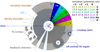 |
Fig. 1. Annotated sketch highlighting several scenarios present in an H II region around a dominant central object (DCO). Light blue arrows represent LyC photons, where an arrow ending within the extent of the H II region indicates absorption, and an arrow exceeding the region’s extent represents escape. The top left quadrant depicts the extent of H I and H II for the density- and ionisation-bounded textbook scenarios, whereas the bottom left quadrant is intended to highlight the role of a more complex gas geometry on LyC escape. The bottom right quadrant serves as a reminder that the spatial distribution of ionising sources further influences the observed LyC flux. Finally, the top right quadrant illustrates that the regions occupied by different ions vary in size, mediated by their respective ionisation potentials (an overview of the ionisation energies of a few select atoms is given in the table at the top right). |
Generally speaking, studying the properties of early galaxies remains a challenging observational task, owed to the apparent faintness and the low spatial resolution that can be achieved with present-day telescopes for such high-redshift objects. In particular, the intrinsically faint UV regime of the SED is heavily affected by extinction, and beyond redshifts of z ∼ 4, the detection of LyC photons is rendered highly unlikely due to absorption by neutral hydrogen on the line of sight (Madau & Dickinson 2014).
In order to gain further insights into the characteristics of early SFGs, a promising approach to circumvent these problems is achieved by studying local counterparts which share similar properties. Notably, the starbursts among the luminous compact galaxies (LCGs, Izotov et al. 2011) and compact SFGs (CSFGs, Izotov et al. 2021a), characterised by Hβ equivalent widths (EWs) of EW(Hβ) > 100 Å, have many commonalities to high-z SFGs, such as low metallicities, low stellar masses, and large specific star-formation rates (sSFRs). The first results from observations with the James Webb Space Telescope suggest similar findings for galaxies well in the EoR, further reinforcing the argument that the study of local analogues offers many insights into the high-z Universe (e.g. Trussler et al. 2022; Endsley et al. 2022; Schaerer et al. 2022a; Topping et al. 2022; Rhoads et al. 2023).
If SFGs were the dominant driver of reionisation, we can reasonably expect to find LCEs among such populations of local analogues. Indeed, studies of nearby, low-metallicity DGs have revealed high-ionisation nebular emission lines, such as OIII], C IV, or He II (e.g. Senchyna et al. 2017; Berg et al. 2019), requiring energies well in excess of those necessary to ionise hydrogen (13.6 eV). Not only is this another link to several high-z SFGs (e.g. Sobral et al. 2015; Stark et al. 2015; Mainali et al. 2017), but also a strong motivator for the search for LCEs among these objects, as a hard radiation field is evidently present. We would like to point out that this connection has been acknowledged before, for instance by Berg et al. (2019) and Pérez-Montero et al. (2020).
Over the last few years, a significant, albeit small sample of low-z galaxies with direct detection of LyC leakage has been compiled (Bergvall et al. 2006; Leitet et al. 2013; Borthakur et al. 2014; Leitherer et al. 2016; Izotov et al. 2016a,b, 2018a,b, 2021b; Wang et al. 2019; Malkan & Malkan 2021; Flury et al. 2022a). A particularly high detection rate of LyC escape was achieved by Izotov et al. (2016a,b) among the so-called green pea galaxies (GPs, Cardamone et al. 2009), which have been shown to be a subset of the LCGs (Izotov et al. 2011).
Whereas many LCEs do show nebular He II 4686 emission, recent works have demonstrated the absence of a correlation between spectral hardness (as traced by He II 4686/Hβ) and fesc(LyC) (Marques-Chaves et al. 2022b). This does not imply, however, that the inverse is true, and drawing a sample of SFGs from high-ionisation emission lines may yield an appreciable fraction of LCEs, which we intend to explore in this paper. This idea is further reinforced by the fact that several spectra of high redshift LCE candidates feature intense high-ionisation UV emission lines (e.g. Schaerer et al. 2022b; Naidu et al. 2022; Saxena et al. 2022).
It is to be noted that high-ionisation lines are often difficult to reproduce in spectral modelling of SFGs. Emission of He II 4686, anti-correlated with metallicity (Schaerer et al. 2019) and utilised in this work, appears to be particularly challenging. Often assumed to be a spectral signature of WR stars, Shirazi & Brinchmann (2012) found no evidence of WR stars being present in ∼40% of their He II 4686 emitting SFG sample. Similar situations arise for example in the works of Stasińska et al. (2015) and Schaerer et al. (2019), who find that current stellar models cannot reproduce the observed He II 4686 intensities, and the inclusion of non-stellar sources such as HMXBs or shocks are necessary to bring their model SEDs in line with observations.
In this work, we present our findings from legacy data of the Sloan Digital Sky Survey (SDSS, Eisenstein et al. 2011), adding a total of 18 SFGs to the list of high-z analogues, selected from their He II 4686 emission lines. Inferred from indirect tracing methods, virtually all of these galaxies are promising candidates to expand the list of local LCEs, and their recent star-formation histories (SFHs) may provide an explanation as to why their LyC radiation can escape into the IGM.
The paper is structured as follows: in Sect. 2, we describe the dataset and sample selection, while the analysis methods are covered in Sect. 3. We present the properties we derived for the galaxies we selected in Sect. 4, and summarise our results and augment them by a few concluding remarks in Sect. 5. Throughout this paper, we assume a flat ΛCDM cosmology with H0 = 67.4 km s−1 Mpc−1 and Ωm = 0.315 (Planck Collaboration VI 2020).
2. Data
2.1. Dataset
In order to obtain a sample of SFGs with He II 4686 emission, we used the Baryon Oscillation Spectroscopic Survey (BOSS, Dawson et al. 2013) dataset from the SDSS’s third run (SDSS-III, Eisenstein et al. 2011) in their twelfth data release (DR12), the final data release in the SDSS-III. The choice of this dataset is motivated by an advantage particular to DR12, as opposed to the more recent data releases, which is found in the augmentation by Thomas et al. (2013). They have published a value-added catalogue derived from fits of model spectra to the data, in which they provide refined line fluxes for the most prominent emission lines amongst other spectroscopic properties. This allows for a fairly efficient scouring of the database for the objects of our interest, whose properties are most readily derived from emission line ratios.
It is to be noted that DGs can be expected to be somewhat underrepresented in this dataset. This is evidently owed to the primary science goal of the BOSS, which has an intentional bias towards luminous, and hence massive galaxies (Dawson et al. 2013). However, their observation runs allowed for a fraction of ancillary targets deviating from their main science goal (Dawson et al. 2013), among which we deemed it likely to find suitable candidates. Previous works have demonstrated this – Guseva et al. (2017) have used this catalogue to spectroscopically identify 287 metal-deficient DG candidates, and Yang et al. (2017) extracted a sample of analogues to high-z Lyman α (Lyα) emitters by photometric selection (dubbed ‘blueberry galaxies’).
2.2. Sample selection
Typically, studies concerning SFGs utilise the presence of He II 4686 emission as an exclusion criterion (e.g. Izotov et al. 2011; Guseva et al. 2017), as this line is indicative of the presence of an AGN. However, not all He II 4686 emitters have a significant AGN contribution to their radiation field (Shirazi & Brinchmann 2012), and as we are primarily interested in finding LyC leaking galaxies, helium with its ionisation potential of 54.4 eV is chosen as an excellent indicator for the presence of a hard radiation field.
Based on SDSS DR7 data, Shirazi & Brinchmann (2012) have shown that an AGN contribution to the He II 4686 emission is negligible (< 10%) if a line ratio relation of
![Mathematical equation: $$ \begin{aligned} \log \left(\frac{{\text{ He}}{\small {{\text{ II}}}}\,4686}{\mathrm{H}\beta }\right)\le -1.22+\frac{1}{8.92\log \left({\text{[N}}{\small { {\text{ II]}}}}\,6583/\mathrm{H}\alpha \right)+1.32} \end{aligned} $$](/articles/aa/full_html/2023/04/aa45167-22/aa45167-22-eq1.gif) (1)
(1)
is satisfied. We expect this restriction to be sufficient to ensure the purity of our SFG sample with respect to AGN contamination and thus draw our final sample from Eq. (1) alone. To ensure credibility in the measured emission line fluxes, following Thomas et al. (2013), we required all objects to have an amplitude over noise (AoN) > 2 in each of the utilised emission lines.
We note that as opposed to LCGs (Izotov et al. 2011), the CSFG sample compiled in Izotov et al. (2021a) by selection allows for the presence of He II 4686 emission. Thus, at least a part of our sample is a priori likely to be a subset of the CSFGs.
3. Data analysis
3.1. Spectral analysis
After our initial sample selection, we analysed the SDSS spectra using FADO (Gomes & Papaderos 2017). In brief, this code performs a population spectral synthesis by fitting a set of simple stellar populations to a galaxy’s spectrum. FADO then reconstructs the SFH from these fits, while computing a multitude of derived galaxy properties. This principle method is well established and has been successfully applied in the past to study the physical properties of galaxies (e.g. Cid Fernandes et al. 2007). We selected FADO as our synthesis code of choice, since as opposed to other commonly used tools such as STARLIGHT (Cid Fernandes et al. 2005), FADO also accounts for the contribution of nebular continuum emission, which can be assumed to be substantial in emission line galaxies such as those studied in this work. While the overall agreement between STARLIGHT and FADO appears to be adequate, the study by Cardoso et al. (2019) particularly emphasises the better performance of FADO for (starbursting) galaxies with strong nebular emission.
Prior to the analysis, we corrected the input spectra for foreground extinction assuming a Cardelli et al. (1989) extinction curve. We assumed a standard ratio of total to selective extinction of RV ≡ AV/E(B − V) = 3.1. For each object, we adopted the V-band extinction values as listed in the NED1, taken from Schlafly & Finkbeiner (2011). Afterwards, the spectra were de-redshifted using the values provided on the website of the SDSS2.
As for our choice of the stellar populations, we adopted the models from Bruzual & Charlot (2003) in their latest version3 assuming a universal Kroupa (2001) IMF. We note that this choice is somewhat arbitrary, and the implied evolutionary parameters may be different for the stellar populations present here. In particular, as we find our objects to be compact, star-forming galaxies, binary stellar evolution may impact the galaxies’ SEDs, which is covered in the BPASS models by Stanway & Eldridge (2018). Likewise, as stated above, the results are sensitive to the choice of IMF, and it has been suggested that high-z SFGs may be governed by a top-heavy IMF (e.g. Steinhardt et al. 2022), which would have significant implications for LyC leakage (Wise & Cen 2009). As this paper is of an exploratory nature and observations of deeper optical spectra for future analysis have already been scheduled, we postpone this to a follow-up study and limit this analysis to the models by Bruzual & Charlot (2003).
In principle, these models cover a range of metallicities extending to 2.5 Z⊙, spanning 220 unequally spaced time steps from 0.1 Myr − 20 Gyr. In order to limit the range of free parameters and therefore improve the accuracy of the age estimates, we calculated preliminary oxygen abundances as outlined below (Sect. 3.2) from the emission line fluxes provided by Thomas et al. (2013). With the derived metallicities from the emission lines analysis (values in the range of Z/Z⊙ = 0.07 − 0.22), we thus limit the set of stellar populations to a total of 600 model spectra with values of Z/Z⊙ ∈ [0.005,0.02,0.2] and stellar ages of τ⋆ = 0.1 Myr − 15 Gyr.
Using this set of models, we then performed the spectral synthesis by fitting the spectral range of 3400 − 9000 Å. As we expect our objects to contain very little dust, we initially assumed negligible internal extinction, that is Aλ ∼ 0. We then consider the spectral fits by FADO as a reasonable approximation for the best (extinction-corrected) solution; in particular, the emission line fluxes found this way should be adequately corrected for underlying stellar absorption. The (emission) flux ratios of Hα, Hγ and Hδ relative to Hβ then are compared to the expected values from theory, where we consider the Case B values tabulated in Storey & Hummer (1995) for te = 15 000 K and ne = 100 cm−3 a reasonable match for the bulk of the galaxies studied here. Following Osterbrock & Ferland (2006), we then determine the extinction coefficient c(Hβ) as the mean of the extinction coefficients found for the individual line ratios, and subsequently correct the spectra assuming an SMC-like extinction law (Gordon et al. 2003, RV = 2.74). In the cases where we find a slightly negative mean value for c(Hβ), we assume no internal extinction, that is c(Hβ) = 0.
Following this, we then performed an anewed population spectral synthesis with the dereddened spectra, leaving all other parameters unchanged. During this process, FADO performed Gaussian fits for up to 51 prominent emission lines ranging from [NeV] 3426 to [FeII] 8617. After visual inspection of the spectra, we found these fits to be in very good agreement to the line fluxes observed, and hence used these values for each subsequent analysis in this work. The line fluxes along with their corresponding EWs and the derived extinction coefficients are listed in Table B.1.
For the sake of completeness, we note that FADO occassionally would shift the peak of a measured emission line by ∼1 Å bluewards. Our visual inspection of the spectra suggested that this offset had no impact on the measured fluxes, and we verified this via manual line fitting using IRAF’s (Tody 1986) splot, finding excellent agreement between the values obtained.
While FADO models a detailed SFH for each galaxy, we additionally calculated the star-formation rate (SFR) one would infer from Hα for the sake of comparability with other studies. Here, we follow Kennicutt & Evans (2012), thus logSFR(Hα) = log L(Hα) − 41.27. As our analysis (Sect. 4) reveals that the galaxies in our final sample exhibit many similarities in the properties we considered, we further produced a stack of their spectra and analysed it in the same way as the individual objects.
3.2. Abundance determination
To determine the metallicities of the objects considered here, we largely follow the prescriptions as outlined in Pérez-Montero (2017). For the determination of the oxygen abundance, we adopt the so-called ‘direct’ method, as the auroral [OIII] 4363 line is detected in all of our objects. In brief, we first calculate the electron temperature te([O III]) in the high-excitation zone from the [OIII] lines. The low-excitation zone electron temperature te([O II]) then is inferred from te([O III]) and the electron density ne, using the calibration of Hägele et al. (2006). The latter is calculated from the [SII] 6717,6731 lines whenever possible and otherwise assumed to have a value of 100 cm−3. This value is comparable to those found in the LCGs of Izotov et al. (2011), who report median electron densities between 90 cm−3 and 180 cm−3. These values, along with [OIII] 4959,5007 and [OII] 3727 = [OII] 3726,3729 fluxes then are used to determine the fractions of singly and doubly ionised oxygen relative to ionised hydrogen.
As the galaxies studied here are highly ionised, we also consider an ionisation correction factor (ICF) compensating for the neglection of O3+ in this calculation. Again following Pérez-Montero (2017), we first calculate the abundance of doubly ionised helium y2+ from He II 4686 and a weighted mean of the singly ionised helium abundance y+ from He I 4471,5876,6678,7065, under the assumption that the intrinsic attenuation is small and the optical depth function fλ(n, t, τ) (Olive & Skillman 2004) can be approximated as fλ ≈ 1 (Pérez-Montero 2017). We note that for a handful of objects, the y+ values derived from He I 6678 would deviate from the values obtained from the other He I lines by up to 12 orders of magnitude. In those cases, we excluded these unphysical values from the calculations and limit our evaluation to He I 4471,5876,7065. Using the calibrations from Pérez-Montero et al. (2020, their Appendix A), y+ and y2+ then are converted into ICF(O+ + O2+), and the total oxygen abundance is calculated as O/H = ICF(O+ + O2+)×(O+/H+ + O2+/H+).
For our preliminary oxygen abundance evaluation (see above, Sect. 3.1), this was not possible for nine objects due to the absence of reliable measurements of various required emission line fluxes in the catalogue of Thomas et al. (2013). To determine the oxygen abundance, we then used the empirical relation between oxygen abundance and te([O III]) as calibrated in Pérez-Montero et al. (2021). In case both methods were not applicable, we adopted the strong-line method by Pagel et al. (1979), also known as the R23 method. As this diagnostic is double-valued and does not allow a conclusive oxygen abundance determination in the range of 8.0 ≲ log(O/H)+12 ≲ 8.3 (Pérez-Montero 2017), we first computed a rough estimate of the metallicity from [NII] 6583/Hα (Pérez-Montero & Contini 2009), and consequently applied the upper or lower branch of the R23 method.
From the values obtained during the ICF calculations outlined above, we also determine the helium abundance, assuming that He/H = (He++He2+)/H+ = y+ + y2+. The nitrogen abundance relative to oxygen, again following Pérez-Montero (2017)4, was calculated from [NII] 6583, [OII] 3727, and te([O II]), assuming that N+/N = O+/O.
3.3. LyC leakage diagnostics
To this date, direct measurements of the LyC flux shortwards of 912 Å are the only fully reliable diagnostic for LyC leakage and derivations of fesc(LyC). However, significant efforts to relate other observable quantities to LyC escape have been made in the last few years. Particularly promising ist the study of Lyα, whose line profile is related to the ISM structure (e.g. Gronke et al. 2016), and the peak separation of the double-peaked Lyα line emerging from a clumpy ISM may relate to fesc(LyC) (Verhamme et al. 2015). Izotov et al. (2020) provide a calibration relating the Lyα escape fraction fesc(Lyα) to fesc(LyC), but caution this is a preliminary relation inferred from low sample statistics.
In case of LyC escape being realised through ionised low density tunnels in the ISM, several FUV metal absorption lines may display residual flux at their line centre (Heckman et al. 2001). As this residual flux then directly relates to the covering fraction of neutral gas, they can be used to infer a prediction for fesc(LyC) (Chisholm et al. 2018).
These diagnostics, however, require information from the ultraviolet portion of the spectrum, a wavelength range that for objects in the low-redshift regime is accessible only to the Cosmic Origins Spectrograph (COS) aboard the Hubble Space Telescope (HST). No such data is available for our objects, and even the Mg II 2796,2803 lines that provide strong evidence for the possibility of LyC escape as they trace an optically thin medium (Chisholm et al. 2020) were not or not reliably measured here.
In the optical regime, there are a few emission line diagnostics that relate to conditions favourable for LyC escape. A promising approach to look for LyC leakers is to select galaxies with large O32 = [O III] 5007/[O II] 3727 flux ratios, which indicates optically thin gas with a high degree of ionisation (Jaskot & Oey 2013), and using it as a selection criterion has lead to several successful detections of genuine LyC leakers (e.g. Izotov et al. 2016a,b, 2018a,b). Chisholm et al. (2018) even provide a tentative calibration relating this line ratio to fesc(LyC), but as Jaskot et al. (2019) note, a high O32 flux ratio alone is an insufficient LyC leakage diagnostic, as the line ratio can be modulated by the structure of the ISM. Nakajima et al. (2020) confirm that such an elevated line ratio is indeed a necessary, yet not sufficient condition for a galaxy to be a LyC leaker. Still, the results presented in Flury et al. (2022b) show that along with the (related) parameter ΣSFR, Hβ, O32 to date is the best optical diagnostic relating to fesc(LyC). A similar pre-selection of LyC leaker candidates may be possible with the [NeIII] 3869/[OII] 3727 ionisation parameter diagnostic (Levesque & Richardson 2014), which has the additional benefit of being less affected by internal reddening.
Another characteristic many LyC leakers seem to share is a deficiency in [SII] 6717,6731/Hα. Sulphur with its rather low ionisation potential of 10.36 eV causes these lines to predominantly originate in the partially ionised zone beyond the edge of the fully ionised gas, which is less pronounced in density-bounded nebulae and thus correlates with LyC leakage (Alexandroff et al. 2015). Wang et al. (2019) have demonstrated this as a powerful selection tool for LyC leaker candidates and expanded upon this diagnostic in Wang et al. (2021) with the sample of the recent Low-Redshift LyC Survey (Flury et al. 2022a), where they provide a calibration in the [OIII] 5007/Hβ vs. [SII] 6717,6731/Hα parameter space for typical emission line galaxies. A deviation in [SII] 6717,6731/Hα from this ridge line (denoted as Δ[S II]) statistically correlates with a larger fesc(LyC), even though it does not allow for an accurate determination of this parameter.
In conclusion, there is no definite, independent method to accurately predict a galaxy’s fesc(LyC) as of now, but the application of a multitude of diagnostics correlated with ionising photon loss as outlined above provide strong selection criteria for genuine LyC leakers. Here, we make use of the O32 based calibration by Chisholm et al. (2018) to obtain an estimate of fesc(LyC), that is
 (2)
(2)
An alternative calibration can be found in Izotov et al. (2018a), yielding significantly larger values of fesc(LyC) in galaxies with large O32.
4. Sample properties
4.1. Global sample characteristics
Of a total of 1 381 398 objects present in the dataset, 1504 (∼0.01%) satisfied the AoN limitation imposed upon the He II 4686, Hβ, Hα, and [NII] 6583 diagnostic lines. Within this subset, an initial sample of 22 galaxies satisfied our selection criterion given by Eq. (1). After our renewed emission-line fitting, we found that for two of those objects, the He II 4686/Hβ ratios had been understimated in the catalogue of Thomas et al. (2013), and the diagnostic by Shirazi & Brinchmann (2012) reveals these to comprise a significant AGN contribution (red diamonds in Fig. 2). Furthermore, when considering the diagnostic diagram first introduced by Baldwin et al. (1981, hereafter BPT; Fig. 3), commonly used to separate SFGs from AGN, we find the majority of the remaining objects to occupy the same region in the high-ionisation tail of the diagram. Two galaxies are found to be clearly offset from this population (yellow circles in Fig. 3) and their line ratios are more in line with those found in typical SFGs, which justifies their exclusion from our final sample. For completeness, and also as each of these outliers exhibit interesting characteristics in their own right, we discuss them in Appendix A. Our final sample now consists of 18 objects, which we dub the ionised, metal-poor galaxies (IMPs). Within the diagnostic diagram used for the selection of our sample (Fig. 2), these reside in a well-defined locus significantly offset from the bulk of He II 4686 emitters, suggesting a similar ionisation mechanism other than an AGN is prevalent in these galaxies.
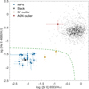 |
Fig. 2. Shirazi & Brinchmann (2012) diagram including their AGN diagnostic (green dashed line). Blue squares represent the IMPs, whereas the position of their stack is shown as a black downward-facing open triangle. Red diamonds and yellow circles mark the AGN contaminated galaxies and star-forming objects classified as outliers (see text). The grey scale density diagram represents all eligible galaxies from the SDSS DR12 with AoN > 2 in the utilised emission lines, binned in 0.02 × 0.02 dex bins for the line ratios shown. Lower contrast indicates lower bin occupancy. |
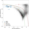 |
Fig. 3. BPT diagram including the photoionisation limit from Kewley et al. (2001, red dash-dotted line) and the AGN separation line from Kauffmann et al. (2003, green dashed line). Symbols are the same as in Fig. 2. |
To the best of our knowledge, none of these objects have previously been studied individually in the literature. We list their coordinates and redshifts along with several general properties in Table 1. For reasons of legibility, we reduce the galaxy name to the first four+four digits of the SDDS identifier.
Global properties of the galaxies studied in this work.
We find the IMPs ubiquitously reside at low redshifts (0.01 ≲ z ≲ 0.09), which can be attributed to a selection effect as we require a reliably measured He II 4686 line. All of them are readily classified as DGs, with stellar masses ranging from 6.2 ≲ log(M⋆/M⊙) ≲ 8.8. They are characterised by moderate to large sSFRs of ∼0.74 − 137 Gyr−1 with a median of ∼7.09 Gyr−1, which serves as a first indicator that the IMPs blend well into the population of LCGs and CSFGs (Izotov et al. 2011, 2021a), where similar values are reported. This likeness is further supported by the large values we find for EW(Hβ) and EW([O III] 5007) (Fig. 4), the former of which already points towards the IMPs harbouring a young starburst.
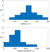 |
Fig. 4. Distribution of EW(Hβ) (top) and EW([O III] 5007) (bottom) for the IMPs, binned in 50 Å and 500 Å bins, respectively. |
4.2. Morphology
The SDSS image cutouts of the final sample are shown in Fig. 5. While most of the IMPs are only marginally resolved, they exhibit diverse morphological features. A few of them appear almost circular in projection (arguably most pronounced in J1411+0550), whereas others display signs of anisotropic extended emission. A variety of possible causes may serve to explain this, such as the galaxies’ intrinsic irregular morphology, large-scale outflows, or a recent merger, which is difficult to deduce from the SDSS images alone. Occassionally, we see more than one bright, star-forming knot (e.g. in J0006+0255, J1141+6059) which lends further credibility to a merging scenario, albeit it is equally plausible these are isolated regions of increased star-forming activity within the same galactic system.
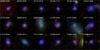 |
Fig. 5. Mosaic of the SDSS gri cutouts of our final sample obtained from the SDSS SkyServer at http://skyserver.sdss.org/. Each cutout spans a region of 12.5″ × 12.5″, where north is up and east is to the left. |
One feature all IMPs certainly appear to share is their compactness. The SDSS pipeline lists petrosian radii (r-band) between 1.43″ and 6.93″ for the IMPs, which translate to sizes of rpetro ∼ 0.52 − 5.2 kpc at their given redshifts (calculated using Ned Wright’s Cosmology Calculator, Wright 2006, with cosmological parameters from Planck Collaboration VI 2020), with a median value of rpetro ∼ 2.74 kpc. Note that most of these objects have been flagged MANYPETRO by the SDSS pipeline, meaning several possible values for rpetro were found and those listed are the maximum values. Consequently, these are best interpreted as upper limits to the true (petrosian) sizes. We further point out that for several (5/18) of the IMPs, the radii (see Table 1) exceed the 3″ fibre diameter of the BOSS spectrograph (Smee et al. 2013), hence the properties derived for these objects exclude the contribution from the galactic outskirts (to varying degrees).
Their compactness further reinforces the notion that the IMPs can be considered a subclass of the LCGs, discovered by Izotov et al. (2011). For most of the objects, the same conclusion can immediately be drawn regarding the CSFGs (Izotov et al. 2021a), which (amongst other criteria) were selected as galaxies with rpetro ≤ 3″. The conversion to linear scales of the IMPs’ radii (see Table 1) reveals these likewise are suitable objects to fulfil the compactness criterion imposed on the CSFGs.
4.3. Integrated nebular characteristics
The properties we derived from the observed emission lines (listed in Table B.1) of our sample are presented in Table 2. Particularly noteworthy is the fact that the choice of stellar population models allows FADO to successfully reproduce the He II 4686 line for all objects studied here, without any need of invoking ‘exotic’ radiative sources as discussed in the Sect. 1.
Derived properties for the galaxies in our sample as indicated in the first column.
The IMPs are ubiquitously characterised by large electron temperatures in the high-ionisation regime, with values typically found in the range of te([O III]) ∼ 12 750 − 17 670 K. As we selected the IMPs as highly ionised galaxies evident from He II 4686 emission, this is reflected in the relatively large values of the ionisation parameter-sensitive line ratio O32, spanning a range of O32 = 2.3 − 24. Considering their respective error ranges, 16 of the IMPs are consistent with a ratio of O32 > 5, a value large enough to indicate a potential escape of LyC (Izotov et al. 2016a,b, 2018a). A galaxy’s ionisation parameter can primarily be elevated by two means, them being a large intrinsic flux of ionising photons or low densities in the ISM. While the former criterion is a given here, the large scatter in O32 is suggestive of an additional mechanism influencing these values. An obvious candidate for this are density-bounded conditions, where [OII] emission is diminished. We explore this scenario further in Sect. 4.7.
The electron densities derived from [SII] are found to be consistent with the low values typically found in SFGs and lie between ne = 20 − 470 cm−3 when accounting for the full error range, subsequently justifying our assumption of ne = 100 cm−3 for the galaxies where no physically meaningful value for ne could be derived. In terms of oxygen abundance the IMPs are markedly sub-solar, with abundances ranging between 7% and 28% Z⊙ at a median of 14.4% Z⊙, assuming log(O/H)⊙ + 12 = 8.69 (Asplund et al. 2009). This is comparable to, yet slightly lower than the LCGs and CSFGs from Izotov et al. (2011, 2021a), who find median values in log(O/H) + 12 of 8.11 (26% Z⊙) and 8.0 (20% Z⊙), respectively.
The chemical enrichment history as traced by N/O exhibits no apparent peculiarities with respect to values typically found in SFGs. The relative nitrogen abundance is strongly intertwined with a galaxy’s SFH, as SNe of young, massive stars expel large amounts of oxygen into the ISM, thereby decreasing N/O. Evolved low- and intermediate-mass stars, on the other hand, can substantially increase N/O via hot bottom burning during their AGB phase (Vincenzo et al. 2016). Here, as evident from Fig. 6, the values we derived are broadly consistent with log(N/O) ∼ −1.6, where log(N/O) plateaus for low-metallicity SFGs (Vincenzo et al. 2016). In particular, the absence of a deviation towards elevated N/O values with respect to other galaxies with similar O/H suggests no dominant older stellar component is present in the IMPs. However, we note that with the large errors associated with N/O alongside the fact that other mechanisms such as gas accretion and galactic winds can alter this ratio, this conclusion remains fairly uncertain at this point.
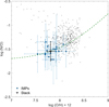 |
Fig. 6. Nitrogen vs. oxygen abundance, with symbols representing the same objects as in Fig. 2. The SDSS DR12 galaxies (black scatter diagram) are limited to SFGs with appropriate AoN in the line fluxes relevant for the determination of N/O and O/H with the direct method. The green dashed line is the generic scaling relation from Nicholls et al. (2017), i.e. log(N/O) = log(10−1.732+10logO/H + 2.19). |
The fact that the IMPs are otherwise quite extraordinary objects with respect to typical SFGs is reflected in their position in the O32 vs. R23 diagram (Fig. 7), a diagnostic diagram tracing the ionisation parameter and metallicity. Not only are they clearly offset from the bulk of the DR12 SFGs, but they also share roughly the same parameter space as many known LyC leakers, which we explore further in Sect. 4.7. Lastly, we remark that the visual inspection of the spectra suggests that at least two of the IMPs (J1311+3750 and J1608+0413) are contenders for studying the rarely detected [FeV] 4227 emission line (e.g. Thuan & Izotov 2005; Izotov et al. 2017), but as the SDSS spectra are increasingly noisy towards the blue end, we cannot claim a reliable detection with the data at hand.
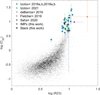 |
Fig. 7. Ionisation parameter and metallicity sensitive log(O32) = log([O III] 5007/([O III] 3727) vs. log(R23) = log(([O II] 3727 + [O III] 4959 + [O III] 5007/Hβ diagram. Symbols are the same as in Fig. 2. Additional markers were added for several low-z LyC leakers, i.e. the GPs from Izotov et al. (2016a,b, 2018a,b, green upward triangles) and low-mass galaxies from Izotov et al. (2021b, cyan left-facing triangles). Also shown are the intermediate-z LyC leakers Ion2 from de Barros et al. (2016, orange pentagram), four galaxies from Fletcher et al. (2019, dark red hexagrams, where we converted their listed [OIII] 4959,5007 values to [OIII] 5007 assuming [OIII] 5007/[OIII] 4959 = 2.98, Storey & Zeippen 2000), and AUDFs01 from Saha et al. (2020, purple right-facing triangle). The SDSS DR12 galaxies (black scatter diagram) are limited to those identified as SFGs with the BPT diagnostics from Kewley et al. (2001) and Kauffmann et al. (2003). |
4.4. Balmer decrements
A seemingly peculiar behaviour of the IMPs is found in their Balmer decrements (the line ratios of hydrogen Balmer lines relative to Hβ). Typically, one would expect these to be in good agreement to the theoretical values after accounting for internal reddening, as it is common procedure to scale the extinction law of choice by the Hβ extinction coefficient, which itself is a mean value derived from comparison of theoretically expected to observed Balmer decrements.
As evident from Fig. 8, several of the Balmer decrements in the IMPs disagree with the theoretical predictions. For reference, we show the Case A and B values derived by Storey & Hummer (1995) for ne = 100 cm−3 and te = 15 000 K, which is broadly consistent with what we found for the IMPs. We note that for the low densities present here, the assumption of tenfold higher values for ne (1000 cm−3) has virtually no effect on the line ratios. Likewise, varying the temperature by ±5000 K only moderately affects the line ratios and does not alleviate the tension presented here.
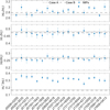 |
Fig. 8. Balmer decrements derived for the IMPs after accounting for foreground and internal extinction. The horizontal lines mark the expected theoretical values calculated by Storey & Hummer (1995) for ne = 100 cm−3 and te = 15 000 K, assuming Case A (dotted line) and Case B (dashed line) conditions. The * symbol signifies a likely blend of multiple lines (see text). |
A marked deviation to higher relative fluxes is found in Hα/Hβ, but let us consider the Balmer lines of higher order first. A significant deviation is observed in Hϵ/Hβ, where the values measured are a factor of ∼2 larger than expected. This finding has a rather straightforward explanation, as Hϵ at 3970 Å is located at roughly the same wavelength as [NeIII] 3967 and Ca II H at 3969 Å. The line fitting catalogue contained in FADO does not encompass Ca II emission, and its fitting routine would not fit the [NeIII] 3967 line in any of the objects studied here, which we ascribe to a resolution effect. The values we report here for Hϵ are thus likely a blend of Hϵ, [NeIII] 3967, and interstellar Ca II H emission, whereas the latter’s contribution is expected to be small. An additional source of uncertainty that becomes evident here is the neglection of interstellar Ca II H absorption, whose omission may negatively impact our stellar population fit. While the spectra at hand do not have the resolution sufficient to reliably disentangle these lines, by comparison to the fiducial Case B values we predict relative emission line fluxes of 100 × ([Ne III]3967 + Ca IIHem+abs)/Hβ = 9 − 20 with a median of 16 in the IMPs.
Hδ/Hβ and Hγ/Hβ appear to be skewed to slightly lower line ratios, though the median deviation from the theoretical value is reasonably small at 4.1% and 1.8%, respectively. Considering the non-quantified error sources present here, such as the choice of extinction law and its application to an integrated galactic spectrum, implicitly assuming the same extinction properties independent of the line of sight, some deviations are not unexpected. With the strongest outliers deviating in the line ratios by a mere 6.5% and 4.2%, we consider these values to be in decent agreement with the expectations.
Revisiting Hα/Hβ, we find these line ratios to be up to 8.1% larger than the reported Case B values. While the mean deviation is moderately low at ∼3.4%, about a third of our sample shows line ratios of Hα/Hβ ≳ 2.9, reminiscent of what is typically found in AGN. We note that as we find indications for an optically thin ISM throughout this paper, Case A conditions might even be the better approximation here, but this only worsens the disagreement to a median deviation of 4.5% at a maximum of 10.9%. These values are highly suggestive of an additional low-energy phenomenon that is able to elevate the electron bound by hydrogen to n = 3, resulting in a net increase in Hα flux without altering the higher-order line ratios. We speculate that collisional excitation in a large-scale galactic wind or conversely, during the accretion of large volumes of extragalactic gas, may account for this observation. Ultimately, deeper high-resolution spectra are needed to appropriately characterise the ISM dynamics that would be supportive of this argument. Alternatively, it could turn out to be an effect of technical rather than astrophysical nature, and may be the result of the best fit from population spectral synthesis being a mix of stellar populations that underpredict the total amount of stellar Hα absorption.
In Table 1 we list the recalculated (s)SFR(Hα) values denoted as (s)SFRB based on the assumption that Hα shows such an flux excess and the Case B values better represent the star-formation induced Hα flux. While this slightly diminishes the values we find (to a median sSFR of ∼7.08 Gyr−1), it does not qualitatively alter our conclusion. The same is true for the diagnostics incorporating Hα (Figs. 2 and 3).
4.5. Star-formation histories
The population synthesis by FADO reveals the IMPs to have undergone similar star formation episodes in the past. We show the mass- and luminosity-weighted SFHs of the IMPs in Figs. 9 and 10. As evident from their SFHs, the IMPs typically contain a population of old stars at ∼1 − 10 Gyr that dominate in mass. This is different for J0131+0210, J0138+1114, and J1556+1818, whose SEDs are consistent with that of a galaxy no older than ∼5 − 120 Myr.
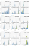 |
Fig. 9. SFHs of the first half of the IMPs. The top panel in each plot pair shows the SFH weighted by the stellar population’s luminosity at 4020 Å, whereas the bottom panel shows the mass-weighted SFH. Here, the black arrow marks the time where half of the galaxy’s mass was assembled, as indicated by the t1/2 inset. The bar colours correspond to the stellar metallicity as indicated by the numbers above each plot pair, in units of Z⊙. |
The SFHs subsequent to the formation of the old population, where present, vary from object to object. In about a third of the sample, the majority of the recent Gyr is a period of relative quiescence, whereas the other galaxies have undergone one or more bursts of star-formation during that time.
The most recent SFH, however, appears to be virtually the same for most of the IMPs: roughly 5 − 15 Myr ago, star formation in the IMPs had a major resurgence, where a young, typically luminous stellar population was formed. This then is followed by one or several bursts several Myr later, in which the currently youngest stellar generation with ages of 0.1 − 1.3 Myr was formed. In two of the IMPs (J1037+2325, J1109+3429), the youngest stellar population is less dominant with respect to those of the remaining galaxies, providing less than ∼0.1% of the galaxies’ total mass. The overall pattern, however, is the same as in the other objects.
The situation we find in the majority of the IMPs is remarkably similar to that in other metal-poor DGs, where this two-stage starburst scenario appears to be linked to superbubbles and galactic outflows, for instance in NGC 1569 (Heckman et al. 1995; Vallenari & Bomans 1996; Origlia et al. 2001) or NGC 5253 (Monreal-Ibero et al. 2010; Calzetti et al. 2015). Several LCGs, such as the GPs studied by Amorín et al. (2012), have been shown to have a similar SFH. In particular, we highlight the likeness to some well-studied (candidate) LCEs. A prominent example is ESO 338−IG04, whose SFH has been reconstructed from the study of 124 star clusters by Östlin et al. (2003). While they found a significant number of Gyr old clusters to be present, a population of massive star clusters was formed 8 − 11 Myr ago, followed by the formation of numerous young stars within the last 2 Myr. A similar situation is found in the GP analogue NGC 2366, where a 3 Myr star cluster has carved a superbubble into the ISM which is now ionised by the young < 1 Myr stellar population in the H II region Mrk 71 (Micheva et al. 2017). Tololo 1247−232 likewise was found to contain a young, two-stage starburst at 12 Myr and < 4 Myr by Micheva et al. (2018), who suggest this feature might be common in LCEs. Zastrow et al. (2013) similarly conclude that a multi-stage, young starburst may be required for the transmission of LyC radiation into the IGM.
4.6. Ionising sources
While strong He II 4686 emission is a feature typically seen in galaxies with an AGN producing a hard radiation field, we are fairly confident in excluding this possibility for the IMPs as per our selection criterion. This conclusion is further supported by the absence of spectral features characteristic of an AGN, such as broadened emission lines. Hence, it is most worthwhile to investigate the origin driving this highly energetic emission, as it may shed light on the mechanisms facilitating LyC escape in low-metallicity SFGs during the EoR.
Judging from their low oxygen abundances and large SFRs, it stands to reason that the stellar contribution to the high-energy part of the spectrum mainly comes from a young starburst. Our reconstructed SFHs from Sect. 4.5 confirm this, thus we are confident that OB stars contribute significantly to the ionisation of the ISM. However, similar to other LCGs (e.g. Amorín et al. 2012; Clarke et al. 2021), the IMPs appear to harbour older stellar populations (Sect. 4.5). Due to the exposed, hot cores of remnant stars one may reasonably expect to find here, the intrinsic LyC production in the IMPs is likely elevated by these older populations.
Features associated with WR stars, such as the ‘blue WR bump’ that one might expect at ∼4650 Å (e.g. Schaerer et al. 1999), are remarkably absent even in the stacked spectrum of the IMPs (Fig. 11, 2nd panel in the top row). There is a tentative detection of [FeIII] 4658 in this wavelength regime, but as the WR bump typically is a broad spectral feature and we furthermore detect a rather strong [FeIII] 4986 signal (see Fig. 11, bottom panel), we deem this feature likely is of nebular origin. In essence, unless a significant population of low-metallicity nitrogen WR stars (in which this feature is pronouncedly fainter than in higher-metallicity WRs, Crowther & Hadfield 2006) is present in our sample, WR stars as the origin of ionising radiation can be excluded. Further affirmation for this is found in the absence of the ‘red WR-bump’ (Fig. 11, 3rd panel in the top row), a carbon Wolf-Rayet feature of broad C IV 5808 emission (Schaerer et al. 1999). This conclusion is in line with other studies of SFGs, where the relative amount of WR stars reportedly decreases with metallicity (e.g. Guseva et al. 2000; Shirazi & Brinchmann 2012). Alternatively, as WR stars constitute a late evolutionary stage of massive stars, this again hints at the fact that the most recent starburst in the IMP galaxies is still young, which in turn further affirms that OB stars producing ionising radiation are present here.
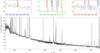 |
Fig. 11. 3400 Å–9600 Å region of the stack of eighteen redshift-corrected SDSS spectra of the IMP sample, binned in 1 Å bins and truncated in flux density f to enhance the visibility of weak spectral features (bottom row). The coloured boxes indicate the regions shown in the blow-ups in the top row, centred at [FeV] 4227, He II 4686, and C IV 5808 (blue, green, and red insets, respectively). Noteworthy emission lines (both present and absent) are marked by coloured vertical lines. The SDSS wavelengths were converted to vacuum wavelengths following Morton (1991). |
A similar argument can be made for the presence of HMXBs, as these objects require one of the binary partners to have collapsed into a compact object, such as a neutron star or a black hole. Then again, the most massive of stars evolve rapidly and are known to leave behind such compact objects at the end of their lives. Considering the most recent starbursts shown in Figs. 9 and 10, a large fraction of OB stars created at the onset of the recent star-forming episodes have already evolved into their remnant form. Thus, given a sufficient fraction of massive stars have been born in a binary configuration with an orbit close enough so that mass overflow from their companion can take place, their accretion disks can in principle contribute significant amounts of high-energy photons even in a relatively young starburst. In the case of the IMPs no archival data from Chandra or XMM-Newton is available, so we currently cannot deduce anything about the presence or absence of HMXBs. Future investigations should take this into account, as HMXBs appear to be more abundant in metal-poor dwarf galaxies and thus may contribute significantly to the ionising radiation field (Brorby et al. 2014).
Higher resolution and at best, spatially resolved data will be required to conclusively study the contribution of shocks to the ionisation of the ISM. The principle requirements for the occurence of shocks are given in star-forming regions, as kinematic phenomena with supersonic motion can for example be found in stellar winds and the expanding shells of SNe. For a preliminary evaluation, Fig. 12 shows the IMPs in three commonly used BPT diagrams, where we overplotted the model calculations from Allen et al. (2008). Shown are the tracks from their SMC model (shock front plus photoionised precursor at a pre-shock density of n = 1 cm−3), as that model at log(O/H) + 12 = 8.03 most closely matches the metallicity found in the IMPs. As evident from these diagrams, even the most favoured models with shock velocities vs = 400 km s−1 and a magnetic field of B = 10 μG predict line ratios strongly differing from the ones found in the IMPs. Given that we are considering integrated spectra, this is not surprising, as the ISM as a whole is obviously affected by a superposition of many ionising mechanisms and shocks can be expected to be more localised phenomena. Still, we can conclude that the ISM’s ionisation is unlikely to be dominated by shocks, although their contribution in supposed galactic outflow channels may be more pronounced than suggested in the diagnostics used here. Future infrared observations may aid in disentangling the shock component from the other ionisation mechanisms and provide another avenue for comparisons to high-z objects (e.g. Brinchmann 2022, and references therein).
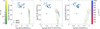 |
Fig. 12. Three commonly used BPT diagrams for shock diagnostics; symbols are the same as in Fig. 2. Solid lines show the shock+precursor SMC model grids from Allen et al. (2008) with their parameters (shock velocity vs and transverse magnetic field B) coloured as indicated by the colour bars. |
4.7. LyC leakage
The lack of UV spectra for the objects studied here makes a direct determination of their LyC escape fraction impossible. That said, the IMPs as He II 4686 emitters clearly have a significant intrinsic production of photons beyond the Lyman edge < 912 Å. This by itself already qualifies these galaxies as remarkable objects for astrophysical research, and in conjunction with the large O32 values as previously discussed makes them suitable candidates for studies concerning LyC leakage, hence we explore the possibility a little further with the optical data at hand.
To get a feel for the relevance in terms of LyC leakage, a first guess for fesc(LyC) can be obtained from Eq. (2). As pointed out in Sect. 3.3, O32 as a LyC leakage diagnostic is problematic, and the calibration from Chisholm et al. (2018) is based on low sample statistics, so we caution against an overinterpretation of the results. Performing the calculation yields LyC escape fractions between 1.4% and 98% in the IMP sample, the upper bound constituted by J1311+3750. Taken at face value, this would mean that eight of the eighteen IMPs were to be characterised by a cosmologically significant escape fraction > 10%, with eight more candidates residing at 4−10%. The fraction of strong LCEs increases to 10/18 if one utilises the O32 − fesc(LyC) relation from Izotov et al. (2018a), and all but two galaxies are found to have fesc(LyC) > 4%.
We note that the inferred LyC escape fraction of our sample shows no correlation with the relative strength of He II 4686 (Fig. 13), which is in line with the few other studies considering this potential connection (Guseva et al. 2020; Marques-Chaves et al. 2022b). As their authors have stated, this implies that the physical properties traced by He II 4686 do not govern the LyC escape fraction. However, we remark that the IMPs show considerably larger He II 4686/Hβ ratios than most established LCEs. Considering these galaxies selected as He II emitters show strong indications for appreciable escape fractions, we suggest that a mechanism responsible for the detectability of He II may be related to LyC escape. Considering that the bulk of He II emission will originate close to the sources of hard radiation, an efficient removal of neutral gas is a strong contender here, which we explore further below.
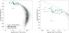 |
Fig. 13. Spectral hardness as traced by He II 4686/Hβ vs. LyC escape fraction fesc(LyC). Blue squares represent the IMPs, whereas the position of their stack is shown as a black downward-facing open triangle. We show no error bars in fesc(LyC), as the values we infer are mere estimates from O32. The stacks from the Low-redshift Lyman Continuum Leaker Survey as provided in Marques-Chaves et al. (2022b) are shown as orange circles, and the LCEs studied in Guseva et al. (2020) as green diamonds. |
The indications for LyC leakage in the IMPs are further reinforced by the strong deficit in [S II] 6717,6731/Hα with respect to typical SFGs, and following the definition of Wang et al. (2021), they span a range between Δ[S II] = 0.026 and −0.82 (Table 2). The markedly negative values indicate that large volumes in the IMPs may be density-bounded, and as such provide conditions strongly favourable for LyC leakage. Figure 14 shows their position in the plot as worked out in Wang et al. (2021) alongside with a few other known LyC leakers, demonstrating their similarity in this parameter space.
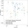 |
Fig. 14. log([O III]5007/Hβ) vs. log([S II] 6717,6731/Hα) diagram including the [SII] ridge line from Wang et al. (2021, green dashed line). Symbols are the same as in Fig. 7. Left: panel highlighting the IMPs’ positions in the parameter space covered by SDSS DR12 galaxies. Right: zoom-in on the region occupied by the IMPs. |
In principle, such conditions could likewise arise in an ionisation-bounded nebula, given a hard enough radiation field such that the inner regions where the higher-ionisation emission lines originate span a larger spatial extent and as such, dominate the line flux ratio relative to that of a lower ionisation species. If this were the case, the [SII] deficiency could be the result of most of the sulphur being doubly ionised. In the spectra of the IMPs, we detect both [SIII] 9069 and [SIII] 9531 lines (redshift permitting). While some variation is present, the overall ratio of S32 = ([S III] 9069 +[S III] 9531/[S II] 6717,6731 shows no obvious excess. For our stacked spectrum, we find logS32 ∼ 0.3, which at log([O III] 5007/Hβ) ∼ 0.94 appears to be compatible with the extrapolation of the running median of z = 0 SFGs as presented in Sanders et al. (2020, their Fig. 4). Judging from this, we conclude that our previous findings are primarily governed by the ISM structure rather than the hardness of the radiation field.
Equally remarkable is the area the IMPs reside in when comparing the two best optical LyC leakage indications, O32 and Δ[S II] (Fig. 15), also adapted from Wang et al. (2021). Here, the IMPs are well offset from the bulk of the DR12 galaxies, and roughly occupy the same region as many confirmed local LyC leakers. While Wang et al. (2021) report no statistically significant correlation between a galaxy’s fesc(LyC) and log(O32) vs. Δ[S II], it is evident that galaxies with large escape fractions generally reside in the upper left of this diagram (Wang et al. 2021, their Fig. 3), which is equally true for the IMPs.
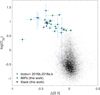 |
Fig. 15. log(O32) =log([O III] 5007/([O II] 3727) vs. Δ[S II] diagram. Symbols are the same as in Fig. 7. |
Our reconstruction of the SFHs (Sect. 4.5) offers a tempting explanation how these conditions may have come to be. While the IMPs appear to actively form young stars, a major burst in star formation has occured within the last ∼10 Myr in a majority of these objects. Within the timespan following this burst, all newly formed massive stars have since exploded as SNe, which constitutes a kinematic phenomenon that may have driven a significant fraction of the galaxies’ ISM out of their shallow potential wells. The ionising photons provided by the younger stellar generation, whose formation process may well have been triggered by or benefitted from these SN shock waves, will then find ISM conditions strongly favourable for their transmission into the IGM.
While some of the IMPs apparently lack the 10 Myr population, their youngest stellar generation is systematically more massive than that of the two-stage starburst galaxies. Here, the increased ionising flux due to the larger number of OB stars (relative to galaxy mass) may be responsible for a reduction in the neutral gas fraction in these galaxies. Alternatively, the larger number of SNe from massive (O) stars may already have provided ISM conditions similar to what we deduced for the rest of the IMPs.
Our attempts to fit an additional broad Gaussian component to some of the stronger emission lines (e.g. Hα, [OIII] 5007) did not yield any appreciable results. If such a component, indicative of a large-scale outflow (e.g. Castaneda et al. 1990), is present in the spectra of the IMPs, deeper observations are required for its detection. In about half of our sample, we can reproduce the Hα and [OIII] 5007 lines with a double-Gaussian fit, where the peak separations indicate a velocity of ∼80 km s−1 in the blue-shifted component. For an unambiguous detection of these components, however, higher resolution spectra are needed.
5. Summary and conclusion
By applying a single selection criterion based on the He II 4686 recombination line (Eq. (1)), we have extracted a sample of twenty galaxies from the SDSS DR12. Their position in the BPT diagram (Fig. 3) reveals that eighteen (90%) of these are clustered together in the respective parameter space, suggesting simliar inherent properties, which our subsequent analysis confirms. These previously undiscussed galaxies, dubbed ‘IMPs’, are revealed to be metal-poor, star-forming dwarf galaxies. Their highly ionised ISM appears to be predominantly photoionised by a young stellar population, with an additional contribution of an older (1 − 10 Gyr), evolved population in most of the galaxies. A dominant contribution from AGN, shocks, and WR stars can be ruled out at this stage, whereas the presence or absence of HMXBs remains an open question for now.
We find the IMPs with their low stellar masses, large sSFRs and markedly sub-solar metallicity blend well into the local populations of LCGs and CSFGs (Izotov et al. 2011, 2021a), which share many properties with high-z SFGs. This likeness is further reinforced by their large values in EW(Hβ) and EW([O III] 5007) along with their compact morphology. In all of these properties, however, the IMPs typically occupy the tail of the distribution found in the CSFGs, them being low-mass, low-metallicity objects with emission lines of large EWs, implying these galaxies are fairly extreme objects among the population of local analogues to high-z SFGs. This is notably similar to the CSFG subset constituted by the ‘blueberry galaxies’, which themselves are low-z LCE candidates with log(M⋆/M⊙) ∼ 7 and log(O/H) + 12 ∼ 7.7 (Yang et al. 2017).
Judging from the elevated O32 values and pronounced [SII] deficiency, our results strongly point towards large density-bounded volumes of ISM within the IMPs. This leads us to suspect that a majority of them are very likely LyC leakers, making them excellent candidates for follow-up studies with respect to LyC photon loss. Ultimately, future acquisition of spectroscopic FUV data is inevitable to unequivocally confirm this. Direct detection of LyC radiation will require the next generation of FUV instruments, though, as the sensitivity curve of HST’s COS does not permit the detection of faint LyC at these low redshifts.
The IMPs’ recent SFHs are found to be similar and offer a tempting scenario that may explain how conditions favourable for LyC leakage have come to be. Most of the galaxies have formed a stellar population which constitutes ∼0.1%−10% of their total stellar mass some 5 − 15 Myr ago. This timescale is sufficient for the massive stars of this population to have exploded as SNe by now, and the kinetic energy injected into the surrounding matter by these may have served as a mechanism for clearing low-density cavities in the ISM, through which LyC photons then may ultimately escape into the IGM.
If found to be true, these galaxies then would constitute the most close-by LyC leakers, in parts only superseded by Haro 11 (Bergvall et al. 2006), Mrk 54 (Leitherer et al. 2016) and Tol 1247−232 (Leitet et al. 2013). Moreover, it would demonstrate the validity of using high-ionisation nebular lines as a selection criterion in search of LCEs. Our O32-based estimates of fesc(LyC) suggest a detection rate of significant (> 10%) escape fractions for at least eight (40%) of the studied SFGs, though the [SII] deficient nebular emission indicates that the remaining galaxies likewise are good LCE candidates.
https://ned.ipac.caltech.edu/
https://www.sdss.org/
https://www.bruzual.org/bc03/Updated_version_2016/
We note that the prescription in Pérez-Montero (2017, their Eq. (51)) includes a typo in the second-to-last summand, where 0.687 te([O II])−1 should be a subtrahend rather than a factor.
Acknowledgments
Many thanks go to our anonymous referee, whose diligent report greatly improved the quality of this paper. The authors would like to express their gratitude towards P. Papaderos for providing further insights into the inner workings of FADO. Additionally, we thank L. Dirks for many helpful discussions. A.U.E., D.J.B. and A.W. acknowledge funding from the German Science Foundation DFG, via the Collaborative Research Center SFB1491 ‘Cosmic Interacting Matters – From Source to Signal’. This research has been made possible due to the immense data collected in the SDSS project. Funding for SDSS-III has been provided by the Alfred P. Sloan Foundation, the Participating Institutions, the National Science Foundation, and the US Department of Energy Office of Science. The SDSS-III website is http://www.sdss3.org/. SDSS-III is managed by the Astrophysical Research Consortium for the Participating Institutions of the SDSS-III Collaboration including the University of Arizona, the Brazilian Participation Group, Brookhaven National Laboratory, Carnegie Mellon University, University of Florida, the French Participation Group, the German Participation Group, Harvard University, the Instituto de Astrofisica de Canarias, the Michigan State/Notre Dame/JINA Participation Group, Johns Hopkins University, Lawrence Berkeley National Laboratory, Max Planck Institute for Astrophysics, Max Planck Institute for Extraterrestrial Physics, New Mexico State University, New York University, Ohio State University, Pennsylvania State University, University of Portsmouth, Princeton University, the Spanish Participation Group, University of Tokyo, University of Utah, Vanderbilt University, University of Virginia, University of Washington, and Yale University. This research has made use of the NASA/IPAC Extragalactic Database (NED), which is funded by the National Aeronautics and Space Administration and operated by the California Institute of Technology. All plots in this paper have been created with MATLAB R2021b (https://mathworks.com/products/matlab.html), except those in Figs. 9 and 10, which are part of the default FADO output.
References
- Alexandroff, R. M., Heckman, T. M., Borthakur, S., Overzier, R., & Leitherer, C. 2015, ApJ, 810, 104 [Google Scholar]
- Allen, M. G., Groves, B. A., Dopita, M. A., Sutherland, R. S., & Kewley, L. J. 2008, ApJS, 178, 20 [Google Scholar]
- Amorín, R., Pérez-Montero, E., Vílchez, J. M., & Papaderos, P. 2012, ApJ, 749, 185 [CrossRef] [Google Scholar]
- Asplund, M., Grevesse, N., Sauval, A. J., & Scott, P. 2009, ARA&A, 47, 481 [NASA ADS] [CrossRef] [Google Scholar]
- Baldwin, J. A., Phillips, M. M., & Terlevich, R. 1981, PASP, 93, 5 [Google Scholar]
- Behrens, C., Dijkstra, M., & Niemeyer, J. C. 2014, A&A, 563, A77 [NASA ADS] [CrossRef] [EDP Sciences] [Google Scholar]
- Berg, D. A., Chisholm, J., Erb, D. K., et al. 2019, ApJ, 878, L3 [NASA ADS] [CrossRef] [Google Scholar]
- Bergvall, N., Zackrisson, E., Andersson, B. G., et al. 2006, A&A, 448, 513 [NASA ADS] [CrossRef] [EDP Sciences] [Google Scholar]
- Binette, L., Magris, C. G., Stasińska, G., & Bruzual, A. G. 1994, A&A, 292, 13 [NASA ADS] [Google Scholar]
- Borthakur, S., Heckman, T. M., Leitherer, C., & Overzier, R. A. 2014, Science, 346, 216 [Google Scholar]
- Brinchmann, J. 2022, MNRAS, submitted [arXiv:2208.07467] [Google Scholar]
- Brorby, M., Kaaret, P., & Prestwich, A. 2014, MNRAS, 441, 2346 [NASA ADS] [CrossRef] [Google Scholar]
- Bruzual, G., & Charlot, S. 2003, MNRAS, 344, 1000 [NASA ADS] [CrossRef] [Google Scholar]
- Calzetti, D., Johnson, K. E., Adamo, A., et al. 2015, ApJ, 811, 75 [CrossRef] [Google Scholar]
- Cardamone, C., Schawinski, K., Sarzi, M., et al. 2009, MNRAS, 399, 1191 [NASA ADS] [CrossRef] [Google Scholar]
- Cardelli, J. A., Clayton, G. C., & Mathis, J. S. 1989, ApJ, 345, 245 [Google Scholar]
- Cardoso, L. S. M., Gomes, J. M., & Papaderos, P. 2019, A&A, 622, A56 [NASA ADS] [CrossRef] [EDP Sciences] [Google Scholar]
- Castaneda, H. O., Vilchez, J. M., & Copetti, M. V. F. 1990, ApJ, 365, 164 [NASA ADS] [CrossRef] [Google Scholar]
- Cen, R., & Kimm, T. 2015, ApJ, 801, L25 [Google Scholar]
- Chisholm, J., Gazagnes, S., Schaerer, D., et al. 2018, A&A, 616, A30 [NASA ADS] [CrossRef] [EDP Sciences] [Google Scholar]
- Chisholm, J., Prochaska, J. X., Schaerer, D., Gazagnes, S., & Henry, A. 2020, MNRAS, 498, 2554 [CrossRef] [Google Scholar]
- Cid Fernandes, R., Mateus, A., Sodré, L., Stasińska, G., & Gomes, J. M. 2005, MNRAS, 358, 363 [Google Scholar]
- Cid Fernandes, R., Asari, N. V., Sodré, L., et al. 2007, MNRAS, 375, L16 [NASA ADS] [CrossRef] [Google Scholar]
- Clarke, L., Scarlata, C., Mehta, V., et al. 2021, ApJ, 912, L22 [NASA ADS] [CrossRef] [Google Scholar]
- Crowther, P. A., & Hadfield, L. J. 2006, A&A, 449, 711 [NASA ADS] [CrossRef] [EDP Sciences] [Google Scholar]
- Dawson, K. S., Schlegel, D. J., Ahn, C. P., et al. 2013, AJ, 145, 10 [Google Scholar]
- de Barros, S., Vanzella, E., Amorín, R., et al. 2016, A&A, 585, A51 [NASA ADS] [CrossRef] [EDP Sciences] [Google Scholar]
- Dopita, M. A., & Sutherland, R. S. 1996, ApJS, 102, 161 [Google Scholar]
- Eisenstein, D. J., Weinberg, D. H., Agol, E., et al. 2011, AJ, 142, 72 [Google Scholar]
- Eldridge, J. J., & Stanway, E. R. 2009, MNRAS, 400, 1019 [NASA ADS] [CrossRef] [Google Scholar]
- Endsley, R., Stark, D. P., Whitler, L., et al. 2022, ArXiv e-prints [arXiv:2208.14999] [Google Scholar]
- Fan, X., Carilli, C. L., & Keating, B. 2006, ARA&A, 44, 415 [Google Scholar]
- Finkelstein, S. L., D’Aloisio, A., Paardekooper, J.-P., et al. 2019, ApJ, 879, 36 [Google Scholar]
- Fletcher, T. J., Tang, M., Robertson, B. E., et al. 2019, ApJ, 878, 87 [Google Scholar]
- Flury, S. R., Jaskot, A. E., Ferguson, H. C., et al. 2022a, ApJS, 260, 1 [NASA ADS] [CrossRef] [Google Scholar]
- Flury, S. R., Jaskot, A. E., Ferguson, H. C., et al. 2022b, ApJ, 930, 126 [NASA ADS] [CrossRef] [Google Scholar]
- Garnett, D. R., Kennicutt, R. C., Jr, Chu, Y.-H., & Skillman, E. D. 1991, ApJ, 373, 458 [NASA ADS] [CrossRef] [Google Scholar]
- Gomes, J. M., & Papaderos, P. 2017, A&A, 603, A63 [NASA ADS] [CrossRef] [EDP Sciences] [Google Scholar]
- Gordon, K. D., Clayton, G. C., Misselt, K. A., Landolt, A. U., & Wolff, M. J. 2003, ApJ, 594, 279 [NASA ADS] [CrossRef] [Google Scholar]
- Gronke, M., Dijkstra, M., McCourt, M., & Oh, S. P. 2016, ApJ, 833, L26 [CrossRef] [Google Scholar]
- Guseva, N. G., Izotov, Y. I., & Thuan, T. X. 2000, ApJ, 531, 776 [NASA ADS] [CrossRef] [Google Scholar]
- Guseva, N. G., Izotov, Y. I., Fricke, K. J., & Henkel, C. 2017, A&A, 599, A65 [NASA ADS] [CrossRef] [EDP Sciences] [Google Scholar]
- Guseva, N. G., Izotov, Y. I., Schaerer, D., et al. 2020, MNRAS, 497, 4293 [CrossRef] [Google Scholar]
- Haardt, F., & Madau, P. 2012, ApJ, 746, 125 [Google Scholar]
- Hägele, G. F., Pérez-Montero, E., Díaz, Á. I., Terlevich, E., & Terlevich, R. 2006, MNRAS, 372, 293 [CrossRef] [Google Scholar]
- Heckman, T. M., Dahlem, M., Lehnert, M. D., et al. 1995, ApJ, 448, 98 [NASA ADS] [CrossRef] [Google Scholar]
- Heckman, T. M., Sembach, K. R., Meurer, G. R., et al. 2001, ApJ, 558, 56 [Google Scholar]
- Heckman, T. M., Borthakur, S., Overzier, R., et al. 2011, ApJ, 730, 5 [Google Scholar]
- Hopkins, A. M., & Beacom, J. F. 2006, ApJ, 651, 142 [NASA ADS] [CrossRef] [Google Scholar]
- Izotov, Y. I., Guseva, N. G., & Thuan, T. X. 2011, ApJ, 728, 161 [NASA ADS] [CrossRef] [Google Scholar]
- Izotov, Y. I., Orlitová, I., Schaerer, D., et al. 2016a, Nature, 529, 178 [Google Scholar]
- Izotov, Y. I., Schaerer, D., Thuan, T. X., et al. 2016b, MNRAS, 461, 3683 [Google Scholar]
- Izotov, Y. I., Thuan, T. X., & Guseva, N. G. 2017, MNRAS, 471, 548 [NASA ADS] [CrossRef] [Google Scholar]
- Izotov, Y. I., Schaerer, D., Worseck, G., et al. 2018a, MNRAS, 474, 4514 [Google Scholar]
- Izotov, Y. I., Worseck, G., Schaerer, D., et al. 2018b, MNRAS, 478, 4851 [Google Scholar]
- Izotov, Y. I., Schaerer, D., Worseck, G., et al. 2020, MNRAS, 491, 468 [NASA ADS] [CrossRef] [Google Scholar]
- Izotov, Y. I., Guseva, N. G., Fricke, K. J., et al. 2021a, A&A, 646, A138 [NASA ADS] [CrossRef] [EDP Sciences] [Google Scholar]
- Izotov, Y. I., Worseck, G., Schaerer, D., et al. 2021b, MNRAS, 503, 1734 [NASA ADS] [CrossRef] [Google Scholar]
- Jaskot, A. E., & Oey, M. S. 2013, ApJ, 766, 91 [Google Scholar]
- Jaskot, A. E., Dowd, T., Oey, M. S., Scarlata, C., & McKinney, J. 2019, ApJ, 885, 96 [Google Scholar]
- Kauffmann, G., Heckman, T. M., Tremonti, C., et al. 2003, MNRAS, 346, 1055 [Google Scholar]
- Keenan, R. P., Oey, M. S., Jaskot, A. E., & James, B. L. 2017, ApJ, 848, 12 [NASA ADS] [CrossRef] [Google Scholar]
- Kennicutt, R. C., & Evans, N. J. 2012, ARA&A, 50, 531 [NASA ADS] [CrossRef] [Google Scholar]
- Kewley, L. J., Dopita, M. A., Sutherland, R. S., Heisler, C. A., & Trevena, J. 2001, ApJ, 556, 121 [Google Scholar]
- Kroupa, P. 2001, MNRAS, 322, 231 [NASA ADS] [CrossRef] [Google Scholar]
- Kulkarni, G., Worseck, G., & Hennawi, J. F. 2019, MNRAS, 488, 1035 [Google Scholar]
- Leitet, E., Bergvall, N., Hayes, M., Linné, S., & Zackrisson, E. 2013, A&A, 553, A106 [NASA ADS] [CrossRef] [EDP Sciences] [Google Scholar]
- Leitherer, C., Hernandez, S., Lee, J. C., & Oey, M. S. 2016, ApJ, 823, 64 [Google Scholar]
- Levesque, E. M., & Richardson, M. L. A. 2014, ApJ, 780, 100 [Google Scholar]
- Madau, P., & Dickinson, M. 2014, ARA&A, 52, 415 [Google Scholar]
- Madau, P., & Haardt, F. 2015, ApJ, 813, L8 [Google Scholar]
- Mainali, R., Kollmeier, J. A., Stark, D. P., et al. 2017, ApJ, 836, L14 [Google Scholar]
- Malkan, M. A., & Malkan, B. K. 2021, ApJ, 909, 92 [NASA ADS] [CrossRef] [Google Scholar]
- Marques-Chaves, R., Schaerer, D., Álvarez-Márquez, J., et al. 2021, MNRAS, 507, 524 [NASA ADS] [CrossRef] [Google Scholar]
- Marques-Chaves, R., Schaerer, D., Álvarez-Márquez, J., et al. 2022a, MNRAS, 517, 2972 [CrossRef] [Google Scholar]
- Marques-Chaves, R., Schaerer, D., Amorín, R. O., et al. 2022b, A&A, 663, L1 [NASA ADS] [CrossRef] [EDP Sciences] [Google Scholar]
- McGreer, I. D., Jiang, L., Fan, X., et al. 2013, ApJ, 768, 105 [NASA ADS] [CrossRef] [Google Scholar]
- McGreer, I. D., Mesinger, A., & D’Odorico, V. 2015, MNRAS, 447, 499 [NASA ADS] [CrossRef] [Google Scholar]
- Micheva, G., Oey, M. S., Jaskot, A. E., & James, B. L. 2017, ApJ, 845, 165 [NASA ADS] [CrossRef] [Google Scholar]
- Micheva, G., Oey, M. S., Keenan, R. P., Jaskot, A. E., & James, B. L. 2018, ApJ, 867, 2 [NASA ADS] [CrossRef] [Google Scholar]
- Mitra, S., Choudhury, T. R., & Ferrara, A. 2018, MNRAS, 473, 1416 [Google Scholar]
- Monreal-Ibero, A., Vílchez, J. M., Walsh, J. R., & Muñoz-Tuñón, C. 2010, A&A, 517, A27 [NASA ADS] [CrossRef] [EDP Sciences] [Google Scholar]
- Morton, D. C. 1991, ApJS, 77, 119 [Google Scholar]
- Naidu, R. P., Tacchella, S., Mason, C. A., et al. 2020, ApJ, 892, 109 [NASA ADS] [CrossRef] [Google Scholar]
- Naidu, R. P., Matthee, J., Oesch, P. A., et al. 2022, MNRAS, 510, 4582 [CrossRef] [Google Scholar]
- Nakajima, K., & Ouchi, M. 2014, MNRAS, 442, 900 [Google Scholar]
- Nakajima, K., Ellis, R. S., Robertson, B. E., Tang, M., & Stark, D. P. 2020, ApJ, 889, 161 [NASA ADS] [CrossRef] [Google Scholar]
- Nicholls, D. C., Sutherland, R. S., Dopita, M. A., Kewley, L. J., & Groves, B. A. 2017, MNRAS, 466, 4403 [Google Scholar]
- Olive, K. A., & Skillman, E. D. 2004, ApJ, 617, 29 [NASA ADS] [CrossRef] [Google Scholar]
- Origlia, L., Leitherer, C., Aloisi, A., Greggio, L., & Tosi, M. 2001, AJ, 122, 815 [NASA ADS] [CrossRef] [Google Scholar]
- Osterbrock, D. E., & Ferland, G. J. 2006, Astrophysics of Gaseous Nebulae and Active Galactic Nuclei (Sausalito: University Science Books) [Google Scholar]
- Östlin, G., Zackrisson, E., Bergvall, N., & Rönnback, J. 2003, A&A, 408, 887 [NASA ADS] [CrossRef] [EDP Sciences] [Google Scholar]
- Ouchi, M., Mobasher, B., Shimasaku, K., et al. 2009, ApJ, 706, 1136 [NASA ADS] [CrossRef] [Google Scholar]
- Pagel, B. E. J., Edmunds, M. G., Blackwell, D. E., Chun, M. S., & Smith, G. 1979, MNRAS, 189, 95 [NASA ADS] [CrossRef] [Google Scholar]
- Pérez-Montero, E. 2017, PASP, 129, 043001 [CrossRef] [Google Scholar]
- Pérez-Montero, E., & Contini, T. 2009, MNRAS, 398, 949 [CrossRef] [Google Scholar]
- Pérez-Montero, E., Kehrig, C., Vílchez, J. M., et al. 2020, A&A, 643, A80 [NASA ADS] [CrossRef] [EDP Sciences] [Google Scholar]
- Pérez-Montero, E., Amorín, R., Sánchez Almeida, J., et al. 2021, MNRAS, 504, 1237 [CrossRef] [Google Scholar]
- Planck Collaboration VI. 2020, A&A, 641, A6 [NASA ADS] [CrossRef] [EDP Sciences] [Google Scholar]
- Plat, A., Charlot, S., Bruzual, G., et al. 2019, MNRAS, 490, 978 [Google Scholar]
- Rhoads, J. E., Wold, I. G. B., Harish, S., et al. 2023, ApJ, 942, L14 [NASA ADS] [CrossRef] [Google Scholar]
- Robertson, B. E., Furlanetto, S. R., Schneider, E., et al. 2013, ApJ, 768, 71 [Google Scholar]
- Robertson, B. E., Ellis, R. S., Furlanetto, S. R., & Dunlop, J. S. 2015, ApJ, 802, L19 [Google Scholar]
- Saha, K., Tandon, S. N., Simmonds, C., et al. 2020, Nat. Astron., 4, 1185 [NASA ADS] [CrossRef] [Google Scholar]
- Sana, H., de Mink, S. E., de Koter, A., et al. 2012, Science, 337, 444 [Google Scholar]
- Sanders, R. L., Jones, T., Shapley, A. E., et al. 2020, ApJ, 888, L11 [Google Scholar]
- Saxena, A., Cryer, E., Ellis, R. S., et al. 2022, MNRAS, 517, 1098 [Google Scholar]
- Schaerer, D. 1996, ApJ, 467, L17 [NASA ADS] [CrossRef] [Google Scholar]
- Schaerer, D. 2002, A&A, 382, 28 [NASA ADS] [CrossRef] [EDP Sciences] [Google Scholar]
- Schaerer, D. 2003, A&A, 397, 527 [NASA ADS] [CrossRef] [EDP Sciences] [Google Scholar]
- Schaerer, D., Contini, T., & Kunth, D. 1999, A&A, 341, 399 [NASA ADS] [Google Scholar]
- Schaerer, D., Fragos, T., & Izotov, Y. I. 2019, A&A, 622, L10 [NASA ADS] [CrossRef] [EDP Sciences] [Google Scholar]
- Schaerer, D., Marques-Chaves, R., Barrufet, L., et al. 2022a, A&A, 665, L4 [NASA ADS] [CrossRef] [EDP Sciences] [Google Scholar]
- Schaerer, D., Izotov, Y. I., Worseck, G., et al. 2022b, A&A, 658, L11 [NASA ADS] [CrossRef] [EDP Sciences] [Google Scholar]
- Schlafly, E. F., & Finkbeiner, D. P. 2011, ApJ, 737, 103 [Google Scholar]
- Senchyna, P., Stark, D. P., Vidal-García, A., et al. 2017, MNRAS, 472, 2608 [NASA ADS] [CrossRef] [Google Scholar]
- Sharma, M., Theuns, T., Frenk, C., et al. 2016, MNRAS, 458, L94 [CrossRef] [Google Scholar]
- Shirazi, M., & Brinchmann, J. 2012, MNRAS, 421, 1043 [NASA ADS] [CrossRef] [Google Scholar]
- Smee, S. A., Gunn, J. E., Uomoto, A., et al. 2013, AJ, 146, 32 [Google Scholar]
- Smith, L. J., Norris, R. P. F., & Crowther, P. A. 2002, MNRAS, 337, 1309 [CrossRef] [Google Scholar]
- Sobral, D., Matthee, J., Darvish, B., et al. 2015, ApJ, 808, 139 [Google Scholar]
- Stanway, E. R., & Eldridge, J. J. 2018, MNRAS, 479, 75 [NASA ADS] [CrossRef] [Google Scholar]
- Stark, D. P. 2016, ARA&A, 54, 761 [Google Scholar]
- Stark, D. P., Walth, G., Charlot, S., et al. 2015, MNRAS, 454, 1393 [Google Scholar]
- Stasińska, G., Izotov, Y., Morisset, C., & Guseva, N. 2015, A&A, 576, A83 [NASA ADS] [CrossRef] [EDP Sciences] [Google Scholar]
- Steinhardt, C. L., Sneppen, A., Mostafa, B., et al. 2022, ApJ, 931, 58 [NASA ADS] [CrossRef] [Google Scholar]
- Storey, P. J., & Hummer, D. G. 1995, MNRAS, 272, 41 [NASA ADS] [CrossRef] [Google Scholar]
- Storey, P. J., & Zeippen, C. J. 2000, MNRAS, 312, 813 [NASA ADS] [CrossRef] [Google Scholar]
- Thomas, D., Steele, O., Maraston, C., et al. 2013, MNRAS, 431, 1383 [NASA ADS] [CrossRef] [Google Scholar]
- Thuan, T. X., & Izotov, Y. I. 2005, ApJS, 161, 240 [NASA ADS] [CrossRef] [Google Scholar]
- Tody, D. 1986, in Instrumentation in Astronomy VI, ed. D. L. Crawford, SPIE Conf. Ser., 627, 733 [NASA ADS] [CrossRef] [Google Scholar]
- Topping, M. W., Stark, D. P., Endsley, R., et al. 2022, ApJ, 941, 153 [NASA ADS] [CrossRef] [Google Scholar]
- Trussler, J. A. A., Adams, N. J., Conselice, C. J., et al. 2022, ArXiv e-prints [arXiv:2207.14265] [Google Scholar]
- Vallenari, A., & Bomans, D. J. 1996, A&A, 313, 713 [NASA ADS] [Google Scholar]
- Verhamme, A., Orlitová, I., Schaerer, D., & Hayes, M. 2015, A&A, 578, A7 [NASA ADS] [CrossRef] [EDP Sciences] [Google Scholar]
- Vincenzo, F., Belfiore, F., Maiolino, R., Matteucci, F., & Ventura, P. 2016, MNRAS, 458, 3466 [NASA ADS] [CrossRef] [Google Scholar]
- Wang, B., Heckman, T. M., Leitherer, C., et al. 2019, ApJ, 885, 57 [NASA ADS] [CrossRef] [Google Scholar]
- Wang, B., Heckman, T. M., Amorín, R., et al. 2021, ApJ, 916, 3 [NASA ADS] [CrossRef] [Google Scholar]
- Wise, J. H., & Cen, R. 2009, ApJ, 693, 984 [NASA ADS] [CrossRef] [Google Scholar]
- Wise, J. H., Demchenko, V. G., Halicek, M. T., et al. 2014, MNRAS, 442, 2560 [NASA ADS] [CrossRef] [Google Scholar]
- Wright, E. L. 2006, PASP, 118, 1711 [NASA ADS] [CrossRef] [Google Scholar]
- Yang, H., Malhotra, S., Rhoads, J. E., & Wang, J. 2017, ApJ, 847, 38 [NASA ADS] [CrossRef] [Google Scholar]
- Zackrisson, E., Inoue, A. K., & Jensen, H. 2013, ApJ, 777, 39 [NASA ADS] [CrossRef] [Google Scholar]
- Zastrow, J., Oey, M. S., Veilleux, S., & McDonald, M. 2013, ApJ, 779, 76 [NASA ADS] [CrossRef] [Google Scholar]
Appendix A: Outlier galaxies
In this section we briefly discuss the four outlier galaxies we removed from our final sample. In Figs. A.1 and A.2 we reproduce our SFG/AGN diagnostic diagrams (Figs. 2 and 3) to clarify the positions of the individual objects in the plot. Their general characteristics are listed in Table A.1, while Table A.2 contains the derived nebular characteristics considered in this work.
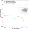 |
Fig. A.1. Same as Fig. 2, highlighting three of the four outlier galaxies removed from our sample as indicated in the plot legend. |
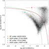 |
Fig. A.2. Same as Fig. 3, highlighting the four outlier galaxies removed from our sample as indicated in the plot legend. |
Same as Table 1, but for the four galaxies identified as outliers.
Same as Table 2, but for the four galaxies identified as outliers.
Additionally, we reproduce the shock diagnostic plot for the outliers in Fig. A.4 alongside the LMC tracks from Allen et al. (2008), as they are a better match in metallicity (log(O/H) + 12 = 8.35) for most objects considered here. Due to these higher metallicities, we have additionally incorporated 200 simple stellar populations of ages between 0.1 Myr and 15 Gyr at a metallicity of Z/Z⊙ = 0.4 during the analysis with FADO. The outliers’ emission line fluxes can be found in Table B.2. Figure A.3 shows the SDSS gri composite images of the galaxies in the same order as we discuss them in the subsequent sections.
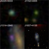 |
Fig. A.3. Same as Fig. 5 for the four galaxies identified as outliers. The last panel is zoomed out by a factor of 10, i.e. spanning a region of 125″ × 125″. |
A.1. SF outlier: J0225+0033
J0225+0033 is one of the two GPs found during our sample creation, as readily seen from its SDSS image (Fig. A.3, top left panel). It is physically small (rpetro = 7.8 kpc) but with respect to the IMPs comparatively massive (log M⋆/M⊙ = 9.37) and metal-rich (log(O/H) + 12 = 8.25). Most of the derived properties that would be presented in Table A.2 cannot be constrained to physically meaningful values due to the large errors associated with the measurements of the faint emission lines present here.
While readily classified as a SFG in the BPT diagnostic diagram (Fig. A.2), roughly 10% of its He II 4686 emission may be attributed to an AGN, as indicated by its position close to the demarcation line in Fig. A.1. Its SFH (Fig. A.5) reveals the majority of stars in J0225+0033 has been formed ∼1 Gyr ago. While some star-formation has taken place during the last 10 Myr, the stellar populations’ contribution in terms of luminosity is less pronounced than in the IMPs. Figure A.4 reveals the line ratios of J0225+0033 to align well with the LMC shock models from Allen et al. (2008) at vs = 200 − 300 km s−1, and two out of three diagnostics suggest a strong magnetic field of B = 10 μG.
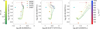 |
Fig. A.4. Same as Fig. 12 for the four galaxies identified as outliers. We shortened the object IDs in the legend for reasons of legibility, but the symbols are the same as in Fig. A.1. The model grids are those for the LMC from Allen et al. (2008), as they are a better match in metallicity for the galaxies considered. |
A.2. AGN outlier: J1152+4005
J1152+4005, the second GP in our initial sample, is the most massive galaxy (log M⋆/M⊙ = 9.94) studied in this paper, while being a compact object at rpetro ∼ 6.52 kpc. Both diagnostic diagrams (Figs. A.1 and A.2) strongly suggest that an AGN is the dominant ionisation mechanism in this object. With no notable line broadening evident in this galaxy’s spectrum, it is most reminiscent of a Seyfert 2 type nucleus.
Its faint emission lines allow no conclusive determination of the oxygen abundance, though within their large error ranges of 1.3 − 1.7 dex, the direct, emprical te and N2 methods (see Sect. 3.2) agree with a value between log(O/H) = 7.8 − 8.4, whereas the R23 method would predict an unlikely value of log(O/H) + 12 = 10.3. The comparison of the line ratios found in J1152+4005 to the LMC shock models from Allen et al. (2008) suggests that shocks may play a significant role in the ionisation of the galaxy’s ISM, but the large errors in the line ratios leave this finding somewhat unconclusive. Fig. A.4 suggests that models of strong magnetic fields B ∼ 10 μG at velocities vs > 400 km s−1 are favoured here.
A.3. SF outlier: J1514+2840
The SDSS image of J1514+2840 (Fig. A.3, bottom left panel) reveals this object is of an ambiguous nature. Its (projected) proximity to a larger galaxy suggests it may be an H II region within the galaxy in question, which by itself has no spectroscopic data published in the SDSS. As it appears to be similar to the IMPs in terms of colour and morphology, another possible classification is a ‘true’ DG which by chance is aligned with a larger background galaxy. In either case, the spectroscopic properties derived for this object are highly uncertain, as the SED is bound to include parts of both the SF object and the apparently quiescent, larger galaxy.
Even in the case of this object being a H II region, it may still be a worthwhile contender regarding the study of LyC photon loss, as the O32 value of ∼2.7 is rather large, considering the ‘contamination’ of the spectrum. Similar situations of localised ionised emission from star-forming regions or stellar clusters have previously been observed in other galaxies – to name one example, in case of Haro 11, its LyC leakage appears to be confined to one of its star-forming knots (Keenan et al. 2017).
The notion that J1514+2840 may be relevant in terms of LyC leakage is further supported by the SFH similar to that found in the IMPs, where a young and luminous metal-poor starburst occured at 10 Myr. The younger starburst episode, however, is somewhat older than the typical young population of the IMPs at 5 Myr, and its elevated metallicity of 0.4 Z⊙ may imply this stellar population is associated with the background source (Fig. A.6).
A.4. AGN outlier: J1657+4135
J1657+4135 is a true outlier in the sense that it is the only object considered in this paper where parts of the internal structure are resolved. Its SDSS image (Fig. A.3, bottom right panel) reveals it to be a spiral galaxy with at least three spiral arms, which contain blue knots of enhanced star-forming activity. Its companion in the south (SDSS J165732.76+413434.9, visible as an elongated yellow shape at the bottom of the SDSS image in Fig. A.3) is located at a similar redshift (z = 0.02869666) and their centres are separated by ∼27 kpc in projection, so a likely scenario for triggering the current star formation episode is their gravitational interaction.
While classified as a SFG in the BPT diagram (Fig. A.2), we cannot draw further conclusions concerning the presence of an AGN from He II 4686. As seen in its spectrum (Fig. A.7), the He II 4686 line is not properly detected. Noteworthy are the visibly strong absorption features, such as Ca II H&K at 3969 Å and 3934 Å, Mg I at 5177 Å, Na I D at 5892 Å, and likewise, several H I lines, particularly pronounced in the features around ∼3900 Å. However, at their given rest-frame wavelengths, the hydrogen lines show a strong, narrow emission feature superimposed on the absorption trough. This indicates that along a few lines of sight, the density of neutral gas is low, either from kinematic effects or due to a high degree of ionisation. As discussed before, star-forming regions have the means to be a driver of both these effects. The SDSS fibre, however, only covers 3″ around the galaxy’s centre, and the low value of SFR(Hα) ∼ 0.191 M⊙ yr−1 suggests no region of significantly enhanced star-formation is contained in the SDSS spectrum. We hence deem it likely that these features are related to the galaxy’s nucleus, whose activity has a strong impact on the surrounding ISM.
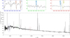 |
Fig. A.7. 3400 Å–9600 Å region of the redshift-corrected spectrum of J1657+4135, truncated in flux density f to enhance the visibility of weak spectral features (bottom row). The coloured boxes indicate the regions shown in the blow-ups in the top row and were selected to depict several features discussed in the text. The wavelengths were converted to vacuum wavelengths following Morton (1991). |
Appendix B: Emission lines
Emission line fluxes relative to Hβ, their equivalent widths and the derived Hβ extinction coefficients of the IMPs.
Same as Table B.1, but for the four galaxies identified as outliers.
All Tables
Derived properties for the galaxies in our sample as indicated in the first column.
Emission line fluxes relative to Hβ, their equivalent widths and the derived Hβ extinction coefficients of the IMPs.
All Figures
|
Fig. 1. Annotated sketch highlighting several scenarios present in an H II region around a dominant central object (DCO). Light blue arrows represent LyC photons, where an arrow ending within the extent of the H II region indicates absorption, and an arrow exceeding the region’s extent represents escape. The top left quadrant depicts the extent of H I and H II for the density- and ionisation-bounded textbook scenarios, whereas the bottom left quadrant is intended to highlight the role of a more complex gas geometry on LyC escape. The bottom right quadrant serves as a reminder that the spatial distribution of ionising sources further influences the observed LyC flux. Finally, the top right quadrant illustrates that the regions occupied by different ions vary in size, mediated by their respective ionisation potentials (an overview of the ionisation energies of a few select atoms is given in the table at the top right). |
| In the text | |
|
Fig. 2. Shirazi & Brinchmann (2012) diagram including their AGN diagnostic (green dashed line). Blue squares represent the IMPs, whereas the position of their stack is shown as a black downward-facing open triangle. Red diamonds and yellow circles mark the AGN contaminated galaxies and star-forming objects classified as outliers (see text). The grey scale density diagram represents all eligible galaxies from the SDSS DR12 with AoN > 2 in the utilised emission lines, binned in 0.02 × 0.02 dex bins for the line ratios shown. Lower contrast indicates lower bin occupancy. |
| In the text | |
|
Fig. 3. BPT diagram including the photoionisation limit from Kewley et al. (2001, red dash-dotted line) and the AGN separation line from Kauffmann et al. (2003, green dashed line). Symbols are the same as in Fig. 2. |
| In the text | |
|
Fig. 4. Distribution of EW(Hβ) (top) and EW([O III] 5007) (bottom) for the IMPs, binned in 50 Å and 500 Å bins, respectively. |
| In the text | |
|
Fig. 5. Mosaic of the SDSS gri cutouts of our final sample obtained from the SDSS SkyServer at http://skyserver.sdss.org/. Each cutout spans a region of 12.5″ × 12.5″, where north is up and east is to the left. |
| In the text | |
|
Fig. 6. Nitrogen vs. oxygen abundance, with symbols representing the same objects as in Fig. 2. The SDSS DR12 galaxies (black scatter diagram) are limited to SFGs with appropriate AoN in the line fluxes relevant for the determination of N/O and O/H with the direct method. The green dashed line is the generic scaling relation from Nicholls et al. (2017), i.e. log(N/O) = log(10−1.732+10logO/H + 2.19). |
| In the text | |
|
Fig. 7. Ionisation parameter and metallicity sensitive log(O32) = log([O III] 5007/([O III] 3727) vs. log(R23) = log(([O II] 3727 + [O III] 4959 + [O III] 5007/Hβ diagram. Symbols are the same as in Fig. 2. Additional markers were added for several low-z LyC leakers, i.e. the GPs from Izotov et al. (2016a,b, 2018a,b, green upward triangles) and low-mass galaxies from Izotov et al. (2021b, cyan left-facing triangles). Also shown are the intermediate-z LyC leakers Ion2 from de Barros et al. (2016, orange pentagram), four galaxies from Fletcher et al. (2019, dark red hexagrams, where we converted their listed [OIII] 4959,5007 values to [OIII] 5007 assuming [OIII] 5007/[OIII] 4959 = 2.98, Storey & Zeippen 2000), and AUDFs01 from Saha et al. (2020, purple right-facing triangle). The SDSS DR12 galaxies (black scatter diagram) are limited to those identified as SFGs with the BPT diagnostics from Kewley et al. (2001) and Kauffmann et al. (2003). |
| In the text | |
|
Fig. 8. Balmer decrements derived for the IMPs after accounting for foreground and internal extinction. The horizontal lines mark the expected theoretical values calculated by Storey & Hummer (1995) for ne = 100 cm−3 and te = 15 000 K, assuming Case A (dotted line) and Case B (dashed line) conditions. The * symbol signifies a likely blend of multiple lines (see text). |
| In the text | |
|
Fig. 9. SFHs of the first half of the IMPs. The top panel in each plot pair shows the SFH weighted by the stellar population’s luminosity at 4020 Å, whereas the bottom panel shows the mass-weighted SFH. Here, the black arrow marks the time where half of the galaxy’s mass was assembled, as indicated by the t1/2 inset. The bar colours correspond to the stellar metallicity as indicated by the numbers above each plot pair, in units of Z⊙. |
| In the text | |
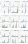 |
Fig. 10. Same as Fig. 9 for the second half of the IMPs. |
| In the text | |
|
Fig. 11. 3400 Å–9600 Å region of the stack of eighteen redshift-corrected SDSS spectra of the IMP sample, binned in 1 Å bins and truncated in flux density f to enhance the visibility of weak spectral features (bottom row). The coloured boxes indicate the regions shown in the blow-ups in the top row, centred at [FeV] 4227, He II 4686, and C IV 5808 (blue, green, and red insets, respectively). Noteworthy emission lines (both present and absent) are marked by coloured vertical lines. The SDSS wavelengths were converted to vacuum wavelengths following Morton (1991). |
| In the text | |
|
Fig. 12. Three commonly used BPT diagrams for shock diagnostics; symbols are the same as in Fig. 2. Solid lines show the shock+precursor SMC model grids from Allen et al. (2008) with their parameters (shock velocity vs and transverse magnetic field B) coloured as indicated by the colour bars. |
| In the text | |
|
Fig. 13. Spectral hardness as traced by He II 4686/Hβ vs. LyC escape fraction fesc(LyC). Blue squares represent the IMPs, whereas the position of their stack is shown as a black downward-facing open triangle. We show no error bars in fesc(LyC), as the values we infer are mere estimates from O32. The stacks from the Low-redshift Lyman Continuum Leaker Survey as provided in Marques-Chaves et al. (2022b) are shown as orange circles, and the LCEs studied in Guseva et al. (2020) as green diamonds. |
| In the text | |
|
Fig. 14. log([O III]5007/Hβ) vs. log([S II] 6717,6731/Hα) diagram including the [SII] ridge line from Wang et al. (2021, green dashed line). Symbols are the same as in Fig. 7. Left: panel highlighting the IMPs’ positions in the parameter space covered by SDSS DR12 galaxies. Right: zoom-in on the region occupied by the IMPs. |
| In the text | |
|
Fig. 15. log(O32) =log([O III] 5007/([O II] 3727) vs. Δ[S II] diagram. Symbols are the same as in Fig. 7. |
| In the text | |
|
Fig. A.1. Same as Fig. 2, highlighting three of the four outlier galaxies removed from our sample as indicated in the plot legend. |
| In the text | |
|
Fig. A.2. Same as Fig. 3, highlighting the four outlier galaxies removed from our sample as indicated in the plot legend. |
| In the text | |
|
Fig. A.3. Same as Fig. 5 for the four galaxies identified as outliers. The last panel is zoomed out by a factor of 10, i.e. spanning a region of 125″ × 125″. |
| In the text | |
|
Fig. A.4. Same as Fig. 12 for the four galaxies identified as outliers. We shortened the object IDs in the legend for reasons of legibility, but the symbols are the same as in Fig. A.1. The model grids are those for the LMC from Allen et al. (2008), as they are a better match in metallicity for the galaxies considered. |
| In the text | |
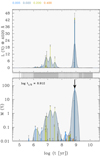 |
Fig. A.5. Same as Fig. 9 for J0225+0033. |
| In the text | |
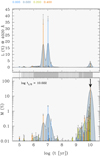 |
Fig. A.6. Same as Fig. 9 for J1514+2840. |
| In the text | |
|
Fig. A.7. 3400 Å–9600 Å region of the redshift-corrected spectrum of J1657+4135, truncated in flux density f to enhance the visibility of weak spectral features (bottom row). The coloured boxes indicate the regions shown in the blow-ups in the top row and were selected to depict several features discussed in the text. The wavelengths were converted to vacuum wavelengths following Morton (1991). |
| In the text | |
Current usage metrics show cumulative count of Article Views (full-text article views including HTML views, PDF and ePub downloads, according to the available data) and Abstracts Views on Vision4Press platform.
Data correspond to usage on the plateform after 2015. The current usage metrics is available 48-96 hours after online publication and is updated daily on week days.
Initial download of the metrics may take a while.