| Issue |
A&A
Volume 550, February 2013
|
|
|---|---|---|
| Article Number | A24 | |
| Number of page(s) | 16 | |
| Section | Stellar structure and evolution | |
| DOI | https://doi.org/10.1051/0004-6361/201220309 | |
| Published online | 21 January 2013 | |
Insights into thermonuclear supernovae from the incomplete Si-burning process
Dept. Física i Enginyeria Nuclear, Univ. Politècnica de Catalunya, Carrer Pere Serra 1-15, 08173 Sant Cugat del Vallès Spain
e-mail: eduardo.bravo@upc.edu
Received: 30 August 2012
Accepted: 24 November 2012
Type Ia supernova (SNIa) explosions synthesize a few tenths to several tenths of a solar mass, whose composition is the result of incomplete silicon burning that reaches peak temperatures of 4 GK to 5 GK. The elemental abundances are sensitive to the physical conditions in the explosion, making their measurement a promising clue to uncovering the properties of the progenitor star and of the explosion itself. Using a parameterized description of the thermodynamic history of matter undergoing incomplete silicon burning, we computed the final composition for a range of parameters wide enough to encompass current models of SNIa. Then, we searched for combinations of elemental abundances that trace the parameters values and are potentially measurable. For this purpose, we divide the present study into two epochs of SNIa, namely the optical epoch, from a few weeks to several months after the explosion, and the X-ray epoch, which refers to the time period in which the supernova remnant is young, starting one or two hundred years age and ending a thousand years after the event. During the optical epoch, the only SNIa property that can be extracted from the detection of incomplete silicon burning elements is the neutron excess of the progenitor white dwarf at thermal runaway, which can be determined through measuring the ratio of the abundance of manganese to that of titanium, chromium, or vanadium. Conversely, in the X-ray epoch, any abundance ratio built using a couple of elements from titanium, vanadium, chromium, or manganese may constrain the initial neutron excess. Furthermore, measuring the ratio of the abundances of vanadium to manganese in the X-ray might shed light on the timescale of the thermonuclear explosion.
Key words: supernovae: general / white dwarfs / nuclear reactions, nucleosynthesis, abundances
© ESO, 2013
1. Introduction
Type Ia supernovae (SNIa) are the brightest phenomena powered by nuclear reactions in the universe, releasing ~1.5 × 1051 erg that are one-third invested in overcoming the binding energy of the progenitor white dwarf (WD), and the rest in kinetic energy of the debris. The nuclear energy release takes roughly one second, implying a mean power of ~1.5 × 1044 W. These figures make SNIa prime targets for studies of nucleosynthesis in extreme conditions of density and temperature.
While there is currently little doubt that the star exploding as a SNIa is a binary WD (e.g. Nugent et al. 2011), other details of the progenitor system are uncertain; to cite a few: the nature of the companion star (either double degenerate, DD, or single degenerate, SD; Patat et al. 2007; Maoz & Mannucci 2008; Blondin et al. 2009; Simon et al. 2009; Li et al. 2011; Bloom et al. 2012; Foley et al. 2012; Maoz et al. 2012; Schaefer & Pagnotta 2012), the mass-accretion history (Chomiuk et al. 2012; Di Stefano & Kilic 2012; Shappee et al. 2012), the geometry of the flame at thermal runaway (Höflich & Stein 2002; Zingale et al. 2009), the mass of the WD at ignition (either a sub-Chandrasekhar WD, a Chandrasekhar-mass WD, or a super-Chandrasekhar one, Mazzali et al. 2007; van Kerkwijk et al. 2010; Yuan et al. 2010), or the properties of the environment within a parsec of the WD. In the SD Chandrasekhar-mass WD scenario, the structure is supported by the pressure of degenerate electrons, which can be described by a few parameters. As a consequence, only a handful of the progenitor system properties have an impact on the thermonuclear explosion, namely the central density of the WD, the initial geometry of the flame, and the chemical composition. The thermal content may also have an impact (Calder et al. 2012). Current knowledge of stellar evolution implies that the progenitor WD has to be made up mainly of carbon and oxygen, in proportions that depend on its main-sequence mass and metallicity. The metallicity has further influence on the WD structure through setting the electron mole number, Ye, which controls the number of electrons available to support the WD. It is to be expected that nature makes SNIa from a range of all the above parameters.
The workings of the thermonuclear bomb that powers a SNIa are not precisely known. Within the SD Chandrasekhar-mass WD scenario, the favored model involves an initially subsonic flame (deflagration) followed by a detonation. The release of thermonuclear energy in either burning-propagation mode is what controls the time schedule of the explosion. Thus, there is an intimate relationship between the final energy and mechanical structure of the supernova ejecta, on the one hand, and its chemical composition and profile, on the other hand. Furthermore, the chemical structure of the ejecta reflects the thermodynamic conditions in the explosion. Thus, there would be possible in principle to make an inverse analysis of the ejecta composition to uncover the details of the supernova explosion.
From the observational point of view, obtaining the chemical composition of the ejecta is not an easy task. Optical spectra depend in a complex way on the physical conditions in the ejecta days to weeks after the supernova explosion, which in turn are controlled by the energy deposition from radioactive nuclei, mainly 56Ni and its decay product 56Co. However, recently there have been advances that allow performing detailed tomographies of a few well-studied SNIa (Stehle et al. 2005a; Altavilla et al. 2007; Mazzali et al. 2008; Tanaka et al. 2011). It is to be expected that the set of SNIa for which a detailed chemical composition of the ejecta is available will increase steadily in the next several years.
An alternative way to gain knowledge about the chemical structure of the ejecta is through studying young supernova remnants (Badenes 2010). Badenes et al. (2008) studied the relationship between X-ray spectral features due to Mn and Cr in young SNIa remnants and the metallicity of the WD progenitor, which allowed them to conclude that the metallicity of the progenitor of Tycho’s supernova is supersolar. The same technique has been since applied to other suspected SNIa remnants to determine their progenitors’ metallicity.
The picture of SNIa ejecta drawn from observations has converged to a layered chemical structure, although with exceptions and peculiarities (e.g. Folatelli et al. 2012). In the center, there is a volume filled with relatively neutron-rich iron-group elements (Höflich et al. 2004), thought to arise from matter heated to more than ~5.5 billion degrees, which achieved nuclear statistical equilibrium (NSE) and thereafter was neutronized efficiently by electron captures. This neutronization clears the center of the main radioactive product of SNIa, 56Ni. Above the central core, there is a volume made of iron group elements that achieved NSE at a density low enough to experience a negligible amount of neutronization. This volume is mainly composed of 56Ni. Outwards from this region, there is a volume made of the products of incomplete silicon burning (hereafter, Si-b), covering a wide range in atomic number, from silicon to iron. Finally, close to the surface of the ejecta, there is a tiny region made of unburned fuel and material that has been processed no further than oxygen burning. The details of the layered structure vary from object to object, and not all the observations point to the same degree of chemical stratification. Some objects seem to have experienced a thorough mixing of the two outer layers, unburned and Si-b matter (Stehle et al. 2005b), although there is evidence that iron-group nuclei and the products of Si-b have clearly different physical histories (Rakowski et al. 2006).
Although the masses of the different layers of SNIa ejecta are thought to vary from object to object, it can be said that NSE matter should amount from 0.2 to 0.8 M⊙, whereas intermediate-mass elements, mainly made as a result of Si-b, cover more or less the same range of masses (Mazzali et al. 2007). In principle, the study of both regimes therefore has the capability of providing interesting clues to the nature of the explosion. However, whereas the abundances of NSE matter are influenced by the amount of electron captures achieved in the first phases of the explosion, the composition resulting from Si-b only depends on the initial composition of the supernova progenitor and on the dynamics of the explosion.
The purpose of the present work is to elucidate the dependence of the chemical composition arising from Si-b on the progenitor properties (metallicity and chemical composition of the exploding WD) and on the explosion dynamics (expansion timescale and combustion wave velocity). We note that, although incomplete silicon burning has been studied in depth in quite a few works (e.g. Bodansky et al. 1968; Woosley et al. 1973; Hix & Thielemann 1996, 1999; Meyer et al. 1996, 1998), none of them have looked at the final chemical composition for tracers of the parameters governing this nucleosynthetic process. We use a model of the thermodynamic evolution of matter undergoing Si-b, which we explain and justify in the next section. Thereafter, we focus on abundance ratios of Si-b products, which allows us to avoid the problem posed by the dependence of the absolute abundances on the total energy of the supernova. We split the results into two groups of abundance ratios: on the one hand, those that might create a detectable signature in the optical display of the supernova, encompassing between a few days and a few months after the explosion, which we term the optical phase or the optical epoch; and on the other hand, those that would apply to supernova remnants several hundred years after the event, which we term the X-ray phase or the X-ray epoch, because abundance measurements in this phase are usually obtained from X-ray spectra. We also refer to the first second of the explosion as the nucleosynthetic epoch, since it is then when the nuclear fluxes are able to modify the final chemical composition, apart from radioactive disintegrations.
2. Numerical method
We performed the nucleosynthetic calculations described in this paper by solving the nuclear kinetics equations with the code CRANK described in Bravo & Martínez-Pinedo (2012). For completeness, we summarize here its main features. CRANK integrates the temporal evolution of the abundances in a nuclear network for given thermal and structural (density) time profile, and for initial composition. The inputs to CRANK are the nuclear data and the thermodynamic trajectories, as a function of time. The thermodynamic trajectories, in turn, can be the result of a hydrodynamic calculation of an explosive event, in which case CRANK provides the final chemical profile of the ejecta after computing the nucleosynthesis of each mass shell independently, without accounting for chemical diffusion. Alternatively, CRANK can compute the nucleosynthesis in a single homogeneous region using an arbitrary thermodynamic trajectory. In the present work, we use CRANK in the latter way.
The nuclear evolutionary equations (see e.g. Rauscher et al. 2002) follow the time evolution of the molar fraction of each nucleus until the temperature falls below 108 K, after which time the chemical composition is no longer substantially modified, with the exception of radioactive disintegrations. The integration of the nuclear network follows the implicit iterative method of Wagoner with adaptive time steps. The iterative procedure ends when the relative variation in the molar abundances is smaller than 10-6, taking only those nuclei with molar abundance Y > 10-14 mol g-1 into account. The number of iterations is limited to 7, and if this limit is reached a new iteration procedure with a reduced time step is started from the abundances at the last successful integration. In case the relative variation in the abundance of any nuclei with Y > 10-14 mol g-1 is greater than a prescribed tolerance, the iteration procedure is restarted from the last successful integration, but with a smaller time step. The sum of mass fractions is checked upon completion of each iteration procedure. If that sum differs from one more than 10-8, the iteration procedure needs to be restarted with a smaller time step.
The network is adaptive, in the sense that its size (nuclei and reactions linking them) varies during the computation in order to improve its performance. A nucleus enters the calculation only if either it has an appreciable abundance (Y > 10-24 mol g-1) or it can be reached from any of the abundant nuclei by any one of the reactions included in the network. Light particles (neutrons, protons, and alphas) are the exception to the rule, because they are always included in the network. A reaction rate is included in the network only if the predicted change it induces on a molar abundance in the next time step is larger than a threshold, fixed at 10-20 mol g-1 (see Rauscher et al. 2002, for a similar method).
The nuclear network consists of a maximum of 722 nuclei, from free nucleons up to 101In, linked by three fusion reactions: 3α, 12C+12C, and 16O+16O, electron and positron captures, β− and β + decays, and 12 strong interactions per each nucleus with Z ≥ 6, involving neutrons, protons, alphas, and γ. We take the necessary nuclear data from Salpeter & van Horn (1969); Itoh et al. (1979); Fuller et al. (1982); Martínez-Pinedo et al. (2000); Cyburt et al. (2010).
3. Modeling the physical conditions in incomplete silicon burning in SNIa
Explosive nucleosynthesis studies can be divided into two broad categories, namely those that follow the thermodynamic trajectories computed from hydrodynamic models of the exploding object (e.g. Thielemann et al. 1986; Maeda et al. 2010), and those that adopt a simplified parameterized description of the time dependence of the relevant thermodynamic variables (Woosley et al. 1973; Meyer et al. 1998; Hix & Thielemann 1999). The former ones are more adequate for determining the chemical composition of the ejecta of a particular supernova (or whatever exploding object) model. The second ones are suitable for studies aiming at elucidating nucleosynthetic properties expected to be shared by a general class of explosion models. Here, we chose this second approach because we are interested in just one nucleosynthetic process among all that are at work in SNIa.
As is customary in parameterized studies of high-temperature explosive nucleosynthesis (op cit), we model the temporal evolution of the mass zone undergoing Si-b as a fast heating followed by adiabatic expansion and cooling. The temperature as a function of time is given by ![\begin{equation} \label{eqT} T_9 = \left\{ \begin{array} {r@{:\quad}l} T_{9,0}+\left(T_{9, {\rm peak}}-T_{9,0}\right)t/\tau_{{\rm rise}} & 0\le t\le \tau_{{\rm rise}} \\ T_{9, {\rm peak}}\exp\left[-\left(t-\tau_{{\rm rise}}\right)/\tau\right] & \tau_{{\rm rise}} < t, \\ \end{array} \right. \end{equation}](/articles/aa/full_html/2013/02/aa20309-12/aa20309-12-eq23.png) (1)where t is time, T9 is the temperature in units of 109 K, and the rest of the quantities are model parameters, namely τrise is the time to reach the maximal temperature, T9,peak, starting from an initial value, T9,0, and τ is the expansion timescale. In some studies, the expansion timescale has been taken as the free fall timescale,
(1)where t is time, T9 is the temperature in units of 109 K, and the rest of the quantities are model parameters, namely τrise is the time to reach the maximal temperature, T9,peak, starting from an initial value, T9,0, and τ is the expansion timescale. In some studies, the expansion timescale has been taken as the free fall timescale,  ; however, we prefer to keep it as a free parameter in the present work. The initial temperature, T9,0 is irrelevant as long as it is low enough compared to the peak temperature. We fixed its value at T9,0 = 1 in all the numerical experiments.
The density is given by ![\begin{equation} \label{eqro} \rho_7 = \left\{ \begin{array} {r@{:\quad}l} \rho_{7,0}+\left(\rho_{7, {\rm peak}}-\rho_{7,0}\right)t/\tau_{{\rm rise}} & 0\le t\le \tau_{{\rm rise}} \\ \rho_{7, {\rm peak}}\exp\left[-3\left(t-\tau_{{\rm rise}}\right)/\tau\right] & \tau_{{\rm rise}} < t, \\ \end{array} \right. \end{equation}](/articles/aa/full_html/2013/02/aa20309-12/aa20309-12-eq33.png) (2)where ρ7 is the density in units of 107 g cm-3, ρ7,peak is the maximal density, and ρ7,0 is the initial density, whose value is not influential in the present results and is fixed in the calculations at ρ7,0 = 0.3ρ7,peak. The factor three in the exponential in Eq. (2) accounts for the ρ ∝ T3 dependence, appropriate to describing the isentropic evolution of a radiation-dominated gas (Hix & Thielemann 1999).
(2)where ρ7 is the density in units of 107 g cm-3, ρ7,peak is the maximal density, and ρ7,0 is the initial density, whose value is not influential in the present results and is fixed in the calculations at ρ7,0 = 0.3ρ7,peak. The factor three in the exponential in Eq. (2) accounts for the ρ ∝ T3 dependence, appropriate to describing the isentropic evolution of a radiation-dominated gas (Hix & Thielemann 1999).
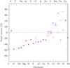 |
Fig. 1 Error in the elemental yields obtained with Eqs. (1) and (2) relative to those for the same element obtained with the thermodynamic trajectories provided by a hydrodynamic code for a SNIa model (see text for further details). Large open (red) circles give the errors belonging to a time of one day after the explosion, when the abundances of many iron-group elements are still dominated by radioactive isotopes. Small filled (blue) circles give the errors belonging to a time one hundred years after the explosion. Points belonging to some interesting couples of elements are highlighted by a small ellipse around them. For this comparison, we have only considered the layers with peak temperatures between 4.3 and 5.2 GK. |
Although adiabatic expansion is a common assumption, matter heated to temperatures high enough to achieve partial or total nuclear statistical equilibrium, T ≳ 4 × 10⁹ K, may go off the isentropic thermodynamic path because of the continuous adjustment of the chemical composition as temperature declines, which releases nuclear energy. The degree to which Eqs. (1) and (2) provide a faithful representation of the nucleosynthesis in SNIa layers undergoing Si-b can be tested, for any given SNIa model, by computing the chemical composition from these equations with parameters fitted to the thermodynamic trajectories provided by the hydrodynamic code, then comparing it to the chemical composition obtained with the original thermodynamic trajectories.
Figure 1 compares the yields obtained for the same elements with the two thermodynamic time evolutions described in the previous paragraph, for the SNIa model DDTc described in Badenes et al. (2005) and Bravo & Martínez-Pinedo (2012) and used hereafter as a reference model. As can be deduced from the figure, the errors in the abundances of elements from silicon to niquel related to the use of Eqs. (1) and (2) range from −40% to +70%. Most important, taking ratios of the yields of different elements, the errors can be made very tiny. For instance, the errors of the yields of the elements belonging to the first quasi-statistical equilibrium (QSE) group, i.e. those between silicon and scandium, are all very similar, implying that the ratio of the yields obtained with Eqs. (1) and (2) are a very good representation of the ratios belonging to the full thermodynamic trajectories provided by the supernova model. The errors of the elements belonging to the second QSE group, i.e. those between titanium and zinc, are much more heterogeneous. However, couples of elements can be identified in Fig. 1 whose yields are affected by a very similar error, hence for whom the yield ratios are predicted well by using Eqs. (1) and (2). An example is the couple formed by titanium and vanadium, at both one day and one hundred years after the explosion. Another example is the couple formed by chromium and manganese at one hundred years after the explosion.
We also tried fitting the thermodynamic histories of supernova layers with more complicated algebraic functions, but we obtained no improvements over the single exponential dependence on the adiabatic expansion timescale.
3.1. Parameters ranges
With the temporal evolution of temperature and density given by Eqs. (1) and (2), the full set of parameters that controls the final chemical composition of mass layers undergoing incomplete Si-b are the peak temperature T9,peak, the peak density ρ7,peak, the expansion timescale τ, the temperature rise timescale τrise, the initial mass fraction of 12C, X(12C), and the initial mass fraction of 22Ne, X(22Ne). The last two quantities provide a convenient parameterization of the chemical composition of the WD at runaway. In this work, we simply assume that the only species initially present in the WD are 12C, 16O, and 22Ne. The initial mass fraction of oxygen is thus  (3)and the initial neutron excess is
  (4)In turn, the initial neutron excess is related to the metallicity of the supernova progenitor, Z, through η ≈ 0.101Z (Timmes et al. 2003), which leads to, Z ≈ X(22Ne)/1.111.
In the following, we discuss the relevant ranges of the parameters to explore.
3.1.1. Peak temperature
In our reference model, DDTc, as well as in most SNIa models (e.g. Woosley et al. 1973; Hix & Thielemann 1999; Maeda et al. 2010), incomplete Si-b is achieved at densities slightly in excess of 107 g cm-3 (see Fig. 1 in Bravo & Martínez-Pinedo 2012). At these densities, to achieve the QSE of the iron group and of the silicon group, the peak temperature has to exceed ~4 × 10⁹ K. On the other hand, to avoid reaching full NSE the temperature should remain well below ~5.5 × 10⁹ K (Woosley et al. 1973). As we demonstrate later, the most promising targets of the present study are the lightest elements of the iron-group, from titanium to manganese. As can be seen in Table 2 of Bravo & Martínez-Pinedo (2012), the bulk of these elements originates in SNIa in layers attaining temperatures in the range from 4.2 × 10⁹ K to 5.2 × 10⁹ K, with the exception of manganese, which has a sizeable contribution from layers reaching NSE. For the purposes of the present study, we define the range of peak temperatures able to provide incomplete Si-b such as that between 4.3−5.2 × 10⁹ K.
Figure 2 shows the evolution of the nuclear species computed with T9,peak = 4.8, ρ7,peak = 2.2, τ = 0.29 s, τrise = 10-9 s, X(12C) = 0.5, and X(22Ne) = 0.01. For this set of parameters, and in spite of the high temperature attained, there is no appreciable change in the chemical composition before t = τrise. Carbon is exhausted in a time of a few tens of ns and oxygen burns at less than 10 μs, whereas the isotopes belonging to the silicon QSE-group achieve stable proportions after ~0.1 ms. It can be seen that the species of the iron QSE-group steadily increase in abundance after ~1 ms and until the expansion cools matter below ~4 × 10⁹ K. After this point, two different trends in the isotopes belonging to the iron QSE-group can be discerned. On the one hand, 56Ni is the only species that continues growing in abundance. On the other hand, the mass fractions of the rest of the most abundant components of the iron QSE-group, rich in neutrons, decrease owing to recombination with excess free protons and alphas, adapting their abundances to equilibrium at the decreasing temperatures, while they remain above T ≳ 3 × 10⁹ K (Hix & Thielemann 1999). This recombination causes a drop in the abundance of 4He after ~0.01 s, which is clearly visible in the plot.
It is notable that the final mass fractions of 55Co (55Mn after a few years of radioactive disintegration) and 52Fe (grandparent of 52Cr) are among the largest from the iron QSE-group. But for 54Fe and 56Ni, they are the most abundant species with η ≠ 0 and with η = 0, respectively.
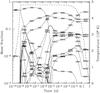 |
Fig. 2 Evolution of the chemical composition for a reference set of parameters, namely Tpeak = 4.8 109 K, τrise = 10-9 s, τ = 0.29 s, X(12C) = 0.5, X(22Ne) = 0.01. The dashed line is the temperature in 109 K. |
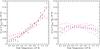 |
Fig. 3 Distribution of maximal temperatures in the incomplete Si-burning region obtained from a suite of SNIa models. Left: one-dimensional delayed detonation models DDTc (red crosses, Badenes et al. 2005) and DDTf (red solid squares), a sub-Chandrasekhar model (blue stars) from Bravo et al. (2011, fourth row in their Table 2), and three-dimensional delayed detonation model TURB7 from Bravo et al. (2009, red empty squares,). The solid line is a fit to the data given by, |
3.1.2. Distribution function of peak temperatures.
In any model of SNIa, matter attains a wide range of peak temperatures. As the burning front moves through layers of decreasing density, its peak temperature drops. Matter experiencing Si-b is not subject to just a single peak temperature but to a sequence of them. Figure 3 shows the distribution of peak temperatures in a suite of SNIa models of different flavors. The distribution function of peak temperatures in these models can be described by either an approximately power-law dependence on T9,peak, which we fit with  , or as independent of T9,peak. Aside from the models shown in these figures, model O-DDT in Maeda et al. (2010) follows a dependence on T9,peak that is similar to the proposed power law, at least qualitatively, whereas those of models W7 and C-DEF (op cit) are described better as independent of T9,peak.
In the following, we use these two representative distribution functions of the peak temperatures to estimate the mass of the different elements created by given combinations of the parameters of Si-b evolution, and we analyze the impact of the peak-temperature distribution function on the results. If this impact were sizeable, observations might provide insight into the distribution function of peak temperatures in SNIa. If, on the other hand, its impact is negligible, the results will be independent of the assumed distribution function.
3.1.3. Peak density
Peak density in Si-b depends on the peak temperature, both quantities being correlated with entropy. Meyer et al. (1998) introduced a quantity proportional to the entropy per nucleon in photons, 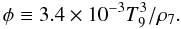 (5)Given the thermodynamic history described by Eqs. (1) and (2), φ remains constant.
For model DDTc, in the region undergoing incomplete Si-b the peak density, ρ7,peak can be approximated as a function of the peak temperature by the relationship 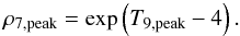 (6)
(6)
Using this equation, φ ranges from 0.15 to 0.2, which are much lower values than investigated in Meyer et al. (1998). In SNIa, the peak temperature and density are the result of the thermodynamic conditions in matter that is either shocked in a detonation wave (delayed-detonation models) or burnt subsonically (deflagration models). Khokhlov (1988) provides the peak temperature and density for Chapman-Jouguet deflagration and detonation waves, which differ from Eq. (6) by at most 22% in the temperature and density ranges of Si-b.
To reduce the number of free parameters, we use Eq. (6) in the calculations reported in the present work. It is therefore necessary to evaluate the degree of uncertainty derived from this relationship. This is done in Fig. 4, where we represent the ratio from manganese to chromium at the X-ray epoch, for peak densities given by either Eq. (6), a factor of two higher or a factor of two lower. It is clearly seen that the precise value of the peak density is irrelevant to the mass ratio of these elements. The points belonging to the different peak densities used are nearly indistinguishable in the plot, except at the highest neutron excess and the lowest temperature. These last points belong to the highest entropies studied in the present work. It is interesting to note that Meyer et al. (1998) explored even highest entropies and neutron excesses.
 |
Fig. 4 Final mass fraction ratio Mn/Cr, at a time of 100 yrs after the explosion, as a function of peak temperature in incomplete Si-b for different maximal densities (point type) and initial neutron excesses (color online). The maximal densities are given by either Eq. (6) (filled circles), or by a factor of two higher (triangles), or lower (crosses) than Eq. (6). The initial neutron excesses are η = 2.27 × 10⁻⁴ (red), 9.09 × 10⁻⁴ (blue), and 6.82 10-3 (black), increasing from bottom to top. |
3.1.4. Rise time
Most, if not all, nucleosynthetic studies of the explosive incomplete Si-b process compute the nuclear flows starting from the peak temperature and the initial fuel composition. Woosley et al. (1973) argue that this is justified when the rise time, i.e. the time taken to dump the energy needed to raise its temperature to its peak value into the mass zone, is much shorter than the expansion timescale, τrise ≪ τ. In SNIa models, the energy dumped into a zone until it reaches its peak temperature can either be due to a compressional heating related to the passage of the shock front at the leading edge of a detonation wave or it is a combination of thermal diffusion and energy released by nuclear reactions in a deflagration wave. The rise time associated with each one of these burning waves is very different.
Figure 5 shows a comparison of both rise times as a function of density, together with the hydrodynamic timescale. The thermal structure of a laminar flame (deflagration) is determined by heat diffusion from hot ashes to cool fuel at low temperature and by the release of heat by nuclear reactions at high temperature. The transition between both regimes takes place at a critical temperature, Tcrit, that depends on density. The deflagrative timescale in Fig. 5 has been estimated as the nuclear timescale at Tcrit. For simplicity, both Tcrit and the nuclear timescale were computed, accounting only for the dominant reaction rate, i.e. the fusion of two 12C nuclei.
Triggering of ignition in a supersonic combustion wave (detonation) is due to an initial temperature jump in a length scale of a few mean free paths, in a shock front. Later on, the heat released by thermonuclear reactions determines the thermal profile. Thus, the detonation timescale can be estimated as the nuclear timescale at the shock temperature, Tshock. For the calculations shown in Fig. 5, the shock temperature was calculated by solving the Hugoniot jump conditions using the velocities of Chapman-Jouguet detonations given in Khokhlov (1988).
The detonation rise time is the shortest one by orders of magnitude, whereas the deflagration rise time lies between the detonation rise time and the hydrodynamic timescale. An alternative way of estimating the timescale of a deflagration is as the ratio between the flame width and velocity. Using the flame properties reported in Timmes & Woosley (1992), the deflagration timescale goes into the range 9 × 10⁻³−10-4 s for densities between 107 and 5 × 10⁷ g cm-3. Although these timescales are about one order of magnitude longer than the ones in Fig. 5, the qualitative conclusions remain the same.
In view of the large difference between both rise times and the hydrodynamic timescale, it is to be expected that the precise value of τrise will be unimportant for the nucleosynthesis. Notwithstanding this expectation, we have explored the nucleosynthesis resulting from different rise times ranging from 10-9 s to 0.2 s, in search for possible, although improbable, tracers of the type of burning wave responsible for incomplete Si-b in SNIa.
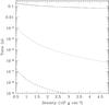 |
Fig. 5 Comparison of relevant timescales as a function of the initial density. Solid line: expansion timescale, computed as the free-fall or hydrodynamic timescale, |

Figure 6 shows the evolution of nuclear species for conditions similar to those in Fig. 2 apart from the rise time. In the left hand panel of this figure, the rise time has been set to 10-5 s to illustrate the case of a deflagration wave, whereas Fig. 2 is more representative of a detonation wave. In spite of some differences in the evolution of the chemical abundances, as for instance in the extent of burning before T9,peak, the final mass fractions in both figures are identical, in line with the predictions of Woosley et al. (1973). Moreover, the same conclusion applies to a calculation with a rise time, τrise = 0.1 s, comparable to the expansion timescale (right panel in Fig. 6).
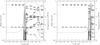 |
Fig. 6 Evolution of the chemical composition for a rise time to the maximal temperature different from that in the reference set of parameters (Fig. 2). Left: slower rise to the peak temperature, τrise = 10-5 s. Right: rise time comparable to the expansion timescale, τrise = 0.1 s. |
3.1.5. Expansion timescale
In SNIa, the expansion timescale is bounded to be longer than the WD sound-crossing time, τ ≳ tsound = RWD/vsound ≈ 0.1−0.2 s, which is similar to the free-fall timescale at the densities of interest to incomplete Si-b. In the present work, we explore expansion timescales in the range 0.1−0.9 s.
The left hand panel of Fig. 7 shows the evolution of the chemical composition for an expansion timescale τ = 0.72 s, i.e. slower than the one in Fig. 2, τ = 0.29 s, while the rest of parameters remain unchanged. As could be expected, the differences only appear in the final phase of the evolution, as can be seen in the temperature curve and in the leveling out of the abundances when all the species leave QSE. Interestingly, a longer expansion timescale favors synthesis of a larger quantity of 56Ni at the expense of 28Si and 32S, but the rest of the species with X > 0.001 is hardly affected at all.
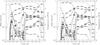 |
Fig. 7 Evolution of the chemical composition for different expansion timescales and initial carbon abundances than in the reference set of parameters (Fig. 2). Left: slower expansion timescale, τ = 0.72 s. Right: smaller carbon abundance, X(12C) = 0.3. |
3.1.6. Initial carbon abundance
Domínguez et al. (2001) accurately computed the evolution of stars in the range 1.5−7 M⊙ from main sequence to the formation of a WD, starting from different metallicities. According to their results, the carbon mass fraction in the WD lies in the range 0.37−0.55. We therefore explore a slightly wider range from X(12C) = 0.3 to X(12C) = 0.7.
The right hand panel of Fig. 7 shows the evolution of the chemical composition for initial abundances X(12C) = 0.3 and X(16O) = 0.69. Comparison with Fig. 2, in which X(12C) = 0.5 and X(16O) = 0.49, reveals that the initial carbon abundance has no influence on the final nucleosynthesis of the most abundant elements. Once oxygen is exhausted, the evolution in both figures is identical.
3.1.7. Progenitor metallicity
Type Ia supernovae are detected in host galaxies with a wide range of metallicities (e.g. Z ≈ 0.1−2.5 Z⊙ in D’Andrea et al. 2011), with apparent preference for hosts with Z > Z⊙. The low end of the metallicity range might reache Z ≈ 0.04 Z⊙ according to the preliminary results in Rigault et al. (2011). Here, we present results of incomplete Si-b for initial 22Ne mass fractions between 2.5 × 10⁻⁴ and 7.5 × 10⁻², i.e. Z ≈ 0.02−5 Z⊙ for a solar metallicity Z⊙ ≈ 0.012−0.014 (Lodders 2003; Asplund et al. 2006).
Figure 8 shows the evolution of the chemical composition starting from a neutron excess 7.5 times longer than in Fig. 2. Comparing these two figures, the impact of the initial neutron excess on the final abundances is evident. In Fig. 8, the initial amount of 22Ne disappears as soon as carbon is consumed. The role of 22Ne as the main neutron-excess holder is later played by 34S in oxygen burning, and by 54Fe and 55Co in silicon burning and during freeze-out.
3.2. Summary of model parameters
To summarize, four free parameters remain for which we try to find tracers from the nucleosynthesis of incomplete Si-b, namely the temperature rise time, the expansion timescale, the initial carbon abundance, and the progenitor metallicity, Z ≈ X(22Ne)/1.11, see Table 1. The initial values of temperature and density, T9,0 and ρ7,0, are fixed, and the peak density is linked to the peak temperature through Eq. (6). Finally, the peak temperature is another parameter that is varied in the different nucleosynthetic calculations, but such results are integrated using the distribution function of peak temperatures. To be precise, in the following when we present the results for a given set of parameters [τrise, τ, X(12C), and Z], the mass fraction of each element is given by 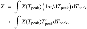 (7)with
  , and either n = 11 or n = 0 (Fig. 3).
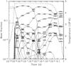 |
Fig. 8 Evolution of the chemical composition for an initial neutron excess higher than in the reference set of parameters (Fig. 2), X(22Ne) = 0.075. |
4. Tracers of the progenitor metallicity: X-ray epoch
Since isotopic abundances cannot be measured in supernova ejecta, it is convenient to know what isotopes are the main contributors to the abundances of elements made in incomplete Si-b, in the X-ray as well as in the optical epochs. This information is given in Table 2. When focusing on the X-ray phase, all the radioactivities that synthesize sizeable quantities of elements from scandium to iron cease a long time before forming a supernova remnant, so their elemental abundances remain constant at this epoch.
The only pairs of elements whose mass ratio in the X-ray epoch correlates strongly with progenitor metallicity are manganese vs. chromium, manganese vs. titanium, and vanadium vs. titanium. We discuss them next, starting with the ratio of manganese to chromium, which was originally proposed by Badenes et al. (2008) as a metallicity tracer.
Parent species of Si-b elements at the optical and X-ray epochs.
4.1. Ratio of manganese to chromium
Figure 9 shows the ratio of the abundances, either total masses or mass fractions, of manganese to chromium (Mn/Cr) in the X-ray epoch, averaged by applying Eq. (7), as a function of the initial neutron excess. The insensitivity of the Mn/Cr ratio to the temperature rise time and to the initial carbon abundance is remarkable, as well as to the distribution function of peak temperatures. At any given neutron excess, the final Mn/Cr ratio varies by less than a factor of two for the whole range of the rest of parameters, whereas the Mn/Cr ratio as a function of η varies as much as a factor of 80. Furthermore, manganese and chromium are one of the element pairs whose ratio is determined better with the simplified thermodynamic evolution provided by Eqs. (1) and (2) (see Fig. 1). Thus, the Mn/Cr ratio stands out as a robust tracer of the initial neutron excess at WD runaway. The Mn/Cr ratio can be fit as a function of η by a power law2 (Fig. 9), 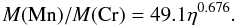 (8)The results presented here are complementary to the work of Badenes et al. (2008), where the Mn/Cr ratio is computed for a series of SNIa models. We find a similar power-law exponent as the one reported in that work, 0.676 vs. 0.65, and the new power-law fit stays within a factor of two from the one in Badenes et al. (2008).
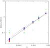 |
Fig. 9 Averaged final mass fraction ratio Mn/Cr as a function of the initial neutron excess. The average mass fractions are drawn either from the fit to the distribution of maximum temperatures given in the left panel of Fig. 3 (red circles) or from a uniform distribution function representative of the models shown in the right panel of the same figure (blue crosses). In both cases, the results are shown for different τrise in the range 10-9−0.2 s, τ in the range 0.10−0.90 s, and X(12C) in the range 0.3−0.7. The solid line is a fit given by, M(Mn)/M(Cr) = 49.1η0.676. The dashed line shows the relationship expected from an analytic model, Eq. (17). Green stars give the mass fraction ratio Mn/Cr for high-entropy conditions (see text for details). |
The robustness of the Mn/Cr ratio as a metallicity tracer is enhanced by its relative insensitivity to the peak temperature (Fig. 4). As a result, the Mn/Cr ratio is insensitive to the degree of mixing the nucleosynthetic yields for the supernova layers undergoing incomplete Si-b.
One can wonder if the Mn/Cr ratio can be used as a metallicity tracer for core-collapse supernovae. The answer is no, as long as layers experiencing Si-b in core collapse supernovae evolve through a much higher isoentropic than in SNIa. We show in Fig. 9 the results of the Mn/Cr mass ratio as a function of η when the parameter φ defined in Eq. (5) takes the value φ = 6.8, which is appropriate for core collapse supernovae (Meyer et al. 1996), while τ varies in the range 0.29−0.87 s, and the range of X(12C) is 0.3−0.7. It can be deduced from this figure that the tight relationship between the abundances of Mn and Cr and the metallicity is a result of a low entropy evolution that cannot be extrapolated to core-collapse conditions.
4.1.1. Understanding the link between neutron excess and the final ratio of manganese to chromium
It is instructive to try to understand the origin of the tight dependence of the Mn/Cr ratio in the X-ray epoch on the initial neutron excess. For this purpose, it is necessary to tell the story of the synthesis of their parent species, 55Co and 52Fe (see Table 2).
At the peak temperatures studied here, both 55Co and 52Fe attain abundances in statistical equilibrium with the iron QSE-group. As temperature drops, both nuclei evolve to maintain this equilibrium, which is broken when T < 3 × 10⁹ K (Hix & Thielemann 1999). The left hand panel of Fig. 10 shows the evolution of the abundances of 55Co and 52Fe during expansion and cooling for six different sets of parameters, given in Table 3. It can be seen that the abundance of 55Co levels off at T ≃ 2.5 × 10⁹ K, whereas that of 52Fe stabilizes even earlier, at T ≃ 3.5 × 10⁹ K. The highest differences between the curves belonging to 55Co are found for the extremes metallicities tested: the bottom solid curve, X(22Ne) = 2.5 × 10⁻⁴, and the top solid curve, X(22Ne) = 0.075. The abundance of 55Co remains in equilibrium with theirs neighbors in the iron QSE-group until T ≃ 2 × 10⁹ K, as can be seen in the right hand panel of Fig. 10. In this figure, the molar fluxes of the main reactions linking 55Co with other members of the iron QSE-group are plotted, where the most important are 54Fe + p ⇆ 55Co + γ and 56Ni + γ ⇆ 55Co + p. The flux rate of the proton capture on 55Co begins to depart from the rate of the (γ,p) reaction on 56Ni just after T ≃ 2.8 × 10⁹ K. However, the net rate of destruction of 55Co is always at least an order of magnitude lower than the rate of each of the reactions 54Fe + p ⇆ 55Co + γ, thus ensuring that equilibrium is maintained in the temperature range shown in Fig. 10. Assuming that the abundances within the iron QSE-group remain in equilibrium allows us to formulate a simple model for the ratio of the final (before radioactive disintegrations) mass fractions of 55Co to 52Fe, X(55Co)/X(52Fe).
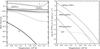 |
Fig. 10 Nuclear evolution as a function of temperature during expansion and cooling. Left: evolution of the mass fractions of 55Co (solid lines), 52Fe (dashed lines), and α (dot-dashed lines), for six different sets of parameters, as given in Table 3. The dotted lines show the quantity f, defined in Eq. (16). Right: evolution of the molar fluxes of the main reactions contributing to the abundance of 55Co for the same set of parameters as in Fig. 2. Reactions building 55Co are drawn as solid lines, reactions destroying it are drawn as dashed lines, and the absolute value of the net rate of dY(55Co)/dt is drawn as a dotted line. Upper curves are for the reactions 54Fe + p ⇆ 55Co + γ, in which both line types are nearly indistinguishable. The middle curves are for the reactions 56Ni + γ ⇆ 55Co + p. Finally, the bottom curves are for the reactions 55Fe + p ⇆ 55Co + n. |
We begin by assuming that the initial neutron excess in the matter subject to incomplete Si-b is stored in the species 54Fe and 55Co at the end of the nucleosynthetic epoch, which can be justified in light of Figs. 2 and Figs. 6−8. Then, using Eq. (4), one can write 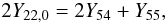 (9)where Y22,0 = X(22Ne)/22 is the initial molar fraction of 22Ne and for simplicity, we write the molar fraction of species AZ as YA, in mol/g. Another relationship between the abundances of 54Fe and 55Co can be derived from the assumption of equilibrium of the forward and backward (p,γ) reactions linking both nuclei, and the ones linking 55Co with 56Ni,
 ![\begin{equation} \label{eqequil1} Y_{55} = \left( Y_{54} Y_{56} \frac{r_{54\mbox{p}\gamma}\lambda_{56\gamma\mbox{p}}} {r_{55\mbox{p}\gamma}\lambda_{55\gamma\mbox{p}}} \right)^{1/2} = \left[ Y_{54} Y_{56} \frac{C(^{55}{Co})^2}{C(^{54}{Fe}) C(^{56}{Ni})} \right]^{1/2}, \end{equation}](/articles/aa/full_html/2013/02/aa20309-12/aa20309-12-eq165.png) (10)where r54pγ is the rate of radiative proton capture on 54Fe, λ56γp is the rate of photodisintegration of 56Ni through the proton channel, and so on. The last equality is a result of the assumption of global equilibrium within the iron QSE-group, where the quantity C(AZ) is defined by (see, e.g. Hix & Thielemann 1996),
(10)where r54pγ is the rate of radiative proton capture on 54Fe, λ56γp is the rate of photodisintegration of 56Ni through the proton channel, and so on. The last equality is a result of the assumption of global equilibrium within the iron QSE-group, where the quantity C(AZ) is defined by (see, e.g. Hix & Thielemann 1996), ![\begin{equation} C(^AZ) = \frac{G(^AZ)}{2^A} \left(\frac{\rho N_{\mbox{A}}}{\theta}\right)^{A-1} A^{3/2} \exp \left[\frac{B(^AZ)}{kT}\right], \end{equation}](/articles/aa/full_html/2013/02/aa20309-12/aa20309-12-eq169.png) (11)where G(AZ) is the partition function, B(ZA) the nuclear binding energy, NA Avogadro’s number, k Boltzmann’s constant, and
(11)where G(AZ) is the partition function, B(ZA) the nuclear binding energy, NA Avogadro’s number, k Boltzmann’s constant, and  .
.
Solving Eq. (10) for Y54 and substituting in Eq. (9) gives the following relationship between the final abundance of 55Co and the initial abundance of 22Ne, 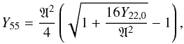 (12)where A has been defined as
 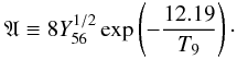 (13)Equation (12) sets the functional dependence of Y55 on X(22Ne) (or η): for X(22Ne) ≪ A2 it leads to Y55 ∝ X(22Ne), whereas for X(22Ne) ≫ A2 the result is Y55 ∝ X(22Ne)1/2. Since A ~ 0.011 when global QSE breaks down (T9 ≃ 2.9), it turns out that we are in an intermediate regime, in agreement with the power-law exponent in Eq. (8).
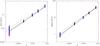 |
Fig. 11 Averaged final mass fraction ratios of vanadium to titanium and of manganese to titanium as tracers of the initial neutron excess. The meaning of the point types and colors, as well as the ranges of parameters are the same as in Fig. 9. Left: mass ratio V/Ti. The solid line is a fit given by, M(V)/M(Ti) = 14.8η0.73. The dashed line shows the relationship expected from an analytic model, Eq. (19). Right: mass ratio Mn/Ti. The solid line is a fit given by, M(Mn)/M(Ti) = 1170η0.68. The dashed line shows the relationship expected from an analytic model, Eq. (21). |
In QSE, the molar abundance of 52Fe can be written as 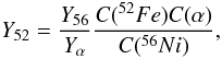 (14)From this equation and Eq. (12) one obtains
 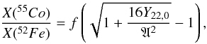 (15)where
 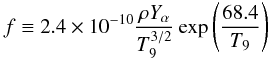 (16)is shown in Fig. 10 to only vary slightly for 3.8 > T9 ≳ 2.2 and to be nearly independent of the parameters of the Si-b nucleosynthetic calculation. Substituting approximate values for f ≃ 0.07 and A ≃ 0.011, one finally obtains the desired relationship between the abundances of 55Co and 52Fe, and the neutron excess,
 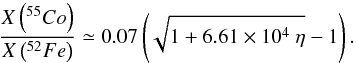 (17)This equation nicely fits the results of the nucleosynthesis calculations, as can be seen in Fig. 9. We stress that the approximations needed to derive Eq. (17) imply that it is not necessarily better than the simpler power-law fit given by Eq. (8), which is shown in the same figure. However, its derivation allows us to discern where the dependence of M(Mn)/M(Cr) on the progenitor metallicity comes from, and what its conditions of validity are. It also shows that any effect of the rest of parameters is of second order in comparison with that related to a variation in Z. Finally, it also allows us to understand that the power-law index of 0.676 is the result of the comparable magnitude of X(22Ne) and A.
4.2. Ratio of vanadium to titanium
The ratio of abundances of vanadium to titanium, V/Ti, provides an alternative way of measuring the initial neutron excess of the progenitor of a SNIa in the X-ray phase. The left hand panel of Fig. 11 shows that V/Ti traces nicely the initial neutron excess apart from η ≲ 10-4, for which there is a substantial dispersion of this ratio. The best power-law fit is 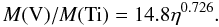 (18)Notice the similarity between the exponent of the power laws in Eqs. (8) and (18). According to Fig. 1, the ratio V/Ti obtained with the analytic model of Si-b given by Eqs. (1) and (2) matches the ratio in hydrodynamical simulations of SNIa very well.
In the X-ray epoch, vanadium and titanium come from 51Mn and 48Cr, respectively (see Table 2), whose abundances in the nucleosynthesis epoch are linked by α captures to those of 55Co and 52Fe. Using the equilibrium relationships, as in Sect. 4.1.1, the abundance ratio of 51Mn to 48Cr can be shown to be proportional to the ratio of 55Co to 52Fe, with 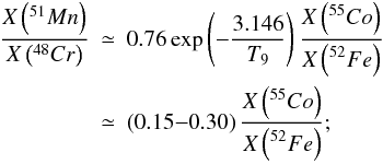 (19)i.e., the abundance ratio V/Ti is expected to range about 15−30% of the ratio Mn/Cr. Comparison of the left hand panel of Figs. 11 to 9 confirms this approximate relationship.
4.3. Ratio of manganese to titanium
The ratio of abundances of manganese to titanium, Mn/Ti, provides an alternative way of measuring the initial neutron excess in the X-ray phase. The right hand panel of Fig. 11 shows that Mn/Ti nicely traces the initial neutron excess in the whole η range explored here. The best power-law fit is 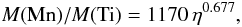 (20)which is again similar to the exponents of the power laws in Eqs. (8) and (18). According to Fig. 1, the ratio Mn/Ti obtained with the analytic model of Si-b given by Eqs. (1) and (2) shows a relative error of approximately 20% relative to the ratio in hydrodynamical simulations of SNIa. However, this error is much lower than the range of variation in M(Mn)/M(Ti) as a function of η.
In the X-ray epoch, manganese and titanium come from 55Co and 48Cr, respectively (see Table 2). Using the equilibrium relationships, the ratio of 55Co to 48Cr can be shown, as in the previous section, to be proportional to the ratio of 55Co to 52Fe, with 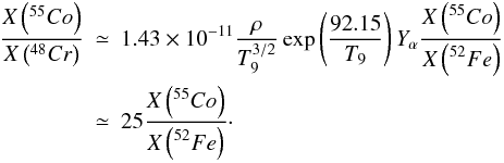 (21)Comparison of the right hand panel of Figs. 11 to 9 confirms this approximate relationship.
5. Tracers of the progenitor metallicity: optical epoch
As seen in Table 2, there are several important contributors to the abundances of the elements from scandium to iron in the optical phase, most of them unstable, which implies that their abundances vary in time. The variation in time of their ratios makes it more difficult to define in this phase a tracer of the explosion properties. However, there are interesting correlations between the progenitor metallicity and several abundance ratios in the optical phase, namely manganese to chromium, vanadium to manganese, and titanium to manganese. All these ratios share the need to measure the abundance of manganese. We have not been able to found any tracer of the progenitor metallicity in this phase that does not involve manganese.
 |
Fig. 12 Evolution with time of the abundance ratios of potential tracers of the progenitor metallicity in the optical epoch: solid black lines belong to Mn/Cr, dashed blue lines to V/Mn, and dotted red lines to Ti/Mn. For each couple of elements, the labeled curve is the one belonging to X(22Ne) = 2.5 × 10⁻⁴, whereas the other curve with the same type and color belongs to X(22Ne) = 0.075. The dot-dashed green line shows the evolution of Ti/Cr ratio, which could be used as a control variable, see Sect. 7. |
Figure 12 shows the evolution of several abundance ratios for the extreme values of the initial neutron excess explored in the present work. The separation between the curves belonging to the different η makes these abundance ratios promising tracers of the initial neutron excess.
5.1. Ratio of manganese to chromium
Among the element couples shown in Fig. 12, the ratio Mn/Cr exhibits the best behavior, because it remains nearly constant after day three. At these times, manganese is composed of 53Mn, made as 53Fe in the nucleosynthetic epoch, in a proportion higher than 80%, and the dominant isotope of chromium is 52Cr, made as 52Fe, which represents more than 90% of its abundance.
 |
Fig. 13 Averaged final mass fraction ratio Mn/Cr in the optical phase, as a function of the initial neutron excess. The meaning of the point types and colors is the same as in Fig. 9. The ranges of the parameters τrise, τ, and X(12C) are as in Fig. 9. The solid line is a fit given by, M(Mn)/M(Cr) = 2.2η0.48. |
As can be seen in Fig. 13, the ratio Mn/Cr in the optical phase is a good tracer of the initial neutron excess. The dispersion related to the different parameters used in the present calculations of Si-b is small, although it is larger for the lowest initial neutron excess. The best power-law fit is 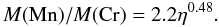 (22)
(22)
5.2. Ratio of vanadium to manganese
At the optical epoch, there are various vanadium isotopes contributing significantly to the element abundance, namely 48V, 49V, and 51V. Isotope 48V, whose parent decays in less than one day, disintegrates itself with a lifetime slightly less than the time it takes for a typical SNIa to reach maximal brightness. Isotope 49V, formed from 49Cr practically instantaneously after the explosion, has a lifetime close to one year, which makes its contribution close to constant in the whole optical epoch. Isotope 51V also forms practically instantaneously after the explosion from 51Mn, and decays with a lifetime of nearly one month. At the lowest neutron excess we considered, only 48V contributes to the vanadium abundance.
The abundance ratio of vanadium to manganese is another good tracer of the initial neutron excess, although it presents the difficulty that the ratio changes with time. The left hand panel of Fig. 14 shows this ratio and a power-law fit for two times. At 15 days, close to maximal brightness of a typical SNIa, it is given by 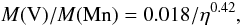 (23)whereas at 30 days, a time at which the photosphere is close to the center of the ejecta, the fit is
 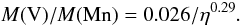 (24)
(24)
5.3. Ratio of titanium to manganese
The dominant isotope of titanium after day 10 is 48Ti, made as 48Cr, whose abundance amounts to more than 90% of the total mass of titanium. Although the lifetime of the radioactive parent of 48Ti, i.e. 48V, is 16 days, the ratio Ti/Mn changes little after day ~15 in comparison with its dependence on the initial neutron excess. The right hand panel of Fig. 14 shows that Ti/Mn can be fit by the same function of η at 15 and 30 days,  (25)
(25)
6. Tracers of the explosion conditions
As seen in the previous section, the ratios of abundances of most iron QSE-group elements are especially sensitive to the neutron excess. Consequently, it is difficult to find tracers of the rest of parameters, namely expansion timescale, temperature rise time, and initial carbon abundance. We have only found one such possible tracer, V/Mn in the X-ray epoch.
6.1. Expansion timescale: ratio of vanadium to manganese at the X-ray epoch
The most promising pairs of elements to look for a tracer of the expansion timescale, τ, are those that come from parents linked by an alpha capture in QSE, because this is the reaction type that depends the less in the n/p ratio, hence in the neutron excess. The first possibility is the pair formed by titanium and chromium, at the X-ray epoch, whose grandparents in the nucleosynthetic epoch are 48Cr and 52Fe, respectively. However, the results of the present calculations show that the ratio of their abundances is insensitive to τ.
 |
Fig. 14 Averaged final mass fraction ratios V/Mn and Ti/Mn in the optical phase, as a function of the initial neutron excess. The point types and colors in these plots refer to the time at which the ratios are drawn, blue solid circles are calculated at day 15, whereas red solid squares belong to day 30. The ranges of the parameters τrise, τ, and X(12C) are as in Fig. 9. Left: abundance ratio of vanadium to manganese. The ratios are fit by power-law functions, namely M(V)/M(Mn) = 0.018/η0.42 for the points at day 15, and M(V)/M(Mn) = 0.026/η0.29 for the points at day 30. Right: abundance ratio of titanium to manganese. In this case, the points belonging to days 15 and 30 can be reasonably fit by a single function, although it cannot be a simple power law. The fit function shown is, M(Ti)/M(Mn) = exp(−6.45−1.1lnη−0.043ln2η). |
The second possibility is the pair formed by vanadium and manganese, also at the X-ray epoch, whose grandparents are 51Mn and 55Co, respectively. Their abundance ratio is only mildly sensitive to τ and strongly dependent on η. An approximate measure of the expansion timescale would only be possible once the neutron excess is known, and only for low-metallicity progenitors, Z ≲ 0.1Z⊙. At higher values of the initial neutron excess, the ratio of vanadium to manganese abundances, V/Mn, is insensitive to τ.
Figure 15 shows the ratio V/Mn for a low-metallicity progenitor as a function of the expansion timescale. The calculated ratio depends on τ only for expansion timescales less than ~0.8 s. The dispersion introduced by the different peak-temperature distribution functions used is comparable to the difference in V/Mn for close τ, so this tracer would not even allow determining the expansion timescale with high precision. The function, ![\begin{equation} \label{eq26} M({\rm V})/M({\rm Mn})=\log\left[\log\left(1/\tau\right)^{0.7}\right]-1.7, \end{equation}](/articles/aa/full_html/2013/02/aa20309-12/aa20309-12-eq213.png) (26)provides a reasonable fit to the present results.
(26)provides a reasonable fit to the present results.
6.2. Deflagration or detonation?
Knowing the temperature rise timescale would allow discerning whether burning in the incomplete Si-b regime in SNIa proceeds through a deflagration or a detonation wave. Unfortunately, as can be expected from the discussion in Sect. 3.1.4, we did not found any pair of iron QSE-group elements whose mass ratio is sensitive to the rise time. The same applies to the determination of the initial carbon mass fraction.
7. The ratio of titanium to chromium as a control variable
We have already explained that the ratio of the abundance of titanium to that of chromium, Ti/Cr, is insensitive to the parameters of the incomplete Si-b calculation, in the limits explored in the present work; i.e., it cannot be used as a tracer of any one of these parameters, including the neutron excess. However, this does not mean that measuring Ti/Cr is useless. On the contrary, it can be utilized as a control variable to check that the SNIa properties match the predictions of the present Si-b calculations.
Figure 12 shows the evolution of Ti/Cr in time until two months after a SNIa explosion. Titanium abundance grows steadily as a result of the decay of 48V, whereas the abundance of chromium remains stable after a few hours from the thermonuclear runaway. However, the ratio Ti/Cr does not change significantly after day 30, and what is most important, it is practically the same irrespective of the metallicity of the progenitor WD. In the X-ray epoch, the full set of parameters used in the Si-b calculations leads to values of Ti/Cr in the range 0.035−0.06.
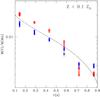 |
Fig. 15 Averaged final mass fraction ratio of vanadium to manganese as tracer of the expansion timescale, at fixed neutron excess, η = 2.27 × 10⁻⁵. The meaning of the point types and colors is the same as in Fig. 9. The results are shown for different τrise in the range 10-9−0.2 s, and X(12C) in the range 0.3−0.7. The solid line is a fit given by M(V)/M(Mn) = log [log (1/τ)0.7] −1.7. |
The profile of Ti/Cr in the ejecta of the reference SNIa model of the present work, DDTc, is flat in the region undergoing incomplete Si-b (4.3 ≤ T9,peak ≤ 5.2) with a value in the range Ti/Cr ≃ 0.025 − 0.05, whereas it rises in the inner NSE region by nearly an order of magnitude. As a result, measuring Ti/Cr might provide a way to evaluate whether the observed signal from these elements comes from a region processed to incomplete Si-b, NSE, or a mixture of both.
8. Discussion
In this work, we investigate the properties of the nucleosynthesis in the incomplete Si-b regime, using a parameterized description of the initial chemical composition and the evolution of the thermodynamic variables, in the context of SNIa. We focus the study on potential nucleosynthetic tracers of the parameters of Si-b. We discarded tracers based on the measurement of the abundance of a single element, because it would depend on the extent of combustion within the exploding WD, which is expected to vary substantially from event to event. We therefore consider abundance ratios as the most promising targets for the present study. We find that the ratios that involve elements belonging to the silicon QSE-group do not correlate well with the parameters of Si-b, so the selected ratios are those involving the lightest elements of the iron QSE-group, i.e., titanium, vanadium, chromium, and manganese. We hereby summarize the findings of this work and briefly discuss the plausibility of measuring the most interesting abundance ratios either in SNIa remnants or in SNIa near maximum brightness, the so-called photospheric epoch.
8.1. Young supernova remnants
A young supernova remnant is one in which the reverse shock, which is responsible for heating and decelerating the ejecta, has not had time to reach the center of the ejecta. This time coincides more or less with the moment when the shocked mass of the interstellar medium equals the supernova ejecta mass. Since the X-ray emission of SNIa ejecta peaks at or near the reverse shock, it can reveal the chemical composition at different locations within the remnant. Assuming chemical stratification of the ejecta, in the first thousand years or so after the explosion, where the precise time depends on a number of environment and explosion variables, the emission comes from material whose composition was set in the explosion by the incomplete Si-b process.
Measurement of the abundances of the four aforementioned elements in a young supernova remnant would provide different estimates of the initial neutron excess, related to the progenitor metallicity, which would allow a cross-check of the results. In restricted cases, it would allow roughly estimating the expansion timescale of the explosion:
-
Tracers of the initial neutron excess.
-
Tracer of the expansion timescale.
- 1.
V/Mn can be used to obtain a rough estimate of the expansion timescale only if the neutron excess has been measured previously and if the corresponding progenitor metallicity is lower than ~0.1 Z⊙. In this case, the best fit is given by Eq. (26).
- 1.
-
Control variable.
- 1.
Ti/Cr barely depends on any parameter of Si-b, so it can be used to check that the present predictions are correct or to check that the reverse shock is inside the incomplete Si-b zone. The value of Ti/Cr we found is in the range 0.035−0.06.
- 1.
Chromium and manganese have already been detected with Suzaku in a number of SNIa remnants (Yamaguchi & Koyama 2010; Yamaguchi et al. 2012). The detection of vanadium in X-rays is problematic due to its low abundance, whereas that of titanium may be made difficult by superposition of the emission from non-dominant ions of lavishly produced calcium, i.e. those emitting at a higher energy than the bulk of calcium. The emission peaks of titanium to manganese are separated well in energy, by more than ~300 eV, which ensures that their features can be resolved by the instrument XIS onboard Suzaku, as well as with future missions. For instance, the IXO proposal contemplated a resolution of 6 eV at 6 keV, with an effective area of 0.65 m2, which is ~6.5 times better than the effective area of XIS at the same energy. Thus, one can expect that detection of chromium and manganese, and perhaps titanium, in supernova remnants will be common in the future.
A quite different question is the quantitative interpretation of X-ray observations of supernova remnants, needed to obtain the desired abundance ratios. First, not all the atomic data needed to properly model X-ray emission from these elements are available at present. Second, it is difficult to estimate the physical variables that influence X-ray spectra. Hopefully, technical advances in the near future will make this interpretation more reliable.
8.2. Photospheric epoch of SNIa
The photospheric epoch of SNIa starts shortly after the explosion, and ends approximately a month later. It shares a common picture with young supernova remnant, in the sense that the optical emission is determined mainly by the position of a receding front, in this case the photosphere. While the photosphere remains far enough from the center of the ejecta, the optical emission thus comes from matter whose chemical composition was set by the incomplete Si-b process. In this epoch, it is necessary to measure the abundance of manganese to obtain any estimate of the initial neutron excess.
-
Tracers of the initial neutron excess.
-
1.
Mn/Cr again provides the best measurement of η, becauseboth their ratios vary little with time, and it correlates stronglywith the neutron excess. The best fit, which is applicable afterday five after the explosion, is given by Eq. (22).
-
2.
V/Mn varies with time owing to the different contributions of radioactive isotopes of vanadium. The best fits are given by Eq. (23) (day 15) and Eq. (24) (from day 30 on).
-
3.
Ti/Mn can be fit as a single function of η, Eq. (25), from day 10 on.
-
1.
-
Control variable. Ti/Cr varies with time but is insensitive to any of the parameters of incomplete Si-b (Fig. 12).
Hatano et al. (1999) studied the ion signatures in SNIa spectra, concluding that there are several isotopes from titanium to manganese that are potentially identifiable in the photospheric epoch, namely Ti ii, V ii, Cr i, Cr ii, Mn i, and Mn ii. However, the only elements detected so far are titanium and chromium, both in SN2002bo and SN2004eo (Stehle et al. 2005a; Mazzali et al. 2008). Continued improvement in the techniques used in the recording and interpretation of SNIa spectra, will provide better estimates of the mass of titanium, chromium, and manganese in future observations3. Obviously, the next SNIa exploding in the Milky Way will provide the opportunity to measure its chemical composition with unprecedented detail.
8.3. Final remarks
The use of the proposed abundance ratios to estimate SNIa properties is robust, in the sense that
-
1.
The profile of each one of the abundance ratios is homogeneousthroughout the region affected by incomplete Si-b. As a result, itdoes not depend on the precise position of the reverse shock(X-ray epoch) or of the photosphere (optical epoch).
-
2.
A control variable is defined, which is the ratio Ti/Cr that, if measured, would allow checking that the emitting region is within the incomplete Si-b layers.
-
3.
In SNIa models, titanium and chromium are synthesized mainly by the incomplete Si-b process. Manganese can have an additional contribution from NSE regions, whose relevance depends on both the central density of the progenitor WD at thermal runaway and the initial development of the combustion wave. Vanadium can only take contributions from a slightly wider range of peak temperatures than explored here.
It is important that the empirical correlations between abundance ratios and initial neutron excess, found as a result of the integration of the nuclear evolutionary equations, are supported by a theoretical analysis based on the properties of QSE groups in Si-b. This theoretical analysis allows us to understand the conditions under which one can expect the empirical correlations to apply. It has also been shown that the relatively low entropy of incomplete Si-b in SNIa is a necessary condition for the tight correlation between the abundance ratio Mn/Cr and the initial neutron excess. This correlation therefore cannot be extrapolated to incomplete Si-b matter in core-collapse supernovae.
It should be recalled that the relationship between the neutron excess of the progenitor WD at runaway and the metallicity of the progenitor star at zero-age main-sequence can be modified owing to electron captures during the hundreds of years of the carbon-simmering phase that precedes thermal runaway (Piro & Bildsten 2008; Badenes et al. 2008).
References
- Altavilla, G., Stehle, M., Ruiz-Lapuente, P., et al. 2007, A&A, 475, 585 [NASA ADS] [CrossRef] [EDP Sciences] [Google Scholar]
- Asplund, M., Grevesse, N., & Jacques Sauval, A. 2006, Nucl. Phys. A, 777, 1 [NASA ADS] [CrossRef] [Google Scholar]
- Badenes, C. 2010, Proc. National Academy of Science, 107, 7141 [NASA ADS] [CrossRef] [Google Scholar]
- Badenes, C., Borkowski, K. J., & Bravo, E. 2005, ApJ, 624, 198 [NASA ADS] [CrossRef] [Google Scholar]
- Badenes, C., Bravo, E., & Hughes, J. P. 2008, ApJ, 680, L33 [NASA ADS] [CrossRef] [Google Scholar]
- Blondin, S., Prieto, J. L., Patat, F., et al. 2009, ApJ, 693, 207 [NASA ADS] [CrossRef] [Google Scholar]
- Bloom, J. S., Kasen, D., Shen, K. J., et al. 2012, ApJ, 744, L17 [NASA ADS] [CrossRef] [Google Scholar]
- Bodansky, D., Clayton, D. D., & Fowler, W. A. 1968, ApJS, 16, 299 [Google Scholar]
- Bravo, E., & García-Senz, D. 2008, A&A, 478, 843 [NASA ADS] [CrossRef] [EDP Sciences] [Google Scholar]
- Bravo, E., & Martínez-Pinedo, G. 2012, Phys. Rev. C, 85, 055805 [NASA ADS] [CrossRef] [Google Scholar]
- Bravo, E., García-Senz, D., Cabezón, R. M., & Domínguez, I. 2009, ApJ, 695, 1257 [NASA ADS] [CrossRef] [Google Scholar]
- Bravo, E., Althaus, L. G., García-Berro, E., & Domínguez, I. 2011, A&A, 526, A26 [NASA ADS] [CrossRef] [EDP Sciences] [Google Scholar]
- Calder, A. C., Krueger, B. K., Jackson, A. P., et al. 2012, [arXiv:1205.0966] [Google Scholar]
- Chomiuk, L., Soderberg, A. M., Moe, M., et al. 2012, ApJ, 750, 164 [NASA ADS] [CrossRef] [Google Scholar]
- Cyburt, R. H., Amthor, A. M., Ferguson, R., et al. 2010, ApJS, 189, 240 [NASA ADS] [CrossRef] [Google Scholar]
- D’Andrea, C. B., Gupta, R. R., Sako, M., et al. 2011, ApJ, 743, 172 [NASA ADS] [CrossRef] [Google Scholar]
- Di Stefano, R., & Kilic, M. 2012, ApJ, 759, 56 [NASA ADS] [CrossRef] [Google Scholar]
- Domínguez, I., Höflich, P., & Straniero, O. 2001, ApJ, 557, 279 [NASA ADS] [CrossRef] [Google Scholar]
- Folatelli, G., Phillips, M. M., Morrell, N., et al. 2012, ApJ, 745, 74 [NASA ADS] [CrossRef] [Google Scholar]
- Foley, R. J., Simon, J. D., Burns, C. R., et al. 2012, ApJ, 752, 101 [NASA ADS] [CrossRef] [Google Scholar]
- Fuller, G. M., Fowler, W. A., & Newman, M. J. 1982, ApJS, 48, 279 [NASA ADS] [CrossRef] [Google Scholar]
- García-Senz, D., Bravo, E., & Woosley, S. E. 1999, A&A, 349, 177 [NASA ADS] [Google Scholar]
- Hatano, K., Branch, D., Fisher, A., Millard, J., & Baron, E. 1999, ApJS, 121, 233 [NASA ADS] [CrossRef] [Google Scholar]
- Hix, W. R., & Thielemann, F. 1996, ApJ, 460, 869 [Google Scholar]
- Hix, W. R., & Thielemann, F. 1999, ApJ, 511, 862 [NASA ADS] [CrossRef] [Google Scholar]
- Höflich, P., & Stein, J. 2002, ApJ, 568, 779 [NASA ADS] [CrossRef] [Google Scholar]
- Höflich, P., Gerardy, C. L., Nomoto, K., et al. 2004, ApJ, 617, 1258 [NASA ADS] [CrossRef] [Google Scholar]
- Itoh, N., Totsuji, H., Ichimaru, S., & Dewitt, H. E. 1979, ApJ, 234, 1079 [NASA ADS] [CrossRef] [Google Scholar]
- Khokhlov, A. M. 1988, 149, 91 [Google Scholar]
- Li, W., Bloom, J. S., Podsiadlowski, P., et al. 2011, Nature, 480, 348 [NASA ADS] [CrossRef] [Google Scholar]
- Lodders, K. 2003, ApJ, 591, 1220 [NASA ADS] [CrossRef] [Google Scholar]
- Maeda, K., Röpke, F. K., Fink, M., et al. 2010, ApJ, 712, 624 [NASA ADS] [CrossRef] [Google Scholar]
- Maoz, D., & Mannucci, F. 2008, MNRAS, 388, 421 [NASA ADS] [CrossRef] [Google Scholar]
- Maoz, D., Badenes, C., & Bickerton, S. J. 2012, ApJ, 751, 143 [NASA ADS] [CrossRef] [Google Scholar]
- Martínez-Pinedo, G., Langanke, K., & Dean, D. J. 2000, ApJS, 126, 493 [NASA ADS] [CrossRef] [Google Scholar]
- Mazzali, P. A., Röpke, F. K., Benetti, S., & Hillebrandt, W. 2007, Science, 315, 825 [NASA ADS] [CrossRef] [PubMed] [Google Scholar]
- Mazzali, P. A., Sauer, D. N., Pastorello, A., Benetti, S., & Hillebrandt, W. 2008, MNRAS, 386, 1897 [NASA ADS] [CrossRef] [Google Scholar]
- Meyer, B. S., Krishnan, T. D., & Clayton, D. D. 1996, ApJ, 462, 825 [NASA ADS] [CrossRef] [Google Scholar]
- Meyer, B. S., Krishnan, T. D., & Clayton, D. D. 1998, ApJ, 498, 808 [NASA ADS] [CrossRef] [Google Scholar]
- Nugent, P. E., Sullivan, M., Cenko, S. B., et al. 2011, Nature, 480, 344 [NASA ADS] [CrossRef] [Google Scholar]
- Patat, F., Chandra, P., Chevalier, R., et al. 2007, Science, 317, 924 [NASA ADS] [CrossRef] [EDP Sciences] [PubMed] [Google Scholar]
- Piro, A. L., & Bildsten, L. 2008, ApJ, 673, 1009 [NASA ADS] [CrossRef] [Google Scholar]
- Rakowski, C. E., Badenes, C., Gaensler, B. M., et al. 2006, ApJ, 646, 982 [NASA ADS] [CrossRef] [Google Scholar]
- Rauscher, T., Heger, A., Hoffman, R. D., & Woosley, S. E. 2002, ApJ, 576, 323 [NASA ADS] [CrossRef] [Google Scholar]
- Rigault, M., Copin, Y., Aldering, G., et al. 2011, in SF2A-2011: Proc. Annual meeting of the French Society of Astronomy and Astrophysics, eds. G. Alecian, K. Belkacem, R. Samadi, & D. Valls-Gabaud, 179 [Google Scholar]
- Salpeter, E. E., & van Horn, H. M. 1969, ApJ, 155, 183 [NASA ADS] [CrossRef] [Google Scholar]
- Schaefer, B. E., & Pagnotta, A. 2012, Nature, 481, 164 [NASA ADS] [CrossRef] [Google Scholar]
- Shappee, B. J., Kochanek, C. S., & Stanek, K. Z. 2012, ApJ, submitted [arXiv:1205.5028] [Google Scholar]
- Simon, J. D., Gal-Yam, A., Gnat, O., et al. 2009, ApJ, 702, 1157 [NASA ADS] [CrossRef] [Google Scholar]
- Stehle, M., Mazzali, P. A., Benetti, S., & Hillebrandt, W. 2005a, MNRAS, 360, 1231 [NASA ADS] [CrossRef] [Google Scholar]
- Stehle, M., Mazzali, P. A., & Hillebrandt, W. 2005b, Nucl. Phys. A, 758, 470 [NASA ADS] [CrossRef] [Google Scholar]
- Tanaka, M., Mazzali, P. A., Stanishev, V., et al. 2011, MNRAS, 410, 1725 [NASA ADS] [CrossRef] [Google Scholar]
- Thielemann, F.-K., Nomoto, K., & Yokoi, K. 1986, A&A, 158, 17 [NASA ADS] [Google Scholar]
- Timmes, F. X., & Woosley, S. E. 1992, ApJ, 396, 649 [NASA ADS] [CrossRef] [Google Scholar]
- Timmes, F. X., Brown, E. F., & Truran, J. W. 2003, ApJ, 590, L83 [NASA ADS] [CrossRef] [Google Scholar]
- van Kerkwijk, M. H., Chang, P., & Justham, S. 2010, ApJ, 722, L157 [NASA ADS] [CrossRef] [Google Scholar]
- Woosley, S. E., Arnett, W. D., & Clayton, D. D. 1973, ApJS, 26, 231 [NASA ADS] [CrossRef] [Google Scholar]
- Yamaguchi, H., & Koyama, K. 2010, Mem. Soc. Astron. It., 81, 382 [NASA ADS] [Google Scholar]
- Yamaguchi, H., Tanaka, M., Maeda, K., et al. 2012, ApJ, 749, 137 [NASA ADS] [CrossRef] [Google Scholar]
- Yuan, F., Quimby, R. M., Wheeler, J. C., et al. 2010, ApJ, 715, 1338 [NASA ADS] [CrossRef] [Google Scholar]
- Zingale, M., Almgren, A. S., Bell, J. B., Nonaka, A., & Woosley, S. E. 2009, ApJ, 704, 196 [NASA ADS] [CrossRef] [Google Scholar]
All Tables
All Figures
|
Fig. 1 Error in the elemental yields obtained with Eqs. (1) and (2) relative to those for the same element obtained with the thermodynamic trajectories provided by a hydrodynamic code for a SNIa model (see text for further details). Large open (red) circles give the errors belonging to a time of one day after the explosion, when the abundances of many iron-group elements are still dominated by radioactive isotopes. Small filled (blue) circles give the errors belonging to a time one hundred years after the explosion. Points belonging to some interesting couples of elements are highlighted by a small ellipse around them. For this comparison, we have only considered the layers with peak temperatures between 4.3 and 5.2 GK. |
| In the text | |
|
Fig. 2 Evolution of the chemical composition for a reference set of parameters, namely Tpeak = 4.8 109 K, τrise = 10-9 s, τ = 0.29 s, X(12C) = 0.5, X(22Ne) = 0.01. The dashed line is the temperature in 109 K. |
| In the text | |
|
Fig. 3 Distribution of maximal temperatures in the incomplete Si-burning region obtained from a suite of SNIa models. Left: one-dimensional delayed detonation models DDTc (red crosses, Badenes et al. 2005) and DDTf (red solid squares), a sub-Chandrasekhar model (blue stars) from Bravo et al. (2011, fourth row in their Table 2), and three-dimensional delayed detonation model TURB7 from Bravo et al. (2009, red empty squares,). The solid line is a fit to the data given by, |
| In the text | |
|
Fig. 4 Final mass fraction ratio Mn/Cr, at a time of 100 yrs after the explosion, as a function of peak temperature in incomplete Si-b for different maximal densities (point type) and initial neutron excesses (color online). The maximal densities are given by either Eq. (6) (filled circles), or by a factor of two higher (triangles), or lower (crosses) than Eq. (6). The initial neutron excesses are η = 2.27 × 10⁻⁴ (red), 9.09 × 10⁻⁴ (blue), and 6.82 10-3 (black), increasing from bottom to top. |
| In the text | |
|
Fig. 5 Comparison of relevant timescales as a function of the initial density. Solid line: expansion timescale, computed as the free-fall or hydrodynamic timescale, |
| In the text | |
|
Fig. 6 Evolution of the chemical composition for a rise time to the maximal temperature different from that in the reference set of parameters (Fig. 2). Left: slower rise to the peak temperature, τrise = 10-5 s. Right: rise time comparable to the expansion timescale, τrise = 0.1 s. |
| In the text | |
|
Fig. 7 Evolution of the chemical composition for different expansion timescales and initial carbon abundances than in the reference set of parameters (Fig. 2). Left: slower expansion timescale, τ = 0.72 s. Right: smaller carbon abundance, X(12C) = 0.3. |
| In the text | |
|
Fig. 8 Evolution of the chemical composition for an initial neutron excess higher than in the reference set of parameters (Fig. 2), X(22Ne) = 0.075. |
| In the text | |
|
Fig. 9 Averaged final mass fraction ratio Mn/Cr as a function of the initial neutron excess. The average mass fractions are drawn either from the fit to the distribution of maximum temperatures given in the left panel of Fig. 3 (red circles) or from a uniform distribution function representative of the models shown in the right panel of the same figure (blue crosses). In both cases, the results are shown for different τrise in the range 10-9−0.2 s, τ in the range 0.10−0.90 s, and X(12C) in the range 0.3−0.7. The solid line is a fit given by, M(Mn)/M(Cr) = 49.1η0.676. The dashed line shows the relationship expected from an analytic model, Eq. (17). Green stars give the mass fraction ratio Mn/Cr for high-entropy conditions (see text for details). |
| In the text | |
|
Fig. 10 Nuclear evolution as a function of temperature during expansion and cooling. Left: evolution of the mass fractions of 55Co (solid lines), 52Fe (dashed lines), and α (dot-dashed lines), for six different sets of parameters, as given in Table 3. The dotted lines show the quantity f, defined in Eq. (16). Right: evolution of the molar fluxes of the main reactions contributing to the abundance of 55Co for the same set of parameters as in Fig. 2. Reactions building 55Co are drawn as solid lines, reactions destroying it are drawn as dashed lines, and the absolute value of the net rate of dY(55Co)/dt is drawn as a dotted line. Upper curves are for the reactions 54Fe + p ⇆ 55Co + γ, in which both line types are nearly indistinguishable. The middle curves are for the reactions 56Ni + γ ⇆ 55Co + p. Finally, the bottom curves are for the reactions 55Fe + p ⇆ 55Co + n. |
| In the text | |
|
Fig. 11 Averaged final mass fraction ratios of vanadium to titanium and of manganese to titanium as tracers of the initial neutron excess. The meaning of the point types and colors, as well as the ranges of parameters are the same as in Fig. 9. Left: mass ratio V/Ti. The solid line is a fit given by, M(V)/M(Ti) = 14.8η0.73. The dashed line shows the relationship expected from an analytic model, Eq. (19). Right: mass ratio Mn/Ti. The solid line is a fit given by, M(Mn)/M(Ti) = 1170η0.68. The dashed line shows the relationship expected from an analytic model, Eq. (21). |
| In the text | |
|
Fig. 12 Evolution with time of the abundance ratios of potential tracers of the progenitor metallicity in the optical epoch: solid black lines belong to Mn/Cr, dashed blue lines to V/Mn, and dotted red lines to Ti/Mn. For each couple of elements, the labeled curve is the one belonging to X(22Ne) = 2.5 × 10⁻⁴, whereas the other curve with the same type and color belongs to X(22Ne) = 0.075. The dot-dashed green line shows the evolution of Ti/Cr ratio, which could be used as a control variable, see Sect. 7. |
| In the text | |
|
Fig. 13 Averaged final mass fraction ratio Mn/Cr in the optical phase, as a function of the initial neutron excess. The meaning of the point types and colors is the same as in Fig. 9. The ranges of the parameters τrise, τ, and X(12C) are as in Fig. 9. The solid line is a fit given by, M(Mn)/M(Cr) = 2.2η0.48. |
| In the text | |
|
Fig. 14 Averaged final mass fraction ratios V/Mn and Ti/Mn in the optical phase, as a function of the initial neutron excess. The point types and colors in these plots refer to the time at which the ratios are drawn, blue solid circles are calculated at day 15, whereas red solid squares belong to day 30. The ranges of the parameters τrise, τ, and X(12C) are as in Fig. 9. Left: abundance ratio of vanadium to manganese. The ratios are fit by power-law functions, namely M(V)/M(Mn) = 0.018/η0.42 for the points at day 15, and M(V)/M(Mn) = 0.026/η0.29 for the points at day 30. Right: abundance ratio of titanium to manganese. In this case, the points belonging to days 15 and 30 can be reasonably fit by a single function, although it cannot be a simple power law. The fit function shown is, M(Ti)/M(Mn) = exp(−6.45−1.1lnη−0.043ln2η). |
| In the text | |
|
Fig. 15 Averaged final mass fraction ratio of vanadium to manganese as tracer of the expansion timescale, at fixed neutron excess, η = 2.27 × 10⁻⁵. The meaning of the point types and colors is the same as in Fig. 9. The results are shown for different τrise in the range 10-9−0.2 s, and X(12C) in the range 0.3−0.7. The solid line is a fit given by M(V)/M(Mn) = log [log (1/τ)0.7] −1.7. |
| In the text | |
Current usage metrics show cumulative count of Article Views (full-text article views including HTML views, PDF and ePub downloads, according to the available data) and Abstracts Views on Vision4Press platform.
Data correspond to usage on the plateform after 2015. The current usage metrics is available 48-96 hours after online publication and is updated daily on week days.
Initial download of the metrics may take a while.