| Issue |
A&A
Volume 550, February 2013
|
|
|---|---|---|
| Article Number | A57 | |
| Number of page(s) | 14 | |
| Section | Interstellar and circumstellar matter | |
| DOI | https://doi.org/10.1051/0004-6361/201219837 | |
| Published online | 24 January 2013 | |
Herschel/HIFI observations of [C II] and [13C II] in photon-dominated regions⋆
1
I. Physikalisches Institut, Universität zu Köln,
Zülpicher Str. 77,
50937
Köln,
Germany
e-mail: This email address is being protected from spambots. You need JavaScript enabled to view it.
2
Department of Physics and Astronomy, Johns Hopkins
University, 3400 North Charles
Street, Baltimore,
MD
21218,
USA
3
Observatorio Astronómico Nacional, Apdo. 112, 28803 Alcalá de Henares,
Madrid,
Spain
4
Centro de Astrobiología (INTA-CSIC), Ctra. M-108, km.
4, 28850
Torrejón de Ardoz,
Spain
5
California Institute of Technology, Cahill Center for Astronomy and Astrophysics
301-17, Pasadena,
CA
91125,
USA
6
SRON Netherlands Institute for Space Research,
Landleven 12, 9747 AD
Groningen, The
Netherlands
7
Kapteyn Astronomical Institute, University of
Groningen, PO box
800, 9700 AV
Groningen, The
Netherlands
8
University of Michigan, Ann Arbor, MI
48197,
USA
Received: 18 June 2012
Accepted: 14 November 2012
Abstract
Context. Chemical fractionation reactions in the interstellar medium can result in molecular isotopologue abundance ratios that differ by many orders of magnitude from the isotopic abundance ratios. Understanding variations in the molecular abundance ratios through astronomical observations provides a new toolto sensitively probe the underlying physical conditions.
Aims. Recently, we have introduced detailed isotopic chemistry into the KOSMA-τ model for photon-dominated regions (PDRs), which allows calculating abundances of carbon isotopologues as a function of PDR parameters. Radiative transfer computations then allow to predict the observed [C ii]/[13C ii] line intensity ratio for specific geometries. Here, we compare these model predictions with new Herschel observations.
Methods. We performed Herschel/HIFI observations of the [C ii] 158 μm line in a number of PDRs. In all sources, we observed at least two hyperfine components of the [13C ii] transition, allowing determination of the [C ii]/[13C ii] intensity ratio, using revised intrinsic hyperfine ratios. Comparing the observed line ratios with the predictions from the updated KOSMA-τ model, we identify conditions under which the chemical fractionation effects are important, and not masked by the high optical depth of the main isotopic line.
Results. An observable enhancement of the [C ii]/[13C ii] intensity ratio due to chemical fractionation depends mostly on the source geometry and velocity structure,and to a lesser extent on the gas density and radiation field strength. The enhancement is expected to be largest for PDR layers that are somewhat shielded from UV radiation, but not completely hidden behind a surface layer of optically thick [C ii]. In our observations the [C ii]/[13C ii] integrated line intensity ratio is always dominated by the optical depth of the main isotopic line. However, an enhanced intensity ratio isfound for particular velocity components in several sources: in the red-shifted material in the ultracompact H ii region Mon R2, in the wings of the turbulent line profile in the Orion Bar, and possibly in the blue wing in NGC 7023. Mapping of the [13C ii] lines in the Orion Bar gives a C+ column density map, which confirms the temperature stratification of the C+ layer, in agreement with the PDR models of this region.
Conclusions. Carbon fractionation can be significant even in relatively warm PDRs, but a resulting enhanced [C ii]/[13C ii] intensity ratio is only observable for special configurations. In most cases, a reduced [C ii]/[13C ii] intensity ratiocan be used instead to derive the [C ii] optical depth, leading to reliable column density estimates that can be compared with PDR model predictions. The C+ column densities show that, for all sources, at the position of the [C ii] peak emission, the dominant fraction of the gas-phase carbon is in the form of C+.
Key words: ISM: abundances / ISM: clouds / ISM: structure
Herschel is an ESA space observatory with science instruments provided by European-led Principal Investigator consortia and with important participation from NASA.
© ESO, 2013
1. Introduction
Isotopic abundance ratios of metals such as C, N and O in the interstellar medium (ISM) reflect the star formation history of the gas. Observations of molecular isotopic line ratios at (sub)mm wavelengths are a common way to study the cumulative effect of star formation in the Milky Way (e.g. Wilson 1999).
Isotopic fractionation of carbon in the ISM, i.e. the 12C/13C ratio in various species, is driven mainly by the fractionation reaction  that provides a significant energy excess for binding the 13C atoms to the oxygen (Langer et al. 1984). Thus chemical fractionation of carbon is important even for relatively warm gas, as long as there is a significant fraction of ionized carbon available1. The reaction (C 1) favors formation of 13CO and depletion of 13C+ at low temperatures, shifting the fractional abundances of the two species relative to the normal solar isotopic ratio. However, it competes with isotope-selective dissociation governed by different shielding due to dust, H2 and other CO isotopologues (Visser et al. 2009).
A systematic discussion of the observational results on carbon fractionation was presented by Keene et al. (1998) for dense molecular clouds and Liszt (2007) for diffuse clouds. From observations of [13C i] and 13C18O in the Orion Bar Keene et al. (1998) found little evidence for chemical fractionation, but instead noticed a contradiction between the chemical models, predicting a slight relative enhancement of 13C and a corresponding reduction of 13C18O, and the observations which showed the opposite effect. In contrast to the CO results, Sakai et al. (2010) found clear evidence for fractionation in C2H in the dark cloud TMC 1. In agreement with previous results (Sonnentrucker et al. 2007; Sheffer et al. 2007; Burgh et al. 2007), Liszt (2007) summarized the clear observational evidence for the CO fractionation in translucent and diffuse clouds. They confirmed that the fractionation reaction (C 1) dominates the carbon chemistry for densities nH2 ≥ 100 cm-3 and provided new low-temperature reaction rates, but also showed the importance of the CO destruction in reactions with He+ at lower densities.
In Paper I (Röllig & Ossenkopf 2013), we have presented results from the updated KOSMA-τ PDR model, which includes full isotopic chemistry and provides isotopologue ratios for key species. Comparing the 12C+/13C+ fractionation ratios with the elemental isotopic ratio, we have noted that
-
the fractionation ratio is always higher than, or equal to, the elemental ratio, i.e. 13C+ is always underabundant with respect to C+,
-
the fractionation ratio equals to the elemental ratio at low AV values, but increases significantly at higher AV.
However, two competing processes affect the [C ii]/[13C ii] ratio in PDRs: chemical fractionation raises the [C ii]/[13C ii] intensity ratio relative to the elemental abundance ratio, while the optical depth of the main isotopic line lowers its intensity relative to the [13C ii] transitions.
[13C ii] was first spectrally resolved through early heterodyne observations using the Kuiper Airborne Observatory (KAO, e.g. Boreiko et al. 1988; Boreiko & Betz 1996). This work found no increase in the corresponding [C ii]/[13C ii] intensity ratio, but did infer a reduction relative to the isotopic elemental ratio indicating a significant optical depth of the main isotopic line. With the low spatial and velocity resolution of these observations, it was, however, impossible to determine whether this average reduction occurs for all density or velocity components within the beam, or whether individual components, dominated by either of the two competing processes may be present. Given these issues it is clear that high velocity resolution, preferentially covering a wide range of conditions, is required to ascertain the impact of the two processes in PDRs.
The HIFI instrument (de Graauw et al. 2010) on-board the Herschel Space Observatory (Pilbratt et al. 2010) enabled for the first time systematic observations of [13C ii], with sensitivity and high spatial resolution, throughout the ISM. This allows studies of the 12C/13C ratio in different environments, by comparing the observations with theoretical predictions. We detected [13C ii] in four bright PDRs and use these observations to look for signatures of the carbon chemical fractionation in the warm PDR gas, or determine the optical depth and column density of C+.
In Sect. 2 we elaborate on the detailed theoretical predictions for the 12C+/13C+ and the resulting [C ii]/[13C ii] intensity ratio under varying physical conditions, based on the KOSMA-τ PDR model computations. In Sect. 3 we present the HIFI observations of [C ii] and [13C ii]. Section 4 discusses the observational results for the Orion Bar, Mon R2, NGC 3603, Carina, and NGC 7023 and Sect. 5 concludes with a summary of the agreements and discrepancies between the models and observations.
2. Model predictions for the [CII]/[13CII] ratio
The development of theoretical models for PDRs is an active field of research, because of the complex interplay of geometrical constraints, properties of the UV field, and chemical and physical processes in the gas (Röllig et al. 2007). Because of this complexity, all models with a detailed description of the PDR chemistry are currently restricted to one-dimensional geometries, therefore describing PDRs either as plane-parallel slabs or as (an ensemble of) spheres. However, real astronomical sources, like the prototypical Orion Bar PDR, show more complex geometries, containing elements of both descriptions, e.g. a large-scale plane-parallel configuration with a clumpy small-scale structure, better described by an ensemble of spherical cores (see e.g. Hogerheijde et al. 1995).
We consider both limiting cases in the framework of the KOSMA-τ PDR model, a code designed to simulate spherical clumps, which however can approximate a plane-parallel PDR by considering very massive clumps (M ≥ 100 M⊙) that form an almost plane-parallel structure in their outer layers. This approach allows us to use the new implementation of the fractionation network in the KOSMA-τ PDR model code and to easily compare the results with predictions of other PDR models (see Röllig et al. 2007) that currently do not include isotopic chemical networks.
2.1. Model setup
The KOSMA-τ PDR model assumes a spherical cloud geometry exposed to isotropic UV illumination, measured in units of the interstellar radiation field, χ0 (Draine 1978). Input parameters are: the hydrogen density at the surface, nsurf, the UV field, χ, and the cloud mass, M. The density structure assumes a power-law increase, nH(r) = nsurf(r/R0)-1.5, from the surface to 1/5 of the outer radius, R0, and a constant density further in. For the computations presented here, we keep the metallicity at a solar value and assume a standard elemental isotopic ratio of 12C/13C of 67 (Wakelam & Herbst 2008). The actual elemental isotopic ratio is subject to systematic variations with galactocentric radius (Wilson 1999). All the sources discussed in Sect. 3.2 are relatively nearby, however, even within the solar neighborhood noticeable variations exist, with values between 57 and 78. The value of 67 we adopt matches the ratio observed in Orion (Langer & Penzias 1990, 1993). We assume an uncertainty of 15% for the elemental abundance ratio.
The PDR model iteratively computes the steady-state chemistry, the local cooling and heating rates, and the radiative transfer to predict the volume density of various species as a function of radius and the resulting intensity of the emitted line and continuum radiation. The assumption of an isotropic UV illumination is not a fundamental limitation when comparing different geometries. The penetration of an isotropic radiation field can be computed from that of a uni-directional radiation field by rescaling the optical depth according to the formalism in Flannery et al. (1980) and vice versa. Röllig et al. (2007) showed a very good match of the different PDR models when such rescaling was applied. When re-interpreting the KOSMA-τ results for a uni-directional illumination, one thus has to scale the width of the outer layers relative to the given scale.
2.2. The effect of chemical fractionation on the [CII]/[13CII] ratio
Paper I has already provided some predictions for clump-integrated intensities for 13C-bearing species in the case of a spherical PDR. To understand in detail how the chemical fractionation structure translates into an observable [C ii]/[13C ii] intensity ratio, we first investigate how the depth-dependent carbon fractionation affects the local [13C ii] and [C ii] emissivity. We use a simplified, plane-parallel configuration described by two parameters only: the density and the impinging UV field. In the resulting one-dimensional PDR, different layers reflect the decreasing UV penetration. This allows disentangling their relative contribution to the observed [C ii]/[13C ii] intensity ratio. This approach ignores all effects resulting from uncertainties regarding cloud geometry, as well as the effect of line optical depth along the line of sight to the observer.
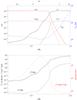 |
Fig. 1 Top: abundance distribution of C+ and CO and the corresponding 13C isotopologues for a model with nsurf = 104 cm-3, 1000 χ0 and 1000 M⊙. The blue curve shows the corresponding gas temperature structure determining the emissivity. Bottom: resulting integrated optically thin line emissivity ∫ϵdv in K km s-1/(cm-3 pc) for the [C ii] and [13C ii] lines (black curves) as a function of the clump radius. The red line shows the intensity ratio provided by the two curves. |
Figure 1 shows the temperature and abundance structure of the main carbon-bearing species and the resulting [C ii] and [13C ii] line emissivities as a function of the depth from the surface into the cloud for an example model with a density at cloud surface of 104 cm-3 and a radiation field of 1000χ0. The local [C ii] line emissivity can be computed assuming a two-level system 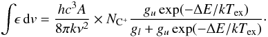 (1)With ΔE = hν = k × 91.2 K, the statistical weights gu = 4 and gl = 2, and the Einstein-A coefficient of A = 2.3 × 10⁻⁶ s-1 (Wiese & Fuhr 2007), this gives
 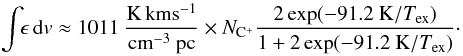 (2)The excitation temperature, Tex, is obtained from the detailed balance of collisional excitation by H2 molecules (Flower & Launay 1977), atomic hydrogen (Launay & Roueff 1977), and electrons (Wilson & Bell 2002), and radiative de-excitation and trapping2. For [13C ii], we sum over all hyperfine components. The emissivity represents the integrated line intensity per hydrogen column density, without any correction for the line optical depth.
In this example model, most of the [C ii] emission stems from the cloud surface. Here all carbon is in ionized form and, at high temperatures, the C+/13C+ fractionation ratio is equal to the elemental isotopic abundance ratio, resulting in a [C ii]/[13C ii] intensity ratio that matches the elemental ratio. Deep inside the cloud, where most of carbon is in the form of CO and 13C+ is only produced by cosmic ray ionized He+, the intensity ratio is enhanced by about a factor of ten relative to the elemental isotopic ratio. However, the C+ abundance is reduced by six orders of magnitude, so that the enhanced ratio is obscured by by the strong surface emission. The region where chemical fractionation may be detectable is thus the transition zone from C+ to CO where the C+/13C+ fractionation ratio amounts to a few hundred and the intensity is only a factor of ten weaker than the surface value (around r/R0 = 0.73 in Fig. 1). The actual emissivity ratio can be boosted to values above the fractionation ratio by radiative excitation of C+ in the cool inner regions. As C+ “feels” the strong line emission from the surface, the [C ii] excitation temperature can increase above the kinetic temperature, while the [13C ii] excitation temperature closely follows the kinetic temperature. Due to the exponential term in Eq. (2) this can provide up to a factor of ten enhancement of the [C ii]/[13C ii] intensity ratio in cold gas at moderate densities, deeper into the cloud.
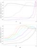 |
Fig. 2 Differences between [C ii] emissivity and [13C ii] emissivity multiplied by the standard elemental isotopic ratio of 67 showing conditions where a increased C+/13C+ fractionation ratio turns into an observable increased [C ii]/[13C ii] intensity ratio. The upper plot uses a radiation field of 1000χ0 and varies the surface gas density: 103 cm-3 (black), 104 cm-3 (grey), 105 cm-3 (blue), 106 cm-3 (red). The lower plot uses a gas density of nsurf = 104 cm-3 and varies the radiation field: 1χ0 (black), 10χ0 (grey), 100χ0 (blue), 103χ0 (cyan), 104χ0 (green), 105χ0 (red), 106χ0 (orange). The dashed line at 10 K km s-1 (cm-3 pc)-1 gives a rough indication what differences might be observable with current technology in a deep integration. |
To better evaluate, under which conditions we might observationally detect chemical fractionation, we compute the difference between the [C ii] emissivity and the [13C ii] emissivity scaled by the elemental abundance ratio. This quantity does not directly reflect the intensity ratio, as shown in Fig. 1 but its enhancement indicates conditions, under which an increased C+/13C+ fractionation ratio eventually turns into an observable increased [C ii]/[13C ii] intensity ratio. Figure 2 shows the emissivity difference as a function of the distance from the cloud surface for varying PDR parameters. In the upper panel, we vary the gas density for a constant radiation field of 1000χ0 while the lower panel shows the impact of a varying radiation field for a constant gas density of nsurf = 104 cm-3. Whenever the difference is lower than about 1 K km s-1 (cm-3pc)-1 no [C ii] enhancement is practically observable, either because the [13C ii] emission is too weak, or because no enhanced C+/13C+ fractionation ratio is present. Three factors determine the detectability of an enhanced fractionation ratio in the optically thin approximation: (i) the radiation field has to be strong enough to produce a significant column of ionized carbon; (ii) the corresponding layer has to be cool enough, so that the reaction (C 1) is effective; and (iii) the layer of enhanced C+/13C+ needs to be thick enough to couple efficently to the telescope beam. Paper I has shown that these factors can be met for a wide range of conditions, provided that there is a sufficient mass of dense gas. With at least 1 M⊙ at densities of 104 cm-3, a significant fractionation layer is formed even at high UV fields. In the upper panel of Fig. 2 we see, however, that at densities of 105 cm-3 or above, the C+–CO transition layer, producing an enhanced [C ii]/[13C ii] intensity ratio associated with strong emission, is very thin. The lower panel shows that we find only low [C ii] intensities from clumps exposed to radiation fields of 10χ0 or below, making [C ii] observations difficult. However, for all higher radiation fields, fractionation should be detectable. When considering the full range of parameters, we find some degeneracy, in the sense that for higher densities fractionation may also be observable at low UV fields. The ideal environment for an increased C+/13C+ fractionation ratio is thus mildly shielded gas in classical PDRs with χ ≳ 100χ0 and densities in the range 104−105 cm-3.
2.3. Radiative transfer effects and the [CII]/[13CII] ratio
The [C ii] optical depth can be computed in the same way as the emissivity (Eq. (2)) through 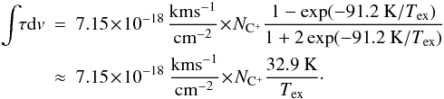 (3)For a Gaussian velocity distribution this is equal to
  (4)where
  denotes the peak optical depth and Δv the FWHM line width.
Inversely, we can determine the optical depth from the measured [C ii]/[13C ii] intensity ratio (IR), across the line from the known the C+/13C+ fractionation ratio (FR), assuming optically thin [13C ii] emission and the same excitation temperatures of [C ii] and [13C ii]: ![Mathematical equation: \begin{equation} {{\it IR}_\nu \over {\it FR}}= {1 - \exp(-\tau_{\rm [C{\mathsc II}]}) \over \tau_{\rm [C {\mathsc II}]}}\cdot \label{eq_optdepth} \end{equation}](/articles/aa/full_html/2013/02/aa19837-12/aa19837-12-eq56.png) (5)For the line integrated intensity ratio, one has to take into account the broadening of the [C ii] line due to its opacity. For a Gaussian velocity distribution and a line-center optical depth
(5)For the line integrated intensity ratio, one has to take into account the broadening of the [C ii] line due to its opacity. For a Gaussian velocity distribution and a line-center optical depth  , the increase in the line width can be approximated as
  . The average optical depth determined from the integrated line intensity is then3
 (6)To quantify the impact of the line-of-sight optical depth on the [C ii]/[13C ii] intensity ratio we have to switch from the semi-infinite plane-parallel description to a finite geometry. This requires a description for the C+ column density not only in the direction toward the illuminating source, but also on the line of sight toward the observer. This is naturally taken into account when using the clumpy picture that forms the base of the KOSMA-τ model, i.e. considering the case of a spherical PDR. It introduces the clump mass, i.e. the absolute radius of the clump, as a third independent parameter4. By integrating over the full volume of each clump and averaging the intensity over the projected area, we mimic the case of a fractal cloud, consisting of an ensemble of many clumps, where individual structures cannot be resolved (Stutzki et al. 1998).
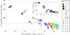 |
Fig. 3 Clump integrated intensity ratio ∫I([C ii])dv/∫I([13C ii])dv vs. [C ii] intensity from the KOSMA-τ model for different parameters. The model parameters n, M, and χ, are coded as size, shape, and color of the respective symbols. The red horizontal line denotes the assumed elemental abundance ratio [12C]/[13C] of 67. The insert demonstrates the underlying column density ratio for the different clumps. For [13C ii], we sum over all hyperfine components. |
In Fig. 3 we compare the ratio of clump-averaged integrated line intensities, ∫I([C ii])dv/∫I([13C ii])dv for a wide range of densities, clump masses and impinging radiation fields. The insert shows the underlying mean column density ratio for the clumps producing the observed intensity ratio (see Paper I).
While the column density ratio falls above the elemental isotopic ratio for all model clumps, this does not hold for the [C ii]/[13C ii] intensity ratio. Models with low densities and all models with χ > 100 show an intensity ratio below the elemental ratio, down to a value of 38. In these models, the column density ratio is close to the elemental ratio, so that the reduced intensity ratio is a direct measure of the optical depth of the main isotopic line through Eq. (5). The decrease in the integrated line intensity ratio by a factor two corresponds to a moderate [C ii] optical depth, ⟨ τ ⟩ ≈ 1.6 or  , respectively, for the individual clumps. That means that in all models exposed to high UV fields, an ionized carbon layer of about the same column density is formed, independent of the other clump parameters. This is naturally explained by the transition from C+ to CO at about AV ≈ 0.2. Different PDR parameters only change the physical depth and temperature of this transition point. Higher [C ii] optical depths only occur if multiple clumps overlap on the line of sight, spatially and in velocity, without mutually shielding the impinging UV field, i.e. in special geometries.
In the clump-integrated picture, only models with low UV field χ and high densities trace the chemical fractionation, showing an intensity ratio that is enhanced relative to the elemental abundance ratio. A detailed comparison shows that even for those clumps some line saturation occurs, so that the intensity ratio does not measure the true C+/13C+ fractionation ratio, but falls below it. This result is in contrast to the pure emissivity considerations in Sect. 2.2, which indicated that medium-density clumps produce an enhanced intensity ratio.
Optical depth effects are always significant in the considered geometry, with similar column densities of C+ toward the illuminating sources and toward the observer. C+ is abundant down to a shielding gas and dust column of AV ≈ 1 (see Fig. 1). If all carbon is ionized in this column, it provides NC + ≈ 2.5 × 1017 cm-2, corresponding to a [C ii] optical depth of 0.8 for a slightly subthermal excitation temperature of Tex = 50 K and the line width of 1.5 km s-1 used in the model. This implies that in isotropic configurations with narrow lines, as in the clumpy PDR model, [C ii] always turns slightly optically thick when the condition for an efficient fractionation is met. Hence, we find a relatively constant [C ii] optical depth of 0.8–1.6 for all clumps that are large enough to contain the critical column for AV = 1 and are exposed to a radiation field strong enough to ionize the carbon atoms. As a consequence, we expect a behavior as shown in Fig. 3 for isotropic PDRs with narrow line widths. That is the fractionation in the C+/13C+ abundance ratio seen in the local [C ii]/[13C ii] emissivity ratio in Sect. 2.2, is hidden from the observer by an optical depth close to unity in this case.
Detection of the true fractionation ratio, i.e. in the C+/13C+ column densities, through the observed [C ii]/[13C ii] intensity ratio requires optically thin [C ii] emission, either through a much larger velocity dispersion (see Eq. (4)), or an anisotropic geometry that provides a higher column of gas toward the source of UV photons than along the line-of-sight toward the observer. Only in such a configuration we can expect to detect chemical fractionation through the [C ii]/[13C ii] intensity ratio matching the predictions from Sect. 2.2. In contrast, we may also find edge-on configurations with a higher column density along the line of sight toward the observer than toward the illuminating sources (see the Orion Bar in Sect. 4.1) where the [C ii] optical depth may grow beyond 2, resulting in an intensity ratio much below the local C+/13C+ fractionation ratio.
Altogether, we conclude that in most PDRs with bright [C ii] emission, it will be difficult to infer significant fractionation in the C+ column densities, i.e. the fractionation ratio will match the elemental abundance ratio, while the intensity ratio is dominated by the optical depth of the [C ii] line, pushing it below the elemental ratio. In those cases, we can only use the intensity ratio to compute the C+ column density through Eqs. (5) and (3). This is an essential parameter to compare with models for deriving e.g. the ionization degree or the photoelectric heating efficiency. Some carbon fractionation may be detectable through an increased [C ii]/[13C ii] intensity ratio compared to the elemental abundance ratio in sources with high densities and moderate UV fields, in case of a favorable geometry or relatively broad line width. However, even in these cases it may be impossible to deduce the exact C+/13C+ fractionation ratio due to the optical depth effects.
3. Observations
3.1. [13CII] spectroscopy
C+ has a single fine structure transition, [C ii]  , at 1900.537 GHz, which for 13C+ is split into three hyperfine components due to the unbalanced spin of the additional neutron. The frequencies of these transitions have been determined by Cooksy et al. (1986) based on a combination of laser magnetic resonance measurements and ab-initio computations of Schaefer & Klemm (1970). Our observations from Sect. 4.1.2 confirm these frequencies with an accuracy of about 3 MHz, as valocities of the relatively narrow [C ii] and [13C ii] lines in the Orion Bar match each other, as well as numerous molecular transitions, to within 0.5 km s-1.
We have computed the relative line strengths expected for the three hyperfine transitions in local thermodynamic equilibrium (LTE), which – for a magnetic dipole transition – are given by  (7)(Eq. (8) in Garstang 1995, normalized to unity). Here, J′ = 3/2 and J = 1/2 are the total electronic angular momenta for the upper and lower states, I = 1/2 is the nuclear spin of the 13C nucleus, F′ and F are the total angular momenta (including nuclear spin) for the upper and lower states, and the curly brackets denote the Wigner 6j-symbol. This expression – based on the standard assumptions that magnetic dipole (M1) radiation dominates over electric quadrupole (E2) radiation, and that the Hamiltonian commutes with all relevant angular momentum operators – yields a ratio of 0.625:0.25:0.125 for the F′ − F = 2−1:1−0:1−1 transitions5. All spectroscopic parameters are summarized in Table 1.
Spectroscopic parameters of the [13C ii] transition.
3.2. HIFI measurements
We performed [13C ii] observations using the HIFI instrument (de Graauw et al. 2010) on-board Herschel (Pilbratt et al. 2010) toward four bright PDRs, in the framework of the guaranteed time key programs HEXOS (Bergin & Herschel Hexos Team 2011) and WADI (Ossenkopf et al. 2011). The first region is the Orion Bar (map center: 5h35m20.81s, −5°25′17.1′′), an edge-on, almost linear PDR at a distance of 415 pc (Menten et al. 2007), formed by material of the Orion Molecular Cloud 1 (OMC-1) exposed to the radiation from the Trapezium cluster with a FUV flux of 4−5 × 10⁴χ0 in terms of the Draine (1978) field. Previous, spectrally unresolved observations of [C ii] in the Orion Bar have been carried out by Stacey et al. (1993) and Herrmann et al. (1997) using the Kuiper Airborne Observatory (KAO). With an edge-on configuration, the Orion Bar PDR is an improbable candidate for the detection of 13C+ fractionation because of the high column density of C+ along the line of sight. However, fractionation effects may be observable if the [C ii] emission is dominated by the clumpy structure as seen by Hogerheijde et al. (1995) and Lis & Schilke (2003), who found clumps with a density well above 106 cm-3 embedded in a more widely distributed “interclump” medium with a density of 104−2 × 105 cm-3 (Simon et al. 1997). Moreover, the gas in front and behind the main Orion Bar should have a more favorable geometry. By mapping [13C ii], we are able to distinguish between these three regions.
The second PDR is formed by the molecular interface around the ultracompact H ii region Mon R2 at a distance of 830 pc (6h07m46.2s, −6°23′08.0′′). Due to its larger distance, the PDR is weaker in [C ii] than the Orion Bar, in spite of the higher FUV intensity from the central source of about 3 × 10⁵χ0 (Fuente et al. 2010). The almost spherical PDR geometry around the H ii region provides a situation close to the plane-parallel model from Sect. 2.2, with two PDR layers at high velocities behind and in front of the H ii region along the line of sight toward the center. The velocity dispersion of up to 10 km s-1 (e.g. Ginard et al. 2012) assures a low optical depth at high integrated line intensities, making Mon R2 one of the best candidates to detect an enhanced [C ii]/[13C ii] intensity ratio (Pilleri et al. 2012a). The situation is, however, complicated by the unknown effect of the outflows that have been observed on a somewhat larger scale (Xu et al. 2006).
The third PDR is the clump MM2 close to NGC 3603, at a distance of about 6 kpc (Stolte et al. 2006) (11h15m10.89s, −61°16′15.2′′), illuminated by a FUV flux of about 104χ0 from the OB stars in NGC 3603 (Röllig et al. 2011). The fourth source is the Carina Nebula at a distance of about 2.3 kpc (Smith 2006), illuminated by the OB stars in the massive clusters Trumpler 14 and 1,6 with a FUV flux of about 4 × 10³χ0 (Okada et al. 2013). Here, we observed two interfaces: the Carina North PDR (10h43m35.14s, −59°34′04.3′′) close to Trumpler 14, and the Carina South PDR (10h45m11.54s, −59°47′34.3′′) south of η Car, including the core IRAS-10430-5931. In NGC 3603 and Carina, the PDRs are known to occur at the surface of clumps, partially visible as pillars in the near-infrared. Therefore, we expect a behavior matching the clumpy model from Sect. 2.3 that predicted no observable enhancement of the [C ii]/[13C ii] intensity ratio for UV fields above 102χ0.
The final PDR is the northern filament in NGC 7023 (21h01m32.4s, 68°10′25.0′′) at a distance of 430 pc (van den Ancker et al. 1997) illuminated by the pre-main-sequence B3Ve star HD200775, providing a FUV flux of 1100χ0 at the position observed (Joblin et al. 2010; Pilleri et al. 2012b). Here, previous observations (e.g Gerin et al. 1998) show a smooth density increase toward the filament and a stratified PDR structure similar to the situation modeled in Sect. 2.2. The [C ii] mapping results have been presented already by Joblin et al. (2010).
All five PDRs were mapped in [C ii] using the on-the-fly (OTF) observing mode, however, only the Orion Bar was bright enough to detect [13C ii] in the map. Therefore, separate deeper dual-beam switch (DBS) measurements were performed toward the coordinates given above in the other four PDRs. Unfortunately, the Orion Bar observations used an LO setting that placed the F = 1−1 transition outside the IF range covered, so that only the F = 2−1 and F = 1−0 components were observed there.
The data were calibrated with the standard HIFI pipeline in the Herschel common software system (HCSS, Ott 2010), version 9.0 (2226). All data presented here are given on the antenna temperature scale, corrected for the forward efficiency,  . The preference for this temperature scale is motivated by the fact that all maps show very extended emission. The scale provides correct brightnes temperatures if the telescope error beam is uniformly filled by emission of the same brightness as the main beam. The HIFI error beam at 1900 GHz consists mainly of the side lobes of the illumination pattern at radii of less than two arcminutes (Jellema et al., in prep.). Scaling to the main-beam brightness temperature, in contrast, would assume a negligible contribution from the error beam pickup to the measured intensity, increasing the resulting temperatures by a factor 1.39 (Roelfsema et al. 2012). The two scales bracket the true brightness temperature – as the actual emission decreases with increasing distance from the sources, the scale will slightly overestimate the error beam contribution and underestimate the brightness temperature. Due to the very extended emission it should be considerably better than the main beam temperature scale. We therefore estimate that the antenna temperature underestimates the brightness temperature by 10−20%.
The resulting spectra suffer from baseline ripples due to instrumental drifts. These were subtracted using the HifiFitFringe task of the HCSS, including the baseline option with a minimum period of 200 MHz covering all ripples visible in the spectra. This method attributes structures wider than 200 MHz to instrumental artifacts and all narrower structures to sky signal. We thus only get reliable intensity information for lines narrower than 30 km s-1, a condition met for all our PDRs. In the DBS observations, the resulting spectra also suffered from self-chopping, because with a chopper throw of 3′, the OFF positions are still contaminated by some emission. This affects the detection of the F = 2−1 hyperfine component in NGC 3603 and Carina, which falls into the range of self-chopping features of the main isotopic line. We tried to correct this problem by inspecting the individual single-beam switch spectra, which only use one OFF position left or right of the source, instead of combining the two OFF positions. Although the resulting spectra show different degrees of contamination from the two OFF positions, some contamination is always present, and no qualitative improvement is seen. Therefore, we use in the following discussion only the dual beam switch spectra, which provide highest signal-to-noise ratio.
With the high signal-to-noise ratio of the [C ii] line in the Orion Bar map we noticed a small zig-zag pattern in the recorded positions, originating from the alternating direction in the observations of subsequent OTF lines. An ad-hoc correction of the pointing information by 1.4′′, shifting the OTF lines relative to each other, resulted in a straight Orion Bar structure. This correction will be implemented in future versions of the HIFI pipeline, but for the present paper it can be used as an estimate for the telescope pointing accuracy. The original Orion Bar map also suffered from relatively strong emission at the OFF position (5h35m44.92s, −5°25′17.1′′), visible as an absorption feature in numerous spectra in the map. A separate observation of the OFF position was performed using the internal HIFI cold load as primary reference and a secondary OFF position more than 12′ away from the Bar (5h35m55.0s, −5°13′18.1′′) as secondary reference. Fortunately, the baseline from the subtraction of the cold load spectrum was good enough, so that the secondary OFF position did not have to be used, because even at this very remote position [C ii] emission as bright as 10 K is detected (see Fig. 5), in agreement with the large-scale map of Mookerjea et al. (2003). This has to be considered as a very widely-distributed emission floor in the Orion region.
Summary of integrated line intensities from the observations and derived parameters.
4. Observational results
Table 2 lists integrated intensities of the [C ii] and [13C ii] emission components for all sources. The relative intensities of the [13C ii] hyperfine components are roughly consistent with the intensity ratios from Table 1. However, in the highest signal-to-noise observation, toward the Orion Bar peak and NGC 7023, we find a somewhat lower F = 2−1/F = 1−0 ratio of 2−2.4, instead of 2.5. The uncertainty of the integrated intensities includes three contributions: the radiometric noise, the definition of the appropriate velocity integration range, and the uncertainty in the baseline subtraction. When measuring the noise in the spectra, we found that the radiometric noise contribution to the total uncertainty is negligible compared to the two other sources of uncertainty for all our observations.
The definition of the best integration range is a compromise because broad wings in the [C ii] profile, in particular in Mon R2, favor very broad integration ranges to trace the whole [C ii] emission, while the small separation between the [C ii] line and the [13C ii] F = 2−1 transition and wavy baseline structures require narrow integration ranges. As the wings are not detectable in the [13C ii] components and their intensity ratio forms the main focus of this study, we used common, relatively narrow, integration ranges here (Col. 2 of Table 2). We thus ignore the wing emission that is detectable in the main isotope line and use the same velocity ranges for the isotopic ratios. In the extreme case of Mon R2, the integrated [C ii] intensity is higher by 15 K km s-1, or 4%, compared to the value in Table 2 when using a very broad integration range, including all the wings, and in the Orion Bar the value would be increased by 7 K km s-1, or 1%. No wing components are detected in other sources, due to the self-chopping signatures in the spectra (see Fig. 12).
The uncertainty that dominates the error bars given in Table 2 is the baseline subtraction, introducing correlated residuals that are not easily described by statistical measures. We performed numerical experiments by varying the number of sinusoidal components in the HifiFitFringe task between 1 and 4 and changing the size of the window that was masked, i.e. excluded from the baseline fit, from the standard integration range to a range that is about three times wider, in five steps. We inspected all baseline fits manually, excluding those where self-chopping signatures or line wings affected the fit. The uncertainties reported in Table 2 describe the variation in the remaining sample in terms of the total covered range, i.e. they do not quantify 1σ errors but the extremes of that sample. The relative errors are small for the Orion Bar with narrow lines and increase with the line width and the corresponding larger baseline uncertainty. For the figures shown in the next section we used the subjective “best baseline fit” from the sample.
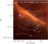 |
Fig. 4 Integrated [C ii] contours over-laid on the false-color IRAC map of the Orion Bar (red: 8.0 μm: 0–3000 MJy/sr, green: 5.8 μm: 0−7000 MJy/sr, blue: 3.6 μm: 0–10 000 MJy/sr). [C ii] is mapped in a strip perpendicular to the Orion Bar. Intensities are labeled in units of K km s-1. The colors in the IRAC map are provided by the signal in the 3.6, 5.8, and 8 μm channels. The yellow circle indicates the HIFI beam size. |
4.1. Orion Bar
4.1.1. [CII]
[C ii] was mapped along a strip perpendicular to the direction of the Bar. Figure 4 shows an overlay of the integrated line intensity on the IRAC 8 μm image. [C ii] shows a very smooth structure, without any indication for clumpiness as seen e.g. in the CO isotopologues, HCN, HCO+, CS and H2CO by Hogerheijde et al. (1995) and Lis & Schilke (2003) and to a lower degree also in the C91α carbon radio recombination line by Wyrowski et al. (1997). This indicates that [C ii] traces mainly the widely distributed, relatively uniform interclump medium. The position, structure, and overall extent of the [C ii] emission in the Orion Bar are similar to the C91α radio recombination line map, which shows, however, a higher contrast and some clumpy substructure close to the emission peak. To some degree that may be due to the insufficient short-spacings of the interferometer data, but it probably also reflects real differences in the excitation. As the C91α emission is much more sensitive to the gas density and temperature than [C ii] (see e.g. Natta et al. 1994), the ratio of the two lines may provide a way to better characterize the transition between the widely distributed gas and the embedded clumps. The [C ii] emission peaks approximately 10′′ deeper into the cloud compared to the PAH emission traced by the IRAC 8 μm map. This coincides approximately with the peak of the H2 1−0 S(1) line observed by Walmsley et al. (2000) and correlates very well with the C2H emission (van der Wiel et al. 2009). A detailed comparison of the stratification in the different tracers will be the topic of a forthcoming paper (Makai et al., in prep.).
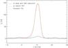 |
Fig. 5 [C ii] profile toward the peak of the Orion Bar emission (5h35m20.6s, −5°25′5′′) averaged over a 43′′ (FWHM) Gaussian beam representing the resolution of the previous KAO observations (solid line). The dotted spectrum represents the widely distributed emission as measured on our secondary OFF position 12.3′ away from the Orion Bar in a region without molecular emission. The dashed lines show Gaussian fits to the two profiles. |
We can compare our data with previous KAO observations of [C ii] in Orion. Boreiko et al. (1988) and Boreiko & Betz (1996) obtained frequency-resolved spectra toward Θ1C, but not toward the Orion Bar. The spectrally unresolved maps of Stacey et al. (1993) and Herrmann et al. (1997) showed approximately the same integrated intensity at the peak of the Orion Bar and toward Θ1C. The Θ1C value from Boreiko & Betz (1996) of 3.8 × 10⁻³ erg cm-2 s-1 sr-1 is, however, 16% lower than the 4.5 × 10⁻³ erg cm-2 s-1 sr-1 derived for the integrated [C ii] intensity at the Orion Bar by Herrmann et al. (1997) scaling all intensities to match the previous value from Stacey et al. (1993) toward Orion KL. Figure 5 shows our [C ii] HIFI profile toward the peak in the Orion Bar after convolution to the 43′′ resolution of the KAO. The integrated intensity of 585 K km s-1 = 4.1 × 10⁻³ erg cm-2 s-1 sr-1 falls between the two quoted KAO values. The discrepancy with the lower value from Boreiko & Betz (1996) can be partially explained by self-chopping of the KAO observations in the very extended emission. Our observation of the secondary OFF position (also shown in Fig. 5) gives an estimate for this extended emission providing a 6% correction of the KAO values. The 9% discrepancy with the Herrmann et al. (1997) value could be due to the uncertainty in the error beam pickup discussed above or the scaling method used in their paper.
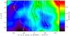 |
Fig. 6 Contours of the [C ii] line peak intensity overlaid on the line width (FWHM) obtained from a Gaussian fit to the [C ii] lines at all points in the Orion Bar map. |
As we find almost perfect Gaussian profiles for the lines in the Orion Bar (see Fig. 5) we performed Gaussian fits to all [C ii] spectra. Figure 6 shows the resulting maps of the fitted amplitude and line width. As the observations by Boreiko & Betz (1996) indicated partially optically thick lines, we expect that the lines become broader toward the peak of the emission due to optical depth broadening. The map, however, does not show any significant change of the line width across the Orion Bar. The FWHM of the line falls between 4.0 and 4.5 km s-1 only becoming broader for the more diffuse emission in the north. Consequently, the amplitude map gives a perfect match to the integrated line map in Fig. 4. As we confirm the significant optical depth in the following section, this indicates that the [C ii] line must be composed of many velocity components which are individually optically thick, instead of a continuous microturbulent medium that only turns optically thick toward the highest column density regions. The corresponding map of the line center velocity only shows a small gradient along the Bar with velocities of about 11 km s-1 in the north-east and 10.5 km s-1 in the south-west.
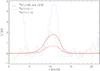 |
Fig. 7 Average profile of the two strongest [13C ii] hyper-fine components in the Orion Bar compared to the [C ii] profile scaled by factors of 0.625/67 and 0.25/67. The profiles were averaged over all pixels with a [C ii] integrated intensity above 700 K km s-1. |
4.1.2. [13CII]
Due to the narrow line width in the Orion Bar, we are able to detect the F = 2−1 and F = 1−0 lines of [13C ii] without noticeable blending with the [C ii] line. Figure 7 shows the line profiles of the two [13C ii] components averaged over the region with the brightest emission, i.e. with [C ii] intensities, above 700 K km s-1. For a comparison, we show the corresponding [C ii] spectra, scaled by factor of 0.625/67 and 0.25/67, respectively. This scaling corresponds approximately to the line intensity of the two [13C ii] transitions expected assuming the canonical abundance ratio and optically thin emission.
 |
Fig. 8 Contours of the [C ii] line center optical depth, derived from the [C ii]/[13C ii] ratio, overlaid on the integrated [C ii] intensities observed toward the Orion Bar. |
When considering the line amplitudes, we find that both hyperfine transitions are approximately 2.5 times brighter than expected for optically thin [C ii] emission and the normal isotopic ratio. Assuming the canonical abundance ratio, this corresponds to a line-center optical depth, of 2.2. The good signal to noise ratio of the data allows us to perform Gaussian fits to the hyperfine lines over the full map, providing the intensity ratio map. Using Eq. (5) and assuming no chemical fractionation, we can translate this into the optical depth map. Figure 8 shows the resulting line center optical depth, , overlaid on the integrated [C ii] intensitiy map. Here, we have added both hyperfine transitions to increase the signal to noise. No reliable values can be derived for τ ≲ 0.8 as Eq. (5) turns very flat for low optical depths. Hence, the corresponding points have been masked-out. We find a good correlation of the optical depth structure with the intensity map. The map confirms that the area of bright [C ii] emission has optical depths above two and the peak optical depth of 3.4 occurs close to the intensity peak, but we also see a small general shift of the optical depth structure relative to the intensity structure away from the exciting Trapezium cluster. This is consistent with the picture of hotter gas at the PDR front and somewhat cooler, but a higher column density gas deeper into the cloud.
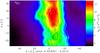 |
Fig. 9 Contours of the [C ii] excitation temperature overlaid on the derived column densities toward the Orion Bar. |
To better quantify this, we use Eq. (3) to compute the excitation temperatures, and Eq. (2) together with the optical depth correction in Eq. (5) to compute the total C+ column density. The resulting distribution is shown in Fig. 96. In the range of significant optical depths, the excitation temperatures fall between 190 and 265 K. For τ ≤ 0.8 we assumed a constant excitation temperature of 190 K and directly used the optically thin approximation of Eq. (2) to compute the C+ column density.
Our excitation temperatures are in agreement with the average value of 220 K and 215 K derived by Herrmann et al. (1997) and Sorochenko & Tsivilev (2000), respectively, for the Orion Bar. Interclump gas at this temperature with a density around 105 cm-3 also explains the C91α observations of Wyrowski et al. (1997). However, Natta et al. (1994) and Walmsley et al. (2000) obtain much higher temperatures from observations of the radio recombination lines. This could indicate nonthermal emission, dielectronic recombination, or simply different gas components contributing to the [C ii] and C91α emission (Natta et al. 1994; Sorochenko & Tsivilev 2000).
At the KAO resolution, our approach provides a column density of 7−8 × 1018 cm-2, more than two times higher than the value of Herrmann et al. (1997), consistent with our [C ii] optical depth exceeding the value derived by Boreiko & Betz (1996) by about the same factor. The discrepancy can be explained to a large degree by the use of the line-averaged optical depth in Herrmann et al. (1997), underestimating the peak optical depth by a factor 0.64 for a Gaussian velocity distribution (see Sect. 2.3), and the use of different spectroscopic parameters, as discussed in Sect. 3.1. Our peak C+ column density of 13 × 1018 cm-2 implies a configuration where most of the line-of-sight column density of the Orion Bar of NH ≈ 13 × 1022 cm-2 (e.g. Hogerheijde et al. 1995) forms a PDR with complete ionization of the gas-phase carbon – abundance X(C) = n(C)/(n(H) + 2n(H2)) = 1.2 × 10⁻⁴ for dense clouds (Wakelam & Herbst 2008). A surprising result is, however, the relatively high C+ column density in front and behind the Bar. Molecular line observations (e.g. Hogerheijde et al. 1995; van der Werf et al. 1996) deduced column densities that are a factor ten lower than in the Bar. Consequently, at least half of the [C ii] emission in the veil must stem from atomic, diffuse material.
Figure 9 also shows a 5−8′′ relative shift between the column density and the excitation temperature distributions, with the higher temperatures toward the illuminating source. The new observations thus resolve a temperature gradient in C+, consistent with the overall stratified structure of the Orion Bar PDR. The resulting intensity profile then represents a convolution of the density and temperature structures.
4.1.3. Line averages
To verify the effect of the assumption of the Gaussian velocity distribution, we repeated the analysis for selected subregions considering the line-averaged [C ii]/[13C ii] intensity ratio, i.e. ⟨ τ ⟩ instead of . This is also the only possible analysis for the other sources, where the signal-to-noise ratio is lower and the line profiles are highly structured, so that the assumption of a Gaussian velocity distribution is clearly incorrect. The use of the line-averaged optical depth, ⟨ τ ⟩ , corresponds to the assumption of a macro-turbulent situation, where [C ii] turns independently optically thick in all velocity channels, while the method assumes a microturbulent Gaussian velocity distribution for all tracers, where [C ii] turns optically thick only at the line center. A preference for one of the methods is only possible based on detailed knowlegde of the source structure. The ⟨ τ ⟩ results for all sources are included in the last two columns in Table 2.
For the Orion Bar, the ⟨ τ ⟩ results always fall below the column densities from the line-center optical depth, by 30−35% in spite of the almost Gaussian line profiles. A possible explanation is the systematic difference in the line width between the [13C ii] and the [C ii] lines, beyond the expected optical-depth broadening. As seen in the average spectrum shown in Fig. 7, but also in the map of [13C ii] line widths in Fig. 6, the [13C ii] lines are always 1.0−1.5 km s-1 narrower than the [C ii] lines. As a consequence, the intensity ratio is even larger than the standard elemental isotopic ratio in the line wings (well visible in the blue wing in Fig. 7). Together with the constant [C ii] line width discussed in the previous section, the enhanced intensity ratio in the wings indicates different velocity distributions for C+ and 13C+. Consequently, neither the method nor the ⟨ τ ⟩ method provides accurate results. The 30−35% of the emission remaining in the wings of the [C ii] line when fitting it with the profile of the [13C ii] lines provide an estimate for the accuracy of our analysis.
The ⟨ τ ⟩ values from the average spectra in Table 2 also confirm the spatial gradient in the column densities seen in Fig. 9. This can be seen through analyzing the bright gas in front and behind the Orion Bar. To explore this issue we selected all pixels with a [C ii] intensity between 450 and 650 K km s-1 north-west, i.e. in the direction of the illuminating Trapezium stars, and south-east of the Bar. We find significantly higher optical depths behind the Bar, while the gas in front of the Bar is typically hotter by about 20 K, but thinner by a factor 1.7.
None of the average spectra show an indication for an enhanced C+/13C+ fractionation ratio. This also applies to the spectra from the veil in front and behind the Bar, where we were not able to detect a significant deviation from the elemental abundance ratio due to the relatively larger baseline uncertainties at lower intensities of the [13C ii] lines. Our [13C ii] observations are consistent with negligible carbon fractionation and an enhanced optical depth of the main isotopic line for high column densities. This is in agreement with a previous detection of the [13C i] F = 5/2−3/2 transition by Keene et al. (1998) in a selected clump, where the observed 13C/C ratio showed no fractionation effect, in contrast to the complementary observations for 13C18O and C18O.
An indication for an enhanced fractionation ratio is, however, seen in the velocity structure when considering the wings of the bright line profiles. The broader [C ii] lines, showing enhanced [C ii]/[13C ii] intensity ratio in the wings (e.g. in Fig. 7), indicate that an additional gas component, with broader velocity dispersion and enhanced fractionation ratio, thus invisible in [13C ii], contributes to the [C ii] profiles. The constancy of the [C ii] line width then can be explained by the mutual compensation of the relatively larger contribution from the low-velocity dispersion Orion Bar material with the optical depth broadening there. To sustain the enhanced intensity ratio, the broad velocity gas component should have moderate gas densities of 103−104 cm-3 and face moderate UV fields (χ ≈ 103, see Sect. 2).
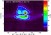 |
Fig. 10 Position-velocity diagram of the [C ii] line for the measured cut through the Mon R2 PDR. |
4.2. Mon R2
4.2.1. [CII]
The [C ii] OTF map of Mon R2 consists of a single strip across the ultracompact H ii region from north-east to south-west (see Fuente et al. 2010). Figure 10 shows the position-velocity diagram for that cut. This is important for understanding the origin of the components in the spectral profile, in comparison with the [13C ii] lines. We find a ring-like structure in the position-velocity space, with two well separated components toward the center of the H ii region. A better understanding of the position velocity structure can be obtained by combining this information with equivalent maps in several other tracers (Pilleri et al. 2012a). In particular the comparison with water lines, that show up in absorption in the blue component but in emission in the red component, suggests that the diagram traces a PDR around the H ii region that is accelerated by the radiative pressure from the central source, so that the back side is red-shifted and the front side blue-shifted relative to the systemic velocity of the source. However, observations show some asymmetry between the expanding and receding layer and part of the central dip could also stem from self-absorption in the optically thick line.
4.2.2. [13CII]
The dual-beam-switch observations of the [13C ii] lines were performed at the center position of the OTF strip (position 0 in Fig. 10), i.e. not at the peak of the [C ii] emission. Future follow-up observations at the peak position will provide a better accuracy.
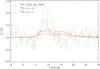 |
Fig. 11 Comparison of the profiles of the [13C ii] hyperfine lines in Mon R2 with the [C ii] profile in the same spectrum scaled by the factors 0.25/67 and 0.125/67. The [13C ii] F = 2−1 component is blended with the main isotopic line so that is not shown here. |
Figure 11 shows the line profiles of the [13C ii] components compared to the corresponding [C ii] spectrum, scaled by the factor 0.25/67 and 0.125/67 indicating the expected strength of the F = 1−0 and F = 1−1 hyperfine components in case of optically thin emission and a canonical abundance ratio (see Sect. 3.1). Due to the large width of the [C ii] line, the F = 2−1 component falls in the wing of the [C ii] emission and we cannot estimate its strength. The striking result for the other two components is the large difference in their spectral shape compared to the main isotopic line. The two hyperfine components show the same line shape, peaking at about 9 km s-1 and have an intensity ratio of about a factor two. The peak agrees with a flat-top emission part of the [C ii] line that would be characteristic for optically thick emission and is about three times brighter than the scaled blue [C ii] component. This is not reflected in the average optical depth ⟨ τ ⟩ derived from the integrated line in Table 2 due to the large differences in the line shapes. To get an estimate for the two main velocity components, we have split the integration interval at 12.5 km s-1 and include the corresponding results in Table 2. This increases the relative uncertainties, but allows deriving independent quantitative results for the components that show a very different behavior. For the blue-shifted foreground component, we find the highest [C ii] optical depth in our sample.
A big surprise is the complete absence of redshifted emission from the back of the H ii region in [13C ii]. The red-shifted [C ii] line has approximately the same brightness as the blue-shifted component, but any possible [13C ii] emission must be weaker than expected from optically thin emission and normal abundance ratios. For both hyperfine components, emission at the 0.1 K level can be excluded in spite of the baseline uncertainties. This provides a direct observation of fractionation in a PDR, resulting in an enhanced 12C+/13C+ ratio. However, when considering the extreme uncertainties in Table 2, stemming from all possible baseline subtractions and the possibility that the redshifted [C ii] line may be optically thin, while the blueshifted line has an optical depth >3, the error bars for the 12C+/13C+ fractionation ratio still include the standard elemental isotopic ratio so that even this case is not unambiguous.
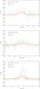 |
Fig. 12 Comparison of the profiles of the [13C ii] hyperfine lines in NGC 3603 MM2 (upper panel), the Carina North PDR (central panel), and NGC 7023 North (lower panel) with the [C ii] profiles from the same positions scaled by the factors corresponding to optically thin emission and the standard abundance ratio for the resolved hyperfine components. For NGC 3603 MM2 and Carina North, the [13C ii] F = 2−1 component falls into a self-chopping feature of the main isotopic line so that is not shown here. |
4.3. NGC 3603, Carina, and NGC 7023
Figure 12 shows the spectra for NGC 3603, Carina North, and NGC 7023, obtained in the same way as Fig.11 for Mon R2. As discussed in Sect. 3.2, in NGC 3603 and Carina the F = 2−1 component falls into a [C ii] spectral feature resulting from self-chopping in the observation and it cannot be resolved. However, the two weaker components are resolved. There is no indication for a spectral difference with respect to the [C ii] line and the corresponding line ratio agrees with the expected value from Sect. 3.1. In both sources, the [13C ii] lines are about 2.5 times stronger than expected for optically thin [C ii] emission and the normal abundance ratio. This indicates an optical depth in the main isotopic line of 2.2−2.4.
The equivalent observation of the Carina South PDR, provided no detections of [13C ii]. At the frequency of the F = 2−1 transition we find a weak emission component, but we rather attribute this to a separate [C ii] velocity component in the complex velocity profile. As the [C ii] line brightness is more than three times weaker than in the other sources, the non-detection is consistent with the expected line strength in the optically thin case, or for moderate [13C ii] line enhancements as seen in the other sources.
The narrow [C ii] line in NGC 7023 is well separated from the [13C ii] F = 2−1 component, so that this is the only case where we spectrally resolve all three hyperfine components. Moreover, the narrow lines provide a very small uncertainty for the line intensity from the baseline subtraction, leading to accurate relative intensities. The average optical depth enhancement of the [13C ii] lines is moderate, but we also find a significantly different behavior for different velocity components seen in the [C ii] line profiles. The [13C ii] lines mainly trace the component at 2.8 km s-1, corresponding to the molecular material in the PDR (see e.g. Gerin et al. 1998). Here, we find a significant optical depth of the [C ii] line as indicated by a decreased [C ii]/[13C ii] intensity ratio. The component at 4 km s-1 was identified as separate filament (Fuente et al. 1996), associated with the ionized material in the cavity (Joblin et al. 2010). It is also seen in [13C ii] and shows an intensity ratio corresponding to the elemental isotopic ratio. Finally there is a high velocity wing, with velocities around 0 km s-1. This component appears to show an increased 12C+/13C+ fractionation ratio with [13C ii] intensities below the scaled [C ii] intensity for all three hyperfine components. However, our signal-to-noise ratio is insufficient to draw definite conclusions obout the [C ii]/[13C ii] intensity ratio in that wing. Due to the almost Gaussian velocity components, the estimate of the C+ column density from the integrated line parameters should be a reasonable average, slightly underestimating the optical depth from the PDR and slightly overestimating the contribution from the ionized gas in the cavity. For a total column density NH ≈ 1.3 × 1022 cm-2 at the position of our observation (Joblin et al. 2010) this indicates that more than half of the carbon in the gas phase is in the form of C+.
5. Discussion
The detection of carbon fractionation in dense clouds remains challenging. For the two species involved in the most important carbon fractionation reaction, C+ and CO, the lines of the main isotopologue are often optically thick, with a considerable uncertainty in the optical depth. Consequently, it is difficult to determine accurate column densities and the corresponding CO/13CO or C C+ ratios. Our observations and simulations have confirm this for the CC+ ratio. Observations of 13C18O are a possible way forward, but challenging due to the low line intensities and biased toward high column densities. In addition, they cannot trace the impact of isotope-selective photodissociation due to the self-shielding of the main isotopologue.
Our model predictions for PDRs indicate that the observed fractionation ratio in all tracers is dominated by the chemical fractionation reaction (C 1), while isotopic-selective photo-dissociation plays a minor role. The chemical fractionation increases the CC+ ratio relative to the elemental isotopic ratio in the gas. In terms of the observable [C ii]/[13C ii] line intesnity ratio, this could lead to an increase by a factor of a few under most favorable conditions. These correspond to inner layers of moderate density, moderate UV PDRs, or dense gas exposed to low UV fields, such as clumps in an inhomogeneous PDR, embedded in and partially shielded by a thinner interclump medium. The main requirement for an observable increase of the [C ii]/[13C ii] ratio is, however, that the geometry and velocity distribution prevent a high [C ii] optical depth. Unfortunately, in most geometries, the conditions providing an increased isotopic ratio also result in high optical depths of the [C ii] line that reduces the observed [C ii]/[13C ii] intensity ratio below the canonical value.
Our observations show that most of the [C ii] emission must stem from a widely distributed, low-density component in PDRs, being more smoothly distributed than many high-density tracers. Only in Mon R2, where the H ii region is still expanding into the surrounding high-density core, a relatively homogeneous high-density PDR is formed. The observational results on the [C ii]/[13C ii] intensity ratio roughly follow model predictions in Sect. 2, without providing enough statistics for a qualitative confirmation. For most of the PDRs, the average [C ii]/[13C ii] intensity ratio is reduced compared to the isotopic ratio due to the optical thickness of the [C ii] line. Details strongly depend on the exact geometry. Assuming the standard elemental ratio for the CC+ abundance ratio, we can determine the optical depth and consequently the C+ column density from the intensity ratio. The optical depth of the main isotopic line varies considerably across the line profile and between the different PDRs, with peak values above three in the Orion Bar and Mon R2.
Indications for an increased [C ii]/[13C ii] intensity ratio are found when studying detailed line profiles, allowing to distinguish different velocity components in the telescope beam. In three cases, we find components showing evidence of C+ fractionation. Unfortunately, none of them allows to unambiguously quantify the degree of fractionation due to the large error bars dominated by baseline uncertainties (see Table 2). The clearest case is the non-detection of [13C ii] emission in the red-shifted component in Mon R2. If we interpret the red component as the receding inner back side of the expanding H ii region, it represents a dense, face-on PDR layer which should be at least partially optically thick in [C ii]. As the front side shows the same integrated [C ii] intensity, but no fractionation and a very high [C ii] optical depth, the actual configuration must be asymmetric. The situation if even more puzzling, as our models predict negligible fractionation for this high-UV field PDR. Further high-resolution observations are required to understand why the red-shifted material differs from the material in the front of the H ii region. The second case is provided by the wings of the line profiles in the Orion Bar, probably associated with diffuse gas with a broader velocity distribution, which may represent extended, possibly diffuse H ii gas in the Orion veil. To confirm this origin, deeper integrations at positions away from the Orion Bar are needed. A final case may be given by the blue-wing material seen in NGC 7023. However, in all three cases the step from a pure detection of fractionation to a full quantitative assessment requires observations with a somewhat better signal-to-noise ratio than obtained here.
All other fractionation reactions for 13C have lower excess energies and are, therefore, relevant only in cold gas.
1011K km s-1 = 7.11 × 10⁻³ erg s-1 cm-2 sr-1 at the frequency of the [C ii] transition.
The general expression, also covering the high optical depth limit, is given e.g. by Phillips et al. (1979).
We do not include a separate interclump medium, but rather represent interclump material by the equivalent mass of an ensemble of small, transient, low-density clumps.
Our line ratios differ from those given by Cooksy et al. (1986) and used in previous astronomical studies (0.444:0.356:0.20). This discrepancy may account for the anomaly reported recently by Graf et al. (2012), who observed a F = 2−1: F = 1−0 ratio in NGC 2024 that was considerably higher than that predicted by Cooksy et al. (1986). It also implies a minor revision to the elemental isotopic ratio inferred by Boreiko & Betz (1996) from observations of the F = 2−1 and 1−0 transitions observed toward M42. That study applied a correction factor to account for the F = 1−1 transition, which was not covered by the available instrumental bandwidth. With our revised line strengths, the correction factor decreases from 5/4 to 8/7, resulting in a 9.4% increase in the inferred elemental ratio, from the range of 52−61 given by Boreiko & Betz (1996) to 57−67. This, in turn, resolves the small discrepancy, noted by Boreiko & Betz (1996), between the isotopic ratio obtained from observations of [13C ii] and the value of 67 ± 3 inferred from observations of 13CO.
When scaling the measured intensities to the main beam efficiency, i.e. assuming less extended emission, the optical depth does not change, but the excitation temperature and C+ column densities increase by 30% relative to the values given here.
Acknowledgments
This work was supported by the Deutsche Forschungsgemeinschaft, DFG project number Os 177/1–1 and SFB 956 C1. Additional support for this paper was provided by NASA through an award issued by JPL/Caltech and by Spanish program CONSOLIDER INGENIO 2010, under grant CSD2009-00038 Molecular Astrophysics: The Herschel and ALMA Era (ASTROMOL). We thank Paul Goldsmith and an anonymous referee for many helpful comments. HIFI has been designed and built by a consortium of institutes and university departments from across Europe, Canada and the US under the leadership of SRON Netherlands Institute for Space Research, Groningen, The Netherlands with major contributions from Germany, France and the US. Consortium members are: Canada: CSA, U.Waterloo; France: CESR, LAB, LERMA, IRAM; Germany: KOSMA, MPIfR, MPS; Ireland, NUI Maynooth; Italy: ASI, IFSI-INAF, Arcetri-INAF; Netherlands: SRON, TUD; Poland: CAMK, CBK; Spain: Observatorio Astronómico Nacional (IGN), Centro de Astrobiología (CSIC-INTA); Sweden: Chalmers University of Technology – MC2, RSS & GARD, Onsala Space Observatory, Swedish National Space Board, Stockholm University – Stockholm Observatory; Switzerland: ETH Zürich, FHNW; USA: Caltech, JPL, NHSC.
References
- Bergin, E. A., & Herschel Hexos Team 2011, in IAU Symp., 280, 93 [Google Scholar]
- Boreiko, R. T., & Betz, A. L. 1996, ApJ, 467, L113 [NASA ADS] [CrossRef] [Google Scholar]
- Boreiko, R. T., Betz, A. L., & Zmuidzinas, J. 1988, ApJ, 325, L47 [NASA ADS] [CrossRef] [PubMed] [Google Scholar]
- Burgh, E. B., France, K., & McCandliss, S. R. 2007, ApJ, 658, 446 [NASA ADS] [CrossRef] [Google Scholar]
- Cooksy, A. L., Blake, G. A., & Saykally, R. J. 1986, ApJ, 305, L89 [NASA ADS] [CrossRef] [Google Scholar]
- de Graauw, T., Helmich, F. P., Phillips, T. G., et al. 2010, A&A, 518, L6 [NASA ADS] [CrossRef] [EDP Sciences] [Google Scholar]
- Draine, B. T. 1978, ApJS, 36, 595 [NASA ADS] [CrossRef] [Google Scholar]
- Flannery, B. P., Roberge, W., & Rybicki, G. B. 1980, ApJ, 236, 598 [NASA ADS] [CrossRef] [Google Scholar]
- Flower, D. R., & Launay, J. M. 1977, J. Phys. B Atom. Mol. Phys., 10, 3673 [NASA ADS] [CrossRef] [Google Scholar]
- Fuente, A., Martin-Pintado, J., Neri, R., Rogers, C., & Moriarty-Schieven, G. 1996, A&A, 310, 286 [NASA ADS] [Google Scholar]
- Fuente, A., Berné, O., Cernicharo, J., et al. 2010, A&A, 521, L23 [NASA ADS] [CrossRef] [EDP Sciences] [Google Scholar]
- Garstang, R. H. 1995, ApJ, 447, 962 [NASA ADS] [CrossRef] [Google Scholar]
- Gerin, M., Phillips, T. G., Keene, J., Betz, A. L., & Boreiko, R. T. 1998, ApJ, 500, 329 [NASA ADS] [CrossRef] [Google Scholar]
- Ginard, D., González-García, M., Fuente, A., et al. 2012, A&A, 543, A27 [NASA ADS] [CrossRef] [EDP Sciences] [Google Scholar]
- Graf, U. U., Simon, R., Stutzki, J., et al. 2012, A&A, 542, L16 [NASA ADS] [CrossRef] [EDP Sciences] [Google Scholar]
- Herrmann, F., Madden, S. C., Nikola, T., et al. 1997, ApJ, 481, 343 [NASA ADS] [CrossRef] [Google Scholar]
- Hogerheijde, M. R., Jansen, D. J., & van Dishoeck, E. F. 1995, A&A, 294, 792 [NASA ADS] [Google Scholar]
- Joblin, C., Pilleri, P., Montillaud, J., et al. 2010, A&A, 521, L25 [NASA ADS] [CrossRef] [EDP Sciences] [Google Scholar]
- Keene, J., Schilke, P., Kooi, J., et al. 1998, ApJ, 494, L107 [NASA ADS] [CrossRef] [Google Scholar]
- Langer, W. D., & Penzias, A. A. 1990, ApJ, 357, 477 [NASA ADS] [CrossRef] [Google Scholar]
- Langer, W. D., & Penzias, A. A. 1993, ApJ, 408, 539 [NASA ADS] [CrossRef] [Google Scholar]
- Langer, W. D., Graedel, T. E., Frerking, M. A., & Armentrout, P. B. 1984, ApJ, 277, 581 [NASA ADS] [CrossRef] [Google Scholar]
- Launay, J.-M., & Roueff, E. 1977, J. Phys. B Atom. Mol. Phys., 10, 879 [Google Scholar]
- Lis, D. C., & Schilke, P. 2003, ApJ, 597, L145 [NASA ADS] [CrossRef] [Google Scholar]
- Liszt, H. S. 2007, A&A, 476, 291 [NASA ADS] [CrossRef] [EDP Sciences] [Google Scholar]
- Menten, K. M., Reid, M. J., Forbrich, J., & Brunthaler, A. 2007, A&A, 474, 515 [NASA ADS] [CrossRef] [EDP Sciences] [Google Scholar]
- Mookerjea, B., Ghosh, S. K., Kaneda, H., et al. 2003, A&A, 404, 569 [NASA ADS] [CrossRef] [EDP Sciences] [Google Scholar]
- Natta, A., Walmsley, C. M., & Tielens, A. G. G. M. 1994, ApJ, 428, 209 [NASA ADS] [CrossRef] [Google Scholar]
- Okada, Y., Pilleri, P., Berné, O., et al. 2013, A&A, submitted [Google Scholar]
- Ossenkopf, V., Röllig, M., Kramer, C., et al. 2011, in EAS Publ. Ser., 52, eds. M. Röllig, R. Simon, V. Ossenkopf, & J. Stutzki, 181 [Google Scholar]
- Ott, S. 2010, in Astronomical Data Analysis Software and Systems XIX, eds. Y. Mizumoto, K.-I. Morita, & M. Ohishi, ASP Conf. Ser., 434, 139 [Google Scholar]
- Phillips, T. G., Huggins, P. J., Wannier, P. G., & Scoville, N. Z. 1979, ApJ, 231, 720 [NASA ADS] [CrossRef] [Google Scholar]
- Pilbratt, G. L., Riedinger, J. R., Passvogel, T., et al. 2010, A&A, 518, L1 [CrossRef] [EDP Sciences] [Google Scholar]
- Pilleri, P., Fuente, A., Cernicharo, J., et al. 2012a, A&A, 544, A110 [NASA ADS] [CrossRef] [EDP Sciences] [Google Scholar]
- Pilleri, P., Montillaud, J., Berné, O., & Joblin, C. 2012b, A&A, 542, A69 [NASA ADS] [CrossRef] [EDP Sciences] [Google Scholar]
- Roelfsema, P. R., Helmich, F. P., Teyssier, D., et al. 2012, A&A, 537, A17 [NASA ADS] [CrossRef] [EDP Sciences] [Google Scholar]
- Röllig, M., & Ossenkopf, V. 2013, A&A, 550, A56 (Paper I) [NASA ADS] [CrossRef] [EDP Sciences] [Google Scholar]
- Röllig, M., Abel, N. P., Bell, T., et al. 2007, A&A, 467, 187 [NASA ADS] [CrossRef] [EDP Sciences] [Google Scholar]
- Röllig, M., Kramer, C., Rajbahak, C., et al. 2011, A&A, 525, A8 [Google Scholar]
- Sakai, N., Saruwatari, O., Sakai, T., Takano, S., & Yamamoto, S. 2010, A&A, 512, A31 [NASA ADS] [CrossRef] [EDP Sciences] [Google Scholar]
- Schaefer, H. F., & Klemm, R. A. 1970, Phys. Rev. A, 1, 1063 [NASA ADS] [CrossRef] [Google Scholar]
- Sheffer, Y., Rogers, M., Federman, S. R., Lambert, D. L., & Gredel, R. 2007, ApJ, 667, 1002 [NASA ADS] [CrossRef] [Google Scholar]
- Simon, R., Stutzki, J., Sternberg, A., & Winnewisser, G. 1997, A&A, 327, L9 [NASA ADS] [Google Scholar]
- Smith, N. 2006, MNRAS, 367, 763 [NASA ADS] [CrossRef] [Google Scholar]
- Sonnentrucker, P., Welty, D. E., Thorburn, J. A., & York, D. G. 2007, ApJS, 168, 58 [NASA ADS] [CrossRef] [Google Scholar]
- Sorochenko, R. L., & Tsivilev, A. P. 2000, Astron. Rep., 44, 426 [NASA ADS] [CrossRef] [Google Scholar]
- Stacey, G. J., Jaffe, D. T., Geis, N., et al. 1993, ApJ, 404, 219 [CrossRef] [Google Scholar]
- Stolte, A., Brandner, W., Brandl, B., & Zinnecker, H. 2006, AJ, 132, 253 [NASA ADS] [CrossRef] [Google Scholar]
- Stutzki, J., Bensch, F., Heithausen, A., Ossenkopf, V., & Zielinsky, M. 1998, A&A, 336, 697 [NASA ADS] [Google Scholar]
- van den Ancker, M. E., The, P. S., Tjin A Djie, H. R. E., et al. 1997, A&A, 324, L33 [NASA ADS] [Google Scholar]
- van der Werf, P. P., Stutzki, J., Sternberg, A., & Krabbe, A. 1996, A&A, 313, 633 [NASA ADS] [Google Scholar]
- van der Wiel, M. H. D., van der Tak, F. F. S., Ossenkopf, V., et al. 2009, A&A, 498, 161 [NASA ADS] [CrossRef] [EDP Sciences] [Google Scholar]
- Visser, R., van Dishoeck, E. F., & Black, J. H. 2009, A&A, 503, 323 [NASA ADS] [CrossRef] [EDP Sciences] [Google Scholar]
- Wakelam, V., & Herbst, E. 2008, ApJ, 680, 371 [NASA ADS] [CrossRef] [Google Scholar]
- Walmsley, C. M., Natta, A., Oliva, E., & Testi, L. 2000, A&A, 364, 301 [NASA ADS] [Google Scholar]
- Wiese, W., & Fuhr, J. 2007, J. Phys. Chem. Ref. Data, 36, 1287 [CrossRef] [Google Scholar]
- Wilson, T. L. 1999, Rep. Prog. Phys., 62, 143 [Google Scholar]
- Wilson, N. J., & Bell, K. L. 2002, MNRAS, 337, 1027 [NASA ADS] [CrossRef] [Google Scholar]
- Wyrowski, F., Schilke, P., Hofner, P., & Walmsley, C. M. 1997, ApJ, 487, L171 [NASA ADS] [CrossRef] [Google Scholar]
- Xu, Y., Shen, Z.-Q., Yang, J., et al. 2006, AJ, 132, 20 [NASA ADS] [CrossRef] [Google Scholar]
All Tables
Summary of integrated line intensities from the observations and derived parameters.
All Figures
|
Fig. 1 Top: abundance distribution of C+ and CO and the corresponding 13C isotopologues for a model with nsurf = 104 cm-3, 1000 χ0 and 1000 M⊙. The blue curve shows the corresponding gas temperature structure determining the emissivity. Bottom: resulting integrated optically thin line emissivity ∫ϵdv in K km s-1/(cm-3 pc) for the [C ii] and [13C ii] lines (black curves) as a function of the clump radius. The red line shows the intensity ratio provided by the two curves. |
| In the text | |
|
Fig. 2 Differences between [C ii] emissivity and [13C ii] emissivity multiplied by the standard elemental isotopic ratio of 67 showing conditions where a increased C+/13C+ fractionation ratio turns into an observable increased [C ii]/[13C ii] intensity ratio. The upper plot uses a radiation field of 1000χ0 and varies the surface gas density: 103 cm-3 (black), 104 cm-3 (grey), 105 cm-3 (blue), 106 cm-3 (red). The lower plot uses a gas density of nsurf = 104 cm-3 and varies the radiation field: 1χ0 (black), 10χ0 (grey), 100χ0 (blue), 103χ0 (cyan), 104χ0 (green), 105χ0 (red), 106χ0 (orange). The dashed line at 10 K km s-1 (cm-3 pc)-1 gives a rough indication what differences might be observable with current technology in a deep integration. |
| In the text | |
|
Fig. 3 Clump integrated intensity ratio ∫I([C ii])dv/∫I([13C ii])dv vs. [C ii] intensity from the KOSMA-τ model for different parameters. The model parameters n, M, and χ, are coded as size, shape, and color of the respective symbols. The red horizontal line denotes the assumed elemental abundance ratio [12C]/[13C] of 67. The insert demonstrates the underlying column density ratio for the different clumps. For [13C ii], we sum over all hyperfine components. |
| In the text | |
|
Fig. 4 Integrated [C ii] contours over-laid on the false-color IRAC map of the Orion Bar (red: 8.0 μm: 0–3000 MJy/sr, green: 5.8 μm: 0−7000 MJy/sr, blue: 3.6 μm: 0–10 000 MJy/sr). [C ii] is mapped in a strip perpendicular to the Orion Bar. Intensities are labeled in units of K km s-1. The colors in the IRAC map are provided by the signal in the 3.6, 5.8, and 8 μm channels. The yellow circle indicates the HIFI beam size. |
| In the text | |
|
Fig. 5 [C ii] profile toward the peak of the Orion Bar emission (5h35m20.6s, −5°25′5′′) averaged over a 43′′ (FWHM) Gaussian beam representing the resolution of the previous KAO observations (solid line). The dotted spectrum represents the widely distributed emission as measured on our secondary OFF position 12.3′ away from the Orion Bar in a region without molecular emission. The dashed lines show Gaussian fits to the two profiles. |
| In the text | |
|
Fig. 6 Contours of the [C ii] line peak intensity overlaid on the line width (FWHM) obtained from a Gaussian fit to the [C ii] lines at all points in the Orion Bar map. |
| In the text | |
|
Fig. 7 Average profile of the two strongest [13C ii] hyper-fine components in the Orion Bar compared to the [C ii] profile scaled by factors of 0.625/67 and 0.25/67. The profiles were averaged over all pixels with a [C ii] integrated intensity above 700 K km s-1. |
| In the text | |
|
Fig. 8 Contours of the [C ii] line center optical depth, derived from the [C ii]/[13C ii] ratio, overlaid on the integrated [C ii] intensities observed toward the Orion Bar. |
| In the text | |
|
Fig. 9 Contours of the [C ii] excitation temperature overlaid on the derived column densities toward the Orion Bar. |
| In the text | |
|
Fig. 10 Position-velocity diagram of the [C ii] line for the measured cut through the Mon R2 PDR. |
| In the text | |
|
Fig. 11 Comparison of the profiles of the [13C ii] hyperfine lines in Mon R2 with the [C ii] profile in the same spectrum scaled by the factors 0.25/67 and 0.125/67. The [13C ii] F = 2−1 component is blended with the main isotopic line so that is not shown here. |
| In the text | |
|
Fig. 12 Comparison of the profiles of the [13C ii] hyperfine lines in NGC 3603 MM2 (upper panel), the Carina North PDR (central panel), and NGC 7023 North (lower panel) with the [C ii] profiles from the same positions scaled by the factors corresponding to optically thin emission and the standard abundance ratio for the resolved hyperfine components. For NGC 3603 MM2 and Carina North, the [13C ii] F = 2−1 component falls into a self-chopping feature of the main isotopic line so that is not shown here. |
| In the text | |
Current usage metrics show cumulative count of Article Views (full-text article views including HTML views, PDF and ePub downloads, according to the available data) and Abstracts Views on Vision4Press platform.
Data correspond to usage on the plateform after 2015. The current usage metrics is available 48-96 hours after online publication and is updated daily on week days.
Initial download of the metrics may take a while.